Fundamental building blocks of strongly correlated wave functions

Abstract

The calculation of realistic N-body wave functions for identical fermions is still an open problem in physics, chemistry, and materials science, even for N as small as two. A recently discovered fundamental algebraic structure of many-body Hilbert space allows an arbitrary many-fermion wave function to be written in terms of a finite number of antisymmetric functions called shapes. Shapes naturally generalize the single-Slater-determinant form for the ground state to more than one dimension. Their number is exactly $N!^{d-1}$ in $d$ dimensions. An efficient algorithm is described to generate all fermion shapes in spaces of odd dimension, which improves on a recently published general algorithm. The results are placed in the context of contemporary investigations of strongly correlated electrons.

1 Introduction

The study of strong correlations has emerged as the focal point of both fundamental and applied research in physics, chemistry, and materials science. The reason is that modern functional materials fall in between the standard textbook limits of ionic and metallic (or covalent) bonding. In particular the two currently most interesting classes of materials, the high-temperature superconducting cuprates and pnictides, both exhibit a fascinating mixture of ionicity and metallicity Lazic15 ; Borisenko16 which remains to be unravelled. New tools and approaches are constantly being sought Hyowon14 for the description of electrons which inhabit active (open) orbitals in these materials, for which the paradigm “strongly correlated electrons” has been coined long ago.

In cuprates at least, the experimental evidence points to a separation of roles between the electrons occupying copper and oxygen orbitals, such that, roughly speaking, the coppers are responsible for the local, and the oxygens for the extended degrees of freedom Niksic13 . Because of strong Cu–O hybridization, this separation is partly a dynamical phenomenon OSBarisic12 , and partly produces real-space disorder Bianconi87a ; Tahir-Kheli11 ; Campi14 . It leads to a picture of network GBianconi12 or percolation Tahir-Kheli13 conductivity, in which it may be possible to reconcile the local strongly correlated behavior with Fermi-liquid transport properties Mirzaei12 . In particular, if the hole concentration is $1+x$, the transport properties in the superconducting range of dopings scale with $x$, indicating that the “$1$” hole remains localized Mirzaei12 ; Chan14a .

Remarkably, the outlines of a similar situation can be discerned in the case of hydrogen disulphide. It becomes superconducting at high temperature Drozdov15 only after undergoing a structural phase transition Einaga16 at $\sim 150$ GPa, which necessarily involves the active sulphur orbitals. Similarly, a rearrangement of orbital content is inferred for the superconducting wave function Bussmann-Holder16 .

The principal issue in strong correlations is the need to satisfy some dynamical restriction (e.g. no double occupation of a $d$ orbital) simultaneously with the Pauli principle. The problem is that the Pauli principle is kinematically so restrictive that little configuration space remains for the dynamically induced correlations, so one is at a loss to understand how the system manages to satisfy both. Indeed the weak-coupling paradigm is so ubiquitous precisely because the system usually does not manage both, instead it looks almost as the non-interacting one even in the presence of strong interactions: this is the well-known Fermi liquid.

Recently, a new description of fermion many-body states has emerged Sunko16-1 which promises to shed some light on the above issues from a fundamental point of view. It turns out that every system of $N$ identical (i.e. spinless or spin-polarized) fermions in $d$ dimensions has a number of special states called shapes, which are distinguished by a certain type of irreducibility, such that they cannot be interpreted as consisting of lower-energy states, even when their energy is high. Although their number is absolutely very large ($N!^{d-1}$), it is vanishingly small compared to all possible states spanning the same energy range. The shapes form a kind of backbone of $N$-body Hilbert space, such that every state can be described as some superposition of bosonic excitations of the shapes. In other words, the shapes are the only genuinely antisymmetric states, while all the other (infinitely many) $N$-fermion states are shapes masked by bosons. Shapes seem to be a natural way to describe the strongly correlated wave functions, because they are formal alternatives to the single-Slater-determinant ground state of the weak-coupling limit. In order to study them, one has to have a way to generate them. A new algorithm for that purpose is described in the present article. In addition to being much more efficient than the previously published Sunko16-1 one, it offers some structural insight into shapes in odd dimensions. Here it is described in detail for the particular case of three particles in three dimensions. An introductory review of the shape formalism can be found elsewhere Sunko16-2 .

2 Efficient algorithm for fermion shapes in odd dimensions

2.1 Previous results Sunko16-1

Consider spinless (or maximum-spin) states only. Then any antisymmetric wave function of $N$ fermions in $d$ dimensions may be written

$$\Psi=\sum_{i=1}^{D}\Phi_{i}(\mathbf{r}_{1},\ldots,\mathbf{r}_{N})\Psi_{i}(\mathbf{r}_{1},\ldots,\mathbf{r}_{N}),$$ (1)

where $D=N!^{d-1}$, $\Psi_{i}$ are antisymmetric with respect to the interchange of any two vector coordinates $\mathbf{r}_{i}$, while $\Phi_{i}$ are symmetric in each Cartesian coordinate component of the $\mathbf{r}_{i}$ separately. The $\Psi_{i}$ are called shapes.

The crucial step enabling this formulation is the classification of wave functions by the number of single-particle nodes, which is called their grade. Because nodes always count the degrees of freedom of the system, and the energy is linear in the nodes for the harmonic oscillator, the sum over states for fermions in an oscillator well becomes completely general, as soon as one reinterprets the energy as the grade. In order to emphasize this reinterpretation, the usual $e^{-\beta\hbar\omega}$ is denoted $q$. Specifically, the sum over states, organized by grade, for $N$ identical particles in $d$ dimensions reads

$$Z_{d}(N,q)=Z_{E}(N,q)^{d}P_{d}(N,q),\quad Z_{E}=\prod_{k=1}^{N}\frac{1}{1-q^{k}},$$ (2)

where $P_{d}(N,q)$ is a polynomial in $q$, called a shape polynomial, which is the generating function of shapes by grade. It satisfies Svrtan’s recursion

$$NP_{d}(N,q)=\sum_{k=1}^{N}(\pm 1)^{k+1}\left[C^{N}_{k}(q)\right]^{d}P_{d}(N-k,q),$$ (3)

with the upper sign for bosons, and the lower for fermions. Here

$$C^{N}_{k}(q)=\frac{(1-q^{N})\cdots(1-q^{N-k+1})}{(1-q^{k})}$$ (4)

is a polynomial, and $P_{d}(0,q)=P_{d}(1,q)=1$.

One can show that the shape polynomial is symmetric in even space dimensions, while in odd dimensions the coefficient lists in the shape polynomials for fermions and for bosons are “mirror images” of each other, e.g. for $N=3$ particles in $d=3$ dimensions, they are respectively

$$P_{3}(3,q)=q^{9}+3q^{7}+7q^{6}+6q^{5}+6q^{4}+10q^{3}+3q^{2},$$

$$B_{3}(3,q)=1+3q^{2}+7q^{3}+6q^{4}+6q^{5}+10q^{6}+3q^{7}.$$ (5)

This property will be called “mirroring.”

In this approach, single-particle wave functions are represented as formal powers, such that the exponent denotes the grade. The formal-power representation can easily be mapped onto any concrete realization, e.g. for the harmonic oscillator,

$$t_{i}^{l}u_{j}^{m}v_{k}^{n}\to H_{l}(x_{i})H_{m}(y_{j})H_{n}(x_{k})e^{-(x_{i}^{2}+y_{j}^{2}+z_{k}^{2})/2}.$$ (6)

The formal-power representation encodes the essential behavior of nodes under multiplication and addition of functions. If two functions are multiplied, the number of nodes is added. If the functions are added, the number of nodes is at most the same as that of the function with the larger number of nodes. This encoding unleashes the formidable power of classical invariant theory Derksen02 for the classification of many-fermion wave functions.

In Ref. Sunko16-1 an algorithm was described to obtain all shapes for arbitrary $N$ and $d$. Unfortunately it is quite inefficient, making it difficult to obtain all the shapes in three dimensions already for $N=5$, even on a very large computer. A much more efficient algorithm is described below.

2.2 Degree of the shape polynomial

Proposition 1

The degree of the shape polynomial for fermions in odd dimensions and for bosons in even dimensions is

$$\deg P_{d}(N,q)=\frac{dN(N-1)}{2}\equiv D(d,N).$$ (7)

Note

The formula is also correct when $N=0$ or $1$, for which there is no difference between fermions and bosons.

Proof

Using (7) as an induction hypothesis, it follows from the recursion (3) that

$$\deg P_{d}(N,q)=\max_{k}\left\{D(d,N-k)+\deg C_{k}^{N}(q)^{d}\right\}.$$ (8)

Given that

$$\deg C_{k}^{N}(q)=\frac{k(2N-k-1)}{2},$$ (9)

one finds that each term in (3) has the same degree,

$$\deg P_{d}(N,q)=\max_{k}\frac{dN(N-1)}{2}=\frac{dN(N-1)}{2},$$ (10)

which establishes the induction step. It remains to establish the basis. Fermions and bosons begin to differ for $N=2$, for which the recursion gives

$$P_{d}(2,q)=\frac{(1+q)^{d}\pm(1-q)^{d}}{2}.$$ (11)

The coefficient of $q^{d}$ in this formula is $[1\pm(-1)^{d}]/2=1$ for the two cases in the proposition, which establishes the induction basis for them, because $D(d,2)=d$. $\Box$

Proposition 2

Let $G(d,N)$ be the lowest nonvanishing power of the fermion shape polynomial for given $d$ and $N$. Then the degree of the boson shape polynomial in odd dimensions and of the fermion shape polynomial in even dimensions is $D(d,N)-G(d,N)$.

Note

For fermions in an oscillator well, $G(d,N)$ is the non-interacting ground-state energy.

Proof

By mirroring, the boson and fermion shape polynomials span the same range of powers in odd dimensions. For the boson shape polynomial, the lowest power of $q$ is always zero, because the boson ground-state wave function is a constant. Hence its highest power (degree) must be shifted relatively to the fermion polynomial by the same difference as the lowest power, which is $G(d,N)$, so its degree is $D(d,N)-G(d,N)$. [E.g., $7=9-2$ in Eq. (5).]

In even dimensions, the shape polynomial must be symmetric. By Eq. (10), each term in the recursion (3) has the same degree $D(d,N)$, so one can say that the fermion polynomial always spans the powers from zero to $D(d,N)$, but with some leading and trailing coefficients equal to zero, because the corresponding powers of $q$ cancel in the recursion. Given that it is symmetric, the number of leading and trailing zeros must be the same, so if the first non-zero coefficient belongs to the power $G(d,N)$, the last will belong to the power $D(d,N)-G(d,N)$. $\Box$

2.3 Highest fermion shape in odd dimensions

Proposition 3

For fermions in odd dimensions, the highest-graded shape is unique and given by the product of Vandermonde determinants across space dimensions.

Note

This is just the product of 1D ground states for each dimension. It is antisymmetric if and only if the number of dimensions is odd.

Proof

The bosonic ground state is nondegenerate, hence the coefficient of $q^{0}$ in the boson shape polynomial is unity. In odd dimensions, the coefficient of $q^{D(d,N)}$ in the fermion shape polynomial is also unity by mirroring, so the corresponding shape is unique.

The Vandermonde form is a product of linear terms $t_{i}-t_{j}$ with $1\leq i<j\leq N$, so its degree is just the number of terms, $N(N-1)/2$. The total degree of a product of $d$ such forms is $dN(N-1)/2=D(d,N)$. It is antisymmetric when $d$ is odd, so to see that it is a shape one only needs to show that it has no symmetric factor, i.e. cannot be written as $\Phi\Psi$ with some symmetric $\Phi\neq 1$. This is obvious, because it is a product of linear antisymmetric terms only. Because the shape of degree $D(d,N)$ is unique, the stated product of Vandermonde determinants is that shape. $\Box$

2.4 Lowering the grade of a shape

It is easy to lower the number of nodes of any wave function in the abstract formal-power representation. One simply lowers the degree of the polynomial representing it. The shift operators serve this purpose:

$$T_{k}^{m}(\cdots t_{k}^{n}\cdots)=(\cdots t_{k}^{n+m}\cdots),$$

$$\bar{T}_{k}^{m}(\cdots t_{k}^{n}\cdots)=\left\{\begin{tabular}[]{cl}$(\cdots t_{k}^{n-m}\cdots)$&$n\geq m,$\\ $0$&$n<m$.\end{tabular}\right.$$ (14)

Here parentheses denote any monomial. The shift operator corresponding to any given variable ($t_{k}$ above) is denoted by capitalizing the same letter. Shifting “down” is denoted by the overbar. Shift operators are linear, i.e. they distribute naturally over polynomials. Like derivative operators, the downshifts do not commute with the upshifts. For example, $T\bar{T}1=0$ but $\bar{T}T1=1$.

Proposition 4

A shift operator acting on any determinant in which its corresponding variable appears in a single column acts by shifting all powers of that variable in that column simultaneously.

Proof

Expand by that column. $\Box$

For example,

$$\bar{V}_{1}\left|\begin{matrix}t_{1}^{2}u_{1}^{3}v_{1}&t_{2}^{2}u_{2}^{3}v_{2}\\ t_{1}u_{1}^{2}&t_{2}u_{2}^{2}\end{matrix}\right|=\left|\begin{matrix}t_{1}^{2}u_{1}^{3}&t_{2}^{2}u_{2}^{3}v_{2}\\ 0&t_{2}u_{2}^{2}\end{matrix}\right|=t_{1}^{2}u_{1}^{3}t_{2}u_{2}^{2}.$$ (15)

Clearly the action of a shift on a Slater determinant does not give a Slater determinant. The power of Proposition 4 is that one can iterate the prescription, i.e. apply it to the resulting determinant, nevertheless. The idea is to use shifts to make lower-grade shapes from the highest one. Because a simple shift does not preserve antisymmetry, we shall use symmetrized shifts, denoted by an underline:

$$\underline{A_{i}B_{j}C_{k}\cdots}=\sum_{m=0}^{N-1}A_{i+m}B_{j+m}C_{k+m}\cdots,$$ (16)

where the particle indices on the right are understood modulo $N$. The index $1$ in symmetrized shifts is understood, e.g. we write $\underline{\bar{T}_{1}\bar{U}_{1}}$ as $\underline{\bar{T}\bar{U}}$. Note that $\underline{A_{i}B_{j}}\neq\underline{A_{i\vphantom{j}}}\,\underline{B_{j}}$.

Specialize to $d=3$ now, with formal variables $t_{i},u_{i},v_{i}$, $i=1,\ldots,N$. Then the highest-graded shape is $S\equiv\Delta_{N}(t)\Delta_{N}(u)\Delta_{N}(v)$, in obvious notation, to be called the source shape in the following.

Proposition 5

Let $\Delta_{N}(t)$ be the Vandermonde form in the variables $t_{1},\ldots,t_{N}$. Then

$$\underline{\bar{T}}\Delta_{N}(t)=0.$$ (17)

Proof

This is a cyclic sum of alternating terms. $\Box$

Proposition 5 is good news, because one can show Sunko16-1 that there are no fermion shapes of next-to-highest grade in odd dimensions, cf. Eq. (5). In other words, it appears that the downshifts cannot leave the space of shapes, if applied iteratively to the source shape. This idea is at the core of the efficient algorithm to generate shapes.

2.5 Description of the algorithm

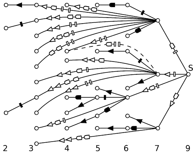
Figure 1: Branching tree of shapes for $3$ fermions in $3$ dimensions. The $36$ shapes are nodes, arranged in columns, with grade given below each column. The edges are decorated with operators whose action traverses the edge from right to left. The operators $\bar{T}$, $\bar{U}$ and $\bar{V}$ are depicted by graphically similar open symbols. The closed symbols analogously represent the operators $\underline{T\bar{T}}^{2}$, $\underline{U\bar{U}}^{2}$ and $\underline{V\bar{V}}^{2}$. All operators on a given edge are symmetrized together. For example, the shape at upper left is given by $\underline{V\bar{V}}^{2}\,\underline{\bar{V}\bar{U}\bar{T}}^{2}\,\underline{\bar{U}\bar{T}}\,S$, where $S$ is the source shape, depicted at far right. The dashed line is explained in the text.

The algorithm will now be described on the specific example of $3!^{2}=36$ shapes of $3$ particles in $3$ dimensions. In Fig. 1, the shapes are depicted as nodes in a graph, with the source shape $S=\Delta_{3}(t)\Delta_{3}(u)\Delta_{3}(v)$ on the right. Transformations of one shape into another are depicted by edges of the graph. These are effected by lowering operators, as denoted by edge decorations in the figure, giving the edges a natural orientation from right to left, also depicted by the orientation of the arrow-like symbols. Notably, a simple lowering operator like $\underline{\bar{T}}$ always gives zero when acting on any shape (cf. Proposition 5), so the elementary operators which lower the grade by one are $\underline{T\bar{T}}^{2}$ and similar, depicted by filled symbols. All shapes are generated from the source by lowering operators. One can imagine the operator symbols on the edges as filters, or funnels, which take the source flow from right to left, letting through shapes of ever lower grade.

2.6 Fermion sign problem

The three directions in space are equivalent, and so are the shift operators corresponding to them. Permutations of the shift operators in Fig. 1 give rise to different but equivalent graphs. The edges depicted by full lines form a particular kind of oriented spanning tree, where every node except the source (root of the tree) has exactly one incoming edge, while the root has none. Every choice of such a branching tree obviously fixes the phases of all shapes uniquely. It may be possible to add edges consistently with this sign choice, but this cannot be guaranteed in general. A conflicting insertion is depicted by the dashed line: in equations, it turns out that

$$\underline{\bar{V}\bar{T}}^{2}\,\underline{\bar{U}\bar{T}}\,S=-\underline{\bar{U}\bar{T}}^{2}\,\underline{\bar{V}\bar{T}}\,S.$$ (18)

This observation means that one cannot simply “turn loose” all possible operators on the source state to generate all possible shapes, because one will encounter the fermion sign problemLoh90 . In other words, a context-free, or local, definition of shape signs is not possible, because any algorithm changing the states will in principle allow some local moves which spoil the agreed-upon signs. Instead, the correct algorithmic definition of shape signs is a choice of branching tree rooted at the source, which is a global object.

In principle, simulations can deal with the above sign issue in one of three ways. The first is to generate all shapes beforehand and use them as a basis, while varying only the coefficients $\Phi_{i}$ in the simulation. This approach naturally leads to representing physical states as “vectors of symmetric polynomials,”

$$\left(\Phi_{1},\Phi_{2},\ldots,\Phi_{N!^{d-1}}\right).$$ (19)

Such a structure is called a free module (as distinct from a vector space, where the $\Phi_{i}$ would be just numbers). It evidently solves the sign problem, because states are mapped to a space of symmetric functions. The practicality of this proposal remains to be demonstrated.

Another possible approach is to compile a list of allowed operators, which are consistent with a given branching tree. These operators could then be used in a context-free manner, enabling one to generate shapes “on the fly” without storing them explicitly. It is an open question at present whether such a set of mutually consistent operators can always be found, which is also complete in the sense that they generate all the shapes.

Finally, one can try to find rules of calculation with the operators involved. In this approach, the individual shift operators are letters, while the symmetrized operators — underlined strings of one or more letters — are words. The task is to find the grammar of this language, a sort of extended Wick’s theorem. From this point of view, Eq. (18) looks as if the letters $\bar{T}$, $\bar{U}$ and $\bar{V}$ were anticommuting. The previous question of finding a complete consistent set of operators may now be rephrased: can one compile a list of words such that using them does not require a grammar? The formal-language approach is potentially the most powerful way to manipulate many-body states, but also requires the most future research.

3 Discussion

In the present work an efficient algorithm has been described, which generates all shapes of $N$ particles in odd dimensions. Much about the algorithm and especially the branching-tree structures it naturally engenders remains to be clarified. The discussion here places it in the broader context of efforts to represent fermion systems efficiently, concentrating on the open questions.

Most pragmatically, one can regard the algorithm as just another way to obtain shapes, more practical than the other known Sunko16-1 one, but in any case a means to an end. With the shapes in hand, the really interesting insight is to represent physical states as a free module (19), rather than a vector space. This is in some sense the furthest one can take Heisenberg’s matrix mechanics. It explains immediately why fermion systems cannot be directly bosonised in more than one dimension Tomonaga50 . Namely, in one dimension there is only one shape, the ground-state Slater determinant $\Psi_{0}$, so that any state can be written as $\Psi=\Phi\Psi_{0}$. Because $\Phi$ is a symmetric function, bosonisation succeeds: every excited state $\Psi$ is uniquely mapped on some boson wave function $\Phi$. In the standard second-quantized formalism, this result reads, say,

$$\left|\Psi\right>=B_{1}^{\dagger}B_{2}^{\dagger}\left|\Psi_{0}\right>\leftrightarrow\Phi_{1}\Phi_{2}\Psi_{0}=\Phi\Psi_{0}=\Psi,$$ (20)

for a given product of boson excitations. Because the free module (19) is one-dimensional in one dimension, the structure of excitations is purely multiplicative. Generally, however, the free module has dimension $N!^{d-1}$, so that excitations can be, for example,

$$B_{1}^{\dagger}\left|\Psi_{1}\right>+B_{2}^{\dagger}\left|\Psi_{2}\right>\leftrightarrow\Phi_{1}\Psi_{1}+\Phi_{2}\Psi_{2},$$ (21)

with same $B_{i}$’s (symmetric polynomials $\Phi_{i}$, or bosons) but different $\Psi_{i}$’s (shapes, or vacua). One can say either that bosonisation fails, because the structure of excitations is no longer multiplicative, or that it finally succeeds, because one has found the correct generalization of the one-dimensional case. In any case, the “deep” structure of fermionic excitations exposed here is that the vacua are like prime numbers, in the sense that they do not factorize: one cannot be obtained from another by multiplication. Therefore excitations must be described by a combination of multiplication and addition. As of this writing, it is of greatest interest to learn to calculate efficiently in the free module, because mapping fermionic states onto symmetric functions a priori solves the fermion sign problem.

The algorithm has an interesting feature from the theoretical point of view. All its moves reduce information, because they are net downshifts, which correspond to lowering monomial powers, reducing the overall degree of the polynomials involved. In order to go in the opposite direction, raising the degree, one would have to use quite “clever” combinations of upshifts in order to stay within the space of shapes, i.e. avoid states of the general form (1) with some $\Phi_{i}\neq 1$. In other words, upshifting requires adding information in order to make higher-grade shapes from lower-grade ones. It is like integration, while downshifting is like taking derivatives: one requires insight, while the other is an automatic operation. One must conclude that the source shape has the maximum information content, so that the “flow” passing through “filters” in Fig. 1 is the flow of information, or negentropy.

This conclusion runs quite counter to thermodynamic intuition, which takes for granted that states with high excitation energy have high entropy as well. The critical issue in this reasoning is the relationship between the number of nodes and the energy of the state. If the state is dominated by kinetic energy, one is in the weak-coupling limit, and the usual thermodynamic reasoning prevails. However, if it is dominated by correlations, the system may choose a “complicated” ground state, with more nodes, but unique in some sense, hence of low entropy. This situation is called strongly correlated, the most famous example being Hund’s rule Yamanaka05 .

The shape paradigm provides an interesting way to think about the strongly correlated limit. It is as if the system stays cold by using extra nodes to store information, in the form of some rare complicated states, instead of assigning nodes to kinetic motion, which would distribute them among a large number of common simple states, with high entropy. In particular, the source state is unique among a very large number of states with the same number of nodes. In our example of three particles in three dimensions, there are $3838$ states with nine nodes, only one of which is the source. In fact, mirroring indicates there must be a way to think of the source as a zero-entropy state, equivalent to the completely featureless boson ground state. Its concrete realization as a product of three one-dimensional fermionic ground states indicates the same.

A simple way to reconcile the above discussion with standard thermodynamics is to assign to each shape an entropy given by the logarithm of the coefficient of the shape polynomial, corresponding to its grade. This resolution has the pleasant property of specializing to the usual definition of entropy of the non-interacting ground state, which is just the logarithm of its degeneracy ($\ln 3$ in Fig. 1). The source shape always has zero entropy, just as the reasoning above indicated it should. In this way one can think of shapes as low-entropy states embedded in a much larger space of high-entropy ones. The latter are described by bosonic excitations of the shapes, as given by Eq. (1) with some $\Phi_{i}\neq 1$. In other words, the proper physical resolution of the above conundrum is that the shapes are a choice of possible vacua for a physical system, and these vacua are special in the sense that they have an exceptionally low entropy, or degeneracy, for their given energy. Once the ground state is selected, perhaps as a superposition of the vacua, the remaining shapes may still make their presence felt as bandheads of higher-energy excitation bands, such as are ubiquitous in the spectra of finite systems. In this way their “exceptionalism” persists, giving them a special role in the excitation spectrum, even if some other state is the ground state Sunko16-2 .

4 Conclusion

The shape paradigm has promise as both a theoretical and practical tool for the description of strongly correlated finite systems, particularly of fermions. While much remains to be done, the algorithm described in the present work removes a major roadblock in the practical application of the paradigm to transition-metal compounds, whose open $3d$ orbital requires that one should be able to manipulate states of around $N=5$ identical fermions. These materials are in the focus of current fundamental and applied interest, as both cuprate and pnictide high-temperature superconductors belong to this category. It is possible to separate the local (strongly correlated) part of the problem from the extended one Hyowon14 , making shapes an interesting contender for the description of the former. It is still too early for a direct comparison of the shape paradigm with other more mature approaches, or with experiment. Hopefully the readers will be motivated to join the exploration of shapes based on their own interests.

- (1) P. Lazić, D.K. Sunko, EPL (Europhysics Letters) 112(3), 37011 (2015). DOI 10.1209/0295-5075/112/37011
- (2) S.V. Borisenko, D.V. Evtushinsky, Z.H. Liu, I. Morozov, R. Kappenberger, S. Wurmehl, B. Buchner, A.N. Yaresko, T.K. Kim, M. Hoesch, T. Wolf, N.D. Zhigadlo, Nat Phys 12(4), 311 (2016). DOI 10.1038/nphys3594. Letter
- (3) H. Park, A.J. Millis, C.A. Marianetti, Phys. Rev. B 90, 235103 (2014). DOI 10.1103/PhysRevB.90.235103
- (4) G. Nikšić, I. Kupčić, D. Sunko, S. Barišić, Journal of Superconductivity and Novel Magnetism 26(8), 2669 (2013). DOI 10.1007/s10948-013-2157-9
- (5) O.S. Barišić, S. Barišić, J. Supercond. Nov. Magn. 25, 669 (2012). DOI 10.1007/s10948-012-1461-0
- (6) A. Bianconi, A.C. Castellano, M. De Santis, C. Politis, A. Marcelli, S. Mobilio, A. Savoia, Zeitschrift für Physik B Condensed Matter 67(3), 307 (1987). DOI 10.1007/BF01307254
- (7) J. Tahir-Kheli, W.A. Goddard, The Journal of Physical Chemistry Letters 2(18), 2326 (2011). DOI 10.1021/jz200916t
- (8) G. Campi, A. Ricci, N. Poccia, A. Bianconi, Journal of Superconductivity and Novel Magnetism 27(4), 987 (2014). DOI 10.1007/s10948-013-2434-7
- (9) G. Bianconi, Phys. Rev. E 85, 061113 (2012). DOI 10.1103/PhysRevE.85.061113
- (10) J. Tahir-Kheli, New Journal of Physics 15(7), 073020 (2013). DOI 10.1088/1367-2630/15/7/073020
- (11) S.I. Mirzaei, D. Stricker, J.N. Hancock, C. Berthod, A. Georges, E. van Heumen, M.K. Chan, X. Zhao, Y. Li, M. Greven, N. Barišić, D. van der Marel, PNAS 110(15), 5774 (2013). DOI 10.1073/pnas.1218846110
- (12) M.K. Chan, M.J. Veit, C.J. Dorow, Y. Ge, Y. Li, W. Tabis, Y. Tang, X. Zhao, N. Barišić, M. Greven, Phys. Rev. Lett. 113, 177005 (2014). DOI 10.1103/PhysRevLett.113.177005
- (13) A.P. Drozdov, M.I. Eremets, I.A. Troyan, V. Ksenofontov, S.I. Shylin, Nature 525(7567), 73 (2015). DOI 10.1038/nature14964. Letter
- (14) M. Einaga, M. Sakata, T. Ishikawa, K. Shimizu, M.I. Eremets, A.P. Drozdov, I.A. Troyan, N. Hirao, Y. Ohishi, Nat Phys advance online publication (2016). DOI 10.1038/nphys3760. Letter
- (15) A. Bussmann-Holder, J. Köhler, M.H. Whangbo, A. Bianconi, A. Simon, Novel Superconducting Materials 2, 37 (2016). DOI 10.1515/nsm-2016-0004
- (16) D.K. Sunko, Phys. Rev. A 93, 062109 (2016). DOI 10.1103/PhysRevA.93.062109
- (17) D.K. Sunko. Fundamental invariants of many-body Hilbert space (2016). Review article, submitted to Modern Physics Letters B.
- (18) H. Derksen, G. Kemper, Computational Invariant Theory (Springer Berlin Heidelberg, 2002)
- (19) E.Y. Loh, J.E. Gubernatis, R.T. Scalettar, S.R. White, D.J. Scalapino, R.L. Sugar, Phys. Rev. B 41, 9301 (1990). DOI 10.1103/PhysRevB.41.9301
- (20) S. Tomonaga, Progress of Theoretical Physics 5(4), 544 (1950). DOI 10.1143/ptp/5.4.544
- (21) S. Yamanaka, K. Koizumi, Y. Kitagawa, T. Kawakami, M. Okumura, K. Yamaguchi, International Journal of Quantum Chemistry 105(6), 687 (2005). DOI 10.1002/qua.20784