A Fast algorithm for Earth Mover’s Distance based on optimal transport and L1subscript𝐿1L_{1} type Regularization

Wuchen Li wcli@math.ucla.edu ,Β  Stanley Osher sjo@math.ucla.edu Β andΒ  Wilfrid Gangbo Department of Mathematics, University of California, Los Angeles.
Abstract.

We propose a new algorithm to approximate the Earth Mover’s distance (EMD). Our main idea is motivated by the theory of optimal transport, in which EMD can be reformulated as a familiar L1subscript𝐿1L_{1} type minimization. We use a regularization which gives us a unique solution for this L1subscript𝐿1L_{1} type problem. The new regularized minimization is very similar to problems which have been solved in the fields of compressed sensing and image processing, where several fast methods are available. In this paper, we adopt a primal-dual algorithm designed there, which uses very simple updates at each iteration and is shown to converge very rapidly. Several numerical examples are provided.

Key words and phrases:
Earth Mover’s distance; Optimal transport; Compressed sensing; Primal-dual algorithm; L1subscript𝐿1L_{1} regularization.
This work is partially supported by ONR grants N000141410683, N000141210838 and DOE grant DE-SC00183838.

1. Introduction

In this paper we propose a new algorithm to approximate the Earth Mover’s distance (EMD), which is motivated by the theory of optimal transport and methods related to those used in compressed sensing and image processing.

We begin by reviewing some well known facts. EMD, which is also named the Monge problem or the Wasserstein metric, plays a central role in many applications, including image processing, computer vision and statistics e.t.c [13, 16, 20, 25]. The EMD is a particular metric defined on the probability space of a convex, compact set Ξ©βŠ‚β„dΞ©superscriptℝ𝑑\Omega\subset\mathbb{R}^{d}. Given two probability densities ρ0superscript𝜌0\rho^{0}, ρ1superscript𝜌1\rho^{1} in a probability set 𝒫​(Ξ©)𝒫Ω\mathcal{P}(\Omega), where

𝒫​(Ξ©)={ρ​(x)∈L1​(Ξ©):βˆ«Ξ©Οβ€‹(x)​𝑑x=1,ρ​(x)β‰₯0}.𝒫Ωconditional-set𝜌π‘₯superscript𝐿1Ξ©formulae-sequencesubscriptΩ𝜌π‘₯differential-dπ‘₯1𝜌π‘₯0\mathcal{P}(\Omega)=\{\rho(x)\in L^{1}(\Omega)~{}:~{}\int_{\Omega}\rho(x)dx=1,\quad\rho(x)\geq 0\}\ .

The EMD deals with following (linear) minimization problem

E​M​D​(ρ0,ρ1):=minΟ€βˆ«Ξ©Γ—Ξ©d​(x,y)​π​(x,y)​𝑑x​𝑑yassign𝐸𝑀𝐷superscript𝜌0superscript𝜌1subscriptπœ‹subscriptΩΩ𝑑π‘₯π‘¦πœ‹π‘₯𝑦differential-dπ‘₯differential-d𝑦\begin{split}EMD(\rho^{0},\rho^{1}):=\min_{\pi}\quad\int_{\Omega\times\Omega}d(x,y)\pi(x,y)dxdy\end{split} (1)

with the constraint that the joint measure (also called the transport function) π​(x,y)πœ‹π‘₯𝑦\pi(x,y) has ρ0​(x)superscript𝜌0π‘₯\rho^{0}(x) and ρ1​(y)superscript𝜌1𝑦\rho^{1}(y) as marginals, i.e.

βˆ«Ξ©Ο€β€‹(x,y)​𝑑y=ρ0​(x),βˆ«Ξ©Ο€β€‹(x,y)​𝑑x=ρ1​(y),π​(x,y)β‰₯0.formulae-sequencesubscriptΞ©πœ‹π‘₯𝑦differential-d𝑦superscript𝜌0π‘₯formulae-sequencesubscriptΞ©πœ‹π‘₯𝑦differential-dπ‘₯superscript𝜌1π‘¦πœ‹π‘₯𝑦0\int_{\Omega}\pi(x,y)dy=\rho^{0}(x)\ ,\quad\int_{\Omega}\pi(x,y)dx=\rho^{1}(y)\ ,\quad\pi(x,y)\geq 0\ .

Here d𝑑d is a distance function on ℝdsuperscriptℝ𝑑\mathbb{R}^{d} which we call the ground metric. In this paper, we consider the ground metric either be the Euclidean distance (L2subscript𝐿2L_{2}) [4, 5] or the Manhattan distance (L1subscript𝐿1L_{1}) [15]. I.e. d​(x,y):=β€–xβˆ’yβ€–2assign𝑑π‘₯𝑦subscriptnormπ‘₯𝑦2d(x,y):=\|x-y\|_{2} or β€–xβˆ’yβ€–1subscriptnormπ‘₯𝑦1\|x-y\|_{1}. We call (1) with the L1subscript𝐿1L_{1}, L2subscript𝐿2L_{2} ground metric the EMD-L1subscript𝐿1L_{1}, EMD-L2subscript𝐿2L_{2}.

In recent years, (1) has been well studied by the theory of optimal transport [1, 9, 22, 26]. The theory (remarkably) points out that (1) is equivalent to a new minimization problem

E​M​D​(ρ0,ρ1)=infm{βˆ«Ξ©β€–m​(x)βˆ₯d​x:βˆ‡β‹…m​(x)+ρ1​(x)βˆ’Ο0​(x)=0},𝐸𝑀𝐷superscript𝜌0superscript𝜌1subscriptinfimumπ‘šconditional-setsubscriptΞ©:conditionalπ‘šπ‘₯𝑑π‘₯β‹…βˆ‡π‘šπ‘₯superscript𝜌1π‘₯superscript𝜌0π‘₯0EMD(\rho^{0},\rho^{1})=\inf_{m}\{\int_{\Omega}\|m(x)\|dx~{}:~{}\nabla\cdot m(x)+\rho^{1}(x)-\rho^{0}(x)=0\}\ , (2)

where βˆ₯β‹…βˆ₯\|\cdot\| is 222-norm (L2subscript𝐿2L_{2} ground metric) or 1-norm (L1subscript𝐿1L_{1} ground metric) in ℝdsuperscriptℝ𝑑\mathbb{R}^{d} and m:Ω→ℝd:π‘šβ†’Ξ©superscriptℝ𝑑m:~{}\Omega\rightarrow\mathbb{R}^{d} is a flux vector satisfying a zero flux condition. I.e. m​(x)⋅ν​(x)=0β‹…π‘šπ‘₯𝜈π‘₯0m(x)\cdot\nu(x)=0, where ν​(x)𝜈π‘₯\nu(x) is the unit normal vector for the boundary of ΩΩ\Omega.

The minimization (2) has an interesting fluid dynamics interpretation. It turns out that (2) can be viewed as the following optimal control problem

infρ,m{∫01βˆ«Ξ©β€–m​(t,x)βˆ₯d​x​d​t:βˆ‚Οβˆ‚t+βˆ‡β‹…m=0,ρ​(0)=ρ0,ρ​(1)=ρ1},subscriptinfimumπœŒπ‘šconditional-setsuperscriptsubscript01subscriptΞ©:conditionalπ‘šπ‘‘π‘₯𝑑π‘₯𝑑𝑑formulae-sequenceπœŒπ‘‘β‹…βˆ‡π‘š0formulae-sequence𝜌0superscript𝜌0𝜌1superscript𝜌1\inf_{\rho,m}\{\int_{0}^{1}\int_{\Omega}\|m(t,x)\|dxdt~{}:~{}\frac{\partial\rho}{\partial t}+\nabla\cdot m=0\ ,\quad\rho(0)=\rho^{0},\quad\rho(1)=\rho^{1}\ \}\ ,

where the minimum is taken among all possible flux functions m​(t,x)π‘šπ‘‘π‘₯m(t,x), such that the probability density function is moved continuously in time, from ρ0superscript𝜌0\rho^{0} to ρ1superscript𝜌1\rho^{1}. The optimal control problem has many minimizers. One of them is such that ρ​(t,x)=t​ρ1+(1βˆ’t)​ρ0πœŒπ‘‘π‘₯𝑑superscript𝜌11𝑑superscript𝜌0\rho(t,x)=t\rho^{1}+(1-t)\rho^{0}. Here the flux function m​(t,x)π‘šπ‘‘π‘₯m(t,x) does not depend on the time and βˆ‡β‹…m=βˆ’βˆ‚Οβˆ‚t=ρ0βˆ’Ο1β‹…βˆ‡π‘šπœŒπ‘‘superscript𝜌0superscript𝜌1\nabla\cdot m=-\frac{\partial\rho}{\partial t}=\rho^{0}-\rho^{1}, so that the control problem becomes (2), see [3, 10, 26] for details related to EMD-L2subscript𝐿2L_{2} and [8, 24] for similar optimal transport problems related to EMD-L1subscript𝐿1L_{1}.

The formulation (2) has two benefits numerically. First, the dimension in (2) is lower than the one in the original problem (1). Suppose we discretize ΩΩ\Omega by a grid with N𝑁N nodes. Since the unknown variable π​(x,y)πœ‹π‘₯𝑦\pi(x,y) in (1) is supported on Ω×ΩΩΩ\Omega\times\Omega and m​(x)π‘šπ‘₯m(x) in (1) only depends on ΩΩ\Omega, the number of grid points used in (2) is N𝑁N while the number needed in (1) is N2superscript𝑁2N^{2}. Second, (2) is an L1subscript𝐿1L_{1}-type minimization problem, which shares its structure with many problems in compressed sensing and image processing. It is possible to borrow a very fast and simple algorithm used there to solve EMD, see e.g. [11, 21, 27].

In this paper, we propose a new algorithm for EMD, leveraging the structure of the formulation (2). The algorithm mainly uses a finite volume method to discretize the domain ΩΩ\Omega and then applies the framework of primal-dual iterations designed in [7, 18]. We overcome the lack of strict convexity of (2) (EMD-L1subscript𝐿1L_{1}) by a regularization. Since the regularized minimization is a perturbation of a homogenous degree one minimization, our algorithm inherits all the benefits of the primal-dual algorithm: First, we use a shrink operator at each step, which handles the sparsity easily, see e.g. [11]; Second, the algorithm converges rapidly and each step involves very simple formulae. Thus the complexity of the algorithm is very low and the program is very simple.

EMD has been shown to be effective in applications [17] and many linear programming techniques have been proposed, see e.g. [12, 15] and many references therein. Recently, the authors in [4, 5, 25] used the Alternating Direction Method of Multipliers (ADMM), which can also solve the EMD with a general Finsler ground metric. We use the primal-dual algorithm rather than ADMM. So we do not need to solve an elliptic problem (i.e. the inverting of a Laplacian) and every iteration is explicit. Our updates are quite simple while ADMM might need fewer iterations. In addition, it is clear that the ADMM is difficult to parallelize while ours is quite easy. This means, with a parallel computer, the algorithm we propose can be made much faster. The primal-dual algorithm has been used before in optimal transport. The authors in [6] use it to compute the stationary solution of mean field games. However, the problem we consider is totally different. The emphasis of this paper is that we design simple and fast algorithms for EMD-L1subscript𝐿1L_{1}, EMD-L2subscript𝐿2L_{2}.

The outline of this paper is as follows. In section 2, we propose a primal-dual algorithm for (2) on a uniform grid. We analyze the algorithm in section 3. Several numerical examples are presented in section 4.

2. Algorithm

The EMD problem, as presented in (2), has similar structure to many homogenous degree one regularized problems. In this section we will use a finite volume discretization to approximate (2). The discretized problem becomes an L1subscript𝐿1L_{1}-type optimization with linear constraints, which allows us to apply the hybrid primal-dual method designed in [7, 18].

We begin with considering EMD-L2subscript𝐿2L_{2}. We shall consider a uniform lattice graph G=(V,E)𝐺𝑉𝐸G=(V,E) with spacing Δ​xΞ”π‘₯\Delta x to discretize the spatial domain, where V𝑉V is the vertex set

V={1,2,β‹―,N},𝑉12⋯𝑁V=\{1,2,\cdots,N\}\ ,

and E𝐸E is the edge set. Here i=(i1,β‹―,id)∈V𝑖subscript𝑖1β‹―subscript𝑖𝑑𝑉i=(i_{1},\cdots,i_{d})\in V represents a point in ℝdsuperscriptℝ𝑑\mathbb{R}^{d}.

We consider a discrete probability set supported on all vertices:

𝒫​(G)={(pi)i=1Nβˆˆβ„Nβˆ£βˆ‘i=1Npi=1,piβ‰₯0,i∈V},𝒫𝐺conditional-setsuperscriptsubscriptsubscript𝑝𝑖𝑖1𝑁superscriptℝ𝑁formulae-sequencesuperscriptsubscript𝑖1𝑁subscript𝑝𝑖1formulae-sequencesubscript𝑝𝑖0𝑖𝑉\mathcal{P}(G)=\{(p_{i})_{i=1}^{N}\in\mathbb{R}^{N}\mid\sum_{i=1}^{N}p_{i}=1\ ,~{}p_{i}\geq 0\ ,~{}i\in V\}\ ,

where pisubscript𝑝𝑖p_{i} represents a probability at node i𝑖i, i.e. pi=∫Ciρ​(x)​𝑑xsubscript𝑝𝑖subscriptsubscriptπΆπ‘–πœŒπ‘₯differential-dπ‘₯p_{i}=\int_{C_{i}}\rho(x)dx, Cisubscript𝐢𝑖C_{i} is a cube centered at i𝑖i with length Δ​xΞ”π‘₯\Delta x. So ρ0​(x)superscript𝜌0π‘₯\rho^{0}(x), ρ1​(x)superscript𝜌1π‘₯\rho^{1}(x) is approximated by p0=(pi0)i=1Nsuperscript𝑝0superscriptsubscriptsubscriptsuperscript𝑝0𝑖𝑖1𝑁p^{0}=(p^{0}_{i})_{i=1}^{N} and p1=(pi1)i=1Nsuperscript𝑝1superscriptsubscriptsubscriptsuperscript𝑝1𝑖𝑖1𝑁p^{1}=(p^{1}_{i})_{i=1}^{N}.

We use two steps to consider the EMD on 𝒫​(G)𝒫𝐺\mathcal{P}(G). We first define a flux on a lattice. Denote a matrix m=(mi+12)i=1Nβˆˆβ„NΓ—dπ‘šsuperscriptsubscriptsubscriptπ‘šπ‘–12𝑖1𝑁superscriptℝ𝑁𝑑m=(m_{i+\frac{1}{2}})_{i=1}^{N}\in\mathbb{R}^{N\times d}, where each component mi+12subscriptπ‘šπ‘–12m_{i+\frac{1}{2}} is a row vector in ℝdsuperscriptℝ𝑑\mathbb{R}^{d}, i.e.

mi+12=(mi+12​ev)v=1d=(∫Ci+12​evmv​(x)​𝑑x)v=1d,subscriptπ‘šπ‘–12superscriptsubscriptsubscriptπ‘šπ‘–12subscript𝑒𝑣𝑣1𝑑superscriptsubscriptsubscriptsubscript𝐢𝑖12subscript𝑒𝑣superscriptπ‘šπ‘£π‘₯differential-dπ‘₯𝑣1𝑑m_{i+\frac{1}{2}}=(m_{i+\frac{1}{2}e_{v}})_{v=1}^{d}=(\int_{C_{i+\frac{1}{2}e_{v}}}m^{v}(x)dx)_{v=1}^{d}\ ,

where ev=(0,β‹―,Δ​x,β‹―,0)Tsubscript𝑒𝑣superscript0β‹―Ξ”π‘₯β‹―0𝑇e_{v}=(0,\cdots,\Delta x,\cdots,0)^{T}, Δ​xΞ”π‘₯\Delta x is at the v𝑣v-th column. In other words, if we denote i=(i1,β‹―,id)βˆˆβ„d𝑖subscript𝑖1β‹―subscript𝑖𝑑superscriptℝ𝑑i=(i_{1},\cdots,i_{d})\in\mathbb{R}^{d} and m​(x)=(m1​(x),β‹―,md​(x))π‘šπ‘₯superscriptπ‘š1π‘₯β‹―superscriptπ‘šπ‘‘π‘₯m(x)=(m^{1}(x),\cdots,m^{d}(x)), then

mi+12​evβ‰ˆmv​(i1,β‹―,ivβˆ’1,iv+12​Δ​x,iv+1,β‹―,id)​Δ​xd.subscriptπ‘šπ‘–12subscript𝑒𝑣superscriptπ‘šπ‘£subscript𝑖1β‹―subscript𝑖𝑣1subscript𝑖𝑣12Ξ”π‘₯subscript𝑖𝑣1β‹―subscript𝑖𝑑Δsuperscriptπ‘₯𝑑m_{i+\frac{1}{2}e_{v}}\approx m^{v}(i_{1},\cdots,i_{v-1},i_{v}+\frac{1}{2}\Delta x,i_{v+1},\cdots,i_{d})\Delta x^{d}\ .

We consider a zero flux condition. So if a point i+12​ev𝑖12subscript𝑒𝑣i+\frac{1}{2}e_{v} is outside the domain ΩΩ\Omega, we let mi+12​ev=0subscriptπ‘šπ‘–12subscript𝑒𝑣0m_{i+\frac{1}{2}e_{v}}=0. Based on such a flux mπ‘šm, we define a discrete divergence operator divG​(m):=(divG​(mi))i=1NassignsubscriptdivπΊπ‘šsuperscriptsubscriptsubscriptdiv𝐺subscriptπ‘šπ‘–π‘–1𝑁\textrm{div}_{G}(m):=(\textrm{div}_{G}(m_{i}))_{i=1}^{N}, where

divG​(mi):=1Δ​xβ€‹βˆ‘v=1d(mi+12​evβˆ’miβˆ’12​ev).assignsubscriptdiv𝐺subscriptπ‘šπ‘–1Ξ”π‘₯superscriptsubscript𝑣1𝑑subscriptπ‘šπ‘–12subscript𝑒𝑣subscriptπ‘šπ‘–12subscript𝑒𝑣\textrm{div}_{G}(m_{i}):=\frac{1}{\Delta x}\sum_{v=1}^{d}(m_{i+\frac{1}{2}e_{v}}-m_{i-\frac{1}{2}e_{v}})\ .

We next introduce the discrete cost functional

β€–mβ€–:=βˆ‘i=1Nβ€–mi+12β€–2=βˆ‘i=1Nβˆ‘v=1d|mi+ev2|2.assignnormπ‘šsuperscriptsubscript𝑖1𝑁subscriptnormsubscriptπ‘šπ‘–122superscriptsubscript𝑖1𝑁superscriptsubscript𝑣1𝑑superscriptsubscriptπ‘šπ‘–subscript𝑒𝑣22\|m\|:=\sum_{i=1}^{N}\|m_{i+\frac{1}{2}}\|_{2}=\sum_{i=1}^{N}\sqrt{\sum_{v=1}^{d}|m_{i+\frac{e_{v}}{2}}|^{2}}\ .

To summarize, (2) forms an optimization problem

minimizeπ‘šπ‘šminimize\displaystyle\underset{m}{\text{minimize}} β€–mβ€–normπ‘š\displaystyle\|m\|
subject to divG​(m)+p1βˆ’p0=0,subscriptdivπΊπ‘šsuperscript𝑝1superscript𝑝00\displaystyle\textrm{div}_{G}(m)+p^{1}-p^{0}=0\ ,

which can be written explicitly as

minimizeπ‘šπ‘šminimize\displaystyle\underset{m}{\text{minimize}} βˆ‘i=1Nβˆ‘v=1d|mi+ev2|2superscriptsubscript𝑖1𝑁superscriptsubscript𝑣1𝑑superscriptsubscriptπ‘šπ‘–subscript𝑒𝑣22\displaystyle\sum_{i=1}^{N}\sqrt{\sum_{v=1}^{d}|m_{i+\frac{e_{v}}{2}}|^{2}} (3)
subject to 1Δ​xβ€‹βˆ‘v=1d(mi+12​evβˆ’miβˆ’12​ev)+pi1βˆ’pi0=0,i=1,β‹―,N,v=1,β‹―,d.formulae-sequence1Ξ”π‘₯superscriptsubscript𝑣1𝑑subscriptπ‘šπ‘–12subscript𝑒𝑣subscriptπ‘šπ‘–12subscript𝑒𝑣superscriptsubscript𝑝𝑖1superscriptsubscript𝑝𝑖00formulae-sequence𝑖1⋯𝑁𝑣1⋯𝑑\displaystyle\frac{1}{\Delta x}\sum_{v=1}^{d}(m_{i+\frac{1}{2}e_{v}}-m_{i-\frac{1}{2}e_{v}})+p_{i}^{1}-p_{i}^{0}=0\ ,\quad i=1,\cdots,N,~{}v=1,\cdots,d\ .

We observe that (3) is an optimization problem, which is very similar to some problems in compressed sensing and image processing e.g. [11], whose cost functional is convex and whose constraints are linear. Thus we solve (3) by looking at its saddle point structure. Denote Ξ¦=(Ξ¦i)i=1NΞ¦superscriptsubscriptsubscriptΦ𝑖𝑖1𝑁\Phi=(\Phi_{i})_{i=1}^{N} as (3)’s Lagrange multiplier, thus we have

minm⁑maxΞ¦L​(m,Ξ¦):=minm⁑maxΞ¦β€–mβ€–+Ξ¦T​(divG​(m)+p1βˆ’p0).formulae-sequenceassignsubscriptπ‘šsubscriptΞ¦πΏπ‘šΞ¦subscriptπ‘šsubscriptΞ¦normπ‘šsuperscriptΦ𝑇subscriptdivπΊπ‘šsuperscript𝑝1superscript𝑝0\min_{m}\max_{\Phi}\quad L(m,\Phi):=\min_{m}\max_{\Phi}\quad\|m\|+\Phi^{T}(\textrm{div}_{G}(m)+p^{1}-p^{0})\ . (4)

Saddle point problems, such as (4), are well studied by the first order primal-dual algorithm [7, 18]. The iteration steps are as follows:

{mk+1=arg⁑minm⁑‖mβ€–+(Ξ¦k)T​divG​(m)+β€–mβˆ’mkβ€–222​μ;Ξ¦k+1=arg⁑maxΦ⁑ΦT​(divG​(mk+1+θ​(mk+1βˆ’mk))+p1βˆ’p0)βˆ’β€–Ξ¦βˆ’Ξ¦kβ€–222​τ,casessuperscriptπ‘šπ‘˜1absentsubscriptπ‘šnormπ‘šsuperscriptsuperscriptΞ¦π‘˜π‘‡subscriptdivπΊπ‘šsubscriptsuperscriptnormπ‘šsuperscriptπ‘šπ‘˜222πœ‡superscriptΞ¦π‘˜1absentsubscriptΞ¦superscriptΦ𝑇subscriptdiv𝐺superscriptπ‘šπ‘˜1πœƒsuperscriptπ‘šπ‘˜1superscriptπ‘šπ‘˜superscript𝑝1superscript𝑝0subscriptsuperscriptnormΞ¦superscriptΞ¦π‘˜222𝜏\begin{cases}m^{k+1}=&\arg\min_{m}\|m\|+(\Phi^{k})^{T}\textrm{div}_{G}(m)+\frac{\|m-m^{k}\|^{2}_{2}}{2\mu}\ ;\\ \Phi^{k+1}=&\arg\max_{\Phi}\Phi^{T}\big{(}\textrm{div}_{G}(m^{k+1}+\theta(m^{k+1}-m^{k}))+p^{1}-p^{0}\big{)}-\frac{\|\Phi-\Phi^{k}\|^{2}_{2}}{2\tau}\ ,\end{cases} (5)

where ΞΌπœ‡\mu, Ο„πœ\tau are two small step sizes, θ∈[0,1]πœƒ01\theta\in[0,1] is a given parameter, β€–mβˆ’mkβ€–22=βˆ‘i=1Nβˆ‘v=1d(mi+12​evβˆ’mi+12​evk)2subscriptsuperscriptnormπ‘šsuperscriptπ‘šπ‘˜22superscriptsubscript𝑖1𝑁superscriptsubscript𝑣1𝑑superscriptsubscriptπ‘šπ‘–12subscript𝑒𝑣superscriptsubscriptπ‘šπ‘–12subscriptπ‘’π‘£π‘˜2\|m-m^{k}\|^{2}_{2}=\sum_{i=1}^{N}\sum_{v=1}^{d}(m_{i+\frac{1}{2}e_{v}}-m_{i+\frac{1}{2}e_{v}}^{k})^{2} and β€–Ξ¦βˆ’Ξ¦kβ€–22=βˆ‘i=1N(Ξ¦iβˆ’Ξ¦ik)2subscriptsuperscriptnormΞ¦superscriptΞ¦π‘˜22superscriptsubscript𝑖1𝑁superscriptsubscriptΦ𝑖superscriptsubscriptΞ¦π‘–π‘˜2\|\Phi-\Phi^{k}\|^{2}_{2}=\sum_{i=1}^{N}(\Phi_{i}-\Phi_{i}^{k})^{2}. These steps are alternating a gradient ascent in the dual variable ΦΦ\Phi and a gradient descent in the primal variable mπ‘šm.

It turns out that iteration (5) can be solved by simple explicit formulae. Since the unknown variable mπ‘šm, ΦΦ\Phi is component-wise separable in this problem, each of its components mi+12subscriptπ‘šπ‘–12m_{i+\frac{1}{2}}, Ξ¦isubscriptΦ𝑖\Phi_{i} can be independently obtained by solving (5).

First, notice

minm⁑‖mβ€–+(Ξ¦k)T​divG​(m)+β€–mβˆ’mkβ€–222​μ=minmβ€‹βˆ‘i=1Nβˆ‘v=1dmi+ev22+1Δ​xβ€‹βˆ‘i=1Nβˆ‘v=1dΞ¦ik​(mi+12​evβˆ’miβˆ’12​ev)+β€–mβˆ’mkβ€–222​μ=βˆ‘i=1Nminmi+12⁑(β€–mi+12β€–2βˆ’(βˆ‡GΞ¦i+12k)T​mi+12+12​μ​‖mi+12βˆ’mi+12kβ€–22),subscriptπ‘šdelimited-βˆ₯βˆ₯π‘šsuperscriptsuperscriptΞ¦π‘˜π‘‡subscriptdivπΊπ‘šsubscriptsuperscriptnormπ‘šsuperscriptπ‘šπ‘˜222πœ‡subscriptπ‘šsuperscriptsubscript𝑖1𝑁superscriptsubscript𝑣1𝑑superscriptsubscriptπ‘šπ‘–subscript𝑒𝑣221Ξ”π‘₯superscriptsubscript𝑖1𝑁superscriptsubscript𝑣1𝑑superscriptsubscriptΞ¦π‘–π‘˜subscriptπ‘šπ‘–12subscript𝑒𝑣subscriptπ‘šπ‘–12subscript𝑒𝑣subscriptsuperscriptnormπ‘šsuperscriptπ‘šπ‘˜222πœ‡superscriptsubscript𝑖1𝑁subscriptsubscriptπ‘šπ‘–12subscriptdelimited-βˆ₯βˆ₯subscriptπ‘šπ‘–122superscriptsubscriptβˆ‡πΊsuperscriptsubscriptΦ𝑖12π‘˜π‘‡subscriptπ‘šπ‘–1212πœ‡subscriptsuperscriptdelimited-βˆ₯βˆ₯subscriptπ‘šπ‘–12superscriptsubscriptπ‘šπ‘–12π‘˜22\begin{split}&\min_{m}~{}\|m\|+(\Phi^{k})^{T}\textrm{div}_{G}(m)+\frac{\|m-m^{k}\|^{2}_{2}}{2\mu}\\ =&\min_{m}\sum_{i=1}^{N}\sum_{v=1}^{d}\sqrt{m_{i+\frac{e_{v}}{2}}^{2}}+\frac{1}{\Delta x}\sum_{i=1}^{N}\sum_{v=1}^{d}\Phi_{i}^{k}(m_{i+\frac{1}{2}e_{v}}-m_{i-\frac{1}{2}e_{v}})+\frac{\|m-m^{k}\|^{2}_{2}}{2\mu}\\ =&\sum_{i=1}^{N}\min_{m_{i+\frac{1}{2}}}\big{(}\|m_{i+\frac{1}{2}}\|_{2}-(\nabla_{G}\Phi_{i+\frac{1}{2}}^{k})^{T}m_{i+\frac{1}{2}}+\frac{1}{2\mu}\|m_{i+\frac{1}{2}}-m_{i+\frac{1}{2}}^{k}\|^{2}_{2}\big{)}\ ,\end{split}

where βˆ‡GΞ¦i+12k:=1Δ​x​(Ξ¦i+evkβˆ’Ξ¦ik)v=1dassignsubscriptβˆ‡πΊsubscriptsuperscriptΞ¦π‘˜π‘–121Ξ”π‘₯superscriptsubscriptsubscriptsuperscriptΞ¦π‘˜π‘–subscript𝑒𝑣superscriptsubscriptΞ¦π‘–π‘˜π‘£1𝑑\nabla_{G}\Phi^{k}_{i+\frac{1}{2}}:=\frac{1}{\Delta x}(\Phi^{k}_{i+e_{v}}-\Phi_{i}^{k})_{v=1}^{d}. The first iteration in (5) has an explicit solution, which is:

mi+12k+1=shrink2​(mi+12k+ΞΌβ€‹βˆ‡GΞ¦i+12k,ΞΌ),subscriptsuperscriptπ‘šπ‘˜1𝑖12subscriptshrink2superscriptsubscriptπ‘šπ‘–12π‘˜πœ‡subscriptβˆ‡πΊsubscriptsuperscriptΞ¦π‘˜π‘–12πœ‡m^{k+1}_{i+\frac{1}{2}}=\textrm{shrink}_{2}(m_{i+\frac{1}{2}}^{k}+\mu\nabla_{G}\Phi^{k}_{i+\frac{1}{2}},\mu)\ ,

where we define the shrink2subscriptshrink2\textrm{shrink}_{2} operation

shrink2​(y,Ξ±):=yβ€–yβ€–2​max⁑{β€–yβ€–2βˆ’Ξ±,0},whereΒ yβˆˆβ„dΒ .assignsubscriptshrink2𝑦𝛼𝑦subscriptnorm𝑦2subscriptnorm𝑦2𝛼0whereΒ yβˆˆβ„dΒ .\textrm{shrink}_{2}(y,\alpha):=\frac{y}{\|y\|_{2}}\max\{\|y\|_{2}-\alpha,0\}\ ,\quad\textrm{where $y\in\mathbb{R}^{d}$\ .}

Second, consider

maxΦ⁑ΦT​divG​(mk+1+θ​(mk+1βˆ’mk))βˆ’β€–Ξ¦βˆ’Ξ¦kβ€–222​τ=βˆ‘i=1NmaxΞ¦i⁑{Ξ¦i​[divG​(mik+1+θ​(mik+1βˆ’mik))+pi1βˆ’pi0]βˆ’β€–Ξ¦iβˆ’Ξ¦ikβ€–222​τ}.subscriptΞ¦superscriptΦ𝑇subscriptdiv𝐺superscriptπ‘šπ‘˜1πœƒsuperscriptπ‘šπ‘˜1superscriptπ‘šπ‘˜subscriptsuperscriptnormΞ¦superscriptΞ¦π‘˜222𝜏superscriptsubscript𝑖1𝑁subscriptsubscriptΦ𝑖subscriptΦ𝑖delimited-[]subscriptdiv𝐺superscriptsubscriptπ‘šπ‘–π‘˜1πœƒsubscriptsuperscriptπ‘šπ‘˜1𝑖subscriptsuperscriptπ‘šπ‘˜π‘–superscriptsubscript𝑝𝑖1superscriptsubscript𝑝𝑖0subscriptsuperscriptnormsubscriptΦ𝑖subscriptsuperscriptΞ¦π‘˜π‘–222𝜏\begin{split}&\max_{\Phi}\Phi^{T}\textrm{div}_{G}(m^{k+1}+\theta(m^{k+1}-m^{k}))-\frac{\|\Phi-\Phi^{k}\|^{2}_{2}}{2\tau}\\ =&\sum_{i=1}^{N}\max_{\Phi_{i}}\big{\{}\Phi_{i}[\textrm{div}_{G}(m_{i}^{k+1}+\theta(m^{k+1}_{i}-m^{k}_{i}))+p_{i}^{1}-p_{i}^{0}]-\frac{\|\Phi_{i}-\Phi^{k}_{i}\|^{2}_{2}}{2\tau}\big{\}}\ .\\ \end{split}

Thus the second iteration in (5) becomes

Ξ¦ik+1=Ξ¦ik+τ​{divG​(mik+1+θ​(mik+1βˆ’mik))+pi1βˆ’pi0}.superscriptsubscriptΞ¦π‘–π‘˜1superscriptsubscriptΞ¦π‘–π‘˜πœsubscriptdiv𝐺superscriptsubscriptπ‘šπ‘–π‘˜1πœƒsubscriptsuperscriptπ‘šπ‘˜1𝑖subscriptsuperscriptπ‘šπ‘˜π‘–superscriptsubscript𝑝𝑖1subscriptsuperscript𝑝0𝑖\Phi_{i}^{k+1}=\Phi_{i}^{k}+\tau\big{\{}\textrm{div}_{G}(m_{i}^{k+1}+\theta(m^{k+1}_{i}-m^{k}_{i}))+p_{i}^{1}-p^{0}_{i}\}\ .

We are now ready to state our algorithm.

Β 
Primal-Dual for EMD-L2subscript𝐿2L_{2}
Input: Discrete probabilities p0superscript𝑝0p^{0}, p1superscript𝑝1p^{1};
Initial guess of m0superscriptπ‘š0m^{0}, step size ΞΌπœ‡\mu, Ο„πœ\tau, θ∈[0,1]πœƒ01\theta\in[0,1].
Output: mπ‘šm and EMD value β€–mβ€–normπ‘š\|m\|.
Β 
1. for k=1,2,β‹―π‘˜12β‹―k=1,2,\cdots   Iterates until convergence
2. mi+12k+1=shrink2​(mi+12k+ΞΌβ€‹βˆ‡GΞ¦i+12k,ΞΌ)subscriptsuperscriptπ‘šπ‘˜1𝑖12subscriptshrink2superscriptsubscriptπ‘šπ‘–12π‘˜πœ‡subscriptβˆ‡πΊsubscriptsuperscriptΞ¦π‘˜π‘–12πœ‡m^{k+1}_{i+\frac{1}{2}}=\textrm{shrink}_{2}(m_{i+\frac{1}{2}}^{k}+\mu\nabla_{G}\Phi^{k}_{i+\frac{1}{2}},\mu) ;
3. Ξ¦ik+1=Ξ¦ik+τ​{divG​(mik+1+θ​(mik+1βˆ’mik))+pi1βˆ’pi0}superscriptsubscriptΞ¦π‘–π‘˜1superscriptsubscriptΞ¦π‘–π‘˜πœsubscriptdiv𝐺superscriptsubscriptπ‘šπ‘–π‘˜1πœƒsubscriptsuperscriptπ‘šπ‘˜1𝑖subscriptsuperscriptπ‘šπ‘˜π‘–superscriptsubscript𝑝𝑖1subscriptsuperscript𝑝0𝑖\Phi_{i}^{k+1}=\Phi_{i}^{k}+\tau\{\textrm{div}_{G}(m_{i}^{k+1}+\theta(m^{k+1}_{i}-m^{k}_{i}))+p_{i}^{1}-p^{0}_{i}\} ;
4. end
Β 

We next consider EMD-L1subscript𝐿1L_{1}. Similarly, (2) forms the following optimization problem

minimizeπ‘šπ‘šminimize\displaystyle\underset{m}{\text{minimize}} β€–mβ€–1subscriptnormπ‘š1\displaystyle\|m\|_{1}
subject to divG​(m)+p1βˆ’p0=0,subscriptdivπΊπ‘šsuperscript𝑝1superscript𝑝00\displaystyle\textrm{div}_{G}(m)+p^{1}-p^{0}=0\ ,

which can be written explicitly as

minimizeπ‘šπ‘šminimize\displaystyle\underset{m}{\text{minimize}} βˆ‘i=1Nβˆ‘v=1d|mi+ev2|superscriptsubscript𝑖1𝑁superscriptsubscript𝑣1𝑑subscriptπ‘šπ‘–subscript𝑒𝑣2\displaystyle\sum_{i=1}^{N}\sum_{v=1}^{d}|m_{i+\frac{e_{v}}{2}}| (6)
subject to 1Δ​xβ€‹βˆ‘v=1d(mi+ev2βˆ’miβˆ’ev2)+pi1βˆ’pi0=0,i=1,β‹―,n,v=1,β‹―,d.formulae-sequence1Ξ”π‘₯superscriptsubscript𝑣1𝑑subscriptπ‘šπ‘–subscript𝑒𝑣2subscriptπ‘šπ‘–subscript𝑒𝑣2superscriptsubscript𝑝𝑖1superscriptsubscript𝑝𝑖00formulae-sequence𝑖1⋯𝑛𝑣1⋯𝑑\displaystyle\frac{1}{\Delta x}\sum_{v=1}^{d}(m_{i+\frac{e_{v}}{2}}-m_{i-\frac{e_{v}}{2}})+p_{i}^{1}-p_{i}^{0}=0\ ,\quad i=1,\cdots,n\ ,~{}v=1,\cdots,d\ .

We observe that (6) is an L1subscript𝐿1L_{1} optimization problem, whose cost function is convex and whose constraints are linear. However, the cost functional in (6) is not strictly convex, which often implies the existence of multiple minimizers. To deal with this issue, we consider a small quadratic perturbation, through which we pick up a unique solution for a modified problem:

minimizeπ‘šπ‘šminimize\displaystyle\underset{m}{\text{minimize}} β€–mβ€–1+Ο΅2​‖mβ€–22subscriptnormπ‘š1italic-Ο΅2superscriptsubscriptnormπ‘š22\displaystyle\|m\|_{1}+\frac{\epsilon}{2}\|m\|_{2}^{2} (7)
subject to divG​(m)+p1βˆ’p0=0.subscriptdivπΊπ‘šsuperscript𝑝1superscript𝑝00\displaystyle\textrm{div}_{G}(m)+p^{1}-p^{0}=0\ .

Here β€–mβ€–22=βˆ‘i=1Nβˆ‘v=1dmi+ev22superscriptsubscriptnormπ‘š22superscriptsubscript𝑖1𝑁superscriptsubscript𝑣1𝑑superscriptsubscriptπ‘šπ‘–subscript𝑒𝑣22\|m\|_{2}^{2}=\sum_{i=1}^{N}\sum_{v=1}^{d}m_{i+\frac{e_{v}}{2}}^{2} and Ο΅italic-Ο΅\epsilon is a positive scalar.

From now on, we solve (7) by looking at its saddle point structure. Denote Ξ¦=(Ξ¦i)i=1NΞ¦superscriptsubscriptsubscriptΦ𝑖𝑖1𝑁\Phi=(\Phi_{i})_{i=1}^{N} as (7)’s Lagrange multiplier, we have

minm⁑maxΞ¦L​(m,Ξ¦):=minm⁑maxΦ⁑‖mβ€–1+Ο΅2​‖mβ€–22+Ξ¦T​(divG​(m)+p1βˆ’p0).assignsubscriptπ‘šsubscriptΞ¦πΏπ‘šΞ¦subscriptπ‘šsubscriptΞ¦subscriptnormπ‘š1italic-Ο΅2superscriptsubscriptnormπ‘š22superscriptΦ𝑇subscriptdivπΊπ‘šsuperscript𝑝1superscript𝑝0\min_{m}\max_{\Phi}\quad L(m,\Phi):=\min_{m}\max_{\Phi}~{}\|m\|_{1}+\frac{\epsilon}{2}\|m\|_{2}^{2}+\Phi^{T}(\textrm{div}_{G}(m)+p^{1}-p^{0})\ . (8)

Since L​(β‹…,Ξ¦)𝐿⋅ΦL(\cdot,\Phi) is strictly convex which grows quadratically, and L​(m,β‹…)πΏπ‘šβ‹…L(m,\cdot) is linear, L𝐿L admits a saddle point solution. Again, we solve (8) by the first order primal-dual algorithm [7, 18]. The iteration steps are as follows:

{mk+1=arg⁑minm⁑‖mβ€–1+Ο΅2​‖mβ€–22+(Ξ¦k)T​divG​(m)+β€–mβˆ’mkβ€–222​μ;Ξ¦k+1=arg⁑maxΦ⁑ΦT​divG​(mk+1+θ​(mk+1βˆ’mk)+pi1βˆ’pi0)βˆ’β€–Ξ¦βˆ’Ξ¦kβ€–222​τ.casessuperscriptπ‘šπ‘˜1absentsubscriptπ‘šsubscriptnormπ‘š1italic-Ο΅2superscriptsubscriptnormπ‘š22superscriptsuperscriptΞ¦π‘˜π‘‡subscriptdivπΊπ‘šsubscriptsuperscriptnormπ‘šsuperscriptπ‘šπ‘˜222πœ‡superscriptΞ¦π‘˜1absentsubscriptΞ¦superscriptΦ𝑇subscriptdiv𝐺superscriptπ‘šπ‘˜1πœƒsuperscriptπ‘šπ‘˜1superscriptπ‘šπ‘˜subscriptsuperscript𝑝1𝑖subscriptsuperscript𝑝0𝑖subscriptsuperscriptnormΞ¦superscriptΞ¦π‘˜222𝜏\begin{cases}m^{k+1}=&\arg\min_{m}\|m\|_{1}+\frac{\epsilon}{2}\|m\|_{2}^{2}+(\Phi^{k})^{T}\textrm{div}_{G}(m)+\frac{\|m-m^{k}\|^{2}_{2}}{2\mu}\ ;\\ \Phi^{k+1}=&\arg\max_{\Phi}\Phi^{T}\textrm{div}_{G}(m^{k+1}+\theta(m^{k+1}-m^{k})+p^{1}_{i}-p^{0}_{i})-\frac{\|\Phi-\Phi^{k}\|^{2}_{2}}{2\tau}\ .\end{cases} (9)

As in the computation of EMD-L2subscript𝐿2L_{2}, we use simple exact formulae for (9). First, the update for mk+1superscriptπ‘šπ‘˜1m^{k+1} has explicit solution, which acts separately on each component mi+ev2k+1subscriptsuperscriptπ‘šπ‘˜1𝑖subscript𝑒𝑣2m^{k+1}_{i+\frac{e_{v}}{2}}:

minm⁑‖mβ€–1+Ο΅2​‖mβ€–22+(Ξ¦k)T​divG​(m)+β€–mβˆ’mkβ€–222​μ=minmβ€‹βˆ‘i=1Nβˆ‘v=1d{|mi+ev2|+Ο΅2​mi+ev22+1Δ​x​Φik​(mi+ev2βˆ’miβˆ’ev2)+(mi+ev2βˆ’mi+ev2k)22​μ}=βˆ‘i=1Nβˆ‘v=1dminmi+ev2⁑{|mi+ev2|+Ο΅2​mi+ev22βˆ’βˆ‡GΞ¦i+ev2k​mi+ev2+12​μ​(mi+ev2βˆ’mi+ev2k)2},subscriptπ‘šsubscriptdelimited-βˆ₯βˆ₯π‘š1italic-Ο΅2superscriptsubscriptdelimited-βˆ₯βˆ₯π‘š22superscriptsuperscriptΞ¦π‘˜π‘‡subscriptdivπΊπ‘šsubscriptsuperscriptnormπ‘šsuperscriptπ‘šπ‘˜222πœ‡subscriptπ‘šsuperscriptsubscript𝑖1𝑁superscriptsubscript𝑣1𝑑subscriptπ‘šπ‘–subscript𝑒𝑣2italic-Ο΅2superscriptsubscriptπ‘šπ‘–subscript𝑒𝑣221Ξ”π‘₯superscriptsubscriptΞ¦π‘–π‘˜subscriptπ‘šπ‘–subscript𝑒𝑣2subscriptπ‘šπ‘–subscript𝑒𝑣2superscriptsubscriptπ‘šπ‘–subscript𝑒𝑣2subscriptsuperscriptπ‘šπ‘˜π‘–subscript𝑒𝑣222πœ‡superscriptsubscript𝑖1𝑁superscriptsubscript𝑣1𝑑subscriptsubscriptπ‘šπ‘–subscript𝑒𝑣2subscriptπ‘šπ‘–subscript𝑒𝑣2italic-Ο΅2superscriptsubscriptπ‘šπ‘–subscript𝑒𝑣22subscriptβˆ‡πΊsubscriptsuperscriptΞ¦π‘˜π‘–subscript𝑒𝑣2subscriptπ‘šπ‘–subscript𝑒𝑣212πœ‡superscriptsubscriptπ‘šπ‘–subscript𝑒𝑣2superscriptsubscriptπ‘šπ‘–subscript𝑒𝑣2π‘˜2\begin{split}&\min_{m}~{}\|m\|_{1}+\frac{\epsilon}{2}\|m\|_{2}^{2}+(\Phi^{k})^{T}\textrm{div}_{G}(m)+\frac{\|m-m^{k}\|^{2}_{2}}{2\mu}\\ =&\min_{m}\sum_{i=1}^{N}\sum_{v=1}^{d}\big{\{}|m_{i+\frac{e_{v}}{2}}|+\frac{\epsilon}{2}m_{i+\frac{e_{v}}{2}}^{2}+\frac{1}{\Delta x}\Phi_{i}^{k}(m_{i+\frac{e_{v}}{2}}-m_{i-\frac{e_{v}}{2}})+\frac{(m_{i+\frac{e_{v}}{2}}-m^{k}_{i+\frac{e_{v}}{2}})^{2}}{2\mu}\big{\}}\\ =&\sum_{i=1}^{N}\sum_{v=1}^{d}\min_{m_{i+\frac{e_{v}}{2}}}\big{\{}|m_{i+\frac{e_{v}}{2}}|+\frac{\epsilon}{2}m_{i+\frac{e_{v}}{2}}^{2}-\nabla_{G}\Phi^{k}_{i+\frac{e_{v}}{2}}m_{i+\frac{e_{v}}{2}}+\frac{1}{2\mu}(m_{i+\frac{e_{v}}{2}}-m_{i+\frac{e_{v}}{2}}^{k})^{2}\big{\}}\ ,\end{split}

where βˆ‡GΞ¦i+ev2k:=1Δ​x​(Ξ¦i+evkβˆ’Ξ¦ik)assignsubscriptβˆ‡πΊsubscriptsuperscriptΞ¦π‘˜π‘–subscript𝑒𝑣21Ξ”π‘₯subscriptsuperscriptΞ¦π‘˜π‘–subscript𝑒𝑣subscriptsuperscriptΞ¦π‘˜π‘–\nabla_{G}\Phi^{k}_{i+\frac{e_{v}}{2}}:=\frac{1}{\Delta x}(\Phi^{k}_{i+e_{v}}-\Phi^{k}_{i}). So the first iteration in (9) has an explicit solution:

mi+ev2k+1=11+ϡ​μ​shrink​(mi+ev2k+ΞΌβ€‹βˆ‡GΞ¦i+ev2k,ΞΌ),subscriptsuperscriptπ‘šπ‘˜1𝑖subscript𝑒𝑣211italic-Ο΅πœ‡shrinksuperscriptsubscriptπ‘šπ‘–subscript𝑒𝑣2π‘˜πœ‡subscriptβˆ‡πΊsubscriptsuperscriptΞ¦π‘˜π‘–subscript𝑒𝑣2πœ‡m^{k+1}_{i+\frac{e_{v}}{2}}=\frac{1}{1+\epsilon\mu}\textrm{shrink}(m_{i+\frac{e_{v}}{2}}^{k}+\mu\nabla_{G}\Phi^{k}_{i+\frac{e_{v}}{2}},\mu)\ ,

where we define a shrink operation in ℝ1superscriptℝ1\mathbb{R}^{1}

shrink​(y,Ξ±):=sign⁑(y)​max⁑{|y|βˆ’Ξ±,0}={yβˆ’Ξ±ifΒ y>Ξ±Β ;0ifΒ βˆ’a≀y≀α ;y+Ξ±ifΒ y<βˆ’Ξ±Β .assignshrink𝑦𝛼sign𝑦𝑦𝛼0cases𝑦𝛼ifΒ y>Ξ±Β ;0ifΒ βˆ’a≀y≀α ;𝑦𝛼ifΒ y<βˆ’Ξ±Β .\textrm{shrink}(y,\alpha):=\operatorname{\mathrm{sign}}(y)\max\{|y|-\alpha,0\}=\begin{cases}y-\alpha\quad&\textrm{if $y>\alpha$\ ;}\\ 0\quad&\textrm{if $-a\leq y\leq\alpha$\ ;}\\ y+\alpha\quad&\textrm{if $y<-\alpha$\ .}\end{cases}

Second, the update for Ξ¦k+1superscriptΞ¦π‘˜1\Phi^{k+1} is same as the one in EMD-L2subscript𝐿2L_{2}. Since the second iteration in (9) is identical to the one in (5).

Β 
Primal-dual method for EMDβˆ’L1EMDsubscript𝐿1\textrm{EMD}-L_{1}
Input: Discrete probabilities p0superscript𝑝0p^{0}, p1superscript𝑝1p^{1};
Initial guess of m0superscriptπ‘š0m^{0}, parameter Ο΅>0italic-Ο΅0\epsilon>0, step size ΞΌπœ‡\mu, Ο„πœ\tau, θ∈[0,1]πœƒ01\theta\in[0,1].
Output: mπ‘šm and EMD value β€–mβ€–1subscriptnormπ‘š1\|m\|_{1}.
Β 
1. for k=1,2,β‹―π‘˜12β‹―k=1,2,\cdots   Iterates until convergence
2. mi+ev2k+1=11+ϡ​μ​shrink​(mi+ev2k+ΞΌβ€‹βˆ‡GΞ¦i+ev2k,ΞΌ)subscriptsuperscriptπ‘šπ‘˜1𝑖subscript𝑒𝑣211italic-Ο΅πœ‡shrinksuperscriptsubscriptπ‘šπ‘–subscript𝑒𝑣2π‘˜πœ‡subscriptβˆ‡πΊsubscriptsuperscriptΞ¦π‘˜π‘–subscript𝑒𝑣2πœ‡m^{k+1}_{i+\frac{e_{v}}{2}}=\frac{1}{1+\epsilon\mu}\textrm{shrink}(m_{i+\frac{e_{v}}{2}}^{k}+\mu\nabla_{G}\Phi^{k}_{i+\frac{e_{v}}{2}},\mu) ;
3. Ξ¦ik+1=Ξ¦ik+τ​{divG​(mik+1+θ​(mik+1βˆ’mik))+pi1βˆ’pi0}superscriptsubscriptΞ¦π‘–π‘˜1superscriptsubscriptΞ¦π‘–π‘˜πœsubscriptdiv𝐺superscriptsubscriptπ‘šπ‘–π‘˜1πœƒsubscriptsuperscriptπ‘šπ‘˜1𝑖subscriptsuperscriptπ‘šπ‘˜π‘–superscriptsubscript𝑝𝑖1subscriptsuperscript𝑝0𝑖\Phi_{i}^{k+1}=\Phi_{i}^{k}+\tau\{\textrm{div}_{G}(m_{i}^{k+1}+\theta(m^{k+1}_{i}-m^{k}_{i}))+p_{i}^{1}-p^{0}_{i}\} ;
4. end
Β 
Remark 1.

Here we use the conventional shrink operator for EMD-L1subscript𝐿1L_{1}, while we apply what we call a shrink2subscriptshrink2\textrm{shrink}_{2} operator for EMD-L2subscript𝐿2L_{2}.

3. Numerical analysis

In this section, we prove that the primal-dual algorithm converges to the minimizer of our discretized minimization (3) or (6). For illustration, we prove the result for EMD-L2subscript𝐿2L_{2}.

Theorem 1.

Denote a linear operator K:ℝNΓ—d→ℝN:𝐾→superscriptℝ𝑁𝑑superscriptℝ𝑁K~{}:~{}\mathbb{R}^{N\times d}\rightarrow\mathbb{R}^{N}, such that

K​m=(divG​(mi))i=1N,πΎπ‘šsuperscriptsubscriptsubscriptdiv𝐺subscriptπ‘šπ‘–π‘–1𝑁Km=(\textrm{div}_{G}(m_{i}))_{i=1}^{N}\ ,

and a saddle point of L𝐿L in (4) as (mβˆ—,Ξ¦βˆ—)superscriptπ‘šsuperscriptΞ¦(m^{*},\Phi^{*}). Choose ΞΈ=1πœƒ1\theta=1, τ​μ​‖Kβ€–βˆž2<1πœπœ‡superscriptsubscriptnorm𝐾21\tau\mu\|K\|_{\infty}^{2}<1. Then mksuperscriptπ‘šπ‘˜m^{k}, Ξ¦ksuperscriptΞ¦π‘˜\Phi^{k} in iteration (5) converges to mβˆ—superscriptπ‘šm^{*}, Ξ¦βˆ—superscriptΞ¦\Phi^{*}. Moreover, Ξ¦βˆ—superscriptΞ¦\Phi^{*} satisfies

β€–βˆ‡GΞ¦i+12βˆ—β€–2=1,ifβ€–mi+12βˆ—β€–2>0.formulae-sequencesubscriptnormsubscriptβˆ‡πΊsuperscriptsubscriptΦ𝑖1221ifsubscriptnormsubscriptsuperscriptπ‘šπ‘–1220\|\nabla_{G}\Phi_{i+\frac{1}{2}}^{*}\|_{2}=1\ ,\quad\textrm{if}\quad\|m^{*}_{i+\frac{1}{2}}\|_{2}>0\ . (10)
Proof.

First, we only need to show that saddle point problem L𝐿L satisfies the condition of Theorem 1 in [7, 18]. We rewrite L𝐿L as

L​(m,Ξ¦)=G​(m)+Ξ¦T​K​mβˆ’F​(Ξ¦),πΏπ‘šΞ¦πΊπ‘šsuperscriptΞ¦π‘‡πΎπ‘šπΉΞ¦L(m,\Phi)=G(m)+\Phi^{T}Km-F(\Phi)\ ,

where G​(m)=β€–mβ€–πΊπ‘šnormπ‘šG(m)=\|m\|, K​m=(divG​(mi))i=1NπΎπ‘šsuperscriptsubscriptsubscriptdiv𝐺subscriptπ‘šπ‘–π‘–1𝑁Km=(\textrm{div}_{G}(m_{i}))_{i=1}^{N}, and F​(Ξ¦)=βˆ‘i=1NΞ¦i​(pi0βˆ’pi1)𝐹Φsuperscriptsubscript𝑖1𝑁subscriptΦ𝑖superscriptsubscript𝑝𝑖0superscriptsubscript𝑝𝑖1F(\Phi)=\sum_{i=1}^{N}\Phi_{i}(p_{i}^{0}-p_{i}^{1}). It is easy to observe that G𝐺G, F𝐹F is a convex continuous function and K𝐾K is a linear operator. From Theorem 1 in [7], we prove the convergence result.

Second, since β€–mi+12βˆ—β€–2>0subscriptnormsubscriptsuperscriptπ‘šπ‘–1220\|m^{*}_{i+\frac{1}{2}}\|_{2}>0, we have

0=βˆ‚Lβˆ‚mi+12|(mβˆ—,Ξ¦βˆ—)=mi+12βˆ—β€–mi+12βˆ—β€–2βˆ’βˆ‡GΞ¦i+12βˆ—.0evaluated-at𝐿subscriptπ‘šπ‘–12superscriptπ‘šsuperscriptΞ¦subscriptsuperscriptπ‘šπ‘–12subscriptnormsubscriptsuperscriptπ‘šπ‘–122subscriptβˆ‡πΊsubscriptsuperscriptΦ𝑖120=\frac{\partial L}{\partial m_{i+\frac{1}{2}}}|_{(m^{*},\Phi^{*})}=\frac{m^{*}_{i+\frac{1}{2}}}{\|m^{*}_{i+\frac{1}{2}}\|_{2}}-\nabla_{G}\Phi^{*}_{i+\frac{1}{2}}\ .

Thus

1=β€–mi+12βˆ—β€–mi+12βˆ—β€–2β€–2=β€–βˆ‡GΞ¦i+12βˆ—β€–2.1subscriptnormsubscriptsuperscriptπ‘šπ‘–12subscriptnormsubscriptsuperscriptπ‘šπ‘–1222subscriptnormsubscriptβˆ‡πΊsubscriptsuperscriptΦ𝑖1221=\|\frac{m^{*}_{i+\frac{1}{2}}}{\|m^{*}_{i+\frac{1}{2}}\|_{2}}\|_{2}=\|\nabla_{G}\Phi^{*}_{i+\frac{1}{2}}\|_{2}\ .

We have proven Ξ¦βˆ—superscriptΞ¦\Phi^{*} satisfies (10). ∎

Remark 2.

Theorem 1 holds similar for EMD-L1subscript𝐿1L_{1} (6). Denote the saddle point of (6) as (mβˆ—superscriptπ‘šm^{*}, Ξ¦βˆ—superscriptΞ¦\Phi^{*}). Then the scalar components of Ξ¦βˆ—superscriptΞ¦\Phi^{*} satisfy

|βˆ‡GΞ¦i+ev2βˆ—|=1,if|mi+ev2βˆ—|>0.formulae-sequencesubscriptβˆ‡πΊsuperscriptsubscriptΦ𝑖subscript𝑒𝑣21ifsubscriptsuperscriptπ‘šπ‘–subscript𝑒𝑣20|\nabla_{G}\Phi_{i+\frac{e_{v}}{2}}^{*}|=1\ ,\quad\textrm{if}\quad|m^{*}_{i+\frac{e_{v}}{2}}|>0\ .

Since if |mi+ev2|>0subscriptπ‘šπ‘–subscript𝑒𝑣20|m_{i+\frac{e_{v}}{2}}|>0, we have

0=βˆ‚Lβˆ‚mi+ev2|(mβˆ—,Ξ¦βˆ—)=mi+ev2βˆ—|mi+ev2βˆ—|βˆ’βˆ‡GΞ¦i+ev2βˆ—.0evaluated-at𝐿subscriptπ‘šπ‘–subscript𝑒𝑣2superscriptπ‘šsuperscriptΞ¦subscriptsuperscriptπ‘šπ‘–subscript𝑒𝑣2subscriptsuperscriptπ‘šπ‘–subscript𝑒𝑣2subscriptβˆ‡πΊsuperscriptsubscriptΦ𝑖subscript𝑒𝑣20=\frac{\partial L}{\partial m_{i+\frac{e_{v}}{2}}}|_{(m^{*},\Phi^{*})}=\frac{m^{*}_{i+\frac{e_{v}}{2}}}{|m^{*}_{i+\frac{e_{v}}{2}}|}-\nabla_{G}\Phi_{i+\frac{e_{v}}{2}}^{*}\ .

Thus

1=|mi+ev2βˆ—|mi+ev2βˆ—||=|βˆ‡GΞ¦i+ev2βˆ—|.1subscriptsuperscriptπ‘šπ‘–subscript𝑒𝑣2subscriptsuperscriptπ‘šπ‘–subscript𝑒𝑣2subscriptβˆ‡πΊsubscriptsuperscriptΦ𝑖subscript𝑒𝑣21=|\frac{m^{*}_{i+\frac{e_{v}}{2}}}{|m^{*}_{i+\frac{e_{v}}{2}}|}|=|\nabla_{G}\Phi^{*}_{i+\frac{e_{v}}{2}}|\ .

From above convergence results, we are ready to show that the computational complexity for this primal-dual algorithm is O​(N​M)𝑂𝑁𝑀O(NM), where M𝑀M is the iteration number for a given error. It is known in [7], the algorithm converges with the rate of O​(1M)𝑂1𝑀O(\frac{1}{M}). We also have the fact that each iteration has simple updates, which only need O​(N)𝑂𝑁O(N) operations. So our method requires overall O​(N)Γ—O​(M)𝑂𝑁𝑂𝑀O(N)\times O(M) computations. In practice, we observe good performance, see the next section. This is because of the well known performance of shrink operations as observed in compressed sensing and image processing calculations.

It is also worth mentioning that if Ο΅=0italic-Ο΅0\epsilon=0, the cost functional β€–mβ€–1subscriptnormπ‘š1\|m\|_{1} in EMD-L1subscript𝐿1L_{1} is not strictly convex, so there may exist multiple minimizers for problem (6). If Ο΅>0italic-Ο΅0\epsilon>0, the modified cost functional β€–mβ€–1+Ο΅2​‖mβ€–22subscriptnormπ‘š1italic-Ο΅2superscriptsubscriptnormπ‘š22\|m\|_{1}+\frac{\epsilon}{2}\|m\|_{2}^{2} is strongly convex, and we pick up a unique solution for the perturbed problem (6). In next section, we use numerical examples to demonstrate that such a unique solution approximates a particular minimizer of (6) when Ο΅italic-Ο΅\epsilon is sufficient small.

We do not claim that our discrete approximation converges as Δ​xβ†’0β†’Ξ”π‘₯0\Delta x\rightarrow 0 to the solution of (2). However, if as Δ​xβ†’0β†’Ξ”π‘₯0\Delta x\rightarrow 0 the family mπ‘šm stays uniformly bounded, then it is easy to show that mπ‘šm converges to a weak solution of (2).

4. Examples

In this section, we demonstrate several numerical results on a square [βˆ’2,2]Γ—[βˆ’2,2]2222[-2,2]\times[-2,2]. Our discretization used in the Figure 1-5 is a uniform 40Γ—40404040\times 40 lattice. The parameters are chosen as ΞΌ=Ο„=0.025πœ‡πœ0.025\mu=\tau=0.025, ΞΈ=1πœƒ1\theta=1. The initial flux mπ‘šm and ΦΦ\Phi are chosen as all zeros. We use the stopping criteria
1Nβ€‹βˆ‘i=1N|divG​(mik)+pi1βˆ’pi0|≀10βˆ’5.1𝑁superscriptsubscript𝑖1𝑁subscriptdiv𝐺subscriptsuperscriptπ‘šπ‘˜π‘–superscriptsubscript𝑝𝑖1superscriptsubscript𝑝𝑖0superscript105\frac{1}{N}\sum_{i=1}^{N}|\textrm{div}_{G}(m^{k}_{i})+p_{i}^{1}-p_{i}^{0}|\leq 10^{-5}\ .
Refer to caption
(a) ρ0superscript𝜌0\rho^{0}.
Refer to caption
(b) ρ1superscript𝜌1\rho^{1}.
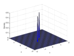
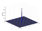
Figure 1. Here ρ0superscript𝜌0\rho^{0} and ρ1superscript𝜌1\rho^{1} are concentrated at (0,0)00(0,0), (0.4,0.4)0.40.4(0.4,0.4), i.e. ρ0=Ξ΄(0,0)superscript𝜌0subscript𝛿00\rho^{0}=\delta_{(0,0)}, ρ1=Ξ΄(0.4,0.4)superscript𝜌1subscript𝛿0.40.4\rho^{1}=\delta_{(0.4,0.4)}. The computed EMD-L1subscript𝐿1L_{1}, EMD-L2subscript𝐿2L_{2} is 0.79810.79810.7981, 0.62320.62320.6232
Refer to caption
(a) ρ0superscript𝜌0\rho^{0}.
Refer to caption
(b) ρ1superscript𝜌1\rho^{1}.
Figure 2. Here ρ0superscript𝜌0\rho^{0} is concentrated at (0,0)00(0,0), ρ1superscript𝜌1\rho^{1} is concentrated at two positions, (0.4,0.4)0.40.4(0.4,0.4) and (βˆ’0.4,βˆ’0.4)0.40.4(-0.4,-0.4), i.e. ρ0=Ξ΄(0,0)superscript𝜌0subscript𝛿00\rho^{0}=\delta_{(0,0)}, ρ1=12​(Ξ΄(0.4,0.4)+Ξ΄(βˆ’0.4,βˆ’0.4))superscript𝜌112subscript𝛿0.40.4subscript𝛿0.40.4\rho^{1}=\frac{1}{2}(\delta_{(0.4,0.4)}+\delta_{(-0.4,-0.4)}). The computed EMD-L1subscript𝐿1L_{1}, EMD-L2subscript𝐿2L_{2} is 0.80160.80160.8016, 0.62320.62320.6232.
Refer to caption
(a) ρ0superscript𝜌0\rho^{0}.
Refer to caption
(b) ρ1superscript𝜌1\rho^{1}.
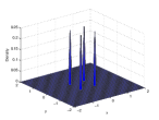
Figure 3. Here ρ0superscript𝜌0\rho^{0} is concentrated at (0,0)00(0,0), ρ1superscript𝜌1\rho^{1} is concentrated at four positions, (0.4,0.4)0.40.4(0.4,0.4), (0.4,βˆ’0.4)0.40.4(0.4,-0.4), (βˆ’0.4,0.4)0.40.4(-0.4,0.4), (βˆ’0.4,βˆ’0.4)0.40.4(-0.4,-0.4), i.e. ρ0=Ξ΄(0,0)superscript𝜌0subscript𝛿00\rho^{0}=\delta_{(0,0)}, ρ1=14​(Ξ΄(0.4,0.4)+Ξ΄(0.4,βˆ’0.4)+Ξ΄(βˆ’0.4,0.4)+Ξ΄(βˆ’0.4,βˆ’0.4))superscript𝜌114subscript𝛿0.40.4subscript𝛿0.40.4subscript𝛿0.40.4subscript𝛿0.40.4\rho^{1}=\frac{1}{4}(\delta_{(0.4,0.4)}+\delta_{(0.4,-0.4)}+\delta_{(-0.4,0.4)}+\delta_{(-0.4,-0.4)}). The computed EMD-L1subscript𝐿1L_{1}, EMD-L2subscript𝐿2L_{2} is 0.80020.80020.8002, 0.58820.58820.5882.
Refer to caption
(a) ρ0superscript𝜌0\rho^{0}.
Refer to caption
(b) ρ1superscript𝜌1\rho^{1}.
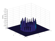
Figure 4. Here ρ0superscript𝜌0\rho^{0} is concentrated at (0,0)00(0,0), ρ1superscript𝜌1\rho^{1} is a measure supported on a circle, i.e. ρ0=Ξ΄(0,0)superscript𝜌0subscript𝛿00\rho^{0}=\delta_{(0,0)}, ρ1=1K​(ex2+y2Οƒβˆ’(x2+y2)2Οƒ)superscript𝜌11𝐾superscript𝑒superscriptπ‘₯2superscript𝑦2𝜎superscriptsuperscriptπ‘₯2superscript𝑦22𝜎\rho^{1}=\frac{1}{K}\big{(}e^{\frac{x^{2}+y^{2}}{\sigma}-\frac{(x^{2}+y^{2})^{2}}{\sigma}}\big{)}, where K𝐾K is a normalized constants and Οƒ=10βˆ’3𝜎superscript103\sigma=10^{-3}. The computed EMD-L1subscript𝐿1L_{1}, EMD-L2subscript𝐿2L_{2} is 0.87940.87940.8794, 0.69430.69430.6943.
Refer to caption
(a) ρ0superscript𝜌0\rho^{0}.
Refer to caption
(b) ρ1superscript𝜌1\rho^{1}.
Figure 5. Here ρ0=1K1​eβˆ’x2+y2βˆ’|x|βˆ’|y|Οƒsuperscript𝜌01subscript𝐾1superscript𝑒superscriptπ‘₯2superscript𝑦2π‘₯π‘¦πœŽ\rho^{0}=\frac{1}{K_{1}}e^{-\frac{x^{2}+y^{2}-|x|-|y|}{\sigma}}, ρ1=1K2​(ex2+y2Οƒβˆ’(x2+y2)2Οƒ)superscript𝜌11subscript𝐾2superscript𝑒superscriptπ‘₯2superscript𝑦2𝜎superscriptsuperscriptπ‘₯2superscript𝑦22𝜎\rho^{1}=\frac{1}{K_{2}}\big{(}e^{\frac{x^{2}+y^{2}}{\sigma}-\frac{(x^{2}+y^{2})^{2}}{\sigma}}\big{)}, where K1subscript𝐾1K_{1}, K2subscript𝐾2K_{2} are normalized constants and Οƒ=0.2𝜎0.2\sigma=0.2. The computed EMD-L1subscript𝐿1L_{1}, EMD-L2subscript𝐿2L_{2} is 0.17780.17780.1778, 0.12590.12590.1259.

Table 1, 2 reports the time under different grids for computing EMD-L1subscript𝐿1L_{1}, EMD-L2subscript𝐿2L_{2} in Figure 1, 2, 3. The implementation is done in MATLAB 201620162016, on a 2.40 GHZ Intel Xeon processor with 4GB RAM.

Example 1:
Grids number (N) Time (s) Iteration Relative Error 100100100 0.0411 58 0.2071 400400400 0.4015 167 0.1495 160016001600 4.78 524 0.1021 640064006400 64.81 1802 0.0607

Example 2:
Grids number (N) Time (s) Iteration Relative Error 100100100 0.089 133 0.2072 400400400 1.44 597 0.1497 160016001600 8.41 901 0.1014 640064006400 118.8 3001 0.0596

Example 3:
Grids number (N) Time (s) Iteration Relative Error 100100100 0.1334 210 0.0641 400400400 1.644 689 0.0536 160016001600 12.27 1347 0.0386 640064006400 130.37 3590 0.0199


Table 1. We compute EMD-L2subscript𝐿2L_{2} for Figure 1, 2, 3. Time is in seconds. The relative error is defined by |β€–mβ€–βˆ’0.4​2|0.4​2normπ‘š0.420.42\frac{|\|m\|-0.4\sqrt{2}|}{0.4\sqrt{2}}, where mπ‘šm is the computed minimizer of (3) and 0.4​20.420.4\sqrt{2} is the analytical solution of EMD-L2subscript𝐿2L_{2} (Euclidean distance between (0.4,0.4)0.40.4(0.4,0.4), (0,0)00(0,0)).

Example 1:
Grids number (N) Time (s) Iteration Relative Error 100100100 0.0310.0310.031 198198198 2.0Γ—10βˆ’32.0superscript1032.0\times 10^{-3} 400400400 0.1970.1970.197 356356356 7.5Γ—10βˆ’47.5superscript1047.5\times 10^{-4} 160016001600 1.6691.6691.669 786786786 2.7Γ—10βˆ’42.7superscript1042.7\times 10^{-4} 640064006400 25.178 305730573057 9.1Γ—10βˆ’59.1superscript1059.1\times 10^{-5}

Example 2:

Grids number (N) Time (s) Iteration Relative Error
100100100 0.047 156 1.0Γ—10βˆ’31.0superscript1031.0\times 10^{-3}
400400400 0.204 347 3.8Γ—10βˆ’43.8superscript1043.8\times 10^{-4}
160016001600 1.814 850 1.3Γ—10βˆ’41.3superscript1041.3\times 10^{-4}
640064006400 28.53 3483 4.6Γ—10βˆ’54.6superscript1054.6\times 10^{-5}

Example 3:

Grids number (N) Time (s) Iteration Relative Error
100100100 0.039 142 7.5Γ—10βˆ’47.5superscript1047.5\times 10^{-4}
400400400 0.171 261 2.6Γ—10βˆ’42.6superscript1042.6\times 10^{-4}
160016001600 1.678 803 8.9Γ—10βˆ’58.9superscript1058.9\times 10^{-5}
640064006400 31.13 3792 2.9Γ—10βˆ’52.9superscript1052.9\times 10^{-5}
Table 2. We compute EMD-L1subscript𝐿1L_{1} with Ο΅=0.01italic-Ο΅0.01\epsilon=0.01 for Figure 1, 2, 3. Here the stopping criteria is 1Nβ€‹βˆ‘i=1N|divG​(mik)+pi1βˆ’pi0|≀10βˆ’91𝑁superscriptsubscript𝑖1𝑁subscriptdiv𝐺subscriptsuperscriptπ‘šπ‘˜π‘–superscriptsubscript𝑝𝑖1superscriptsubscript𝑝𝑖0superscript109\frac{1}{N}\sum_{i=1}^{N}|\textrm{div}_{G}(m^{k}_{i})+p_{i}^{1}-p_{i}^{0}|\leq 10^{-9}. The relative error is defined by β€–mΟ΅β€–1+ϡ​‖mΟ΅β€–22βˆ’0.80.8subscriptnormsuperscriptπ‘šitalic-Ο΅1italic-Ο΅subscriptsuperscriptnormsuperscriptπ‘šitalic-Ο΅220.80.8\frac{\|m^{\epsilon}\|_{1}+\epsilon\|m^{\epsilon}\|^{2}_{2}-0.8}{0.8}, where mΟ΅superscriptπ‘šitalic-Ο΅m^{\epsilon} is the computed minimizer of (7) and 0.80.80.8 is the analytical solution of EMD-L1subscript𝐿1L_{1} (Manhattan distance between (0.4,0.4)0.40.4(0.4,0.4), (0,0)00(0,0)).

We observe that the number of iterations is roughly O​(N)𝑂𝑁O(N) (sometimes less). So we claim that the complexity of our algorithm is at most O​(N2)𝑂superscript𝑁2O(N^{2}), which roughly matches the result of the computation time in table 1 and 2.

Grids number (N) Time (s) EMD-L1subscript𝐿1L_{1} Time (s) in EMD-L2subscript𝐿2L_{2}
100100100 0.0162 0.1362
400400400 0.07529 1.645
160016001600 0.90 12.265
640064006400 22.38 130.37
Table 3. For Figure 3, we compare the computation time for EMD-L1subscript𝐿1L_{1} and EMD-L2subscript𝐿2L_{2}. Here we use the same stopping criteria: 1Nβ€‹βˆ‘i=1N|divG​(mik)+pi1βˆ’pi0|≀10βˆ’51𝑁superscriptsubscript𝑖1𝑁subscriptdiv𝐺subscriptsuperscriptπ‘šπ‘˜π‘–superscriptsubscript𝑝𝑖1superscriptsubscript𝑝𝑖0superscript105\frac{1}{N}\sum_{i=1}^{N}|\textrm{div}_{G}(m^{k}_{i})+p_{i}^{1}-p_{i}^{0}|\leq 10^{-5}.

We also observe that we get approximately 101010 times faster speed for EMD-L1subscript𝐿1L_{1} than EMD-L2subscript𝐿2L_{2} in table 3. This is expected, since it is expensive to compute square roots for the Euclidean ground metric.
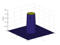
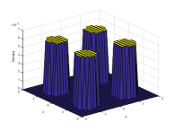
Refer to caption
(a) ρ0superscript𝜌0\rho^{0}.
Refer to caption
(b) ρ1superscript𝜌1\rho^{1}.
Refer to caption
(c) Manhattan distance.
Refer to caption
(d) Euclidean distance.
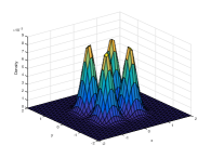
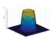
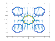
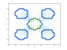
Figure 6. Comparison of minimizers m​(x)π‘šπ‘₯m(x) for EMD-L1subscript𝐿1L_{1} and EMD-L2subscript𝐿2L_{2}. Here the initial measure is a uniform measure supported on a disk while the terminal measure is a uniform measure supported on four disjoint disks.

It is also worth mentioning that the quadratic perturbation in modified problem (7) is necessary. We design the following two numerical results to demonstrate this.

  • (i)

    In table 4, we show that if we set Ο΅=0italic-Ο΅0\epsilon=0 in (7), the relative error can be enlarged if the total number of grids N𝑁N increases;

  • (ii)

    In table 5, we demonstrate that the minimizer of perturbed problem (7) approximates one particular minimizer of (3) when Ο΅italic-Ο΅\epsilon approaches 00.

Grids number N𝑁N Relative error
400 5.1Γ—10βˆ’55.1superscript1055.1\times 10^{-5}
1600 6.7Γ—10βˆ’56.7superscript1056.7\times 10^{-5}
6400 5.3Γ—10βˆ’45.3superscript1045.3\times 10^{-4}
Table 4. We compute EMD-L1subscript𝐿1L_{1} in Figure 3 with Ο΅=0italic-Ο΅0\epsilon=0 and different meshes. The terminal condition is 1Nβ€‹βˆ‘i=1N|divG​(mik)+pi1βˆ’pi0|≀10βˆ’61𝑁superscriptsubscript𝑖1𝑁subscriptdiv𝐺subscriptsuperscriptπ‘šπ‘˜π‘–superscriptsubscript𝑝𝑖1superscriptsubscript𝑝𝑖0superscript106\frac{1}{N}\sum_{i=1}^{N}|\textrm{div}_{G}(m^{k}_{i})+p_{i}^{1}-p_{i}^{0}|\leq 10^{-6}. The relative error is computed by |β€–m0β€–1βˆ’0.8|0.8subscriptnormsuperscriptπ‘š010.80.8\frac{|\|m^{0}\|_{1}-0.8|}{0.8}, where m0superscriptπ‘š0m^{0} is the computed minimizer of (7).
Ο΅italic-Ο΅\epsilon Relative error
0.10.10.1 9.1Γ—10βˆ’49.1superscript1049.1\times 10^{-4}
0.010.010.01 9.4Γ—10βˆ’59.4superscript1059.4\times 10^{-5}
0.0010.0010.001 1.6Γ—10βˆ’51.6superscript1051.6\times 10^{-5}
0.00010.00010.0001 6.0Γ—10βˆ’66.0superscript1066.0\times 10^{-6}
Table 5. We compute EMD-L1subscript𝐿1L_{1} in Figure 3 with a fixed mesh and different values of Ο΅italic-Ο΅\epsilon. The number of grid points is N=1600𝑁1600N=1600 and the terminal condition is 1Nβ€‹βˆ‘i=1N|divG​(mik)+pi1βˆ’pi0|≀10βˆ’61𝑁superscriptsubscript𝑖1𝑁subscriptdiv𝐺subscriptsuperscriptπ‘šπ‘˜π‘–superscriptsubscript𝑝𝑖1superscriptsubscript𝑝𝑖0superscript106\frac{1}{N}\sum_{i=1}^{N}|\textrm{div}_{G}(m^{k}_{i})+p_{i}^{1}-p_{i}^{0}|\leq 10^{-6} . The relative error is computed by |β€–mΟ΅β€–1+Ο΅2​‖mΟ΅β€–22βˆ’0.8|0.8subscriptnormsuperscriptπ‘šitalic-Ο΅1italic-Ο΅2superscriptsubscriptnormsuperscriptπ‘šitalic-Ο΅220.80.8\frac{|\|m^{\epsilon}\|_{1}+\frac{\epsilon}{2}\|m^{\epsilon}\|_{2}^{2}-0.8|}{0.8}, where mΟ΅superscriptπ‘šitalic-Ο΅m^{\epsilon} is the computed minimizer of (7).

5. Conclusions

To summarize, we applied a primal-dual algorithm to solve EMD with the L1subscript𝐿1L_{1}, L2subscript𝐿2L_{2} ground metric. The algorithm inherits both key ideas in optimal transport theory and homogenous degree one regularized problems. Compared to current methods, our algorithm has following advantages:

  • β€’

    First, it leverages the structure of optimal transport, which transfers EMD into a L1subscript𝐿1L_{1}-type minimization. The new minimization contains only N𝑁N variables, which is much less than the original N2superscript𝑁2N^{2} linear programming problem;

  • β€’

    Second, it uses simple exact formulas at each iteration (including the shrink operator) and converges to a minimizer.

  • β€’

    Third, it will be very easy to parallelize and thus speed up the algorithm considerably.

In addition, we consider a novel perturbed minimization

infm{βˆ«Ξ©β€–m​(x)​‖+Ο΅2‖​mβˆ₯22​d​x:βˆ‡β‹…m​(x)+ρ1​(x)βˆ’Ο0​(x)=0},subscriptinfimumπ‘šconditional-setsubscriptΞ©:evaluated-atπ‘šπ‘₯normitalic-Ο΅2π‘š22𝑑π‘₯β‹…βˆ‡π‘šπ‘₯superscript𝜌1π‘₯superscript𝜌0π‘₯0\inf_{m}\{\int_{\Omega}\|m(x)\|+\frac{\epsilon}{2}\|m\|_{2}^{2}dx~{}:~{}\nabla\cdot m(x)+\rho^{1}(x)-\rho^{0}(x)=0\}\ , (11)

to approximate EMD problem. Here βˆ₯β‹…βˆ₯\|\cdot\| can be either the 1-norm or the 2-norm. In future work, we will study several theoretical properties of (11), especially the relation between mΟ΅superscriptπ‘šitalic-Ο΅m^{\epsilon} and mπ‘šm when Ο΅italic-Ο΅\epsilon goes to 00.

References

  • [1] Luigi Ambrosio, Nicola Gigli, and Giuseppe SavarΓ©. Gradient flows: in metric spaces and in the space of probability measures. Springer Science & Business Media, 2006.
  • [2] M. Beckmann. A continuous model of transportation, Econometrica 20, 643 660, 1952.
  • [3] Jean-David Benamou and Yann Brenier. A computational fluid mechanics solution to the Monge-Kantorovich mass transfer problem. Numerische Mathematik 84(3): 375–393, 2000.
  • [4] Jean-David Benamou and Guillaume Carlier. Augmented Lagrangian methods for transport optimization, mean field games and degenerate elliptic equations. Journal of Optimization Theory and Applications, 167(1): 1–26, 2015.
  • [5] Jean-David Benamou, Guillaume Carlier and RomΓ©o Hatchi. A numerical solution to Monge’s problem with a Finsler distance as cost. M2AN, 2016.
  • [6] L.M. Brice o-Arias, D. Kalise and F.J. Silva. Proximal methods for stationary Mean Field Games with local couplings. arXiv:1608.07701, 2016.
  • [7] Antonin Chambolle and Thomas Pock. A first-order primal-dual algorithm for convex problems with applications to imaging. Journal of Mathematical Imaging and Vision, 120–145, 2011.
  • [8] B. Dacorogna and J. Moser. On a partial differential equation involving the Jacobian determinant. Annales de l’IHP Analyse non linΓ©aire, 7(1), 1–26, 1990.
  • [9] Lawrence Evans and Wilfrid Gangbo. Differential equations methods for the Monge-Kantorovich mass transfer problem. Memoirs of AMS, no 653, vol. 137, 1999.
  • [10] Mikhail Feldman and Robert McCann. Monge s transport problem on a Riemannian manifold. Transactions of the American Mathematical Society, 354 (4): 1667–1697, 2002.
  • [11] Tom Goldstein and Stanley Osher. The split Bregman method for L1-regularized problems. SIAM journal on imaging sciences, 2(2): 323-343, 2009.
  • [12] J. Gudmundsson, O. Klein, C. Knauer, and M. Small. Manhattan Networks and Algorithmic Applications for the Earth Movers Distance. In EWCG, 2007.
  • [13] E. Levina and P. Bickel. The earth mover’s distance is the Mallows distance: some insights from statistics Computer Vision, 2001. ICCV 2001. Proceedings. Eighth IEEE International Conference on (2):251–256, 2001.
  • [14] Wuchen Li. A study of stochastic differential equations and Fokker-Planck equations with applications. PhD thesis, 2016. Georgia Institute of Technology.
  • [15] H. Ling and K. Okada. An Efficient Earth Mover s Distance Algorithm for Robust Histogram Comparison. PAMI, 2007.
  • [16] L. MΓ©tivier, R. Brossier, Q. MΓ©rigot, E. Oudet and J. Virieux. Measuring the misfit between seismograms using an optimal transport distance: application to full waveform inversion Geophysical Journal International, (205) 1: 345–377, 2016.
  • [17] Ofir Pele and Michael Werman. Fast and robust earth mover’s distances. 2009 IEEE 12th International Conference on Computer Vision, 460–467, 2009.
  • [18] Thomas Pock and Antonin Chambolle. Diagonal preconditioning for first order primal-dual algorithms in convex optimization, 2011 International Conference on Computer Vision, 1762–1769, IEEE.
  • [19] Yossi Rubner, Carlo Tomasi and Leonidas Guibas. A metric for distributions with applications to image databases. Computer Vision, 1998. Sixth International Conference on, 59–66, IEEE, 1998.
  • [20] Yossi Rubner, Carlo Tomasi and Leonidas Guibas. The earth mover’s distance as a metric for image retrieval. International journal of computer vision, 40(2): 99–121, 2000.
  • [21] Leonid Rudin, Stanley Osher and Emad Fatemi. Nonlinear total variation based noise removal algorithms. Physica D: Nonlinear Phenomena, (60)1: 259-268, 1992.
  • [22] Filippo Santambrogio. Absolute continuity and summability of transport densities: simpler proofs and new estimates. Calculus of Variations and Partial Differential Equations, 36 (3): 343–354, 2009,
  • [23] Sameer Shirdhonkar and David Jacobs. Approximate earth mover s distance in linear time. Computer Vision and Pattern Recognition IEEE conference, 2008.
  • [24] Gilbert Strang. L1subscript𝐿1L_{1} and L∞subscript𝐿L_{\infty} approximation of vector fields in the plane. North-Holland Mathematics Studies, 81, 273–288, 1983.
  • [25] Justin Solomon, Raif Rustamov, Leonidas Guibas and Adrian Butscher. Earth mover’s distances on discrete surfaces. ACM Transactions on Graphics (TOG), 33(4), 2014.
  • [26] CΓ©dric Villani. Topics in optimal transportation. NumberΒ 58. American Mathematical Soc., 2003.
  • [27] Wotao Yin, Stanley Osher, Donald Goldfarb and Jerome Darbon. Bregman iterative algorithms for β„“1subscriptβ„“1\ell_{1}-minimization with applications to compressed sensing, SIAM Journal on Imaging sciences, 1(1): 143–168, 2008.