Large Margin Nearest Neighbor Classification using
Curved Mahalanobis Distances††thanks: A preliminary work appeared at IEEE International Conference on Image Processing (ICIP) 2016 [16].
Abstract
We consider the supervised classification problem of machine learning in Cayley-Klein projective geometries: We show how to learn a curved Mahalanobis metric distance corresponding to either the hyperbolic geometry or the elliptic geometry using the Large Margin Nearest Neighbor (LMNN) framework. We report on our experimental results, and further consider the case of learning a mixed curved Mahalanobis distance. Besides, we show that the Cayley-Klein Voronoi diagrams are affine, and can be built from an equivalent (clipped) power diagrams, and that Cayley-Klein balls have Mahalanobis shapes with displaced centers.
Keywords: classification; metric learning; Cayley-Klein metrics; LMNN; Voronoi diagrams.
1 Introduction
1.1 Metric learning
The Mahalanobis distance between point and of is defined for a symmetric positive definite matrix by:
| (1) |
It is a metric distance that satisfies the three metric axioms: indiscernibility ( iff. ), symmetry (), and triangle inequality (). The Mahalanobis distance generalizes the Euclidean distance by choosing , the identity matrix: . Given a finite point set , matrix is often chosen as the precision matrix where is the covariance matrix of :
| (2) | |||||
| (3) |
is the center of mass of (called sample mean in Statistics).
In machine learning, given a labeled point set with denoting the label of , the classification task consists in building a classifier to tag newly unlabelled points as . The classification task is binary when , otherwise it is said multi-task. A simple but powerful classifier consists in retrieving the nearest neighbor(s) of an unlabeled query point , and to associate to the dominant label of its neighbor(s). This rule yields the so-called -Nearest Neighbor classifier (or -NN for short). The -NN rule depends on the chosen distance between elements of . When the distance is parametric like the Mahalanobis distance, one has to learn the appropriate distance parameter (eg., matrix for the Mahalanobis distance). This hot topic of machine learning bears the name metric learning. Weinberger et al. [26] proposed an efficient method to learn a Mahalanobis distance: The Large Margin Nearest Neighbor (LMNN) algorithm. The LMNN algorithm was further extended to elliptic Cayley-Klein geometries in [4]. In this work, we further extend the LMNN framework in hyperbolic Cayley-Klein geometries, and also consider mixed hyperbolic/elliptic Cayley-Klein distances.
1.2 Contributions and outline
We summarize our key contributions as follows:
-
•
We extend the LMNN to hyperbolic Cayley-Klein geometries (§ 4.3),
-
•
We introduce a linearly mixed Cayley-Klein distance and investigate its experimental performance (§ 5.2),
-
•
We show that Cayley-Klein Voronoi diagrams are affine and equivalent to power diagrams (§ 3.1), and
-
•
We prove that Cayley-Klein balls have Mahalanobis shapes with displaced centers (§ 3.2).
The paper is organized as follows: Section 2 concisely introduces the basic notions of Cayley-Klein geometries and present formula for the elliptic/hyperbolic Cayley-Klein distances. Those elliptic/hyperbolic Cayley-Klein distances are reinterpreted as curved Mahalanobis distances in Section 2.4. Section 3 studies some facts useful for computational geometry [10]: First, we show that the Cayley-Klein bisector is a (clipped) hyperplane, and that the Cayley-Klein Voronoi diagrams can be built from equivalent (clipped) power diagrams (Section 3.1). Second, we notice that Cayley-Klein balls have Mahalanobis shapes with displaced centers (Section 3.2). Section 4 introduces the LMNN framework: First, we review LMNN for learning a squared Mahalanobis distance in § 4.1. Then we report the extension of Bi et al. [4] to elliptic Cayley-Klein geometries, and describe our novel extension to hyperbolic Cayley-Klein geometries in § 4.3. Experimental results are presented in Section 5, and a mixed Cayley-Klein distance is considered in § 5.2 that further improve experimentally classification performance. Fast nearest neighbor queries in Cayley-Klein geometries are briefly touched upon in § 5.1. Finally, Section 6 concludes this work and hints at further perspectives of the role of Cayley-Klein distances in machine learning.
2 Cayley-Klein geometry
The real projective space [22] can be understood as the set of lines passing through the origin of the vector space . Projective spaces is different from spherical geometry because antipodal points of the unit sphere are identified (they yield the same line passing through the origin). Let denote the real projective space with the equivalence class relation : for . A point in is mapped to a point using homogeneous coordinates by adding an extra coordinate . Conversely, a projective point is dehomogeneized by “perspective division” provided that . The projective points at infinity have the coordinate . Thus the projective space is a compactification of the Euclidean space. The non-infinite points of the projective space is often visualized in as the points lying on the hyperplane passing through the -th coordinate (with each point on defining a line passing through the origin of ). In projective geometry, two distinct lines always intersect in exactly one point, and a bundle of Euclidean parallel lines intersect at the same projective point at infinity.
In projective geometry [22], the cross-ratio (Figure 1) of four collinear points on a line is defined by:
| (4) |
The cross-ratio is a measure that is invariant by projectivities [22] (see Figure 1 (a)), also called collineations or homographies. The cross-ratio enjoys the following key properties:
-
•
,
-
•
,
-
•
when is collinear with .
 |
 |
| (a) | (b) |
A gentle introduction to projective geometry and Cayley-Klein geometries can be found in [22, 24, 25]. We also refer the reader to a more advanced textbook [20] handling invariance and isometries, and to the historical seminal paper [7] of Cayley (1859).
2.1 Cayley-Klein distances from cross-ratio measures
A Cayley-Klein geometry is a triple , where:
-
1.
is a fundamental conic,
-
2.
is a constant unit for measuring distances, and
-
3.
is constant unit for measuring angles.
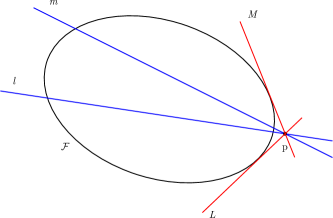
The distance in Cayley-Klein geometries (see Figure 2) is defined by:
| (5) |
where and are the intersection points of line with the fundamental conic . Historically, the fundamental conic was called the “absolute” [7]. The logarithm function denotes the principal value of the complex logarithm. That is, since complex logarithm values are defined up to modulo , we define the principal value of the complex logarithm as the unique value with imaginary part lying in the range .
 |
 |
| (a) distance measurement | (b) angle measurement |
Similarly, the angle in Cayley-Klein geometries (see Figure 2) is measured as follows:
| (6) |
where and are tangent lines to the fundamental conic passing through the intersection point of line and line (see Figure 2). This formula generalizes the Laguerre formula that calculates the acute angle between two distinct real lines [22].
The Cayley-Klein geometries can further be extended to Hilbert projective geometries [9] by replacing the conic object with a bounded convex subset of . Interestingly, the convex objects delimiting the Hilbert geometry domain do not need to be strictly convex [8].
The properties of Cayley-Klein distances are:
-
•
Law of the indiscernibles: iff. ,
-
•
Signed distances : , and
-
•
When are collinear, . That is, shortest-path geodesics111Cayley-Klein geometries can also be studied from the viewpoint of Riemannian geometry. in Cayley-Klein geometries are straight lines (clipped within the conic domain ).
Notice that the logarithm of Cayley-Klein measurement formula is transferring multiplicative properties of the cross-ratio to additive properties of Cayley-Klein distances: For example, it follows from the cross-ratio identity for collinear that .
2.2 Dual conics and taxonomy of Cayley-Klein geometries
In projective geometry, points and lines are dual concepts, and theorems on points can be translated equivalently to theorems on lines. For example, Pascal’s theorem is dual to Brianchon’s theorem [22].
A conic object can be described as the convex hull of its extreme points (points lying on its border), or equivalently as the intersection of all half-spaces tangent at its border and fully containing the conic. This is similar to the dual -representation and -representation of finite convex polytopes [13] (’H’ standing for Halfspaces, and ’V’ for Vertex). This point/line duality yields a dual parameterizations of the fundamental conic by two matrices, where is the adjoint matrix (transpose of its cofactor matrix). Observe that the adjoint matrix can be computed even when is not invertible ().
To a symmetric positive semi-definite matrix -dimensional , we associate a homogeneous polynomial called the quadratic form . The primal conic is thus described as the set of border points using matrix , and the dual conic as the set of tangent hyperplanes using the dual adjoint matrix .
The signature of matrix is a triple counting the signs of the eigenvalues (in ) of its eigendecomposition, where denotes the number of negative eigenvalue(s), the number of null eigenvalue(s), and the number of positive eigenvalue(s) (with ). For example, a symmetric positive-definite matrix has signature , while a semi-definite rank-deficient matrix of rank has signature .
Table 1 displays the seven types of planar Cayley-Klein geometries (induced by a pair of dual conic matrices ). All degenerate cases can be obtained as the limit of non-degenerate cases, see [22]. Another way to classify the Cayley-Klein geometries is to consider the type of measurements for distances and angles. Each type of measurement is of three kinds [22]: elliptic or hyperbolic for non-degenerate geometries or parabolic for degenerate cases. Using this classification, we obtain nine combinations for the planar Cayley-Klein geometries.
| Type | Conic in | ||
|---|---|---|---|
| Elliptic | non-degenerate complex conic | ||
| Hyperbolic | non-degenerate real conic | ||
| Dual Euclidean | Two complex lines with a real intersection point | ||
| Dual Pseudo-euclidean | Two real lines with a double real intersection point | ||
| Euclidean | Two complex points with a double real line passing through | ||
| Pseudo-euclidean | Two complex points with a double real line passing through | ||
| Galilean | Double real line with a real intersection point |
Traditionally, hyperbolic geometry [2] considers objects inside the unit ball in the Beltrami-Klein model. In that case, the fundamental conic that is the unit ball. However, using Cayley-Klein geometry, complex-valued measures are also possible even when points/lines fall outside the fundamental conic. With the following choice and , we obtain [22] (Chapter 20):
-
•
A real measurement for angles when points lie inside the primal conic,
-
•
When both points and lie outside the conic, with denoting the line passing through them:
-
–
A real hyperbolic measure if does not intersect the conic,
-
–
A pure imaginary elliptical measure if does not intersect the conic,
-
–
-
•
A complex measure () if one point is inside, and the other outside the conic.
Therefore it may be convenient to use in general the module of Cayley-Klein measures to handle all those possible situations.
In higher dimensions [14, 22], Cayley-Klein geometries unify common space geometries (euclidean, elliptical, and hyperbolic) with other space-time geometries (Minkowskian, Galilean, de Sitter, etc.) In the remainder, we consider the non-degenerate hyperbolic Cayley-Klein geometry (signature , a real conic) and the non-degenerate elliptic Cayley-Klein geometry (signature , a complex conic).
2.3 Bilinear form and formula for the hyperbolic/elliptic Cayley-Klein distances
For getting real-value Cayley-Klein distances, we choose the constants as follows (with denoting the curvature) :
-
•
Elliptic (): ,
-
•
Hyperbolic (): .
By introducing the bilinear form for a matrix S:
| (7) |
we get rid of the cross-ratio expression in distance/angle formula of Eq. 5 and Eq. 6 using [22]:
| (8) |
Thus, we end up with the following equivalent expressions for the elliptic/hyperbolic Cayley-Klein distances:
- Hyperbolic Cayley-Klein distance.
-
When (the hyperbolic domain), we have the following equivalent hyperbolic Cayley-Klein distances:
(9) (10) (11) where and .
- Elliptic Cayley-Klein distance.
-
When , we have the following equivalent elliptic Cayley-Klein distances:
(12) (13)
Since the elliptic/hyperbolic case is induced by the signature of matrix , we shall denote generically by the Cayley-Klein distance in either the elliptic or hyperbolic case.
Those elliptic/hyperbolic distances can be interpreted from projections [22, 18], as depicted in Figure 3.
 |
 |
| (a) gnomonic projection | (b) central projection |
| Euclidean inner product | Minkowski inner product |
| hemisphere model | hyperboloid model |
It is somehow surprising that we can derive metric structures from projective geometry. Arthur Cayley (1821-1895), a British mathematician, said “Projective geometry is all geometry”.
2.4 Cayley-Klein elliptic/hyperbolic distances: Curved Malahanobis distances
Bi et. al [4] rewrote the bilinear form as follows: Let
| (14) |
with a -dimensional matrix and so that:
| (15) |
Let (so that ) and so that:
| (16) |
Then the bilinear form can be rewritten as:
| (17) |
Furthermore, it is proved in [4] that:
| (18) |
Therefore the hyperbolic/elliptic Cayley-Klein distances can be interpreted as curved Mahalanobis distances (or -Mahalanobis distances). Indeed, we choose to term those hyperbolic/elliptic Cayley-Klein distances “curved Mahalanobis distances” to constrast with the fact that (squared) Mahalanobis distances are symmetric Bregman divergences that induce a (self-dual) flat geometry in information geometry [1].
Notice that when , we recover the canonical hyperbolic distance [17] in Cayley-Klein model:
| (19) |
defined inside the interior of a unit ball since we have:
| (20) |
3 Computational geometry in Cayley-Klein geometries
3.1 Cayley-Klein Voronoi diagrams
Define the bisector of points and as:
| (21) |
Then it comes that the bisector is a hyperplane (eventually clipped to the domain ) with equation:
| (22) | |||||
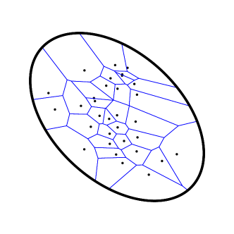
Figure 4 displays two examples of the bisectors of two points in planar hyperbolic Cayley-Klein geometry.
Thus the Cayley-Klein Voronoi diagram is an affine diagram. Therefore the Cayley-Klein Voronoi diagram can be computed as an equivalent (clipped) power diagram [15, 5, 17], using the following conversion formula:
| (23) | |||||
| (24) |
where is the equivalent ball of point .
More precisely, let denote the set of associated balls of . Then the Cayley-Klein Voronoi diagram of amounts to the intersection of the power Voronoi diagram of equivalent balls clipped to the domain :
| (25) |
Figure 5 and a short online video222https://www.youtube.com/watch?v=YHJLq3-RL58 illustrates the Cayley-Klein Voronoi diagrams.
3.2 Cayley-Klein balls have Mahalanobis shapes with displaced centers
A Cayley-Klein ball of center and radius is defined by:
| (26) |
The Cayley-Klein sphere has equation .
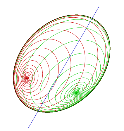
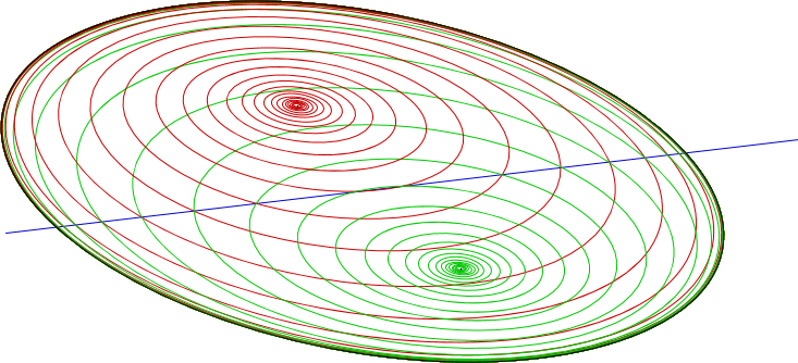
Figure 6 shows Cayley-Klein spheres in the elliptic case (red), and in the hyperbolic case (green) at different center positions (but for fixed elliptic and hyperbolic geometries). For comparison, the Mahalanobis spheres are displayed (blue): This drawing let us visualize the anisotropy of Cayley-Klein spheres that have shape depending on the center location, while Mahalanobis spheres have identical shapes everywhere (isotropy).
It can be noticed in Figure 6 that Cayley-Klein balls have Mahalanobis ball shapes with displaced centers. We shall give the corresponding conversion formula. Let
| (27) |
denote the equation of a Mahalanobis sphere of center , radius , and shape . Then a hyperbolic/elliptic sphere can be interpreted as a Mahalanobis sphere as follows:
- Hyperbolic Cayley-Klein sphere case:
-
- Elliptic Cayley-Klein sphere case:
-
Furthermore, by using the Cholesky decomposition of , a Mahalanobis sphere can be interpreted as an ordinary Euclidean sphere after performing an affine transformation .
| (28) | |||||
| (29) | |||||
| (30) | |||||
| (31) |

4 Learning curved Mahalanobis metrics
Supervised learning techniques rely on labelled information, or at least on side information based on similarities/dissimilarities. In the technique called Mahalanobis Metric for Clustering (MMC) [27], Xing and al. use pairwise information to learn a global Mahalanobis metric. Given two sets and of input describing respectively the pairs of points that are similar to each other (eg., share the same label) and the pairs which are dissimilar (eg., have different labels), Xing and al. [27] learn a matrix by gradient descent such that the total pairwise distance in in maximized, while keeping the total pairwise distance in constant. While good performances are experimentally obtained, this MMC method tends to cluster similar points together and may thus perform poorly in the case of multi-modal data. Furthermore, MMC requires two computationally costly projections at each gradient step: One projection on the cone of positive semi-definite matrices, and the other projection on the set of constraints.
LMNN [26] on the other hand is a projection-free metric learning method. LMNN learns a global Mahalanobis metric using triplet information: For each point, we take as input a set of target neighbors which should be brought close by the learned metric, while enforcing a unit margin with respect to points which are differently labelled. Contrary to MMC, LMNN handles well multi-modal data, but would optimally require oracle information of which points should be considered as targets of a given point. In practice, this is achieved by computing for each point the list of its nearest neighbors according to euclidean distance beforehand, but in specific applications the “point neighborhoods” can be gained using additional structural properties of the problems at hand.
While we consider in the remainder the LMNN framework, another more flexible approach in metric learning consists in learning local metrics, which allow to obtain a non-linear pseudo-metric while staying in a Mahalanobis framework333In Riemannian geometry, the distance is a geodesic length that can be interpreted as locally integrating Mahalanobis infinitesimal distances: for a metric tensor ., at the cost of greatly amplifying spatial complexity. Therefore, most works on the subject try to obtain a sparse encoding of such metrics. For example, in [12], Fetaya and Ullman learn one Mahalanobis metric per data point using only negative examples (eg., only information on dissimilarity), and obtain sparse metrics thanks to an equivalence with Support Vector Machines (SVMs). In [23], Shi et. al. sparsely combine low-rank (one-dimensional) local metrics into a global metric. For a comprehensive survey on local metric learning, we refer the reader to [21].
4.1 Large Margin Nearest Neighbors (LMNN)
Given a labeled input data-set of points of , the Large Margin Nearest Neighbors444http://www.cs.cornell.edu/~kilian/code/lmnn/lmnn.html (LMNN) [26] learns a Mahalanobis distance (ie., matrix ). Since the -NN classification does not change by taking any monotonically increasing function of the base distance (like its square), it is often more convenient mathematically to use the squared Mahalanobis distance that get rid of the square root. However, the squared Mahalanobis distance does not satisfy the triangle inequality. (It is a Bregman divergence [3, 15, 5].)
In LMNN, for each point, we take as input the set of target neighbors which should be brought close by the learned metric, while enforcing a unit margin with respect to points which have different labels.
To define the objective cost function [26] in LMNN, we consider two sets and , or target neighbors and impostors:
-
•
Distance of each point to its target neighbors shrink, :
(32) where denotes the neighbors of point .
-
•
Keep a distance margin of each point to its impostors, :
(33)
Using Cholesky decomposition , the LMNN cost function [26] is then defined as:
| (34) | |||||
| (35) | |||||
| (36) |
where and is a trade-off parameter for tuning target/impostor relative importance, and indicates that is a target neighbor of . We define if and only if and have same label, otherwise.
Thus the training of the Mahalanobis matrix is done by minimizing a linear combination of a pull function which brings points closer to their target neighbors with a push function that keeps the impostors away by penalizing the violation of the margin with a hinge loss.
The LMNN cost function is convex and piecewise linear [26]. Replacing the hinge loss by slack variables, we obtain a semidefinite program, which allows us to solve the minimization problem with standard solver packages.
Instead, Weinberger and Saul [26] propose a gradient descent where the set of impostors is re-computed every to iterations.
In our implementation, we optimize the cost function by gradient descent:
| (37) |
where is the learning rate, and:
| (38) |
with .
LMNN is a projection-free metric learning method that is quite easy to implement. There is no projection mechanism like for the Mahalanobis Metric for Clustering (MMC) [27] method.
We shall now consider extensions of the LMNN method to Cayley-Klein elliptic [4] and hyperbolic geometries.
4.2 Elliptic Cayley-Klein LMNN
Bi et al. [4] consider the extension of LMNN to the case of elliptic Cayley-Klein geometry. The cost function is defined as:
| (39) |
with
| (40) |
The gradient555There is minor error in the expression of in the original paper of Bi et al. [4], as was replaced by , which cannot be the distance gradient that must be symmetric with respect to and . with respect to lower triangular matrix is computed as:
| (41) |
with .
The gradient terms of Eq. 41 are calculated as follows:
| (42) | |||||
| (43) |
The elliptic LMNN loss is not convex, and thus the performance of the algorithm greatly depends on the chosen initialization for . We may initialize the elliptic CK-LMNN either by the sample mean of the point set , and either the precision matrix (inverse covariance matrix) of or the matrix obtained by Mahalanobis-LMNN. We then build initial matrix as follows:
| (44) |
Such a matrix is called a generalized Mahalanobis matrix in [4]. We term them curved Mahalanobis matrices.
Note that elliptic Cayley-Klein geometry are defined on the full domain , and furthermore the elliptic distance is bounded (by when ).
4.3 Hyperbolic Cayley-Klein LMNN
To ensure that the -dimensional matrix keeps the correct signature during the LMNN gradient descent, we decompose (with ) and perform a gradient descent on with the following gradient:
| (45) |
We initialize and so that as follows: Let (eg., by taking precision matrix of ), and then choose the diagonal matrix as:
| (46) |
with .
Let denote the domain at a given iteration induced by the bilinear form . It may happen that the point set since we do not know the optimal learning rate beforehand, and thus might have overshoot the domain. When this case happens, we reduce , otherwise when the point set is fully contained inside the real conic domain, we let .
Like in the elliptic case, we initialize the hyperbolic CK-LMNN either by calculating the sample mean of the point set , and either the precision matrix of or the matrix obtained by Mahalanobis-LMNN. We then build initial matrix as follows:
| (47) |
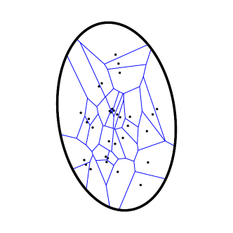
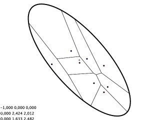
Figure 7 displays a hyperbolic Cayley-Klein Voronoi diagram for a set of generators (with labels displayed in blue/red), and the bichromatic Voronoi diagram in case of binary classification. Notice that the decision frontier of the nearest-neighbor classifier () is the union of Voronoi facets (in 2D, edges) supporting different label cells. A similar result holds for the Cayley-Klein -NN classifier: Its decision boundary is piecewise linear since the bisectors are (clipped) hyperplanes.
 |
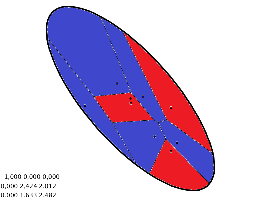 |
| (a) | (b) |
5 Experimental results
We report on our experimental results on some UCI data-sets.666https://archive.ics.uci.edu/ml/datasets.html Descriptions of those labelled data-sets are concisely summarized in Table 3.
| Data-set | # Data points | # Attributes | # Classes |
|---|---|---|---|
| Wine | 178 | 13 | 3 |
| Sonar | 208 | 60 | 2 |
| Vowel | 528 | 10 | 11 |
| Balance | 625 | 4 | 3 |
| Pima | 768 | 8 | 2 |
We performed nearest neighbor classification.
As in [4], we performed leave-one-out cross validation for the wine data-set, whereas for balance, pima and vowel data-sets, we trained the model on random subsets of size , testing it on the remaining data and repeating this procedure times.
| k | Data-set | elliptic | Hyperbolic | Mahalanobis |
|---|---|---|---|---|
| 1 | wine | 0.989 | 0.865 | 0.984 |
| vowel | 0.832 | 0.797 | 0.827 | |
| balance | 0.924 | 0.891 | 0.846 | |
| pima | 0.726 | 0.706 | 0.709 | |
| 3 | wine | 0.983 | 0.871 | 0.984 |
| vowel | 0.828 | 0.782 | 0.827 | |
| balance | 0.917 | 0.911 | 0.846 | |
| pima | 0.706 | 0.695 | 0.709 | |
| 5 | wine | 0.983 | 0.984 | |
| vowel | 0.826 | 0.805 | 0.827 | |
| balance | 0.907 | 0.895 | 0.846 | |
| pima | 0.714 | 0.712 | 0.709 | |
| 11 | wine | 0.994 | 0.983 | 0.984 |
| vowel | 0.839 | 0.767 | 0.827 | |
| balance | 0.874 | 0.897 | 0.846 | |
| pima | 0.713 | 0.698 | 0.709 |
We observe that the elliptic CK-LMNN performs quite better than the Mahalanobis LMNN and the hyperbolic CK-LMNN.
5.1 Spectral decomposition and proximity queries in Cayley-Klein geometry
To avoid to compute or for arbitrary matrix , we apply the matrix factorization (elliptic case , or hyperbolic case ) and perform coordinate changes so that it is enough to consider the canonical metric distances:
| (48) | |||||
| (49) |
Alternatively, consider the spectral decomposition of matrix obtained by eigenvalue decomposition (with diagonal matrix ), and let us write canonically:
| (50) |
where and is an orthogonal matrix (with ). The diagonal matrix has all positive values, with and so that is defined as the diagonal matrix obtained by taking element-wise the square root values of the matrix.
We rewrite the bilinear form into a canonical form by mapping the points to . Since , we can then find . When (elliptical case with ), we have . When (hyperbolic case with ), we have , with the canonical matrix form for hyperbolic Cayley-Klein spaces.
Notice that in the ordinary Mahalanobis case, instead of using the Cholesky decomposition, we may also use the matrix decomposition where is a unit lower triangular matrix (with diagonal elements all ), and is a diagonal matrix of positive elements. The mapping is then or since . Thus by transforming the input space into one of the canonical Euclidean/elliptical/hyperbolic spaces, we avoid to perform costly matrix multiplications required in the general bilinear form, and once the structure (say, a -NN decision boundary or a Voronoi diagram) has been recovered, we can map back to the original space (say, for classifying new observations using the original coordinate system).
Nearest neighbor proximity queries can then be answered using various spatial data-structures. For example, we may consider the Vantage Point Tree data-structures [28, 19].
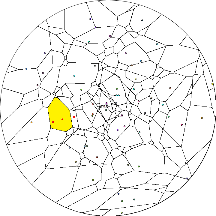
In small dimensions, we can compute the -order elliptic/hyperbolic Voronoi affine diagram, as depicted in Figure 8. The -order Voronoi diagram is affine since the bisectors are affine. Neighbor queries can then be reported efficiently in logarithmic time in 2D after preprocessing time, see [10] for further details.
5.2 Mixed curved Mahalanobis distance
We consider the mixed elliptic/hyperbolic Cayley-Klein distance:
| (51) |
Since the sum of (Riemannian) metric distances is a (Riemannian) metric distance, we deduce that is a (Riemannian) metric distance. However, this “blending” of positive with negative constant curvature (Riemannian) geometries does not yield a constant curvature (Riemannian) geometry. Indeed, although that the metric tensors blend locally, the Ordinary Differential Equation (ODE) characterizing the geodesics solves differently.
Notice that we mix a bounded distance (elliptic CK) with an unbounded distance (hyperbolic CK) via the hyperparameter that needs to be tuned. Table 5 shows the preliminary experimental results. Those results indicate better performance for the mixed model in most (but not all) cases. This should not be surprising as a smooth non-constant Riemannian manifold will better model data-sets than a constant-curvature manifold.
| Datasets | Mahalanobis | elliptic | Hyperbolic | Mixed | ||
|---|---|---|---|---|---|---|
| Wine | 0.993 | 0.984 | 0.893 | 0.986 | 0.741 | 0.259 |
| Sonar | 0.733 | 0.788 | 0.640 | 0.802 | 0.794 | 0.206 |
| Balance | 0.846 | 0.910 | 0.904 | 0.920 | 0.440 | 0.560 |
| Pima | 0.709 | 0.712 | 0.699 | 0.720 | 0.584 | 0.416 |
| Vowel | 0.827 | 0.825 | 0.816 | 0.841 | 0.407 | 0.593 |
6 Conclusion and perspectives
We considered Cayley-Klein geometries for super-vised classification purposes in machine learning. First, we studied some nice properties of the Voronoi diagrams and balls in Cayley-Klein geometries: We proved that the Cayley-Klein Voronoi diagram is affine, and reported formula to build it as an equivalent (clipped) power diagram. We then showed that Cayley-Klein balls have Mahalanobis shapes with displaced centers, and gave the explicit conversion formula. Second, we extended the LMNN framework to hyperbolic Cayley-Klein geometries that were not considered in [4], and proposed learning a mixed elliptic/hyperbolic distance that experimentally shows good improvement over constant-curvature Cayley-Klein geometries.
The fact that the Cayley-Klein bisectors are hyperplanes offers nice computational perspectives in machine learning and computational geometry. For example, it would be interesting to study Multi-Dimensional Scaling [11] or Support Vector Machines (SVMs) in Cayley-Klein geometries, or to mesh anisotropically [6] in Cayley-Klein geometries.
Supplemental information is available online at:
https://www.lix.polytechnique.fr/~nielsen/CayleyKlein/
References
- [1] S. Amari. Information Geometry and Its Applications. Applied Mathematical Sciences. Springer Japan, 2016.
- [2] James Anderson. Hyperbolic geometry. Springer Science & Business Media, 2006.
- [3] Arindam Banerjee, Srujana Merugu, Inderjit S Dhillon, and Joydeep Ghosh. Clustering with Bregman divergences. Journal of machine learning research, 6(Oct):1705–1749, 2005.
- [4] Yanhong Bi, Bin Fan, and Fuchao Wu. Beyond Mahalanobis metric: Cayley-Klein metric learning. In The IEEE Conference on Computer Vision and Pattern Recognition (CVPR), June 2015.
- [5] Jean-Daniel Boissonnat, Frank Nielsen, and Richard Nock. Bregman Voronoi diagrams. Discrete & Computational Geometry, 44(2):281–307, 2010.
- [6] Jean-Daniel Boissonnat, Camille Wormser, and Mariette Yvinec. Anisotropic Delaunay mesh generation. SIAM Journal on Computing, 44(2):467–512, 2015.
- [7] Arthur Cayley. A sixth memoir upon quantics. Philosophical Transactions of the Royal Society of London, 149:61–90, 1859.
- [8] Bruno Colbois, Constantin Vernicos, and Patrick Verovic. Hilbert geometry for convex polygonal domains. Journal of Geometry, 100(1):37–64, 2011.
- [9] Bruno Colbois and Patrick Verovic. Hilbert geometry for strictly convex domains. Geometriae Dedicata, 105(1):29–42, 2004.
- [10] Mark De Berg, Marc Van Kreveld, Mark Overmars, and Otfried Cheong Schwarzkopf. Computational geometry. Springer, 2000.
- [11] Jan Drösler. Foundations of multi-dimensional metric scaling in Cayley-Klein geometries. British Journal of Mathematical and Statistical Psychology, 32(2):185–211, 1979.
- [12] E. Fetaya and S. Ullman. Learning local invariant mahalanobis distances. International Conference on Machine Learning (ICML), 2015.
- [13] Branko Grünbaum. Convex Polytopes, volume 221. Springer Science & Business Media, 2013.
- [14] C. Gunn. Geometry, Kinematics, and Rigid Body Mechanics in Cayley-Klein Geometries. PhD thesis, Technische Universität Berlin, 2011.
- [15] Frank Nielsen, Jean-Daniel Boissonnat, and Richard Nock. On Bregman Voronoi diagrams. In Proceedings of the eighteenth annual ACM-SIAM symposium on Discrete algorithms, pages 746–755. Society for Industrial and Applied Mathematics, 2007.
- [16] Frank Nielsen, Boris Muzellec, and Richard Nock. Classification with mixtures of curved Mahalanobis metrics. In IEEE International Conference on Image Processing (ICIP), pages 241–245, Sept 2016.
- [17] Frank Nielsen and Richard Nock. Hyperbolic Voronoi diagrams made easy. In IEEE International Conference on Computational Science and Its Applications (ICCSA), pages 74–80, 2010.
- [18] Frank Nielsen and Richard Nock. Further results on the hyperbolic Voronoi diagrams. CoRR, abs/1410.1036, 2014.
- [19] Frank Nielsen, Paolo Piro, and Michel Barlaud. Bregman vantage point trees for efficient nearest neighbor queries. In IEEE International Conference on Multimedia and Expo, pages 878–881. 2009.
- [20] Arkadij L Onishchik and Rolf Sulanke. Projective and Cayley-Klein Geometries. Springer Science & Business Media, 2006.
- [21] D. Ramanan and S. Baker. Local distance functions: A taxonomy, new algorithms, and an evaluation. Pattern Analysis and Machine Intelligence, IEEE Transactions on, 33(4):794–806, April 2011.
- [22] Jürgen Richter-Gebert. Perspectives on Projective Geometry: A Guided Tour Through Real and Complex Geometry. Springer, 2011.
- [23] Yuan Shi, Aurélien Bellet, and Fei Sha. Sparse compositional metric learning. In Proceedings of the Twenty-Eighth AAAI Conference on Artificial Intelligence, pages 2078–2084, 2014.
- [24] Horst Struve and Rolf Struve. Projective spaces with Cayley-Klein metrics. Journal of Geometry, 81(1-2):155–167, 2004.
- [25] Horst Struve and Rolf Struve. Non-euclidean geometries: the Cayley-Klein approach. Journal of Geometry, 98(1-2):151–170, 2010.
- [26] Kilian Q. Weinberger, John Blitzer, and Lawrence K. Saul. Distance metric learning for large margin nearest neighbor classification. In In Advances in neural information processing systems (NIPS). MIT Press, 2006.
- [27] Eric P. Xing, Andrew Y. Ng, Michael I. Jordan, and Stuart Russell. Distance metric learning, with application to clustering with side-information. In Advances in neural information processing systems*15, pages 505–512. MIT Press, 2003.
- [28] Peter N. Yianilos. Data structures and algorithms for nearest neighbor search in general metric spaces. In Proceedings of the Fourth Annual ACM-SIAM Symposium on Discrete Algorithms, SODA ’93, pages 311–321, Philadelphia, PA, USA, 1993. Society for Industrial and Applied Mathematics.