On percolation critical probabilities and unimodular random graphs

Abstract

We investigate generalisations of the classical percolation critical probabilities ${p_{c}}$, ${p_{T}}$ and the critical probability ${\tilde{p}_{c}}$ defined by Duminil-Copin and Tassion [11] to bounded degree unimodular random graphs. We further examine Schramm’s conjecture in the case of unimodular random graphs: does ${p_{c}}(G_{n})$ converge to ${p_{c}}(G)$ if $G_{n}\to G$ in the local weak sense? Among our results are the following:

• ${p_{c}}={\tilde{p}_{c}}$ holds for bounded degree unimodular graphs. However, there are unimodular graphs with sub-exponential volume growth and ${p_{T}}<{p_{c}}$; i.e., the classical sharpness of phase transition does not hold.

• We give conditions which imply $\lim{p_{c}}(G_{n})={p_{c}}(\lim G_{n})$.

• There are sequences of unimodular graphs such that $G_{n}\to G$ but ${p_{c}}(G)>\lim{p_{c}}(G_{n})$ or ${p_{c}}(G)<\lim{p_{c}}(G_{n})<1$.

As a corollary to our positive results, we show that for any transitive graph with sub-exponential volume growth there is a sequence $\mathcal{T}_{n}$ of large girth bi-Lipschitz invariant subgraphs such that ${p_{c}}(\mathcal{T}_{n})\to 1$. It remains open whether this holds whenever the transitive graph has cost 1.

1 Introduction

1.1 Motivation and results

There are several definitions of the critical probability for percolation on the lattices $\mathbb{Z}^{d}$, which have turned out to be equivalent not only on $\mathbb{Z}^{d}$, but also in the more general context of arbitrary transitive graphs [28, 1, 16, 4, 11, 12]. One of our goals is to investigate the relationship between these different definitions when the graph $G$ is an ergodic unimodular random graph [9, 2], which is the natural extension of transitivity to the disordered setting. We examine the generalisations of ${p_{c}}=\sup\{p:\mathrm{\mathbb{P}}_{p}(\textrm{there is an infinite cluster})=0\}$, ${p_{T}}=\sup\left\{p:\mathrm{\mathbb{E}}_{p}(|\mathcal{C}_{o}|)<\infty\right\}$ and ${\tilde{p}_{c}}$, defined by Duminil-Copin and Tassion [11]. The last quantity was in fact designed to give a simple new proof of $p_{c}=p_{T}$ for transitive graphs, and to address the question of locality of critical percolation: whether the value of $p_{c}$ depends only on the local structure of the graph.

More precisely, Schramm’s “locality conjecture”, stated first explicitly in [8], says that ${p_{c}}(G_{n})\to{p_{c}}(G)$ holds whenever $G_{n}$ is a sequence of vertex-transitive infinite graphs such that $G_{n}$ converges locally to $G$ (i.e., for every radius $r$, the $r$-ball in $G_{n}$, for $n$ large enough, is isomorphic to the $r$-ball in $G$) and $\sup_{n}{p_{c}}(G_{n})<1$. Typically, however, the natural setting for such locality statements is not the class of transitive graphs, but the class of unimodular random graphs. Indeed, there are several interesting probabilistic quantities, most often related in some way to random walks, which have turned out to possess locality, mostly in the generality of unimodular random graphs: see [9, 23, 25, 10, 6, 17] for specific examples, and [30, Chapter 14] for a partial overview. Therefore, it is natural to investigate Schramm’s conjecture in the setup of unimodular random graphs and see what the proper notion of critical probability may be from the point of view of locality.

The conjecture has been proved for some special transitive graphs. Grimmett and Marstrand [18] proved that ${p_{c}}\left(\mathbb{Z}^{2}\times\{-n,\dots,n\}^{d-2}\right)\xrightarrow{n\to\infty}{p_{c}}(\mathbb{Z}^{d})$. Benjamini, Nachmias and Peres [8] verified that the convergence holds if $(G_{n})$ is a sequence of $d$-regular graphs with large girth and Cheeger constants uniformly bounded away from 0. Martineau and Tassion [27] proved that the convergence holds if $(G_{n})$ is a sequence of Cayley graphs of Abelian groups converging to a Cayley graph $G$ of an Abelian group, and ${p_{c}}(G_{n})<1$ for all $n$. The inequality

$$\liminf_{n\to\infty}{p_{c}}(G_{n})\geq{p_{c}}(G)$$

is known for any convergent sequence of transitive graphs; see [30, Section 14.2], and [11]. Given the scarcity of transitive examples, it is a natural wish to try and find classes of unimodular graphs that satisfy the locality or at least the lower semicontinuity of the critical probability.

In Subsection 1.3, we define the generalized critical probabilities ${p_{c}}$, ${p_{T}}$, ${\tilde{p}_{c}}$, ${p_{T}^{\mathsf{a}}}$, and $\tilde{p}_{c}^{\mathsf{a}}$ for unimodular random graphs; somewhat simplistically saying, the first three will be quenched versions of the quantities mentioned above, while the last two will be annealed versions.

In Section 2, we examine the relationship between these different generalizations. The main positive result of this section, used many times in the rest of the paper, is the following:

Theorem 1.1.

If $(G,o)$ is a bounded degree unimodular random rooted graph, then ${p_{c}}(G)={\tilde{p}_{c}}(G)$ holds a.s., where ${\tilde{p}_{c}}$ is the quantity introduced by Duminil-Copin and Tassion [11]; see (1.1) below.

Our further results on the relationship of the different definitions of critical probabilities are summarized in Table 2.1. The one sentence summary is that although ${p_{c}}={\tilde{p}_{c}}$ always holds, otherwise almost anything can happen, unless the random graph satisfies some very strong uniformity conditions; one that we call “uniformly good” suffices for most purposes. The notion of uniformly good unimodular graphs (see Definition 2.1) captures the property of the original definition of ${\tilde{p}_{c}}$ that there is a bounded size witness for $p$ being less than ${\tilde{p}_{c}}$. This class of graphs includes all quasi-transitive unimodular graphs and unimodular trees of sub-exponential growth.

In Section 3 we investigate the extension of Schramm’s conjecture to unimodular random graphs: does ${p_{c}}(G_{n})$ converge to ${p_{c}}(G)$ if $G_{n}\to G$ in the local weak sense (i.e., the laws of the $r$-balls in $G_{n}$ converge weakly, for every $r$) and $\sup{p_{c}}(G_{n})<1$? First we note that locality holds for unimodular Galton–Watson trees with bounded degrees, but not in general.

Example 1.2.

Let $X_{n}$ and $X$ be uniformly bounded non-negative integer valued random variables with mean larger than 1. Denote by $UGW_{\infty}(X_{n})$ and $UGW_{\infty}(X)$ the unimodular Galton–Watson trees with these offspring distributions, conditioned to be infinite. If $UGW_{\infty}(X_{n})\to UGW_{\infty}(X)$ in the local weak sense, then ${p_{c}}(UGW_{\infty}(X_{n}))\to{p_{c}}(UGW_{\infty}(X))$.

We discuss this family of graphs in more detail in Example 3.2. This example motivates our investigations on the locality of the critical probability in the class of unimodular random graphs and it shows that it is natural to restrict one’s attention to bounded degree graphs.

In Subsection 3.2, we prove some general positive results: lower semicontinuity of $\tilde{p}_{c}^{\mathsf{a}}$ and the following two propositions, giving some particular settings where locality of ${p_{c}}$ holds:

Proposition 1.3.

Let $G$ be a uniformly good unimodular random graph. Furthermore, let $G_{n}$ be uniformly bounded degree unimodular random graphs converging to $G$ in the local weak sense, in a uniformly sparse way: there is a positive integer $k$ such that for each $n$ there is a coupling $\nu_{n}$ of $\mu_{G}$ and $\mu_{G_{n}}$ such that $G\subseteq G_{n}$ and there is a sequence of positive integers $r_{n}\to\infty$ that satisfies $|(E(G_{n})\setminus E(G))\cap B_{G_{n}}(o,r_{n})|\leq k$ $\nu_{n}$-almost surely. Then $\lim_{n\to\infty}{p_{c}}(G_{n})={p_{c}}(G).$

Although uniformly good unimodular graphs are not much more general than quasi-transitive graphs, the main point of this proposition is that it gives examples satisfying locality, beyond transitive graphs and unimodular Galton–Watson trees; see, e.g., Example 3.4. Also, it draws attention to how fragile locality is in the realm of unimodular random graphs: in Subsection 3.3, we show by examples that neither uniformly sparse convergence, nor a uniformly good limit suffices alone for locality: there are such sequences of unimodular random graphs with $G_{n}\to G$ but ${p_{c}}(G)>\lim{p_{c}}(G_{n})$ or ${p_{c}}(G)<\lim{p_{c}}(G_{n})<1$.

In the quite special setting of unimodular trees of uniform subexponential growth (see Definition 2.4), the assumption of uniformly sparse convergence from Proposition 1.3 can be relaxed:

Proposition 1.4.

If $G$ is a bounded degree unimodular random tree with uniformly subexponential volume growth, then all five critical percolation densities equal 1, and $G$ is uniformly good. If $G_{n}$ is a sequence of bounded degree unimodular random graphs with uniformly subexponential volume growth and girth tending to infinity, then ${p_{c}}(G_{n})$, ${\tilde{p}_{c}}(G_{n})$, $\tilde{p}_{c}^{\mathsf{a}}(G_{n})$ all tend to $1$.

A corollary to this result is that if $G$ is a transitive graph of subexponential volume growth, then there exists a sequence of invariant bi-Lipschitz spanning subgraphs $G_{n}$ such that ${p_{c}}(G_{n})\to 1$. As we will explain in Section 4, this is a strengthening of the simple fact that groups of subexponential growth have cost 1, as defined in [20], studied further in [14, 15]. We do not know if this strengthening holds for all groups of cost 1, which class includes, besides all amenable groups, direct products $\mathbb{G}\times\mathbb{Z}$ for any group $\mathbb{G}$, and $SL(d,\mathbb{Z})$ with $d\geq 3$. A related question is whether every amenable transitive graph has an invariant random Hamiltonian path. This is the invariant infinite version of what is known as Lovász’ conjecture, namely, that every finite transitive graph has a Hamiltonian path, even though he has not conjectured a positive answer. The best general results seem to be [5] and [29].

Our positive results notwithstanding, a key conclusion of our work seems to lie in the counterexamples: there appears to be no perfect definition of a “critical density” that would make locality a robust phenomenon, true for a large class of unimodular random graphs and thus possibly more accessible for a proof in the transitive case.

1.2 Notation

Graphs. We always consider locally finite and rooted graphs. The root is denoted by $o$. We denote by $e^{-}$ and $e^{+}$ the endpoints of the (directed) edge $e$. When a subgraph $S$ is given (maybe implicitly) and it contains exactly one endpoint of $e$, then we denote that endpoint by $e^{-}$. We write $x\sim y$ if $x$ and $y$ are adjacent vertices in $G$. We will use ${\mathop{\textrm{dist}}}_{G}(x,y)$ for the graph distance between the vertices $x$ and $y$ in the graph $G$. We denote by $B_{G}(o,r)$ the ball around $o$ of radius $r$ in $G$, i.e., the subgraph induced by the vertex set $\{x\in V(G):{\mathop{\textrm{dist}}}_{G}(o,x)\leq r\}$. For any subset $S$ of the vertices, let $\partial_{E}S:=\left\{e\in E(G):e^{-}\in S,e^{+}\notin S\right\}$ be the edge boundary of $S$, let $\partial_{V}^{\mathrm{in}}S:=\left\{x\in S:\exists y\sim x,y\notin S\right\}$ be the internal vertex boundary of $S$, and let $\partial_{V}^{\mathrm{out}}S:=\left\{x\notin S:\exists y\sim x,y\in S\right\}$ be the outer vertex boundary of $S$. For a rooted graph $(G,o)$ we denote by $\mathcal{S}(G)$ the set of finite subsets of $G$ which contain the root $o$.

Several of our examples will use percolation on $\mathbb{Z}^{2}$. The subgraph spanned by the box $[-n,n]^{2}$ will be denoted by $Q_{n}$. We will also use the standard dual percolation on the dual lattice $(\mathbb{Z}+\frac{1}{2})^{2}$.

When we talk about invariant random subgraphs of a Cayley graph $\Gamma$ of a group $\mathbb{G}$, we will always mean that the measure on subgraphs is invariant under the natural action of $\mathbb{G}$. When we talk about invariant random subgraphs of a transitive graph $\Gamma$, with no group action specified, then we mean invariance under the automorphism group $Aut(\Gamma)$.

Unimodular random graphs. Let $\mathcal{G}_{\star}$ be the space of isomorphism classes of locally finite labeled rooted graphs, and let $\mathcal{G}_{\star\star}$ be the space of isomorphism classes of locally finite labeled graphs with an ordered pair of distinguished vertices, each equipped with the natural local topology: two (doubly) rooted graphs are “close” if they agree in “large” neighborhoods of the root(s). If $(G,o)$ is a random rooted graph, then denote by $\mu_{G}$ the distribution of it on $\mathcal{G}_{\star}$, and let $\mathrm{\overline{\mathbb{E}}}_{G}$ be the expectation with respect to $\mu_{G}$. We omit the index $G$ from this notation if it is clear what the measure is.

Definition 1.5 ([2], Definition 2.1).

We say that a random rooted graph $(G,o)$ is unimodular if it obeys the Mass Transport Principle:

$$\mathrm{\overline{\mathbb{E}}}_{G}\left(\sum_{x\in V({\omega})}f({\omega},o,x)\right)=\mathrm{\overline{\mathbb{E}}}_{G}\left(\sum_{x\in V({\omega})}f({\omega},x,o)\right)$$

for each Borel function $f:\mathcal{G}_{\star\star}\to[0,\infty]$.

There are several other equivalent definitions; see [30, Definition 14.1]. Also, it is an open question if this class is strictly larger than the class of sofic measures: the closure of the set of finite graphs under local weak convergence.

An important class of unimodular graphs consists of Cayley graphs of finitely generated groups and of invariant random subgraphs of a Cayley graph:

Proposition 1.6 ([2], Remark 3.3).

Let $\Gamma$ be a Cayley graph of a finitely generated group and let $o$ be a vertex of $\Gamma$. If $G$ is a random subgraph of $\Gamma$ that is invariant under the action of the group, then $(G,o)$ is unimodular.

The class of unimodular probability measures is convex. A unimodular probability measure is called extremal if it cannot be written as a convex combination of other unimodular probability measures.

Percolation. For simplicity, we will consider only bond percolation processes on unimodular random graphs. For a fixed instance ${\omega}$ of the random graph $G$ let $\mathrm{\mathbb{P}}_{p}^{\omega}$ be the probability measure obtained by the Bernoulli($p$) bond percolation on ${\omega}$ and let $\mathrm{\mathbb{E}}_{p}^{\omega}$ be the expectation with respect to $\mathrm{\mathbb{P}}_{p}^{\omega}$. The percolation cluster (i.e., the connected component) of the root $o$ will be $\mathcal{C}_{o}$.

1.3 Critical probabilities

The long studied critical probabilities ${p_{c}}=\sup\left\{p:\mathrm{\mathbb{P}}_{p}(|\mathcal{C}_{o}|=\infty)=0\right\}$ first defined by Hammersley and ${p_{T}}=\sup\left\{p:\mathrm{\mathbb{E}}_{p}(|\mathcal{C}_{o}|)<\infty\right\}$ introduced by Temperley have natural generalizations to extremal unimodular random graphs. Let $(G,o)$ be an extremal unimodular random graph. In this case the critical probability ${p_{c}}({\omega})$ of an instance of $(G,o)$ is almost surely a constant and the same holds for ${p_{T}}$ (see [2], Section 6.). Hence one can define

$${p_{c}} =\inf\left\{p:\mu\left(\mathrm{\mathbb{P}}_{p}^{\omega}\left(|\mathcal{C}_{o}|=\infty\right)>0\right)=1\right\}$$

$$=\sup\left\{p:\mu\left(\mathrm{\mathbb{P}}_{p}^{\omega}\left(|\mathcal{C}_{o}|=\infty\right)=0\right)=1\right\}$$

and

$${p_{T}} =\sup\left\{p:\mu\left(\mathrm{\mathbb{E}}_{p}^{\omega}\left(|\mathcal{C}_{o}|\right)<\infty\right)=1\right\}$$

$$=\inf\left\{p:\mu\left(\mathrm{\mathbb{E}}_{p}^{\omega}\left(|\mathcal{C}_{o}|\right)=\infty\right)=1\right\}.$$

It may happen that although $\mathrm{\mathbb{E}}_{p}^{\omega}\left(|\mathcal{C}_{o}|\right)<\infty$ for $\mu$-almost every ${\omega}$, the expectation of these quantities with respect to $\mu$ is infinite. This provides a second natural extension of ${p_{T}}$ to unimodular random graphs defined using the average size of $\mathcal{C}_{o}$:

$${p_{T}^{\mathsf{a}}} =\sup\left\{p:\mathrm{\overline{\mathbb{E}}}\left(\mathrm{\mathbb{E}}_{p}^{\omega}\left(|\mathcal{C}_{o}|\right)\right)<\infty\right\}$$

$$=\inf\left\{p:\mathrm{\overline{\mathbb{E}}}\left(\mathrm{\mathbb{E}}_{p}^{\omega}\left(|\mathcal{C}_{o}|\right)\right)=\infty\right\}.$$

It follows from the definitions that ${p_{c}}\geq{p_{T}}\geq{p_{T}^{\mathsf{a}}}$. It is known that ${p_{c}}={p_{T}}$ in the case of transitive graphs; see [28, 1, 4, 11]. For unimodular random graphs (even with sub-exponential volume growth), the three critical probabilities can differ; we will present such graphs in Examples 2.8 and 2.10.

Duminil-Copin and Tassion [11] introduced the following local quantity for transitive graphs: let $(G,o)$ be a rooted graph, $S\in\mathcal{S}(G)$ be a finite subgraph containing the root, and define

$$\phi_{p}(S):=\sum_{e\in\partial_{E}S}p\,\mathrm{\mathbb{P}}_{p}(o\xleftrightarrow{S}e^{-})\,,$$

the expected number of open edges on the boundary of $S$ such that there is an open path from $o$ to $e^{-}$ in $S$. Then, they defined the critical probability

$${\tilde{p}_{c}} :=\sup\{p:\textrm{there is an }S\in\mathcal{S}(G)\textrm{ s.t. }\phi_{p}(S)<1\}$$ (1.1)

$$=\inf\{p:\phi_{p}(S)\geq 1\textrm{ for all }S\in\mathcal{S}(G)\}\,.$$

They proved that transitive graphs satisfy ${p_{c}}={\tilde{p}_{c}}$.

How to generalize this definition to unimodular random graphs is not a priori clear. The simplest way to define a similar critical probability seems to be a quenched version: find a suitable $S_{\omega}\in\mathcal{S}({\omega})$ for almost every configuration $\omega$. For a subgraph $S\in\mathcal{S}({\omega})$ denote by

$$\phi_{p}^{\omega}(S):=\sum_{e\in\partial_{E}S}p\,\mathrm{\mathbb{P}}_{p}^{\omega}\left(o\xleftrightarrow[S]{{\omega},p}e^{-}\right)$$ (1.2)

the expected number of open edges on the boundary of $S$ in ${\omega}$ such that there is an open path from $o$ to $e^{-}$ in the percolation on ${\omega}$ with parameter $p$. Then let

$${\tilde{p}_{c}}:=\sup\left\{p:\mu\left(\left\{\omega:\exists S_{\omega}\in\mathcal{S}({\omega})\textrm{ s.t. }\phi_{p}^{\omega}(S_{\omega})<1\right\}\right)=1\right\}.$$ (1.3)

Remark 1.7.

Suppose $p$ satisfies the following: for almost every ${\omega}$ there is an $S_{\omega}\in\mathcal{S}({\omega})$ with $\phi_{p}^{\omega}(S_{\omega})<c$. Then unimodularity implies [2, Lemma 2.3.] that for almost every ${\omega}$ and every vertex $x$ there is some finite connected set $S_{{\omega},x}\ni x$ such that

$$\phi_{p}^{{\omega},x}(S_{{\omega},x}):=p\sum_{e\in\partial_{E}S_{{\omega},x}}\mathrm{\mathbb{P}}\left(x\xleftrightarrow[S_{{\omega},x}]{{\omega},p}e^{-}\right)<c.$$

In the original definition (1.1) of ${\tilde{p}_{c}}$, there is no control on what the set $S$ could be, which makes the definition rather ineffective. This becomes particularly problematic in the random graph case (1.3), where a bad neighborhood of $o$ may force $S_{\omega}$ to be huge and hard to find. However, it will follow from our Lemma 2.2 that, for transitive graphs, the existence of an $S$ with $\phi_{p}(S)<1$ is equivalent to the existence of a positive integer $r$ with $\phi_{p}(B(o,r))<1$. This provides a second natural extension of the definition of ${\tilde{p}_{c}}$ to the random case: we consider the ball of radius $r$ in the random graph ${\omega}$ and we take the expectation of $\phi_{p}^{\omega}(B_{\omega}(o,r))$ with respect to $\mu$. Then the following critical probability is another extension of the definition of ${\tilde{p}_{c}}$:

$$\tilde{p}_{c}^{\mathsf{a}}:=\sup\{p:\exists r\textrm{ such that }\mathrm{\overline{\mathbb{E}}}\left(\phi_{p}^{\omega}(B_{\omega}(o,r))\right)<1\}.$$ (1.4)

1.4 Operations preserving unimodularity

We give now the general description of some operations on the space of unimodular graphs that we will use in our counterexamples in Subsections 2.2 and 3.3. This subsection is not necessary to understand the positive results of the paper.

Some of our examples arise from Cayley graphs using operations from $\mathcal{G}_{\star}$ to $\mathcal{G}_{\star}$. One of these operations is the edge replacement defined in [2], Example 9.8: we replace each edge of a unimodular graph $G$ by a finite graph with two distinguished vertices corresponding to the endpoints of the edge, then we find the correct new distribution for the root that makes the measure unimodular. If the finite graphs are random, each must have finite expected vertex size. In this section, we define further operations, called vertex replacement and contraction, and we prove that if the initial graph is a unimodular labeled graph with appropriate labels, then the resulting graph by such an operation is also unimodular.

Vertex replacement. Let $(\Gamma,o)$ be a unimodular random labeled graph with distribution $\mu$, where the labels are in the form $(G_{x},\varphi_{x})$, where $G_{x}$ is a finite graph and $\varphi_{x}$ is a map from $\{(x,y)\in E({\omega}):y\sim x\}$ to $V(G_{x})$. If the labeling satisfies $\mathrm{\overline{\mathbb{E}}}_{\mu}|V(G_{o})|<\infty$, then we can define the following rooted random graph $H(\Gamma)$: we choose $(\Gamma,o,\{(G_{x},\varphi_{x}):x\in V(\Gamma)\})$ with respect to the probability measure $\mu$ biased by $|V(G_{o})|$, and replace each vertex $x$ of $\Gamma$ by the graph $G_{x}$ and each edge $e$ of $\Gamma$ by the edge $\{\varphi_{e^{-}}(e),\varphi_{e^{+}}(e)\}$. Let the root $o^{\prime}$ of $H(\Gamma)$ be a uniform random vertex of $V(G_{o})$. Denote the law of $(H(\Gamma),o^{\prime})$ by $\mu^{\prime}$.

We claim that if $\mu$ is unimodular with $\mathrm{\overline{\mathbb{E}}}_{\mu}|V(G_{o})|<\infty$, then $\mu^{\prime}$ is also unimodular. Let $f({\omega},u,v)$ be a Borel function from $\mathcal{G}_{\star\star}$ to $[0,\infty]$ and let

$$\bar{f}(\bar{{\omega}},x,y):=\frac{1}{\mathrm{\overline{\mathbb{E}}}_{\mu}|V(G_{o})|}\sum_{u\in V(G_{x}),v\in V(G_{y})}f(H(\bar{{\omega}}),u,v)$$

which is an isomorphism-invariant Borel function on the subspace of $\mathcal{G}_{\star\star}$ that consists of graphs with labels of the above form. We show that $\mu^{\prime}$ obeys the Mass Transport Principle:

$$\int\sum_{v\in V({\omega})}f({\omega},o^{\prime},v)d\mu^{\prime}({\omega},o^{\prime})= \int\sum_{o^{\prime}\in V(G_{o}),v\in V(H(\bar{{\omega}}))}\frac{1}{|V(G_{o})|}f(H(\bar{{\omega}}),o^{\prime},v)\frac{|V(G_{o})|}{\mathrm{\overline{\mathbb{E}}}_{\mu}|V(G_{o})|}d\mu(\bar{{\omega}},o)$$

$$= \int\sum_{x\in V(\bar{{\omega}})}\sum_{o^{\prime}\in V(G_{o}),v\in V(G_{x})}\frac{1}{\mathrm{\overline{\mathbb{E}}}_{\mu}|V(G_{o})|}f(H(\bar{{\omega}}),o^{\prime},v)d\mu(\bar{{\omega}},o)$$

$$= \int\sum_{x\in V(\bar{{\omega}})}\bar{f}(\bar{{\omega}},o,x)d\mu(\bar{{\omega}},o)$$

$$= \int\sum_{x\in V(\bar{{\omega}})}\bar{f}(\bar{{\omega}},x,o)d\mu(\bar{{\omega}},o)$$

$$= \int\sum_{v\in V({\omega})}f({\omega},v,o^{\prime})d\mu^{\prime}({\omega},o^{\prime}).$$

Contraction. Let $(\Gamma,o)$ be a unimodular random edge-labeled graph with distribution $\mu$, where the labels of the edges are 0 or 1. We denote by $G$ the random subgraph of $\Gamma$ spanned by all the vertices and the edges with label 1. For a vertex $x$ of $\Gamma$ let $\mathcal{C}_{x}$ be the connected component of $x$ in $G$. We define the contracted graph $H(\Gamma)$: in practice, this is what we get by identifying every vertices in the same component of $G$. More formally, first we choose $(\Gamma,o,G)$ with respect to the distribution $\mu$ biased by $\frac{1}{|\mathcal{C}_{o}|}$. The vertices of $H(\Gamma)$ are the connected components of $G$ and we join two vertices by an edge iff there is an edge in $\Gamma$ which connects the two components. Let the root $o^{\prime}$ of $H(\Gamma)$ be the connected component $\mathcal{C}_{o}$. Denote the law of $(H(\Gamma),o^{\prime})$ by $\mu^{\prime}$.

We claim that if $\mu$ is unimodular then $\mu^{\prime}$ is also unimodular. Let $f({\omega},u,v)$ be a Borel function from $\mathcal{G}_{\star\star}$ to $[0,\infty]$ and let

$$\bar{f}(\bar{{\omega}},x,y):=\frac{1}{|\mathcal{C}_{x}||\mathcal{C}_{y}|}f(H(\bar{{\omega}}),\mathcal{C}_{x},\mathcal{C}_{y})$$

which is an isomorphism-invariant Borel function on the subspace of $\mathcal{G}_{\star\star}$ that consists of graphs with edges labeled by 0 or 1, such that the subgraph defined by the edges with label 1 consists of finite components. We show that $\mu^{\prime}$ obeys the Mass Transport Principle:

$$\int\sum_{v\in V({\omega})}f({\omega},o^{\prime},v)d\mu^{\prime}({\omega},o^{\prime})= \int\sum_{x\in V(\bar{{\omega}})}\frac{1}{|\mathcal{C}_{x}|}f(H(\bar{{\omega}}),\mathcal{C}_{o},\mathcal{C}_{x})\frac{1}{|\mathcal{C}_{o}|\mathrm{\overline{\mathbb{E}}}_{\mu}\left(\frac{1}{|\mathcal{C}_{o}|}\right)}d\mu(\bar{{\omega}},o)$$

$$= \frac{1}{\mathrm{\overline{\mathbb{E}}}_{\mu}\left(\frac{1}{|\mathcal{C}_{o}|}\right)}\int\sum_{x\in V(\bar{{\omega}})}\bar{f}(\bar{{\omega}},o,x)d\mu(\bar{{\omega}},o)$$

$$= \frac{1}{\mathrm{\overline{\mathbb{E}}}_{\mu}\left(\frac{1}{|\mathcal{C}_{o}|}\right)}\int\sum_{x\in V(\bar{{\omega}})}\bar{f}(\bar{{\omega}},x,o)d\mu(\bar{{\omega}},o)$$

$$= \int\sum_{v\in V({\omega})}f({\omega},v,o^{\prime})d\mu^{\prime}({\omega},o^{\prime}).$$

2 Relationship of the critical probabilities

We will start by proving Theorem 1.1 that states that all bounded degree unimodular graphs satisfy ${p_{c}}={\tilde{p}_{c}}$. This theorem will be used in many of our further results.

In the transitive case, the quantity $\phi_{p}(S)$ in the definition of ${\tilde{p}_{c}}$ can be used to give a short proof (see [11]) of Menshikov’s theorem [28]: if $\Gamma$ is a transitive graph and $p<{p_{c}}(\Gamma)$, then there exist a $\varphi(p)$ such that

$$\mathrm{\mathbb{P}}_{p}\left(o\leftrightarrow B(o,r)^{c}\right)\leq e^{-\varphi(p)r}.$$ (2.1)

If a graph satisfies this exponential decay for each $p<{p_{c}}$ and has sub-exponential volume growth, then it is easy to see that ${p_{T}}={p_{c}}$. In Lemma 2.2, we give a condition for unimodular random graphs that implies (2.1), and we prove in Corollary 2.5 that this condition implies ${p_{c}}={p_{T}}={p_{T}^{\mathsf{a}}}$ if the graph has uniform sub-exponential volume growth. However, in Examples 2.8 and 2.10 we present unimodular random graphs with uniform polynomial volume growth and ${p_{T}}<{p_{c}}$ and ${p_{T}^{\mathsf{a}}}<{p_{T}}$, respectively. This shows that Menshikov’s theorem is not true in the generality of unimodular graphs.

The results of this section are summarized in Table 2.1.

${\tilde{p}_{c}}={p_{c}}$	bounded degree
${p_{c}}\geq{p_{T}}\geq{p_{T}^{\mathsf{a}}}$	always
${p_{c}}={p_{T}^{\mathsf{a}}}$	bounded degree uniformly good with sub-exp. growth
${p_{c}}>{p_{T}}$	Example 2.8, with polynomial growth
${p_{T}}>{p_{T}^{\mathsf{a}}}$	Example 2.10, with polynomial growth
${p_{c}}\leq\tilde{p}_{c}^{\mathsf{a}}$	bounded degree uniformly good
${p_{c}}>\tilde{p}_{c}^{\mathsf{a}}$	Example 2.9, not uniformly good
${p_{c}}<\tilde{p}_{c}^{\mathsf{a}}$	Example 2.11, uniformly good

Table 2.1: Relationship of the critical probabilities

2.1 Positive results

Our first result is indispensable to the rest of the paper. The second part of the proof is a slight modification of the proof in [11] for our setting, while the first part depends on new ideas. The main difficulty is that we cannot find isomorphic sets $S_{{\omega},x}$ for different vertices $x$, and hence we cannot bound $\mathrm{\mathbb{P}}_{p}\left(o\leftrightarrow B(o,r)^{c}\right)$ in terms of $r$. We build instead a tree $T^{\omega}$ using the sets $S_{{\omega},x}$, and bound the probability that the subtree given by the percolation survives. The survival of that subtree is equivalent to the infinite size of the cluster of the root in the percolation on $G$.

Proof of Theorem 1.1. We prove first that ${\tilde{p}_{c}}\leq{p_{c}}$. Fixing $p<{\tilde{p}_{c}}$, we will show that $p\leq{p_{c}}$. We claim that there exists a constant $c=c(p)<1$ such that we can find for almost every $\omega$ a set $S_{\omega}\in\mathcal{S}({\omega})$ that satisfies $\phi_{p}^{\omega}(S_{\omega})\leq c$. Let $p^{\prime}:=\frac{p+{\tilde{p}_{c}}}{2}<{\tilde{p}_{c}}$. Let $S_{\omega}\in\mathcal{S}({\omega})$ be such that $\phi_{p^{\prime}}^{\omega}(S_{\omega})<1$. The sets $S_{\omega}$ satisfy

$$\phi_{p}^{\omega}(S_{\omega})=\sum_{e\in\partial_{E}S_{\omega}}p\mathrm{\mathbb{P}}_{p}^{\omega}(o\leftrightarrow e^{-}) \leq\frac{p}{p^{\prime}}\sum_{e\in\partial_{E}S_{\omega}}p^{\prime}\mathrm{\mathbb{P}}_{p^{\prime}}^{\omega}(o\leftrightarrow e^{-})$$

$$=\frac{p}{p^{\prime}}\,\phi_{p^{\prime}}^{\omega}(S_{\omega})\leq\frac{p}{p^{\prime}}=:c\,.$$

Recall the definition of $\phi_{p}^{{\omega},x}(S_{{\omega},x})$ from Remark 1.7. Unimodularity implies that almost every ${\omega}$ satisfies the following: for each $x\in{\omega}$ there is a set $S_{{\omega},x}$ containing $x$ such that $\phi_{p}^{{\omega},x}(S_{{\omega},x})\leq c$. Fix such an $S_{{\omega},x}$ in an arbitrary measurable way.

Fix ${\omega}$ and denote by $T^{\omega}$ the following recursively defined tree: the vertices of the tree are finite sequences of vertices of ${\omega}$. The root of the tree is $(o)$. If $(x_{0},x_{1},\dots,x_{k})$ is a vertex of $T^{\omega}$, its children are the sequences $(x_{0},x_{1},\dots,x_{k},x_{k+1})$ such that for all $j=1,\dots,{k+1}$, we have $x_{j}\in\partial_{V}^{\mathrm{out}}S_{{\omega},x_{j-1}}$, and there exist vertices $x^{\prime}_{j}\in\partial_{V}^{\mathrm{in}}S_{{\omega},x_{j-1}}$ such that $x^{\prime}_{j}\sim x_{j}$, with paths from $x_{j-1}$ to $x^{\prime}_{j}$ in $S_{{\omega},x_{j-1}}$ that are disjoint from each other and from the edges $\{x^{\prime}_{j},x_{j}\}$, as $j=1,\dots,k+1$. We say that the union of the above paths and edges is a good path through $x_{0},x_{1},\dots,x_{k},x_{k+1}$. See Figure 2.1. Denote by $L_{n}:=\{(x_{0},x_{1},\dots,x_{n})\in T^{\omega}\}$ the vertex set of $T^{\omega}$ on the $n$th level.

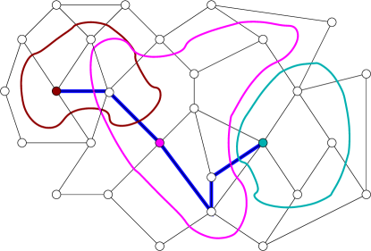
$\omega$ $x_{0}$ $S_{\omega,x_{0}}$ $x_{1}^{\prime}$ $x_{1}$ $S_{\omega,x_{1}}$ $x_{2}^{\prime}$ $x_{2}$ $S_{\omega,x_{2}}$

Figure 2.1: A “good path” that gives the vertex $(x_{0},x_{1},x_{2})$ of $T^{\omega}$.

Let $T^{\omega}(p)$ be the random subtree of $T^{\omega}$ defined in a similar way but allowing only good paths that are open in Bernoulli($p$) percolation on ${\omega}$. It is easy to check that in fact $T^{\omega}(p)\subseteq T^{\omega}$. Denote by $L_{n}(p)$ the set of vertices of $T^{\omega}(p)$ in the $n$th level. A self-avoiding infinite ray inside the $p$-percolation configuration gives rise to a growing sequence of good paths in the percolated ${\omega}$, therefore if the cluster of the origin in the $p$-percolation on ${\omega}$ is infinite, then there is an infinite path in $T^{\omega}(p)$. Conversely, an infinite path in $T^{\omega}(p)$ corresponds to an infinite growing sequence of open good paths in the $p$-percolated ${\omega}$, which are necessarily parts of an infinite component containing the origin.

We claim that for almost every ${\omega}$ the expected number of vertices in $L_{n}(p)$ converges to 0 as $n\to\infty$. More precisely, the expectation of the number of vertices in $L_{n}(p)$ decreases exponentially in $n$. In the first two inequalities we use the notation $\square$ for the occurence of events on disjoint edge sets and we apply the BK inequality ([16], Theorem 2.12). We denote the event $\Big{\{}x_{0}\xleftrightarrow[B]{{\omega},p}x_{k}\textrm{ by a good path through }x_{0},x_{1},\dots,x_{k}\Big{\}}$ by $\Big{\{}x_{0}\xleftrightarrow[B,(x_{0},x_{1},\dots,x_{k})]{{\omega},p}x_{k}\Big{\}}$.

$$\mathrm{\mathbb{E}}^{\omega}\big{(}|L_{n}(p)|\big{)} =\sum_{(x_{0},\dots,x_{n})\in L_{n}}\mathrm{\mathbb{P}}^{\omega}\left(x_{0}\xleftrightarrow[S,(x_{0},\dots,x_{n})]{{\omega},p}x_{n}\right)$$

$$\leq\sum_{\begin{subarray}{c}(x_{0},\dots,x_{n-1})\in L_{n-1}\\ e\in\partial_{E}S_{{\omega},x_{n-1}}\end{subarray}}\mathrm{\mathbb{P}}^{\omega}\left(\Big{\{}x_{0}\xleftrightarrow[S,(x_{0},\dots,x_{n-1})]{{\omega},p}x_{n-1}\Big{\}}\square\big{\{}e\textrm{ is open}\big{\}}\square\Big{\{}x_{n-1}\xleftrightarrow[S_{{\omega},x_{n-1}}]{{\omega},p}e^{-}\Big{\}}\right)$$

$$\leq\sum_{\begin{subarray}{c}(x_{0},\dots,x_{n-1})\in L_{n-1}\\ e\in\partial_{E}S_{{\omega},x_{n-1}}\end{subarray}}\mathrm{\mathbb{P}}^{\omega}\left(x_{0}\xleftrightarrow[S,(x_{0},\dots,x_{n-1})]{{\omega},p}x_{n-1}\right)p\,\mathrm{\mathbb{P}}^{\omega}\bigg{(}x_{n-1}\xleftrightarrow[S_{{\omega},x_{n-1}}]{{\omega},p}e^{-}\bigg{)}$$

$$=\sum_{(x_{0},\dots,x_{n-1})\in L_{n-1}}\mathrm{\mathbb{P}}^{\omega}\left(x_{0}\xleftrightarrow[S,(x_{0},\dots,x_{n-1})]{{\omega},p}x_{n-1}\right)\phi_{p}^{{\omega},x_{n-1}}(S_{{\omega},x_{n-1}})\leq\mathrm{\mathbb{E}}^{\omega}\left(|L_{n-1}(p)|\right)c\,.$$

It follows by induction that $\mathrm{\mathbb{E}}^{\omega}\big{(}|L_{n}(p)|\big{)}\leq c^{n}$. Therefore,

$$\mathrm{\mathbb{P}}^{\omega}(|\mathcal{C}_{o}|=\infty)=\mathrm{\mathbb{P}}^{\omega}(T^{\omega}(p)\textrm{ survives})=\lim_{n\to\infty}\mathrm{\mathbb{P}}^{\omega}(|L_{n}(p)|\geq 1)\leq\lim_{n\to\infty}\mathrm{\mathbb{E}}^{\omega}|L_{n}(p)|=0\,,$$

hence $p\leq{p_{c}}$.

Next we prove that ${\tilde{p}_{c}}\geq{p_{c}}$. Let

$$q(p):=\mu(\big{\{}{\omega}:\phi^{\omega}_{p}(S)\geq 1\textrm{ for all }S\in\mathcal{S}({\omega})\}\big{)},$$

Note that $q(p)$ is non-decreasing in $p$, and $q(p)>0$ for every $p>{\tilde{p}_{c}}$ by the definition of ${\tilde{p}_{c}}$.

Fix ${\omega}$ and let $H\in\mathcal{S}({\omega})$ be fixed. We will use Lemma 1.4. of [11]:

$$\frac{d}{dp}\mathrm{\mathbb{P}}_{p}^{\omega}\left(o\xleftrightarrow{{\omega},p}H^{c}\right)\geq\left(1-\mathrm{\mathbb{P}}_{p}^{\omega}\left(o\xleftrightarrow{H,p}H^{c}\right)\right)\inf_{S:o\in S\subseteq H}\phi_{p}^{H}(S)\geq C(p)\inf_{S:o\in S\subseteq H}\phi_{p}^{H}(S)\,,$$

where $C(p)=(1-p)^{D}\leq 1-\mathrm{\mathbb{P}}^{\omega}\left(o\xleftrightarrow{{\omega},p}H^{c}\right)$ for every ${\omega}$ and $H$, with $D$ being the almost sure bound on the degree of the graph $G$. The probabilities above depend only on the structure of ${\omega}$ in $K=H\cup\partial_{V}^{\mathrm{out}}H$, hence we can use the above inequality to estimate the derivative of the probability $\mu\left(o\xleftrightarrow{{\omega},p}B^{\omega}(o,r)^{c}\right)$, as follows. Consider the following sets of finite rooted graphs: let $\mathcal{H}_{r}$ be the set of possible $(r+1)$-neighbourhoods of the graphs with degree at most $D$, i.e.

$$\mathcal{H}_{r}:= \left\{(K,o):\mathrm{dist}_{K}(o,x)\leq r+1\textrm{ and }\mathrm{deg}_{K}(x)\leq D\,,\textrm{ for all }x\in V(K)\right\},$$

and let

$$\mathcal{H}_{r}(p):= \left\{(K,o)\in\mathcal{H}_{r}:\phi_{p}^{K}(S)\geq 1\,,\textrm{ for all }S\in\mathcal{S}(B_{K}(o,r))\right\}.$$

Note that

$$\sum_{K\in\mathcal{H}_{r}(p)}\mu\left(\left\{{\omega}:B_{\omega}(o,r+1)=K\right\}\right) =$$

$$\mu(\big{\{}{\omega}:\phi^{\omega}_{p}(S)\geq 1\textrm{ for all }S\in\mathcal{S}(B_{{\omega}}(o,r))\}\big{)} \geq q(p),$$

hence we have

$$\frac{d}{dp}\mu\left(o\xleftrightarrow{{\omega},p}B(o,r)^{c}\right) =\sum_{(K,o)\in\mathcal{H}_{r}}\mu\big{(}B_{\omega}(o,r+1)=K\big{)}\frac{d}{dp}\mathrm{\mathbb{P}}_{p}\left(o\xleftrightarrow{K,p}B_{K}(o,r)^{c}\right)$$

$$\geq\sum_{(K,o)\in\mathcal{H}_{r}(p)}\mu\big{(}B_{\omega}(o,r+1)=K\big{)}C(p)\inf_{S:o\in S\subseteq B_{K}(o,r)}\phi_{p}^{K}(S)$$

$$\geq q(p)\,C(p).$$

Integrate the above inequality on the interval $\left[\frac{p+{\tilde{p}_{c}}}{2},p\right]$. Using the monotonicity of $q(p)$ and $C(p)$, we get

$$\mu\left(o\xleftrightarrow{{\omega},p}B(o,r)^{c}\right)\geq\frac{p-{\tilde{p}_{c}}}{2}\,q\left(\frac{p+{\tilde{p}_{c}}}{2}\right)C(p).$$

This gives a positive lower bound that is uniform in $r$. Thus $\mu\left(o\xleftrightarrow{{\omega},p}\infty\right)>0$, and $p\geq{p_{c}}$. $\blacksquare$

One advantage of the definition of ${\tilde{p}_{c}}$ for transitive graphs is that it enables one to check whether a certain $p$ is under ${\tilde{p}_{c}}$ using a finite witness. This characteristic makes the next definition natural.

Definition 2.1.

We say that a bounded degree unimodular random graph $G$ is uniformly good if for any $p<{p_{c}}$ there exists a positive integer $r(p)$ such that $\mu_{G}(\{{\omega}:\exists S_{\omega}\subseteq B_{\omega}(o,r(p)),o\in S_{\omega}\textrm{ s.t. }\phi_{p}^{\omega}(S_{\omega})<1\})=1$ .

This class of graphs includes unimodular quasi-transitive graphs (obvious) and unimodular random trees of uniform sub-exponential growth (see Definition 2.4 and the proof of Proposition 1.4 in Subsection 3.2). Furthermore, uniformly good unimodular graphs satisfy the following exponential decay of $\phi_{p}(B_{\omega}(o,r))$ in $r$.

Lemma 2.2.

Let $G$ be a bounded degree unimodular random graph. $G$ is uniformly good if and only if for all $p<{p_{c}}$ there are constants $c=c(p)<1$ and $R(p)$ such that if $r\geq R(p)$, then $\phi_{p}^{\omega}(B)\leq c^{r}$ for almost every ${\omega}$ and every finite $B\supseteq B_{\omega}(o,r)$.

For the proof of Lemma 2.2 we use the same tree $T^{\omega}$ as in the proof of Theorem 1.1. The uniformly good property implies a uniform linear lower bound in $r$ on the distance of the root from any vertex of $T^{\omega}$ that corresponds to a boundary point of $B$ (namely the points of the set $\pi$ defined in the proof). This property and the boundedness of the size of the sets $S_{{\omega},x}$ allows us to prove the estimate of the lemma.

Proof. If the constants $c(p)$ and $R(p)$ exist, then the sets $S_{\omega}:=B_{\omega}(o,R(p))$ indicate that $G$ is uniformly good.

To prove the other direction, assume that $G$ is uniformly good, and fix $p<{p_{c}}$. We can show as in the proof of Theorem 1.1 that there exists a constant $c_{0}<1$ and a positive integer $r_{0}$ such that for almost every ${\omega}$ and every $x\in{\omega}$ there exists a finite connected set $S_{{\omega},x}\subseteq B_{\omega}(x,r_{0})$ containing $x$ that satisfies $\phi_{p}^{{\omega},x}(S_{{\omega},x})\leq c_{0}$. Fix an ${\omega}$ and the sets $S_{{\omega},x}$ as above, a positive integer $r$ and a finite set $B\supseteq B_{\omega}(o,r)$. We define the trees $T^{\omega}$ and $T^{\omega}(p)$ as in the proof of Theorem 1.1. On every directed path in $T^{\omega}$ from $o$ to infinity there is a first vertex $(x_{0},\dots,x_{k})$ such that $x_{k}\notin B$. Let $\pi$ be the set of these vertices, i.e.

$$\pi:=\{(x_{0},\dots,x_{k})\in T^{\omega}:x_{0},\dots,x_{k-1}\in B,x_{k}\notin B\}.$$

Note that $\pi$ is a minimal set in $T^{\omega}$ that separates $o$ from infinity, hence every non-backtracking infinite path from $o$ has exactly one vertex in $\pi$. An argument as in the first part of the proof of Theorem 1.1 shows that

$$\mathrm{\mathbb{E}}^{\omega}\left(|\pi\cap T^{\omega}(p)|\right) =\sum_{(x_{0},\dots,x_{k})\in\pi}\mathrm{\mathbb{P}}^{\omega}\Big{(}x_{0}\xleftrightarrow[B,(x_{0},\dots,x_{k})]{{\omega},p}x_{k}\Big{)}$$

$$\leq\sum_{(x_{0},\dots,x_{k})\in\pi}\sum_{(x^{\prime}_{1},\dots,x^{\prime}_{k})}\prod_{j=1}^{k}\mathrm{\mathbb{P}}^{\omega}\Big{(}x_{j-1}\xleftrightarrow[S_{{\omega},x_{j-1}}]{{\omega},p}x_{j}^{\prime}\Big{)}p=:F(\pi,p),$$

where $(x^{\prime}_{1},\dots,x^{\prime}_{k})$ denotes a sequence of vertices in ${\omega}$ such that $x_{j}^{\prime}\in S_{{\omega},x_{j-1}}$ and $x_{j}^{\prime}\sim x_{j}$ for any $j=1,\dots,k$. First we bound $\phi_{p}^{\omega}(B)$ in terms of $F(\pi,p)$ using the uniform bound on the size of the sets $S_{{\omega},x}$, then we prove a geometric bound on $F(\pi,p)$ using a linear bound in $r$ on the distance of $o$ and $\pi$ in $T^{\omega}$. These two estimates will imply the statement of the lemma.

Denote by $\bar{\pi}$ the set of the parents of the vertices in $\pi$, i.e.

$$\bar{\pi}:=\{(x_{0},\dots,x_{k})\in T^{\omega}:x_{0},\dots,x_{k}\in B,\exists x_{k+1}\notin B,(x_{0},\dots,x_{k+1})\in T^{\omega}\}.$$

If for some $e\in\partial_{E}B$ the event $\big{\{}o\xleftrightarrow[B]{{\omega},p}e^{-}\big{\}}$ occurs, then there is some $(x_{0},\dots,x_{k})\in\bar{\pi}$ such that there is a good path through $x_{0},\dots,x_{k}$ in the percolation and a disjoint path from $x_{k}$ to $e^{-}$ in $S_{{\omega},x_{k}}$. For any fixed $(x_{0},\dots,x_{k})$ the number of edges in $\partial_{E}B\cap\left(E(S_{{\omega},x_{k}})\cup\partial_{E}S_{{\omega},x_{k}}\right)$ is bounded above by $|E(S_{{\omega},x_{k}})\cup\partial_{E}S_{{\omega},x_{k}}|\leq D^{r_{0}+1}$ where $D$ is the almost sure bound on the degree of the graph $G$. We have

$$\phi_{p}^{\omega}(B) =p\sum_{e\in\partial_{E}B}\mathrm{\mathbb{P}}^{\omega}\Big{(}o\xleftrightarrow[B]{{\omega},p}e^{-}\Big{)}$$

$$\leq\sum_{e\in\partial_{E}B}\sum_{\begin{subarray}{c}(x_{0},\dots,x_{k})\in\bar{\pi}\\ (x^{\prime}_{0},\dots,x^{\prime}_{k})\end{subarray}}\mathrm{\mathbb{P}}_{p}^{\omega}\left(\Big{\{}x_{0}\xleftrightarrow[B,(x_{0},\dots,x_{k})]{{\omega},p}x_{k}\Big{\}}\square\Big{\{}x_{k}\xleftrightarrow[S_{{\omega},x_{k}}]{{\omega},p}e^{-}\Big{\}}\right)$$

$$\leq\sum_{\begin{subarray}{c}(x_{0},\dots,x_{k})\in\bar{\pi}\\ (x^{\prime}_{0},\dots,x^{\prime}_{k})\end{subarray}}\bigg{(}\prod_{j=1}^{k}\mathrm{\mathbb{P}}^{\omega}\Big{(}x_{j-1}\xleftrightarrow[S_{{\omega},x_{j-1}}]{{\omega},p}x_{j}^{\prime}\Big{)}p\bigg{)}\sum_{e\in\partial_{E}B\cap\left(E(S_{{\omega},x_{k}})\cup\partial_{E}S_{{\omega},x_{k}}\right)}\mathrm{\mathbb{P}}_{p}^{\omega}\Big{(}x_{k}\xleftrightarrow[S_{{\omega},x_{k}}]{{\omega},p}e^{-}\Big{)}$$

$$\leq\sum_{\begin{subarray}{c}(x_{0},\dots,x_{k})\in\bar{\pi}\\ (x^{\prime}_{0},\dots,x^{\prime}_{k})\end{subarray}}\bigg{(}\prod_{j=1}^{k}\mathrm{\mathbb{P}}^{\omega}\Big{(}x_{j-1}\xleftrightarrow[S_{{\omega},x_{j-1}}]{{\omega},p}x_{j}^{\prime}\Big{)}p\bigg{)}D^{r_{0}+1}=F(\bar{\pi},p)D^{r_{0}+1}.$$ (2.2)

To estimate (2.2), note that

$$F(\pi,p) =\sum_{\begin{subarray}{c}(x_{0},\dots,x_{k})\in\bar{\pi}\\ (x^{\prime}_{0},\dots,x^{\prime}_{k})\end{subarray}}\bigg{(}\prod_{j=1}^{k}\mathrm{\mathbb{P}}^{\omega}\Big{(}x_{j-1}\xleftrightarrow[S_{{\omega},x_{j-1}}]{{\omega},p}x_{j}^{\prime}\Big{)}p\bigg{)}\sum_{\begin{subarray}{c}x_{k+1}:(x_{0},\dots,x_{k+1})\in\pi\\ x^{\prime}_{k+1}\in S_{{\omega},x_{k}},x^{\prime}_{k+1}\sim x_{k+1}\end{subarray}}\mathrm{\mathbb{P}}^{\omega}\Big{(}x_{k}\xleftrightarrow[S_{{\omega},x_{k}}]{{\omega},p}x_{k+1}^{\prime}\Big{)}p$$

$$\geq\sum_{\begin{subarray}{c}(x_{0},\dots,x_{k})\in\bar{\pi}\\ (x^{\prime}_{0},\dots,x^{\prime}_{k})\end{subarray}}\bigg{(}\prod_{j=1}^{k}\mathrm{\mathbb{P}}^{\omega}\Big{(}x_{j-1}\xleftrightarrow[S_{{\omega},x_{j-1}}]{{\omega},p}x_{j}^{\prime}\Big{)}p\bigg{)}p^{r_{0}+1}=F(\bar{\pi},p)p^{r_{0}+1}$$

by the assumption that the graph is uniformly good. Combined this with (2.2) gives

$$\phi_{p}^{\omega}(B) \leq\frac{D^{r_{0}+1}}{p^{r_{0}+1}}F(\pi,p).$$ (2.3)

Now we show that $F(\pi,p)\leq c_{0}^{\frac{r}{r_{0}}}$, which combined with (2.3) proves the lemma. Let $\pi_{n}:=\bigcup_{m\leq n}\left(\pi\cap L_{m}\right)\cup\left\{v\in L_{n}:v\textrm{ has a descendant in }\pi\right\}$, which is a minimal vertex set that separates the root from infinity. Let $R:=\max\{n:L_{n}\cap\pi\neq\emptyset\}<\infty$, thus $\pi=\pi_{R}$. Note that each $\pi_{n}$ is the disjoint union of $\pi_{n+1}\setminus L_{n+1}\subseteq\pi$ and $\pi_{n}\setminus\pi_{n+1}\subseteq L_{n}$. We estimate $F(\pi,p)$ by summing over a larger set: the union of $\pi_{R}\setminus L_{R}$ and $\{(x_{0},\dots,x_{R}):(x_{0},\dots,x_{R-1})\in\pi_{R-1}\setminus\pi_{R},x_{R}\in\partial_{V}^{\mathrm{out}}S_{{\omega},x_{R-1}}\}\supseteq\pi_{R}\cap L_{R}$. That is, using the bound

$$\sum_{e\in\partial_{E}S_{{\omega},x_{R-1}}}\mathrm{\mathbb{P}}^{\omega}\Big{(}x_{R-1}\xleftrightarrow[S_{{\omega},x_{R-1}}]{{\omega},p}e^{-}\Big{)}p=\phi_{p}^{{\omega},x_{R-1}}(S_{{\omega},x_{R-1}})\leq 1$$

for the second term in the following estimation, we have

$$F(\pi,p) \leq\sum_{(x_{0},\dots,x_{k})\in\pi_{R}\setminus L_{R}}\sum_{(x^{\prime}_{1},\dots,x^{\prime}_{k})}\prod_{j=1}^{k}\mathrm{\mathbb{P}}^{\omega}\Big{(}x_{j-1}\xleftrightarrow[S_{{\omega},x_{j-1}}]{{\omega},p}x_{j}^{\prime}\Big{)}p$$

$$+\sum_{\begin{subarray}{c}(x_{0},\dots,x_{R-1})\in\pi_{R-1}\setminus\pi_{R}\\ (x^{\prime}_{1},\dots,x^{\prime}_{R-1})\end{subarray}}\bigg{(}\prod_{j=1}^{R-1}\mathrm{\mathbb{P}}^{\omega}\Big{(}x_{j-1}\xleftrightarrow[S_{{\omega},x_{j-1}}]{{\omega},p}x_{j}^{\prime}\Big{)}p\bigg{)}\sum_{e\in\partial_{E}S_{{\omega},x_{R-1}}}\mathrm{\mathbb{P}}^{\omega}\Big{(}x_{R-1}\xleftrightarrow[S_{{\omega},x_{R-1}}]{{\omega},p}e^{-}\Big{)}p$$

$$\leq\sum_{(x_{0},\dots,x_{k})\in\pi_{R-1}}\sum_{(x^{\prime}_{1},\dots,x^{\prime}_{k})}\prod_{j=1}^{k}\mathrm{\mathbb{P}}^{\omega}\Big{(}x_{j-1}\xleftrightarrow[S_{{\omega},x_{j-1}}]{{\omega},p}x_{j}^{\prime}\Big{)}p=F(\pi_{R-1},p).$$

A similar argument shows that $F(\pi,p)\leq F(\pi_{n},p)$ for any $n\leq R$. If $(x_{0},\dots,x_{k})\in\pi$, then ${\mathop{\textrm{dist}}}_{\omega}(o,x_{k})\geq r$, hence the distance between $o$ and $\pi$ in $T^{\omega}$ is at least $\frac{r}{r_{0}}$, thus $\pi_{n}=L_{n}$ for any $n\leq\frac{r}{r_{0}}$. If we apply the above argument for $F(\pi_{n},p)$ whith $n\leq\frac{r}{r_{0}}$, then the first term disappear, and the inequality $\phi_{p}^{{\omega},x_{n-1}}(S_{{\omega},x_{n-1}})\leq c_{0}$ gives

$$F(\pi,p)\leq F(\pi_{\frac{r}{r_{0}}},p)\leq F(\pi_{\frac{r}{r_{0}}-1},p)c_{0}\leq\dots\leq c_{0}^{\frac{r}{r_{0}}}\,.$$

This combined with (2.3) proves the lemma. $\blacksquare$

Corollary 2.3.

If $G$ is a uniformly good unimodular graph, then ${p_{c}}\leq\tilde{p}_{c}^{\mathsf{a}}$.

Proof. Let $p<{p_{c}}$, and let $c$ and $R(p)$ be as in Lemma 2.2. We have $\mathrm{\overline{\mathbb{E}}}\left(\phi_{p}^{\omega}\left(B_{\omega}(o,R(p))\right)\right)\leq c^{R}<1$, thus $p\leq\tilde{p}_{c}^{\mathsf{a}}$. $\blacksquare$

We will see in Remark 2.9 that, without the assumption of uniform goodness, the inequality ${p_{c}}\leq\tilde{p}_{c}^{\mathsf{a}}$ does not necessarily hold. Also, we will show in Example 2.11 that there are uniformly good graphs with ${p_{c}}<\tilde{p}_{c}^{\mathsf{a}}$.

Definition 2.4.

A random rooted graph $(G,o)$ has uniform sub-exponential volume growth if for any $c<1$ and $\varepsilon>0$ there is an $R$ such that $\mu\left({\omega}:|B_{\omega}(o,r)|c^{r}<\varepsilon\right)=1$ for any $r>R$.

Corollary 2.5.

If $G$ is a uniformly good unimodular graph with uniform sub-exponential volume growth, then ${p_{c}}={p_{T}}={p_{T}^{\mathsf{a}}}$.

Proof. Let $p<{p_{c}}={\tilde{p}_{c}}$ and let $c$ and $R(p)$ be as in Lemma 2.2. Denote by $D$ the maximum degree of $G$. Let $R>R(p)$ such that $\mu\left(\{{\omega}:|B_{\omega}(o,r)|c^{r/2}<1\}\right)=1$ for any $r>R$ and let ${\omega}$ satisfy this event for all $r>R$ simultaneously. Then we have

$$\mathrm{\mathbb{E}}_{p}^{\omega}\left(|\mathcal{C}_{o}|\right) =\sum_{n=1}^{\infty}\mathrm{\mathbb{P}}^{\omega}_{p}\left(|\mathcal{C}_{o}|\geq n\right)=\sum_{r=1}^{\infty}\sum_{n=|B_{\omega}(o,r)|+1}^{|B_{\omega}(o,r+1)|}\mathrm{\mathbb{P}}^{\omega}_{p}\left(|\mathcal{C}_{o}|\geq n\right)$$

$$\leq\sum_{r=1}^{\infty}\sum_{n=|B_{\omega}(o,r)|+1}^{|B_{\omega}(o,r+1)|}\mathrm{\mathbb{P}}^{\omega}_{p}\left(o\xleftrightarrow{p,{\omega}}B_{\omega}(o,r)^{c}\right)$$

$$\leq\sum_{r=1}^{\infty}|B_{\omega}(o,r+1)|\min\{\phi^{\omega}_{p}\left(B_{\omega}(o,r)\right),1\}$$

$$\leq\sum_{r=2}^{R+1}|B_{\omega}(o,r)|+\sum_{r=R+1}^{\infty}|B_{\omega}(o,r+1)|c^{r}$$

$$\leq\sum_{r=2}^{R+1}D^{r}+\sum_{r=R+1}^{\infty}c^{r/2}<\infty$$

This gives a uniform upper bound on $\mathrm{\mathbb{E}}_{p}^{\omega}\left(|\mathcal{C}_{o}|\right)$ thus $\mathrm{\overline{\mathbb{E}}}_{p}\left(|\mathcal{C}_{o}|\right)<\infty$. It follows that $p\leq{p_{T}^{\mathsf{a}}}$, hence ${p_{T}^{\mathsf{a}}}\geq{p_{c}}$. The other direction follows from the definition of ${p_{T}^{\mathsf{a}}}$. $\blacksquare$

Subexponential volume growth also appears in Theorem 1.4, Example 3.6 and Corollary 4.1.

2.2 Counterexamples

We show in Examples 2.8 and 2.10 that there are unimodular random graphs of uniform subexponential (in fact, quadratic) volume growth, but ${p_{T}}<{p_{c}}$ and ${p_{T}^{\mathsf{a}}}<{p_{T}}$. Both constructions will use Bernoulli percolation on $\mathbb{Z}^{2}$ as an ingredient; moreover, although we define the graph in the second example as a vertex replacement of $\mathbb{Z}^{2}$, it could be defined even as an invariant random subgraph of $\mathbb{Z}^{2}$. We further give examples of graphs with $\tilde{p}_{c}^{\mathsf{a}}<{p_{c}}$ and $\tilde{p}_{c}^{\mathsf{a}}>{p_{c}}$; see Examples 2.9 and 2.11, respectively. First we need a lemma that will be useful in our examples.

Lemma 2.6.

For any $\varepsilon>0$ there is a probability $p_{1}<1$ such that for $n$ large enough, the vertices $(0,-n)$, $(0,n)$, $(-n,0)$, $(n,0)$ are in the same cluster in Bernoulli($p_{1}$) percolation on $Q_{n}$ with probability at least $1-\varepsilon$.

Proof. The occurrence of the events in the following two claims implies the occurrence of the event in the statement of the lemma, hence we will be done by a union bound.

Claim 1: For any $p>{1}/{2}$ and $n>n_{0}(p,\varepsilon)$ large enough, in Bernoulli($p$) percolation on $Q_{n}$, with probability at least $1-\varepsilon/2$, there is a giant cluster with the following properties: it joins all the sides of $Q_{n}$, while every other cluster in $Q_{n}$ has diameter at most ${n}/{5}$. This was proved in [3, Proposition 2.1].

Claim 2: There exists $p_{1}<1$ such that for all $n$ and all $p>p_{1}$,

$$\mathrm{\mathbb{P}}_{p}\left(\mathrm{diam}(\mathcal{C}_{(0,n)})\geq n\right)\geq 1-\varepsilon/8\,.$$

Similarly for $(0,-n)$, $(-n,0)$, and $(n,0)$, instead of $(0,n)$. The proof follows from a standard Peierls contour argument, thus we leave it to the reader. $\blacksquare$

We will use the following unimodular random graph, the canopy tree, in several of our examples. It is the local weak limit of large balls in the 3-regular tree:

Definition 2.7 (Busemann functions and canopy tree).

Let $\mathbb{T}$ be the 3-regular infinite tree with a root $o$, a distinguished end $\xi$, and a Busemann function (see [32]) $\mathfrak{h}:\mathbb{T}\to\mathbb{Z}$ that gives the levels w.r.t. to $\xi$. More precisely, to define $\mathfrak{h}$, for any vertex $x$, let $(\xi,x)$ be the unique infinite simple path from $x$ which is in the equivalence class $\xi$. Denote by $x\wedge o$ the unique vertex in $\mathbb{T}$ such that $(\xi,x\wedge o)=(\xi,x)\cap(\xi,o)$, i.e., the first vertex where $(\xi,x)$ and $(\xi,o)$ coalesce. Finally, let $\mathfrak{h}(x):={\mathop{\textrm{dist}}}(o,x\wedge o)-{\mathop{\textrm{dist}}}(x,x\wedge o)$.

Let $\Lambda\subset\mathbb{T}$ be the subgraph spanned by the vertices $x$ with $\mathfrak{h}(x)\geq 0$. This tree $\Lambda$ is called the canopy tree. Denote by $L(n):=\{x\in V(\mathbb{T}):\mathfrak{h}(x)=n\}$ the $n^{\textrm{th}}$ vertex level and by $L_{E}(n):=\{e\in E(\mathbb{T}):e^{-}\in L(n),e^{+}\in L(n+1)\}$ the $n^{\textrm{th}}$ edge level of $\mathbb{T}$, or, for $n\geq 0$, of $\Lambda$. If we choose the root $o$ of $\Lambda$ such that $\mathrm{\mathbb{P}}(o\in L(n))=2^{-n-1}$, we get a unimodular random graph.

Example 2.8.

There is a unimodular graph with uniform polynomial volume growth and ${p_{T}}<{p_{c}}$. In particular, the exponential decay of two-point connection probabilities fails for $p\in({p_{T}},{p_{c}})$ on this graph.

Proof. We define the graph $G$ as an edge replacement (see [2], Example 9.8) of the canopy tree: each $e\in L_{E}(n)$ is replaced by $(Q_{2^{n}}(e),(0,-{2^{n}}),(0,{2^{n}}))$, where $Q_{2^{n}}(e)$ is isomorphic to $Q_{2^{n}}$. It is easy to see that the volume of $B_{G}(o,r)$, for any root $o$ and radius $r$, is at most $Cr^{2}$, for some absolute constant $C<\infty$. Indeed, if the root is in $Q_{2^{n}}(e)$, then $B_{G}(o,r)$ intersects the cubes $Q_{2^{l}}(e^{\prime})$ with $e^{\prime}\in(\xi,e)$ only if $l\leq\log_{2}r$ or $l=n$. Furthermore, each such $Q_{2^{l}}(e^{\prime})$ has more vertices than the sum of the number of vertices of $Q_{2^{k}}(e^{\prime\prime})$ with $e^{\prime}\in(\xi,e^{\prime\prime})$, which are the further cubes that may intersect $B_{G}(o,r)$. It follows that $|B_{G}(o,r)|\leq\min\left\{r^{2},\sum_{l=n}^{\log_{2}r}2^{2l+3}\right\}\leq Cr^{2}$.

We will now show that ${p_{T}}(G)<{p_{c}}(G)=1$. Consider Bernoulli($p$) percolation $\omega$ on $G$ and, as a deterministic function of it, define the following percolation $\lambda$ on $\Lambda$: an edge $e\in L_{E}(n)$ is open in $\lambda$ if and only if the vertices $(0,-n)$ and $(0,n)\in Q_{n}(e)$ are connected by an open path in $\omega$. Clearly, there exists an infinite cluster in $\omega$ if and only if there is an infinite cluster in $\lambda$. The law of $\lambda$ is stochastically dominated by a Bernoulli($1-(1-p)^{3}$) percolation on $\Lambda$, because if $e\in L_{E}(n)$ is open, then at least one of the edges in $Q_{n}(e)$ adjacent to $(0,n)$ is open. The tree $\Lambda$ has one end, hence, for any $p<1$,

$$\mathrm{\mathbb{P}}_{p}^{G}(\exists\text{ an infinite cluster})\leq\mathrm{\mathbb{P}}_{1-(1-p)^{3}}^{\Lambda}(\exists\text{ an infinite cluster})=0\,.$$

That is, ${p_{c}}(G)=1$.

An easy first moment computation (that we omit) shows that ${p_{T}}(\Lambda)={1}/{\sqrt{2}}$. Now let $0<\varepsilon<1-{1}/{\sqrt{2}}$. It follows from Lemma 2.6 that there exists $p_{1}<1$ and some large $N$ such that $\mathrm{\mathbb{P}}_{p_{1}}(e\in\lambda)\geq 1-\varepsilon$ for all $e\in L_{E}(n)$ with $n\geq N$. Thus, for $o\in L(N)$, the cluster $\mathcal{C}_{o}$ in $\lambda$, restricted to the levels $n\geq N$, stochastically dominates Bernoulli($1-\varepsilon$) percolation on $\Lambda$. The latter has infinite expected size, hence the expected size of the cluster in $\omega$ of $(0,-N)\in Q_{N}(e)$ for $e\in L_{E}(N)$ is also infinite. That is, ${p_{T}}(G)\leq p_{1}<1$. $\blacksquare$

Example 2.9.

The canopy tree $\Lambda$ (see Definition 2.7) satisfies $\tilde{p}_{c}^{\mathsf{a}}=\frac{1}{\sqrt{2}}$, thus this is an example of a not uniformly good unimodular graph with ${p_{c}}>\tilde{p}_{c}^{\mathsf{a}}$.

Proof. It is easy to check that $\mathrm{\overline{\mathbb{E}}}(\phi_{p}(B(o,r)))$ equals $2p(\sqrt{2}p)^{r}$ if $r$ is even, and equals $3(\sqrt{2}p)^{r+1}/2$ if $r$ is odd. This sequence converges to 0 for $p<1/\sqrt{2}$, while remains above 1 for $p>1/\sqrt{2}$, which implies the claim. $\blacksquare$

Example 2.10.

There is a unimodular graph with polynomial volume growth and ${p_{T}^{\mathsf{a}}}<{p_{T}}$.

Proof. Let $X$ be a positive integer valued random variable such that $\mathrm{\mathbb{P}}(X=k)=ck^{-5/2}$ for all $k\geq 1$. Then $\mathrm{\mathbb{E}}X<\infty$ and $\mathrm{\mathbb{E}}(X^{2})=\infty$. We define the graph $G$ as a vertex replacement (see Subsection 1.4) of $\mathbb{Z}^{2}$ with respect to the following labels as follow. Let $\{X_{n},X^{\prime}_{n}:n\in\mathbb{Z}\}$ be iid copies of $X$, and for each vertex $(m,n)\in\mathbb{Z}^{2}$, let $G_{(m,n)}$ be isomorphic to the subgraph of $\mathbb{Z}^{2}$ spanned by the vertices in $[0,2X_{m}]\times[0,2X^{\prime}_{n}]$, and for the edges going from $(m,n)$ to North, East, South, and West, let the image of $\varphi_{(m,n)}$ be the corresponding midpoint of the box $G_{(m,n)}$. We can also think of the resulting graph as an invariant random subgraph of $\mathbb{Z}^{2}$.

Denote by $Y$ and $Y^{\prime}$ half the length of the sides of the box of $o$ in $G$, i.e., the law of $X_{0}$ and $X^{\prime}_{0}$ biased by $X_{0}X^{\prime}_{0}$. Then

$$\mathrm{\mathbb{P}}(Y=k,Y^{\prime}=l)=\frac{kl}{(\mathrm{\mathbb{E}}X)^{2}}\mathrm{\mathbb{P}}(X=k,X^{\prime}=l),$$

hence $Y$ and $Y^{\prime}$ are independent with distribution $\mathrm{\mathbb{P}}(Y=k)=\frac{ck^{-3/2}}{\mathrm{\mathbb{E}}X}$.

First we show that ${p_{T}^{\mathsf{a}}}=\frac{1}{2}$. $G$ is a subgraph of $\mathbb{Z}^{2}$, hence ${p_{T}^{\mathsf{a}}}(G)\geq\frac{1}{2}$. Fix $p>\frac{1}{2}$ and let $\varepsilon>0$. Denote by $M(Q_{n})$ the largest cluster in percolation with parameter $p$ in the box $Q_{n}$, and let

$$\mathcal{A}(Q_{n}):=\big{\{}|M(Q_{n})|\geq(1-\varepsilon)\theta(p)|Q_{n}|,\quad\mathrm{diam}(C)<\nu\log n\ \forall\textrm{ open cluster }C\neq M(Q_{n})\big{\}},$$

where $\theta(p)=\mathrm{\mathbb{P}}_{p}(|\mathcal{C}_{o}(\mathbb{Z}^{2})|=\infty)$, and $\nu$ is chosen as follows: by [16, Theorem 7.61], there is an $N=N(p)$ and $\nu=\nu(p)$ such that, for any $n\geq N$,

$$\mathrm{\mathbb{P}}_{p}(\mathcal{A}(Q_{n}))>1-\varepsilon\,.$$

Let $Z:=\min\{Y,Y^{\prime}\}$, and consider the event $\mathcal{D}(G_{0,0}):=\left\{{\mathop{\textrm{dist}}}(o,\partial_{V}^{\mathrm{in}}G_{0,0})\geq\nu\log Z\right\}$. If $Z$ is large enough, then $\mathrm{\mathbb{P}}\big{(}\mathcal{D}(G_{0,0})\,\big{|}\,Z\big{)}\geq 1-\varepsilon$, since $o$ is uniform in $G_{0,0}$. Assuming that $\mathcal{D}(G_{0,0})$ occurs, choose a box $Q_{Z}\subseteq G_{0,0}$ that contains $o$ such that ${\mathop{\textrm{dist}}}(o,\partial_{V}^{\mathrm{in}}Q_{Z})\geq\nu\log Z$. Consider percolation on $\mathbb{Z}^{2}\supset Q_{Z}$. If $o$ is in the unique infinite cluster of this percolation on $\mathbb{Z}^{2}$, then the diameter of $\mathcal{C}_{o}(Q_{Z})$ is at least $\nu\log Z$, hence

$$\mathrm{\mathbb{P}}_{p}\Big{(}o\in M(Q_{Z}),\mathcal{A}(Q_{Z})\,\Big{|}\,Z=n,\mathcal{D}(G_{0,0})\Big{)}>\theta(p)-\varepsilon$$

for $n$ large enough. It follows that there is an $N^{\prime}$ such that

$$\mathrm{\overline{\mathbb{E}}}_{p}\left(|\mathcal{C}_{o}|\right) \geq\sum_{n=N^{\prime}}^{\infty}\mathrm{\mathbb{P}}_{p}\Big{(}o\in M(Q_{Z}),\mathcal{A}(Q_{Z}),\mathcal{D}(G_{0,0})\Big{|}Z=n\Big{)}\,\mathrm{\mathbb{P}}(Z=n)\,(1-\varepsilon)\theta(p)n^{2}$$

$$\geq\sum_{n=N^{\prime}}^{\infty}(\theta(p)-\varepsilon)(1-\varepsilon)\,\mathrm{\mathbb{P}}(Z=n)\,(1-\varepsilon)\theta(p)n^{2}=\infty\,,$$

as desired.

To show that ${p_{T}}>\frac{1}{2}$ let $e$ be an edge in $\mathbb{Z}^{2}$, and let $G_{e^{-}}$ and $G_{e^{+}}$ be the subgraphs of $G$ that correspond to the endpoints of the edge. Let $x:=\varphi_{e^{-}}(e)$ and $y:=\varphi_{e^{+}}(e)$, i.e. let $\{x,y\}$ be the edge in $G$ that joins $G_{e^{-}}$ and $G_{e^{+}}$. If there is an open path in $G(p)$ through the edge $\{x,y\}$, that joins two vertices in $G_{e^{-}}\setminus\{x\}$ and in $G_{e^{+}}\setminus\{y\}$, then the event $J(\{x,y\}):=\left\{\exists e^{\prime}\in E(G_{e^{-}}):e^{\prime}\sim x,e^{\prime}\textrm{ open}\right\}\cap\left\{\exists e^{\prime}\in E(G_{e^{+}}):e^{\prime}\sim y,e^{\prime}\textrm{ open}\right\}\cap\left\{\{x,y\}\textrm{ open}\right\}$ occurs. For a fixed configuration of $G$ the events $J(\{\varphi_{e^{-}}(e),\varphi_{e^{+}}(e)\})$ are independent for different edges, and $\mathrm{\mathbb{P}}_{p}(J(\{\varphi_{e^{-}}(e),\varphi_{e^{+}}(e)\}))=p(1-(1-p)^{3})^{2}$. This probability is strictly increasing in $p$ and there is a $p_{0}>\frac{1}{2}$ such that $p(1-(1-p)^{3})^{2}>\frac{1}{2}$ iff $p>p_{0}$. We consider a random subset $H=H\left(G(p)\right)\subseteq E(\mathbb{Z}^{2})$ obtained from the percolation $G(p)$: let $e\in H$ if and only if the event $J(\{\varphi_{e^{-}}(e),\varphi_{e^{+}}(e)\})$ occurs in $G(p)$. The law of $H$ is the same as the law of Bernoulli($p(1-(1-p)^{3})^{2}$) bond percolation. We want to estimate the expected size of $\mathcal{C}_{o}(G)$ conditioned on the size of $G_{0,0}$. If $\mathcal{C}_{o}(G)$ intersects a box $G_{v}$, then the connected component of $o$ in $H$ contains $v$. Therefore

$$\mathrm{\overline{\mathbb{E}}}_{p}\Big{(}|\mathcal{C}_{o}|\,\Big{|}\,Y,Y^{\prime}\Big{)} \leq\mathrm{\overline{\mathbb{E}}}_{p}\left(\left.\sum_{v\in\mathbb{Z}^{2}:v\in\mathcal{C}_{o}(H)}|G_{v}|\right|Y,Y^{\prime}\right)$$

$$\leq\mathrm{\mathbb{E}}(|\mathcal{C}_{o}(H)|)\max\left\{Y^{2},(Y^{\prime})^{2},(\mathrm{\mathbb{E}}X)^{2}\right\},$$

which is finite if $p<p_{0}$. It follows that for almost every configuration of $(G,o)$ the expected size $\mathrm{\mathbb{E}}^{G}_{p}(\mathcal{C}_{o})$ is finite if $p<p_{0}$, hence ${p_{T}}\geq p_{0}$. $\blacksquare$

Example 2.11.

There is a quasi-transitive graph with $\tilde{p}_{c}^{\mathsf{a}}>{p_{c}}$.

Proof. Let $H_{k,l}$ be the following finite directed multigraph: the vertex set is $\{x_{0},x_{1},\dots,x_{k}\}$, and we have $l$ loops at $x_{0}$, then one edge from $x_{0}$ to each $x_{j}$, $j=1,\dots,k$, and one from each $x_{j}$ back to $x_{0}$. Let $T_{k,l}$ be the directed cover of $H_{k,l}$ based at $x_{0}$. Consider two copies of $T_{k,l}$ and connect the roots of them by an edge to get the infinite quasi-transitive graph $G_{k,l}$, which has vertices of degree 2 and $k+l+1$. One can easily compute that to get a unimodular random graph one has to choose the root according to $\mu(\mathrm{deg}\,o=2)=1-\mu(\mathrm{deg}\,o=k+l+1)=\frac{k}{k+2}$. Hence $\mathrm{\overline{\mathbb{E}}}(\mathrm{deg}\,o)=\frac{4k+2l+2}{k+2}$. The equality $\mathrm{\overline{\mathbb{E}}}\left(\phi_{p}^{\omega}(B_{\omega}(o,0))\right)=p\,\mathrm{\overline{\mathbb{E}}}(\mathrm{deg}\,o)$ implies that $\tilde{p}_{c}^{\mathsf{a}}\geq\left(\mathrm{\overline{\mathbb{E}}}(\mathrm{deg}\,o)\right)^{-1}=\frac{k+2}{4k+2l+2}$. On the other hand, the critical probability of a directed cover of a finite graph is ${p_{c}}(T_{k,l})=\left(\mathrm{br}(T_{k,l})\right)^{-1}=\left(\mathrm{growth}(T_{k,l})\right)^{-1}=\left(\lambda_{*}(H_{k,l})\right)^{-1}$, where $\lambda_{*}(H)$ is the largest positive eigenvalue of the directed adjacency matrix of $H_{k,l}$; see [26], Section 3.3 and [22]. One can thus compute that ${p_{c}}(G_{k,l})={p_{c}}(T_{k,l})=\frac{2}{l+\sqrt{l^{2}+4k}}$. If we set, e.g., $k=3,l=5$, then we have ${p_{c}}(G_{3,5})=\frac{2}{5+\sqrt{37}}<\frac{5}{24}=\left(\mathrm{\overline{\mathbb{E}}}_{G_{3,5}}(\mathrm{deg}\,o)\right)^{-1}\leq\tilde{p}_{c}^{\mathsf{a}}(G_{3,5})$. $\blacksquare$

3 Locality of the critical probability

In this section we examine the question of Schramm’s locality conjecture: does ${p_{c}}(G_{n})$ converge to ${p_{c}}(G)$ if $G_{n}\to G$ in the local weak sense? The original question in [8] was phrased for sequences of transitive graphs that converge to a transitive graph in the local sense and satisfy $\sup{p_{c}}(G_{n})<1$. First we provide some simple examples of unimodular graphs where the conjecture holds. In Example 3.1, we note that if $G_{n}$ and $G$ are infinite clusters of an independent percolation with appropriate parameters, then the convergence holds. In Example 3.2, we discuss unimodular Galton–Watson trees, and give sufficient and necessary conditions on the offspring distribution to satisfy locality of ${p_{c}}$. Then we investigate the inequality $\liminf{p_{c}}(G_{n})\geq{p_{c}}(G)$, which is known for transitive graphs; see [11] for a simple proof, or the first paragraph of Subsection 3.2. In Proposition 3.3 we show by a similar argument that the critical probability $\tilde{p}_{c}^{\mathsf{a}}$ satisfies this inequality for unimodular random graphs. We prove Propositions 1.3 and 1.4 that state that under certain restrictions on the graphs $G$ and $G_{n}$ the convergence $\lim{p_{c}}(G_{n})={p_{c}}(G)$ is true for unimodular random graphs. Examples 3.5 and 3.6 provide graph sequences with $\lim{p_{c}}(G_{n})<{p_{c}}(G)$. These indicate that unimodular graphs do not satisfy Schramm’s conjecture in general and show that the conditions in Proposition 1.3 and 1.4 are necessary. We show in Example 3.7 a sequence with ${p_{c}}(G)<\lim{p_{c}}(G_{n})<1$. In this example $G$ and each $G_{n}$ satisfy the conditions of Corollaries 2.3 and 2.5, thus ${p_{c}}={p_{T}}={p_{T}^{\mathsf{a}}}$ and also $\tilde{p}_{c}^{\mathsf{a}}(G)<\lim\tilde{p}_{c}^{\mathsf{a}}(G_{n})<1$. This shows that none of the generalisations of the critical probabilities satisfies the extension of Schramm’s conjecture for unimodular graphs in general.

3.1 Basic examples

We present now two natural classes of unimodular random graphs that satisfy Schramm’s conjecture. The first example is very easy; the proof is left as an exercise.

Example 3.1.

Let $\Gamma$ be a transitive unimodular graph and let $p_{n}\to p\in({p_{c}}(\Gamma),1]$. Let $G_{n}$ (resp. $G$) be the connected component of the root in the Bernoulli($p_{n}$) (resp. $p$) percolation on $\Gamma$ conditioned to be infinite. Then ${p_{c}}(G_{n})\to{p_{c}}(G)<1$.

Our second class of examples, unimodular Galton–Watson trees, is less trivial. Let $X$ be a non-negative integer valued random variable, the offspring distribution of the tree, and let $UGW(X)$ be the unimodular Galton–Watson tree measure on rooted trees: the probability that the root $o$ has $k$ children is

$$\mathrm{\mathbb{P}}^{UGW(X)}(\deg o=k)=\frac{\mathrm{\mathbb{P}}(X=k-1)}{k\,\mathrm{\mathbb{E}}(\frac{1}{X+1})}$$ (3.1)

for $k\geq 1$, while the number of children of each descendant is according to $X$, independently of the other vertices. This measure is unimodular (see [2], Example 1.1), and if $\mathrm{\mathbb{E}}X>1$, then $\mathrm{\mathbb{P}}(|UGW(X)|=\infty)>0$, thus we can consider the measure $UGW_{\infty}(X)$ which is $UGW(X)$ conditioned on the event $\{|UGW(X)|=\infty\}$. The measure $UGW_{\infty}$ is also unimodular, being an ergodic component of a unimodular measure.

Example 3.2.

Let $UGW_{\infty}(X)$ be the unimodular Galton–Watson tree with offspring distribution $X$, conditioned to be infinite. If $X_{n}$ and $X$ are non-negative integer valued random variables s.t. the $X_{n}$ satisfy $\mathrm{\mathbb{E}}X_{n}>1$, while $X$ satisfies $\mathrm{\mathbb{E}}X>1$ or $\mathrm{\mathbb{P}}(X=1)=1$, then

• $UGW_{\infty}(X_{n})\to UGW_{\infty}(X)$ in the local weak sense iff $X_{n}\to X$ in distribution;

• ${p_{c}}(UGW_{\infty}(X_{n}))\to{p_{c}}(UGW_{\infty}(X))$ iff $\mathrm{\mathbb{E}}X_{n}\to\mathrm{\mathbb{E}}X$.

Before the proof, note that this example shows that ${p_{c}}$ is a continuous function of $UGW_{\infty}(X)$ when the trees have a uniform bound on their degrees (by the Dominated Convergence Theorem), but not necessarily otherwise: if $X_{n}\to X$ in distribution, with $\mathrm{\mathbb{E}}X_{n}>1$ and $\mathrm{\mathbb{E}}X>1$, but $\mathrm{\mathbb{E}}X_{n}\nrightarrow\mathrm{\mathbb{E}}X$, then the critical probabilities ${p_{c}}(UGW_{\infty}(X_{n}))$ do not converge to ${p_{c}}(UGW_{\infty}(X))$. Nevertheless, Fatou’s lemma implies that the inequality $\limsup{p_{c}}(UGW_{\infty}(X_{n}))\leq{p_{c}}(UGW_{\infty}(X))$ does hold without any assumptions. That is, if the trees do not satisfy the locality of ${p_{c}}$, then they also fail to satisfy the lower semicontinuity discussed in the next subsection, proved to hold in many cases, including transitive graphs. This suggests that a uniform bound on the degrees is a natural condition when we investigate the locality of $p_{c}$ for unimodular graphs.

Proof. The critical probability ${p_{c}}(UGW_{\infty}(X))$ equals $\frac{1}{\mathrm{\mathbb{E}}X}$ (see [26], Proposition 5.9), therefore ${p_{c}}(UGW_{\infty}(X_{n}))\to{p_{c}}(UGW_{\infty}(X))$ iff $\mathrm{\mathbb{E}}X_{n}\to\mathrm{\mathbb{E}}X$. This shows part (2).

For part (1), for any nonnegative integer random variable $X$, let $p_{k}(X):=\mathrm{\mathbb{P}}(X=k)$, let $f_{X}(t):=\sum_{k=0}^{\infty}p_{k}(X)t^{k}$ be the probability generating function of $X$, and let $q=q(X):=\mathrm{\mathbb{P}}(|GW(X)|<\infty)$, which is the smallest non-negative number that satisfies $f_{X}(q)=q$.

Assume that $X_{n}\to X$ in distribution, first with $\mathrm{\mathbb{E}}(X)>1$. From $X_{n}\to X$ it follows easily that $UGW(X_{n})\to UGW(X)$, while, from the uniform convergence of the convex functions $f_{X_{n}}$ to the strictly convex function $f_{X}$ on $[0,1]$, we also get $q_{n}=q(X_{n})\to q(X)<1$. Thus $UGW_{\infty}(X_{n})\to UGW_{\infty}(X)$.

Now assume that $\mathrm{\mathbb{P}}(X=1)=1$ and $\mathrm{\mathbb{P}}(X_{n}=1)\to 1$ with $\mathrm{\mathbb{E}}(X_{n})>1$. Using Bayes’ rule and (3.1),

$$\mathrm{\mathbb{P}}^{UGW_{\infty}(X_{n})}(\deg o=2) =\frac{\mathrm{\mathbb{P}}^{UGW(X_{n})}\left(|UGW(X_{n})|=\infty\left|\deg o=2\right.\right)\mathrm{\mathbb{P}}^{UGW(X_{n})}\left(\deg o=2\right)}{\mathrm{\mathbb{P}}\left(|UGW(X_{n})|=\infty\right)}$$

$$=\frac{1-q_{n}^{2}}{\mathrm{\mathbb{P}}(|UGW(X_{n})|=\infty)}\,\frac{\mathrm{\mathbb{P}}(X_{n}=1)}{2\,\mathrm{\mathbb{E}}(\frac{1}{X_{n}+1})}$$

$$=\frac{(1-q_{n}^{2})\mathrm{\mathbb{P}}(X_{n}=1)}{2\sum_{j=1}^{\infty}\mathrm{\mathbb{P}}(X_{n}=j-1)(1-q_{n}^{j})/j}\,.$$ (3.2)

We claim that $\mathrm{\mathbb{P}}^{UGW_{\infty}(X_{n})}(\deg o=2)\to 1$. If $q_{n}$ converges to some $q_{\infty}<1$, then plugging $\mathrm{\mathbb{P}}(X_{n}=1)\to 1$ into (3.2) yields the claim immediately. If $q_{n}\to 1$, then, simplifying the numerator and the denominator of (3.2) by $1-q_{n}$, it becomes

$$\frac{(1+q_{n})\,\mathrm{\mathbb{P}}(X_{n}=1)}{2\sum_{j=1}^{\infty}\mathrm{\mathbb{P}}(X_{n}=j-1)(1+q_{n}+\dots+q_{n}^{j-1})/j}\geq\frac{(1+q_{n})\mathrm{\mathbb{P}}(X_{n}=1)}{2}\to 1\,.$$ (3.3)

Finally, if $q_{n}$ does not converge, we can still apply one of these two arguments to any convergent subsequence, and obtain the claim. Therefore, in the local weak limit, the root has degree 2 almost surely. By unimodularity, every vertex has degree 2 almost surely (see [2], Lemma 2.3), hence this limit must be $\mathbb{Z}$. This is also $UGW_{\infty}(X)$, thus we have $UGW_{\infty}(X_{n})\to UGW_{\infty}(X)$.

For the other direction of part (1), suppose that there are $X_{n}$ and $X$ such that $UGW_{\infty}(X_{n})\to UGW_{\infty}(X)$, but $X_{n}\nrightarrow X$. The set $\{X_{n}\}$ of probability distributions must be tight: otherwise, a uniform random neighbour of $o$ in $UGW_{\infty}(X_{n})$, whose offspring distribution stochastically dominates $X_{n}$ because of the conditioning on $\big{\{}|UGW(X_{n})|=\infty\big{\}}$, would have arbitrarily large degrees with a uniform positive probability, and thus $UGW_{\infty}(X_{n})$ could not converge to the locally finite graph $UGW_{\infty}(X)$. It follows from this tightness that there is a subsequence $\{X_{k(n)}\}$ that converges in distribution to a random variable $Y\not=X$.

First we show that $\mathrm{\mathbb{E}}Y\geq 1$. Suppose $\mathrm{\mathbb{E}}Y<1$, then $\lim q_{n}=q(Y)=1$, hence

$$\mathrm{\mathbb{P}}^{UGW_{\infty}(X_{n})}(\deg o=k)=\frac{\mathrm{\mathbb{P}}(X_{n}=k-1)(1+\dots+q_{n}^{k-1})}{k\sum_{j=1}^{\infty}\mathrm{\mathbb{P}}(X_{n}=j-1)(1+\dots+q_{n}^{j-1})/j}\to\mathrm{\mathbb{P}}(Y=k-1).$$

It follows, that the expected degree of the root in the limit graph is $\mathrm{\mathbb{E}}Y+1<2$. The local weak limit of the graphs $UGW_{\infty}(X_{n})$ is almost surely infinite, hence the expected degree of the root is at least 2 (see [2], Theorem 6.1), a contradiction.

If we have $\mathrm{\mathbb{P}}(Y=1)=1$, then the first direction of part (1) implies that $UGW_{\infty}(X_{k(n)})\to UGW_{\infty}(Y)=\mathbb{Z}$. But we also have $UGW_{\infty}(X_{k(n)})\to UGW_{\infty}(X)$, and it is obvious that $UGW_{\infty}(X)=\mathbb{Z}$ implies that $\mathrm{\mathbb{P}}(X=1)=1$. That is, $X_{n}$ would in fact converge in distribution to $X$, a contradiction.

If $\mathrm{\mathbb{E}}Y=1$, but $\mathrm{\mathbb{P}}(Y=1)\not=1$, then the generating function $f_{Y}(t)$ is strictly convex, hence $q(X_{k(n)})\to q(Y)=1$. A computation similar to (3.2) and (3.3) gives that the degree distribution of $o$ in $UGW_{\infty}(X_{k(n)})$ converges to that of $Y+1$. This must be the degree distribution of $o$ in the local limit $UGW_{\infty}(X)$. Since $\mathrm{\mathbb{P}}(Y+1=2)\not=1$, we must be in the case $\mathrm{\mathbb{E}}X>1$. However, then we would have $p_{c}(UGW_{\infty}(X))=1/\mathrm{\mathbb{E}}X<1$, while $\mathrm{\mathbb{E}}(\deg o)=\mathrm{\mathbb{E}}(Y+1)=2$ implies that $UGW_{\infty}(X)$ is a tree with at most two ends (see [2], Theorem 6.2) hence $p_{c}=1$, again a contradiction.

The final case is that $\mathrm{\mathbb{E}}Y>1$, for which we can again use the first direction of part (1), saying that $UGW_{\infty}(X_{k(n)})\to UGW_{\infty}(Y)$. If we prove that the distribution of $UGW_{\infty}(X)$ determines $X$, then we must have $X=Y$, and we are done, as before.

This invertibility follows from the construction in [26], Theorem 5.28, as follows. Let $T^{*}:=GW(X^{*})$, where the probability generating function of the positive integer valued random variable $X^{*}$ is $f^{*}(t):=\frac{f_{X}(q+(1-q)t)}{1-q}$, and let $\bar{T}:=GW(\bar{X})$, where $\bar{f}(t)=f_{\bar{X}}(t):=\frac{f(qt)}{q}$, and hence $\bar{T}$ is almost surely finite. The law of $GW(X)$ conditioned to be infinite equals the law of the tree $T$ constructed as follows: consider the rooted tree $T^{*}$, and attach to each vertex of $T^{*}$ an appropriate number of independent copies of $\bar{T}$. We get the law of $UGW_{\infty}(X)$ if we attach to the root an appropriate random number of independent copies of $T$ and $\bar{T}$. It follows that the law of $UGW_{\infty}(X)$ determines $(f^{*},\bar{f})$. We get the function $f$ from $(f^{*},\bar{f})$ by the transform $f(s)=q\bar{f}\left(\frac{s}{q}\right)$, if $0\leq s\leq q$ and $f(s)=(1-q)f^{*}\left(\frac{s-q}{1-q}\right)$, if $q\leq s\leq 1$. There is a unique $q$ for which the resulting $f(s)$ has the same second derivative from the left and from the right at $s=q$. Since $f(s)$ has to be analytic, we see that $(f^{*},\bar{f})$ uniquely determines $f$ and hence $X$. $\blacksquare$

3.2 Semicontinuity and continuity

The quantity $\phi_{p}(S)$ can be used to give a short proof that ${p_{c}}(G)$ is lower semicontinuous in the local topology of transitive graphs: that is, $\liminf{p_{c}}(G_{n})\geq{p_{c}}(G)$ holds; see [11, Section 1.2]. It can be proven for transitive graphs as follows: let $p<p_{c}(G)$, let $S\subset G$ be a set with $\phi_{p}^{G}(S)<1$ and let $r$ be such that $S\subset B_{G}(o,r)$. For $n$ large enough $B_{G_{n}}(o,r)\simeq B_{G}(o,r)$, hence $\phi_{p}^{G_{n}}(S)<1$, which implies $p\leq p_{c}(G_{n})$. For bounded degree unimodular graphs, we will now show in a similar way that this inequality also holds for $\tilde{p}_{c}^{\mathsf{a}}$; however, it fails for ${\tilde{p}_{c}}={p_{c}}$, in general.

Proposition 3.3.

Let $G_{n}$ and $G$ be unimodular random graphs with uniformly bounded degrees. If $G_{n}$ converges to $G$ then $\liminf_{n\to\infty}\tilde{p}_{c}^{\mathsf{a}}(G_{n})\geq\tilde{p}_{c}^{\mathsf{a}}(G)$.

Proof. Let $p<\tilde{p}_{c}^{\mathsf{a}}(G)$ and let $r$ be such that $\mathrm{\overline{\mathbb{E}}}_{G}\left(\phi_{p}^{\omega}(B_{\omega}(o,r))\right)<1-\varepsilon$ with some $\varepsilon>0$. Let $n$ be large enough to satisfy

$$\sum_{H\in\mathcal{H}_{r+1}}|\mu_{G_{n}}\left(B_{\omega}(o,r+1)=H\right)-\mu_{G}\left(B_{\omega}(o,r+1)=H\right)|<\frac{\varepsilon}{2D^{r+1}},$$

where $D$ is a uniform bound on the degrees of $G_{n}$ and $G$ and $\mathcal{H}_{r}$ is the set of possible $r$-neighbourhoods of the root in graphs with maximum degree $D$. Any $H\in\mathcal{H}_{r+1}$ satisfies $\phi_{p}^{H}(B_{\omega}(o,r))\leq D^{r+1}$. We obtain

$$\mathrm{\overline{\mathbb{E}}}_{G_{n}}\left(\phi_{p}^{\omega}(B_{\omega}(o,r))\right) =\sum_{H\in\mathcal{H}_{r+1}}\mu_{G_{n}}\left(B_{\omega}(o,r+1)=H\right)\phi_{p}^{H}(B_{\omega}(o,r))$$

$$\leq\sum_{H\in\mathcal{H}_{r+1}}\big{\{}\mu_{G}\left(B_{\omega}(o,r+1)=H\right)\phi_{p}^{H}(B_{\omega}(o,r))$$

$$\quad+|\mu_{G_{n}}\left(B_{\omega}(o,r+1)=H\right)-\mu_{G}\left(B_{\omega}(o,r+1)=H\right)|\cdot|\partial_{E}B_{H}(o,r)|\big{\}}$$

$$\leq\mathrm{\overline{\mathbb{E}}}_{G}\left(\phi_{p}^{\omega}(S)\right)+\frac{\varepsilon}{2}<1.$$

It follows that $\tilde{p}_{c}^{\mathsf{a}}(G_{n})\geq p$ thus $\liminf\tilde{p}_{c}^{\mathsf{a}}(G_{n})\geq\tilde{p}_{c}^{\mathsf{a}}(G)$. $\blacksquare$

Now we prove Proposition 1.3, which states that if $G_{n}$ converges to a uniformly good unimodular graph $G$ in a uniformly sparse way, then ${p_{c}}(G_{n})\to{p_{c}}(G)$. After the proof we present an example that shows how this proposition can be applied. Another application of the proposition appears in Example 4.2.

Proof of Proposition 1.3. First, $G\subseteq G_{n}$ implies that ${p_{c}}(G)\geq{p_{c}}(G_{n})$ for all $n$. For the sake of simplicity, we prove the inequality $\lim{p_{c}}(G_{n})\geq{p_{c}}(G)$ for $k=1$. It can be proved for general $k$ in a similar way. Let $p<{p_{c}}(G)$. Our aim is to find a subset $B_{n}\in\mathcal{S}(G_{n})$ for $n$ large enough with $\phi_{p}^{G_{n}}(B_{n})<1$. Let $n$ be sufficiently large to satisfy $r_{n}/2>R(p)$ and $c^{r_{n}/2}<\frac{1}{3}$. Fix a pair $({\omega},{\omega}_{n})$ that satisfies the sparseness condition for $r_{n}$. Then, in the smaller ball $B_{{\omega}_{n}}(o,r_{n}/2)$, there is at most one edge $\{x,y\}\in{\omega}_{n}\setminus{\omega}$. If this edge exists, let $B_{n}:=B_{{\omega}_{n}}(o,r_{n}/2)\cup B_{{\omega}_{n}}(x,r_{n}/2)\cup B_{{\omega}_{n}}(y,r_{n}/2)$; otherwise, just let $B_{n}:=B_{{\omega}_{n}}(o,r_{n}/2)$. Note that $B_{n}\subset B_{{\omega}_{n}}(o,r_{n})$. Similarly, let $B:=B_{{\omega}}(o,r_{n}/2)\cup B_{{\omega}}(x,r_{n}/2)\cup B_{{\omega}}(y,r_{n}/2)$, omitting those terms in the union that do not exists in $\omega$. (Note that it may happen that $x$ or $y$ does not exist in $\omega$, but not both, since $B_{\omega_{n}}(o,r_{n}/2)$ is connected.) The sets $B_{n}$ and $B$ satisfy $\partial_{E}B_{n}=\partial_{E}B$. We claim that we have $\phi_{p}^{{\omega}_{n}}(B_{n})<1$. There are three possibilities in terms of the edge $\{x,y\}$ for an open path connecting $o$ and a vertex $e^{-}$ in $B_{n}$: it connects $o$ and $e^{-}$ in $B$ or it connects $x$ or $y$ to $e^{-}$ in $B$. It follows that

$$\phi_{p}^{{\omega}_{n}}(B_{n}) =p\sum_{e\in\partial_{E}B_{n}}\mathrm{\mathbb{P}}^{{\omega}_{n}}\left(o\xleftrightarrow[B_{n}]{{\omega}_{n},p}e^{-}\right)$$

$$\leq p\sum_{e\in\partial_{E}B}\left[\mathrm{\mathbb{P}}^{{\omega}}\left(o\xleftrightarrow[B]{{\omega},p}e^{-}\right)+\mathrm{\mathbb{P}}^{{\omega}}\left(y\xleftrightarrow[B]{{\omega},p}e^{-}\right)+\mathrm{\mathbb{P}}^{{\omega}}\left(x\xleftrightarrow[B]{{\omega},p}e^{-}\right)\right]$$

$$=\phi_{p}^{{\omega}}(B)+\phi_{p}^{{\omega},y}(B)+\phi_{p}^{{\omega},x}(B)~{}<~{}1$$

by Lemma 2.2. If $x$ or $y$ does not exist in $\omega$, all its appearances in the above formulas involving $\omega$ can be replaced by the other vertex, and the inequalities remain true. It follows that $p\leq{\tilde{p}_{c}}(G_{n})={p_{c}}(G_{n})$. $\blacksquare$

Example 3.4.

The following example is a graph sequence $G_{n}$ where Proposition 1.3 applies. Let $G$ be a uniformly good unimodular graph of bounded degree; e.g., a unimodular quasi-transitive graph. Let $H_{n}\subset V(G)$ be an invariant subset (i.e., given by a unimodular labelling) such that $\min\{{\mathop{\textrm{dist}}}_{G}(x,y):x,y\in H_{n}\}\geq n$ almost surely. Such a subset can be produced as a factor of iid process: let $\{\xi_{x}:x\in V(G)\}$ be iid uniform random variables on $[0,1]$ and let $H_{n}:=\{x:\xi_{x}=\min\{\xi_{y}:y\in B_{G}(x,n)\}\}$. Consider now an invariant perfect matching of the points of $H_{n}$ (that is, an invariant partition of $H_{n}$ into pairs) and let $G_{n}$ be the union of that matching and $G$. An example of such a perfect matching can be constructed as follows. Let $\{\zeta_{e}:e\in V(G)\}$ be iid uniform random variables on $[0,1]$ and consider the distance function $d$ on $V(G)$ defined as $d(x,y)=\inf\sum_{e\in P}\zeta_{e}$, where $P$ ranges over all paths connecting $x$ and $y$. It is easy to check that the infimum exists and is in fact a minimum; also, one can show that with the resulting metric the set $H_{n}$ is discrete, non-equidistant, and has no descending chains (see [19] for the definitions). By a method similar to the proof of Proposition 9 in [19], one can show that the stable matching on $H_{n}$ is a perfect matching, just as desired.

For quasi-transitive graphs $G$, we have $p_{T}=p_{c}$. Then it is not surprising that, for any $p<p_{c}$, once $n$ is large enough, adding the sparse perfect matching cannot glue too many of the rather small finite clusters of $G$ together, and hence we still have $p<p_{c}(G_{n})$. That is, one expects $p_{c}(G_{n})\to p_{c}(G)$. This indeed holds by our general proposition, while an actual direct proof would need to handle some non-trivial technicalities.

Next, we turn to unimodular trees of uniform subexponential growth (see Definition 2.4), proving Proposition 1.4. This proposition gives further examples of uniformly good unimodular graphs (see Definition 2.1), while the convergence part will be used in Section 4.

Proof of Proposition 1.4. We start by proving the statement about the sequence $G_{n}$ with girth tending to infinity. By the uniform subexponential growth, for each $p<1$ there are positive integers $r=r(p)$ and $n_{0}(p)$ such that

$$|B_{G_{n}}(o_{n},r)|\,p^{r}<1$$ (3.4)

for every $n\geq n_{0}(p)$, almost surely. Now, by the girth tending to infinity, there exists $n_{1}(p)\geq n_{0}(p)$ such that, for every $n\geq n_{1}(p)$, the ball $B_{G_{n}}(o_{n},r)$ is a tree, and therefore

$$\phi^{G_{n}}_{p}(B_{G_{n}}(o_{n},r))\leq|B_{G_{n}}(o_{n},r)|\,p^{r}\,.$$ (3.5)

Combining (3.4) and (3.5), and taking $p\to 1$, the balls $B_{G_{n}}(o_{n},r)$ show that ${\tilde{p}_{c}}(G_{n})$ and $\tilde{p}_{c}^{\mathsf{a}}(G_{n})$ tend to 1. By Theorem 1.1, we also have ${p_{c}}(G_{n})\to 1$.

Now, if $G$ is a unimodular tree of subexponential growth, then (3.5) holds for every $r$, hence $\tilde{p}_{c}^{\mathsf{a}}(G)={\tilde{p}_{c}}(G)={p_{c}}(G)=1$, and uniform goodness is also clear from the definition. Then Corollary 2.5 implies ${p_{T}}(G)={p_{T}^{\mathsf{a}}}(G)=1$, as well. $\blacksquare$

3.3 Counterexamples

Our first example will show that even if we keep the condition of uniformly sparse convergence of $G_{n}$ to $G$ of Proposition 1.3, without $G$ being uniformly good, the conclusion may not hold. Next, Example 3.6 will show that keeping the limit uniformly good but removing the condition of uniform sparseness will make the conclusion false. Finally, Example 3.7 will show that the inequality of the lower semicontinuity may be strict even when invariant subgraphs $G_{n}$ of $\mathbb{Z}^{2}$ converge to $\mathbb{Z}^{2}$.

Example 3.5.

There exists a sequence $(G_{n})$ of invariant random subgraphs of a Cayley graph, converging to an invariant subgraph $G$ in a uniformly sparse way, such that $\lim{p_{c}}(G_{n})<{p_{c}}(\lim G_{n})$.

Proof. The first step is to construct an invariant percolation on a Cayley graph of the lamplighter group all whose clusters are isomorphic to the canopy tree $\Lambda$ (see Definition 2.7. In more detail:

Consider the generators $\{Rs,R,sL,L\}$ of the lampligher group $\mathbb{Z}_{2}\wr\mathbb{Z}=\oplus_{\mathbb{Z}}\mathbb{Z}_{2}\rtimes\mathbb{Z}$, where $R:=(0,1),L:=(0,-1)$, and $s:=(e_{0},0)\in\mathbb{Z}_{2}\wr\mathbb{Z}$ with $e_{0}\in\{0,1\}^{\mathbb{Z}}$, $(e_{0})_{j}=\delta_{0,j}$. It is well-known (see, e.g., [32]) that the Cayley graph with respect to these generators is the Diestel-Leader graph DL(2,2). This graph can be defined using two trees $\mathbb{T}^{1}$ and $\mathbb{T}^{2}$ which both are 3-regular infinite rooted trees with a distinguished end and Busemann functions $\mathfrak{h}_{i}:\mathbb{T}^{i}\to\mathbb{Z},i=1,2$, as in Definition 2.7. Each vertex $x\in\mathbb{T}^{i}$ has exactly one neighbour $\bar{x}$ with $\mathfrak{h}_{i}(\bar{x})=\mathfrak{h}_{i}(x)-1$, called the parent of $x$. We call the other two neighbours the children of $x$. Now consider the following percolation on $\mathbb{T}^{1}$: for each vertex $x$ we delete the edge connecting $x$ to one of its two children, independently with equal probabilities. We get a random subgraph of $\mathbb{T}^{1}$ consisting of infinite simple paths. We then delete the edges in the graph DL(2,2) whose first coordinate is a deleted edge in $\mathbb{T}^{1}$. The resulting random subgraph $\mathcal{F}\subset$ DL(2,2) is invariant under the action of the lamplighter group and it consists of infinitely many components which are all isomorphic to the canopy tree $\Lambda\subset\mathbb{T}$. The probability that the root is in the $n^{\textrm{th}}$ level of its component in $\mathcal{F}$ is clearly $2^{-n-1}$. The canopy tree with a random root chosen according to this distribution is a unimodular random graph, as it also must be the case by Proposition 1.6.

The significance of the canopy tree for this construction (as in Example 2.8) will be that it has one end, thus ${p_{c}}(\Lambda)=1$, while one can easily compute that ${p_{T}}(\Lambda)={1}/{\sqrt{2}}$.

Now let $\mathbb{G}$ be the free product of $\mathbb{Z}_{2}:=\mathbb{Z}/{2\mathbb{Z}}$ and the lamplighter group $\mathbb{Z}_{2}\wr\mathbb{Z}$. Let $\Gamma$ be the left Cayley graph of $\mathbb{G}$ with respect to the generators $\{a,Rs,R,sL,L\}$ where $a$ is the generator of the free factor $\mathbb{Z}_{2}$. Let $\beta:\mathbb{G}\longrightarrow\mathbb{Z}_{2}\wr\mathbb{Z}$ be the natural projection homomorphism: if $w=a_{1}b_{1}\dots a_{k}b_{k}$ is a word in $\mathbb{G}$ such that $a_{j}\in\mathbb{Z}_{2},b_{j}\in\mathbb{Z}_{2}\wr\mathbb{Z},j=1,\dots,k$, then $\beta(w):=b_{1}\dots b_{k}\in\mathbb{Z}_{2}\wr\mathbb{Z}$. We now define $G$ to be the following random spanning subgraph of $\Gamma$: let $e$ be in $E(G)$ iff $\beta(e^{-})$ and $\beta(e^{+})$ are connected by an edge in $\mathcal{F}$. The distribution of $G$ is invariant under the action of $\mathbb{G}$ and each component of $G$ is a canopy tree, hence ${p_{c}}(G)=1$.

We define a sequence $(G_{n})$ of random subgraphs of $\Gamma$ converging to $G$. We choose an element $b\in\{0,1,\dots n-1\}$ uniformly at random. For each vertex in $L_{\mathbb{T}^{1}}(b+kn),k\in\mathbb{Z}$ we choose one of its descendants in $L_{\mathbb{T}^{1}}\left(b+(k+1)n\right)$ uniformly at random and we choose all vertices in $L_{\mathbb{T}^{2}}\left(-b+kn\right)$. Let $S_{n}$ be the set of edges $e\in E(\Gamma)$ such that $e$ is labelled by the generator $a$ and both coordinates of $\beta(e^{-})=\beta(e^{+})$ are chosen vertices in the above procedure. Let $G_{n}:=G\cup S_{n}$.

We show that ${p_{c}}(G_{n})\leq\frac{1}{\sqrt{2}}$ for all $n$. Let $p>\frac{1}{\sqrt{2}}={p_{T}}(\Lambda)$, let $n$ be a positive integer and consider Bernoulli($p$) percolation on $G_{n}$. Denote by $T(v)$ the component of the vertex $v$ in $G$ and by $\mathcal{C}_{v}$ the component of the vertex $v$ in the percolation on $G_{n}$. Let $s(v):=\min\{l:L_{T(v)}(l)\cap S_{n}\neq\emptyset\}$. We define a branching process depending on the percolation on $G_{n}$. For each vertex $v$ of $\Gamma$ let $N_{v}:=\{ax:x\in T(v)\cap\mathcal{C}_{v}\cap S_{n}\setminus\{v\},\{x,ax\}\textrm{ is open}\}$. Let $Z_{1}:=N_{o}$ and let $Z_{k+1}:=\bigcup_{v\in Z_{k}}N_{v}$. Note that $Z_{i}\neq Z_{j},i\neq j$ and $Z_{j}\subset\mathcal{C}_{o}$. The distribution of $|N_{v}|$ depends only on the level of $v$ in $T(v)$ and on $s(v)$. The distribution of $|N_{v}|$ conditioned on $\{o\in L_{T(o)}(l),s(v)=s\}$ with any $l$ and $s$ stochastically dominates the distribution of $|N_{v}|$ conditioned on the event $\{v\in L_{T(v)}(0),s(v)=n-1\}$. Therefore the distribution of $|Z_{k}|$ stochastically dominates the distribution of the $k^{\textrm{th}}$ generation of the Galton–Watson process with offspring distribution $|N_{v}|$ conditioned on $\{v\in L_{T(v)}(0),s(v)=n-1\}$, which has infinite expectation. Hence $\mu(\liminf|Z_{k}|>0)>0$ which implies $\mu(|\mathcal{C}_{o}|=\infty)>0$. $\blacksquare$

Example 3.6.

There exists a sequence $(G_{n})$ of invariant random subgraphs of a Cayley graph such that $\lim{p_{c}}(G_{n})<{p_{c}}(\lim G_{n})$ and $\lim G_{n}$ is uniformly good.

Proof. Let $\Gamma$ be a Cayley graph of a finitely generated group such that there exists a random subgraph $\bar{G}$ which satisfies the following: the distribution of $\bar{G}$ is invariant under the action of the group, it consists of infinitely many infinite components and each component has critical percolation probability $\bar{p}<1$. (A very simple example is that $\Gamma$ is $\mathbb{Z}^{d}$ and $\bar{G}$ is a lamination by copies of $\mathbb{Z}^{d-1}$, with $d\geq 3$.) Let $G^{\prime}$ be an invariant random connected subgraph of $\Gamma$ such that ${p_{c}}(G^{\prime})>\bar{p}$. For example, if $\Gamma$ is amenable, then one can choose $G^{\prime}$ to be an invariant spanning tree of $\Gamma$, which always exists and has at most two ends, and hence ${p_{c}}(G^{\prime})=1$; see [7], Theorem 5.3. Moreover, if $\Gamma$ has sub-exponential volume growth (see Definition 2.4), then so does the spanning tree $G^{\prime}$, and it is uniformly good by Proposition 1.4.

Now let $\varepsilon_{n}\to 0$ be a sequence of positive numbers and let $G_{n}$ be the following random subgraph of $\Gamma$: we remove each component of $\bar{G}$ with probability $1-\varepsilon_{n}$ and keep it with probability $\varepsilon_{n}$ independently for each component. Let $G_{n}$ be the union of $G^{\prime}$ and the remaining components of $\bar{G}$. It follows from Proposition 1.6 that $G_{n}$ is unimodular. The sequence $(G_{n})$ converges to $G^{\prime}$, but ${p_{c}}(G_{n})\leq\bar{p}<{p_{c}}(G^{\prime})$ for each $n$. The sequence $p_{c}(G_{n})$ has a convergent subsequence, hence we can choose the corresponding subsequence $\varepsilon_{k(n)}$, and get $\lim{p_{c}}(G_{k(n)})\leq\bar{p}<{p_{c}}(G^{\prime})$.

We get a similar example that is uniformly good if we set $\Gamma:=\mathbb{Z}^{5}$, $\bar{G}:=\bigcup_{y\in\mathbb{Z}^{2}}\{y\}\times\mathbb{Z}^{3}$ and $G^{\prime}:=\bigcup_{x\in\mathbb{Z}^{3}}\mathbb{Z}^{2}\times\{x\}$. In this example $G^{\prime}$ is not connected, but each $G_{n}$ is connected almost surely, and ${p_{c}}(G_{n})\leq{p_{c}}(\mathbb{Z}^{3})<{p_{c}}(\lim G_{n})={p_{c}}(\mathbb{Z}^{2})<1$ for each $n$. $\blacksquare$

Example 3.7.

There exists a sequence $(G_{n})$ of invariant random subgraphs of a Cayley graph such that $1>\lim{p_{c}}(G_{n})>{p_{c}}(\lim G_{n})$.

Proof. We define $G_{n}$ as a vertex and edge replacement (see Subsection 1.4 and [2], Example 9.8) of $\mathbb{Z}^{2}$ where we replace each vertex $x$ by the graph $Q_{x}$ isomorphic to $Q_{n}$ and we replace each edge by a path of length two that joins the middle points of the neighbouring sides of the boxes corresponding to the endpoints of the edge. The graphs $G_{n}$ can be considered as deterministic subgraphs of $\mathbb{Z}^{2}$ with a randomly chosen root. The sequence $G_{n}$ converges to $\mathbb{Z}^{2}$.

We show that $\frac{1}{2}<\lim{p_{c}}(G_{n})<1$. Denote by $G_{n}(p)$ the subgraph obtained by the Bernoulli($p$) percolation on $G_{n}$, and let $H_{n}(p)$ be the following percolation on $\mathbb{Z}^{2}$: let an edge $\{x,y\}$ open, iff both edges are open in the path that joins the boxes $Q_{x}$ and $Q_{y}$ in $G_{n}$. The existence of an infinite cluster in $G_{n}(p)$ implies the existence of an infinite cluster in $H_{n}(p)$. The law of $H_{n}$ equals the law of the Bernoulli($p^{2}$) percolation on $\mathbb{Z}^{2}$, hence ${p_{c}}(G_{n})\geq\frac{1}{\sqrt{2}}$ for each $n$.

To show that $\limsup p_{c}(G_{n})<1$, we define the percolation $\bar{H}_{n}(p)$ on $\mathbb{Z}^{2}$. Denote by $\mathcal{A}_{x}(n)$ the event that the vertices $(0,-n)$, $(0,n)$, $(-n,0)$, $(n,0)$ are in the same cluster in Bernoulli($p$) percolation on the box $Q_{x}\subset G_{n}$. Let an edge $\{x,y\}\in\bar{H}_{n}(p)$, iff $\{x,y\}\in H_{n}(p)$, and both of the events $\mathcal{A}_{x}(n)$ and $\mathcal{A}_{y}(n)$ occurs. The existence of an infinite cluster in $\bar{H}_{n}(p)$ implies the existence of an infinite cluster in $G_{n}(p)$. Let $1>p_{0}>\frac{1}{2}$ be arbitrary. There is an $\varepsilon>0$ such that if the marginals of a 2-dependent percolation on $\mathbb{Z}^{2}$ are at least $(1-\varepsilon)^{4}$, then this percolation stochastically dominates Bernoulli($p_{0}$) percolation; see [21, Theorem 0.0]. Lemma 2.6 implies, that we can find constants $1-\varepsilon<p_{1}<1$ and $N$ such that for any $p>p_{1}$, $n\geq N$ and for any vertex $x\in V(\mathbb{Z}^{2})$ the event $\mathcal{A}_{x}(n)$ occurs whith probability at least $1-\varepsilon$, thus $\mathrm{\mathbb{P}}(e\in\bar{H}_{n}(p))\geq p_{1}^{2}(1-\varepsilon)^{2}\geq(1-\varepsilon)^{4}$ for any edge $e\in E(\mathbb{Z}^{2})$. The events $\{e_{1}\in\bar{H}_{n}\}$ and $\{e_{2}\in\bar{H}_{n}\}$ are independent if the distance of $e_{1}$ and $e_{2}$ is at least 2, hence $\bar{H}_{n}(p)$ stochastically dominates Bernoulli($p_{0}$) percolation. It follows that $\limsup p_{c}(G_{n})\leq p_{1}<1$. $\blacksquare$

4 On transitive graphs of cost 1

As proved in [7, Theorem 5.3], a transitive graph $G$ is amenable if and only if it has an invariant spanning tree $\mathcal{T}$ with at most two ends, hence with expected degree $2$ and ${p_{c}}(\mathcal{T})=1$. Briefly: for the existence of $\mathcal{T}$ for an amenable $G$, see the proof of Corollary 4.1 below, while from an invariant connected spanning graph $\mathcal{T}$ with ${p_{c}}(\mathcal{T})=1$ it is not hard to construct an invariant mean on $G$, and thus deduce amenability.

Proposition 1.4 tells us that, under the stronger condition of subexponential growth, we get a spanning tree $\mathcal{T}$ with the stronger property ${p_{T}}(\mathcal{T})={p_{T}^{\mathsf{a}}}(\mathcal{T})=1$. Moreover, we can achieve approximately 1-dimensional percolation behaviour ${p_{c}}(G_{k})\to 1$ via connected spanning subgraphs that have the same large-scale geometry as $G$.

Corollary 4.1.

If $G$ is a transitive amenable graph, then there is a sequence of invariant random subgraphs $G_{k}$ which satisfies the following: each $G_{k}$ is a bi-Lipschitz (in particular, connected) spanning subgraph of $G$, the girth of $G_{k}$ tends to infinity and $G_{k}$ locally converges to an invariant random spanning tree $\mathcal{T}$ with at most two ends.

If $G$ is a transitive graph with sub-exponential volume growth, then $\lim{p_{c}}(G_{k})=1$.

Proof. We construct $\mathcal{T}$ as in [7], Theorem 5.3: let $F_{n}$ be a sequence of Følner sets such that $\sum_{n=1}^{\infty}\frac{|\partial_{E}F_{n}|}{|F_{n}|}<1$. For each $n$ and $x\in V(G)$ choose a random $g_{x,n}\in Aut(G)$ that takes $o$ to $x$, and a random bit $Z_{x,n}$ that equals 1 with probability $\frac{1}{|F_{n}|}$. Choose all $g_{x,n}$ and $Z_{x,n}$ independently. Let ${\omega}_{n}:=E(G)\setminus\bigcup_{x\in V(G),Z_{x,n}=1}\partial_{E}(g_{x,n}F_{n})$; i.e., we remove all edges in the boundaries of the translates of $F_{n}$ with $Z_{x,n}=1$. Let $\bar{{\omega}}_{n}=\bigcap_{k\geq n}{\omega}_{k}$. Each $\bar{{\omega}}_{n}$ has only finite components.

To construct $\mathcal{T}$ and $G_{k}$, choose uniform labels $L_{e}$ in [0,1] independently for each $e\in E(G)$. For each finite component of $\bar{{\omega}}_{1}$ take the minimal spanning tree of the component with respect to the labels. Denote by $T_{1}$ the union of these trees. Let $T_{2}$ be the union of $T_{1}$ and the edges in $\bar{\omega}_{2}\setminus\bar{\omega}_{1}$ with minimal labels such that the components of $T_{2}$ are spanning trees of the components of $\bar{\omega}_{2}$. Continue inductively, and let $\mathcal{T}:=\bigcup T_{n}$. This is an invariant random spanning tree, which has at most 2 ends (otherwise it would have infinitely many ends, which is impossible, since $G$ is amenable).

To construct $G_{k}$ we define a color for each edge. Let all edges in $\mathcal{T}$ be green. In each component of $\bar{\omega}_{1}$ do the following: consider the edge with the smallest label which has no color. If there is a path of length at most $k$ between its endpoints consisting of green edges, then color it red, otherwise color it green. Continue inductively for the edges in the component. This procedure defines a color for each edge of $\bar{\omega}_{1}$. If all edges in $\bar{\omega}_{n}$ have a color, then continue coloring the edges of $\bar{\omega}_{n+1}\setminus\bar{\omega}_{n}$ in the same way. Let $G_{k}$ be the union of the green edges. It follows from the construction that $G_{k}$ is invariant, its girth is at least $k+2$ and for each edge of $G$ there is a path in $G_{k}$ between its endpoints with length at most $k$. The sequence $G_{k}$ converges to $\mathcal{T}$.

If $G$ has sub-exponential volume growth, then so does $\mathcal{T}$ and each $G_{k}$, and all of them are unimodular (by [31, Corollary 1] and Proposition 1.6 above). Thus $p_{c}(G_{k})\to 1$ follows from Proposition 1.4. $\blacksquare$

It might be surprising at first sight that, as opposed to having a spanning subgraph with ${p_{c}}=1$, the existence of a sequence $G_{k}$ as in the corollary does not imply amenability:

Example 4.2.

$\mathbb{T}_{3}\times\mathbb{Z}$ has a sequence of invariant bi-Lipschitz subgraphs $G_{k}$ with ${p_{c}}(G_{k})\to 1$.

Proof. One can partition the edges of $\mathbb{T}_{3}$ into 3 disjoint perfect matchings $M_{1}$, $M_{2}$ and $M_{3}$ in an invariant way. (See, for instance, [24], around Proposition 2.4.) Then, consider the following subgraphs $G_{k}\subseteq\mathbb{T}_{3}\times\mathbb{Z}$: we keep all the edges in the subgraphs $\{v\}\times\mathbb{Z}$ and the edges $\{e\}\times\{3jk+ik\}$ where $e\in M_{i}$, $j\in\mathbb{Z}$. We choose a uniform random integer $b\in\{0,\dots k-1\}$ and translate this subgraph by $(id,b)$ to get the invariant subgraph $G_{k}$ of $\mathbb{T}_{3}\times\mathbb{Z}$. Each $G_{k}$ is clearly bi-Lipschitz equivalent to $\mathbb{T}_{3}\times\mathbb{Z}$. On the other hand, we have ${p_{c}}(G_{k})\to 1$: either from Proposition 1.3, or more directly, by observing that the universal cover $T_{k}$ of $G_{k}$ can be obtained from $\mathbb{T}_{3}$ by replacing “two thirds” of the edges by a path of length $k$; for this tree, it is easy to see that ${p_{c}}(T_{k})\to 1$, while ${p_{c}}(T_{k})\leq{p_{c}}(G_{k})$ holds by [26, Theorem 6.47]. $\blacksquare$

So, what is the class of transitive graphs for which the existence of such a sequence $G_{k}$ may be expected? The answer seems to have something to do with the notion of cost from measurable group theory. (See Subsection 1.1 for references.) The cost of a group $\mathbb{G}$ is defined as half of the infimum of the expected degrees of its invariant connected spanning graphs. The $\mathbb{G}$-cost of a transitive graph $G$ may be defined similarly, over $\mathbb{G}$-invariant random connected spanning subgraphs of $G$, where $\mathbb{G}\leq Aut(G)$ is a vertex-transitive subgroup of graph-automorphisms. It is not known in general that, if we first fix a Cayley graph $G$ of $\mathbb{G}$, then the $\mathbb{G}$-cost of $G$ is always as small as the cost of $\mathbb{G}$ (which is the cost of the complete graph on $\mathbb{G}$). Nevertheless, we have seen that cost 1 can be achieved inside any Cayley graph of any amenable group (since the expected degree of an infinite unimodular tree with at most two ends is 2).

We will now show that a sequence of invariant spanning subgraphs $G_{k}$ with ${p_{c}}(G_{k})\to 1$ implies that the cost is 1. The bi-Lipschitz condition does not appear here, but it is quite possible that once we have a sequence with ${p_{c}}(G_{k})\to 1$, it can always be modified to fulfill the bi-Lipschitz property, as well. Note that the bi-Lipschitz condition is also natural from the point of view of Elek’s combinatorial cost for sequences of finite graphs [13].

Lemma 4.3.

If $\Gamma$ is a Cayley graph of $\mathbb{G}$, and there exists a sequence of $\mathbb{G}$-invariant connected spanning subgraphs $G_{k}\subset\Gamma$ with ${p_{c}}(G_{k})\to 1$, then the cost of $\Gamma$, hence of $\mathbb{G}$, is 1.

Proof. Take $\varepsilon_{k}\to 0$ such that ${p_{c}}(G_{k})>1-\varepsilon_{k}$. Then, all clusters of Bernoulli($1-\varepsilon_{k}$) percolation on $G_{k}$ are finite almost surely. Let the set of closed edges be denoted by $\eta_{k}\subset G_{k}\subset\Gamma$, an invariant percolation itself. In each finite cluster, take a uniform random spanning tree, a subtree of $G_{k}$. The union of all these finite spanning trees and $\eta_{k}$ will be ${\omega}_{k}$. One the one hand, it is clear that ${\omega}_{k}$ is a connected spanning subgraph of $G_{k}$, hence of $\Gamma$. On the other hand, the expected degree of $o$ in ${\omega}_{k}$ is at most $\mathrm{\mathbb{E}}\deg_{\eta_{k}}(o)+2\leq d\varepsilon_{k}+2$, where $\deg_{\Gamma}(o)=d$. As $k\to\infty$, we obtain that the cost of $\Gamma$ is 1. $\blacksquare$

We do not know if the converse of Lemma 4.3 holds:

Question 4.4.

Does there exist, for any Cayley graph $G$ of any group $\mathbb{G}$ of cost 1, a sequence of $\mathbb{G}$-invariant bi-Lipschitz spanning subgraphs $G_{k}\subset G$ with ${p_{c}}(G_{k})\to 1$? At least for amenable $G$?

For amenable Cayley graphs $G$, a first step of independent interest could be a positive answer to the following question, mentioned in Subsection 1.1:

Question 4.5.

For any amenable Cayley graph, is there an invariant random spanning subtree of subexponential growth? More boldly, does there always exist an invariant random Hamiltonian path?

Dorottya Beringer
Alfréd Rényi Institute of Mathematics, Hungarian Academy of Sciences
Reáltanoda u. 13-15, Budapest 1053 Hungary
and Bolyai Institute, University of Szeged
Aradi vértanúk tere 1, Szeged 6720 Hungary
beringer[at]math.u-szeged.hu
 
Gábor Pete
Alfréd Rényi Institute of Mathematics, Hungarian Academy of Sciences
Reáltanoda u. 13-15, Budapest 1053 Hungary
and Institute of Mathematics, Budapest University of Technology and Economics
Egry J. u. 1., Budapest 1111 Hungary
http://www.math.bme.hu/~gabor
 
Ádám Timár
Alfréd Rényi Institute of Mathematics, Hungarian Academy of Sciences
Reáltanoda u. 13-15, Budapest 1053 Hungary
madaramit[at]gmail.com

References

- [1] Aizenman, M. and Barsky, D. (1987) Sharpness of the phase transition in percolation models, Comm. Math. Phys. Vol. 108, 489–526.
- [2] Aldous, D. and Lyons, R. (2007) Processes on unimodular random networks, Electron. J. Probab., 12, Paper 54, 1454–1508. http://128.208.128.142/~ejpecp/viewarticle.php?id=1754
- [3] Antal, P. and Pisztora, A. (1996) On the chemical distance for supercritical Bernoulli percolation, The Annals of Probability, Vol. 24, No. 2, 1036–1048
- [4] Antunović, T. and Veselić, I. (2008) Sharpness of the phase transition and exponential decay of the subcritical cluster size for percolation on quasi-transitive graphs, J. Statist. Phys. Vol. 130, 983–1009. arXiv:0707.1089 [math.PR]
- [5] Babai, L. (1979) Long cycles in vertex-transitive graphs, Journal of Graph Theory Vol. 3, 301–304.
- [6] Backhausz, Á., Szegedy, B., and Virág, B. (2015) Ramanujan graphings and correlation decay in local algorithms. Random Structures Algorithms Vol. 47, 424–435. arXiv:1305.6784 [math.PR]
- [7] Benjamini, I., Lyons, R., Peres, Y., and Schramm, O. (1999) Group-invariant percolation on graphs, Geom. Funct. Anal. Vol. 9, 29–66.
- [8] Benjamini, I., Nachmias, A., and Peres, Y. (2011) Is the critical percolation probability local? Probab. Theory Relat. Fields Vol. 149, 261–269 arXiv:0901.4616 [math.PR]
- [9] Benjamini, I. and Schramm, O. (2001) Recurrence of distributional limits of finite planar graphs. Electron. J. Probab. Vol. 6, paper no. 23, 13 pp. (electronic). [arXiv:math.PR/0011019]
- [10] Csikvári, P. and Frenkel, P. E. (2016) Benjamini–Schramm continuity of root moments of graph polynomials. Europ. J. Combin. Vol. 52, 302–320. arXiv:1204.0463 [math.CO]
- [11] Duminil-Copin, H. and Tassion, V. (2016) A new proof of the sharpness of the phase transition for Bernoulli percolation and the Ising model, Comm. Math. Phys. Vol. 343, no. 2, 725–745. arXiv:1502.03050 [math.PR]
- [12] Duminil-Copin, H. and Tassion, V. (2015) A new proof of the sharpness of the phase transition for Bernoulli percolation on , Enseign. Math., to appear. arXiv:1502.03051 [math.PR]
- [13] Elek, G. (2007) The combinatorial cost, l’Enseignement Math. Vol. 53, 225–236. [arXiv:math.GR/0608474]
- [14] Gaboriau, D. (2000). Coût des relations d’équivalence et des groupes, Invent. Math., Vol. 139, 41–98.
- [15] Gaboriau, D. (2010) Orbit equivalence and measured group theory. In: Proceedings of the 2010 Hyderabad ICM, Vol. 3, 1501–1527. arXiv:1009.0132v1 [math.GR]
- [16] Grimmett, G. (1999) Percolation, 2nd edition, Springer-Verlag, Berlin
- [17] Grimmett, G. R. and Li, Z. (2015) Locality of connective constants, I. Transitive graphs, arXiv:arXiv:1412.0150 [math.CO]
- [18] Grimmett, G. R. and Marstrand, J. M. (1990) The supercritical phase of percolation is well behaved Proc. Roy. Soc. London, Ser. A: Math. and Phys. Sci. Vol. 430, 439–457.
- [19] Holroyd, A. E., Pemantle, R., Peres, Y. and Schramm, O. (2009) Poisson matching. Annales de l’Institut Henri Poincaré, Vol. 45, No. 1, 266–287. arXiv:0712.1867 [math.PR]
- [20] Levitt, G. (1995) On the cost of generating an equivalence relation. Ergodic Theory Dynam. Systems, Vol. 15, 1173–1181.
- [21] Liggett, T. M., Schonmann, R. H., Stacey, A. M. (1997) Domination by product measures The Annals of Probability, Vol. 25, No. 1, 71–95.
- [22] Lyons, R. (1990) Random walks and percolation on trees. Ann. Probab. Vol. 18, 931–958. [arXiv:math.CO/0212165]
- [23] Lyons, R. (2005) Asymptotic enumeration of spanning trees. Combin. Probab. & Comput. Vol. 14, 491–522. [arXiv:math.CO/0212165]
- [24] Lyons, R. Factors of IID on trees. Combin. Probab. Comput., to appear. arXiv:1401.4197 [math.PR]
- [25] Lyons, R. and Nazarov, F. (2011) Perfect matchings as IID factors on non-amenable groups, Europ. J. Combin. Vol. 32, 1115–1125. arXiv:0911.0092v2 [math.PR]
- [26] Lyons, R. and Peres, Y. (2015) Probability on trees and networks, Version of 14 December 2015. http://mypage.iu.edu/~rdlyons
- [27] Martineau, S. and Tassion, V. (2013) Locality of percolation for abelian Cayley graphs, Ann. Probab., to appear. arXiv:1312.1946 [math.PR]
- [28] Menshikov, M. V. (1986) Coincidence of critical points in percolation problems, Soviet Mathematics Doklady Vol. 33, 856–859.
- [29] Pak, I. and Radoičić, R. (2009) Hamiltonian paths in Cayley graphs, Discrete Mathematics Vol. 309, 5501–5508. http://www.sciencedirect.com/science/article/pii/S0012365X09000776
- [30] Pete, G. (2015) Probability and geometry on groups. Lecture notes for a graduate course, Version of 3 August 2015. http://www.math.bme.hu/~gabor/PGG.pdf
- [31] Soardi, P. M. and Woess, W. (1990) Amenability, unimodularity, and the spectral radius of random walks on infinite graphs. Math. Z. Vol. 205., 471–486.
- [32] Woess, W. (2005) Lamplighters, Diestel-Leader graphs, random walks, and harmonic functions Combin. Probab. & Comput. Vol. 14, 415–433.