Primordial density and BAO reconstruction

Abstract

We present a new method to reconstruct the primordial (linear) density field using the estimated nonlinear displacement field. The divergence of the displacement field gives the reconstructed density field. We solve the nonlinear displacement field in the 1D cosmology and show the reconstruction results. The new reconstruction algorithm recovers a lot of linear modes and reduces the nonlinear damping scale significantly. The successful 1D reconstruction results imply the new algorithm should also be a promising technique in the 3D case.

I Introduction

The observed large-scale structure of the Universe, which contains a wealth of information such as the nature of dark energy, neutrino masses, and primordial power spectrum etc, is a powerful probe of cosmology. The matter power spectrum has been measured to significant accuracy in the current galaxy surveys and the precision will continue to improve with future surveys. However, the nonlinear gravitational evolution is a complicated process and makes it difficult to model the small-scale inhomogenities. This has led to many theoretical challenges in developing perturbation theories (see e.g. McQuinn and White (2016) for a brief review). On the other hand, various reconstruction techniques have been proposed to reduce nonlinearities in the density field, in order to obtain better statistics Eisenstein et al. (2007); Schmittfull et al. (2015).

The standard BAO reconstruction uses the negative Zel’dovich (linear) displacement to reverse the large-scale bulk flows Eisenstein et al. (2007). The nonlinear density field is usually smoothed on the linear scale ($\sim 10\ \mathrm{Mpc}/h$) to make the Zel’dovich approximation valid. Actually, the fully nonlinear displacement which describes the motion beyond the linear order (the Zel’dovich approximation) can be solved from the nonlinear density field. While the algorithm is complicated in the three spatial dimensions, it is quite simple in the 1D case, which is basically the ordering of mass elements (sheets). The 1D cosmological dynamics corresponds to the interaction of infinite sheets of matter where the force is independent of distance McQuinn and White (2016). The simplified 1D dynamics provides an excellent means of understanding the structure formation and testing perturbation theories McQuinn and White (2016). In this paper we solve the fully nonlinear displacement in 1D and present a new method to reconstruct the primordial density field and hence the linear BAO information.

This paper is organized as follows. In Section II, we present the reconstruction algorithm in the 1D case. In Section III, we briefly describe the 1D $N$-body simulation. In Section IV, we show the results of reconstruction. In Section V, we discuss the 3D case and future improvements.

II Reconstruction algorithm

The Lagrangian displacement ${\Psi}({q})$ fully describes the motion of mass elements. The Eulerian position ${x}$ of a mass element is

$${x}={q}+{\Psi}({q}),$$ (1)

where ${q}$ is the initial Lagrangian position of this mass element. In simulations, mass elements (sheets) are labeled by their initial Lagrangian coordinates. Once we know their Eulerian positions, the displacement field is obtained. However, in observations we only have the unlabelled Eulerian coordinates. The estimated displacement at the Lagrangian coordinate $q=iL/N$ is

$$s(q)=x_{i}-iL/N,$$ (2)

where we have ordered the sheet lables $i$ from left to right, $L$ is the box size, and $N$ is the sheet number. Here, $q=iL/N$ is the estimated initial Lagrangian position for the $i$th sheet at position $x_{i}$. If no shell crossing happens, the reconstructed displacement is exact up to a global shift. In the nonlinear regime once shell crossing occurs, the estimated displacement field is quite noisy on the scale $\sim L/N$. To reduce stochasticities in the estimated displacement field, we can use the averaged displacement of $n_{p}$ particles

$$s(q)=\frac{1}{n_{p}}\sum_{j=i}^{i+n_{p}-1}x_{j}-in_{p}L/N,$$ (3)

where $q=in_{p}L/N$ and $j$ is the sheet label. Here $i$ varies from $0$ to $N/n_{p}$ and $j$ varies from $0$ to $N$. We take $n_{p}=5$ to estimate the displacement field in this paper.

The derivative (actually the divergence) of $s(q)$ gives the reconstructed density field

$$\delta_{r}({q})=-\frac{\partial s(q)}{\partial q},$$ (4)

i.e., the differential motion of mass elements. Reconstruction from the gridded density field can be implemented following the same principle, which we adopt in the following calculations.

III Simulations

The 1D $N$-body dynamics can be simulated using the particle-mesh (PM) method. The 1D simulations we use are run with the 1D PM code in Ref. McQuinn and White (2016). The 1D simualtion involves $3\times 10^{8}$ sheets with $3\times 10^{8}$ PM elements in a $10^{8}\ \mathrm{Mpc}$ box. The 1D simulation assumes a matter-dominated background cosmology ($\Omega_{m}=1$) and have the same dimensionless power spectrum as the concordance cosmology, i.e.,

$$kP_{\mathrm{1D}}(k)/\pi=k^{3}P_{\mathrm{3D}}(k)/(2\pi^{2}),$$ (5)

where $P_{\mathrm{3D}}$ is the 3D linear power spectrum from the linear Boltzman code.

The initial condition is generated using the Zel’dovich approximation. Since the Zel’dovich approximation is exact up to shell crossing, the PM calculation is started at $z=10$. In the analysis, we use the output at $z=0$. We also scale the initial density field by the linear growth factor to get the linear density field at $z=0$.

Note that the nonlinear evolution in 1D is more significant than the 3D case. The nonlinear evolution in the concordance (3D) cosmology at $z=0$ is only comparable to the 1D cosmology at $z=1$ McQuinn and White (2016).

IV Results

Figure 1 shows the linear, nonlinear and reconstructed correlation functions. Since the BAO feature in 1D is sharper than that in 3D, the smearing of the BAO peak in 1D is more subtantial McQuinn and White (2016). Nevertheless, the new reconstruction method sharpens the peak signigicantly. The nonlinear density field $\delta(x)$ is given on the Eulerian position $x$, while the reconstructed density field $\delta_{r}(q)$ is calculated on the Lagrangian position $q$.

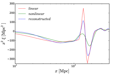
Figure 1: The linear (dashed line), nonlinear (solid line), and reconstructed (dotted line) correlation functions. The distortion of the BAO peak is reduced by reconstruction.

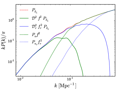
Figure 2: The linear power spectrum (dashed line), the linear parts of the nonlinear (thick solid line) and reconstructed (thin solid line) power spectra, the noise parts of the nonlinear (thick dotted line) and reconstructed (thin dotted line) power spectra. For visual comparisions, we rescale both the linear and noise parts by $f^{2}=P_{\delta_{L}}/P_{\delta}$ and $f^{2}_{r}=P_{\delta_{L}}/P_{\delta_{r}}$ for the nonlinear and reconstructed fields, respectively. The noise terms dominate over the signals at $k\gtrsim 0.07\ \mathrm{Mpc}^{-1}$ for the nonlinear field and $k_{q}\gtrsim 0.24\ \mathrm{Mpc}^{-1}$ for the reconstructed field.

To conveniently quantify the linear information $\delta_{L}$ in the nonlinear density field $\delta$, we decompose the nonlinear density field $\delta$ as

$$\delta({k})=b({k})\delta_{L}({k})+n({k}).$$ (6)

Here, $b\delta_{L}$ is completely correlated with the linear density field $\delta_{L}$. Correlating the nonlinear density field with the linear density field,

$$\langle\delta(k)\delta_{L}(k)\rangle=b(k)\langle\delta_{L}(k)\delta_{L}(k)\rangle,$$ (7)

we obtain

$$b(k)=\frac{P_{\delta\delta_{L}}(k)}{P_{\delta_{L}}(k)}.$$ (8)

Nonlinear evolution drives $b(k)$ to drop from unity, reducing the linear signal. Separating the part correlated with the linear density field, we have $n(k)=\delta(k)-b(k)\delta_{L}(k)$. $n(k)$ is generated in the nonlinear evolution and thus uncorrelated with the linear density field $\delta_{L}$, further reducing $b\delta_{L}$ with respect to $\delta$. This part induces noise in the measurement of BAO. Such decomposition helps to write the nonlinear power spectrum as

$$P_{\delta}(k)=\mathcal{D}(k)P_{\delta_{L}}(k)+P_{n}(k),$$ (9)

where $\mathcal{D}(k)=b^{2}(k)$ is the nonlinear damping factor. Here, $b(k)$ is often referred as the “propagator” and $P_{n}$ is usually called the “mode-coupling” term Crocce and Scoccimarro (2006, 2008); Matsubara (2008). For the reconstructed field $\delta_{r}(q)$, we also have

$$\delta_{r}(k_{q})=b_{r}(k_{q})\delta_{L}(k_{q})+n_{r}(k_{q}),$$ (10)

where $b_{r}(k_{q})={P_{\delta_{r}\delta_{L}}(k_{q})}/{P_{\delta_{L}}(k_{q})}$. Similarly, the reconstructed power spectrum is given by

$$P_{\delta_{r}}(k)=\mathcal{D}_{r}(k)P_{\delta_{L}}(k)+P_{n_{r}}(k),$$ (11)

where $\mathcal{D}_{r}(k)=b^{2}_{r}(k)$. Here, the subscript “$q$” denotes that the reconstructed field is given on the Lagrangian coordinate. In Fig. 2, we plot the linear components and the noise terms of the nonlinear and reconstructed fields.

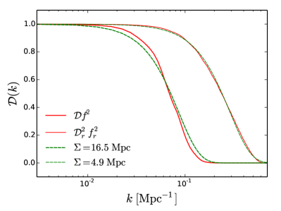
Figure 3: The damping factors for the nonlinear (thick solid line) and reconstructed (thin solid line) fields. The Gaussian BAO damping models with $\Sigma=16.5\ \mathrm{Mpc}$ (thick dashed line) and $\Sigma=4.9\ \mathrm{Mpc}$ (thin dashed line).

Figure 3 shows the damping factors for the nonlinear and reconstructed fields. The damping of the linear power spectrum is significantly reduced after reconstruction. We also overplot the best-fitting Gaussian BAO damping model,

$$\mathcal{D}(k)=\mathrm{e}^{-k^{2}\Sigma^{2}/2},$$ (12)

with $\Sigma=16.5\ \mathrm{Mpc}$ and $4.9\ \mathrm{Mpc}$ for the nonlinear and reconstructed fields. The new BAO reconstruction algorithm reduces the nonlinear damping scale $\Sigma$ by 70 percent. The damping factor for the reconstructed field is above $0.9$ for $k\lesssim 0.1\ \mathrm{Mpc}^{-1}$. However, the 100 percent reconstruction, cancelling any nonlinear effects, is still unachievable, as some information has been irreversibly lost.

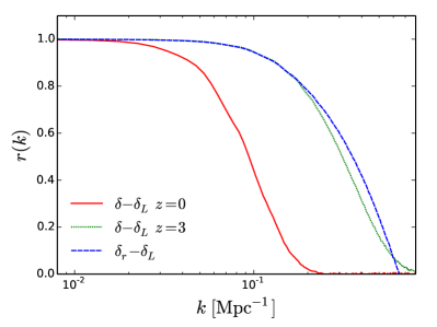
Figure 4: The $\delta-\delta_{L}$ correlation coefficients at $z=0$ (solid line) and $z=3$ (dotted line), as well as the $\delta_{r}-\delta_{L}$ correlation coefficient (dashed line).

Reconstruction reduces the nonlinear damping $\mathcal{D}(k)$ as well as the noise term $P_{n}(k)$. To quantify the overall performance, we can use the cross-correlation coefficient

$$r(k)=\frac{P_{\delta\delta_{L}}(k)}{\sqrt{P_{\delta}(k)P_{\delta_{L}}(k)}}=\frac{1}{\sqrt{1+\eta(k)}},$$ (13)

where $\eta=P_{n}/(b^{2}P_{\delta_{L}})$ quantifies the relative amplitude of $n$ with respect to $b\delta_{L}$. We plot the cross-correlation coefficients in Fig. 4. The correlation of $\delta_{r}$ with $\delta_{L}$ is even better than that of $\delta$ at $z=3$.

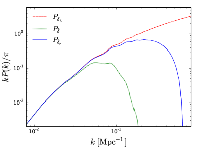
Figure 5: The power spectra for the linear (dashed line), filtered nonlinear (dotted line) and filtered reconstructed (solid line) fields. The wiggles in the reconstructed power spectrum are much more apparent than the nonlinear power spectrum.

The raw reconstructed field $\delta_{r}$ is still noisy on small scales ($k_{q}\gtrsim 0.24\ \mathrm{Mpc}^{-1}$). To optimally filter out the noise from the raw reconstructed field, we use the Wiener filter

$$W_{r}(k_{q})=\frac{P_{\delta_{L}}(k_{q})}{P_{\delta_{L}}(k_{q})+P_{n_{r}}(k_{q})/b_{r}^{2}(k_{q})}.$$ (14)

Deconvolving $b_{r}$ and using the Wiener filter, we obtain the optimal reconstructed field,

$$\tilde{\delta}_{r}(k_{q})=\frac{\delta_{r}(k_{q})}{b_{r}(k_{q})}W_{r}(k_{q}).$$ (15)

The power spectrum of the optimal reconstructed field $\tilde{\delta}_{r}$ is given by

$$P_{\tilde{\delta}_{r}}(k_{q})=W_{r}^{2}(k_{q})P_{\delta_{L}}(k_{q})+W_{r}^{2}(k_{q}){P_{n_{r}}(k_{q})}/{b_{r}^{2}(k_{q})}.$$ (16)

The raw nonlinear field $\delta$ is also filtered. In Fig. 5, we plot the power spectra of the optimal filtered reconstructed and nonlinear fields. The wiggles in the reconstructed power spectrum are much more apparent than the nonlinear power spectrum.

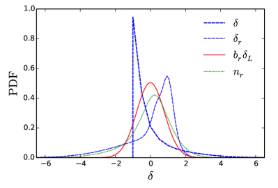
Figure 6: The probability distribution functions of the nonlinear (thick dashed line) and reconstructed (thin dashed line) fields. We also show the PDFs of the linear component (solid line) and the noise part (dotted line). The PDFs are evaluated on $N_{\mathrm{grid}}=6\times 10^{7}$ grids, i.e., the grid scale is $5/3\ \mathrm{Mpc}$.

The density fluctuation probability distribution function (PDF) quantifies the Gaussianity of the density field. Figure 6 shows the PDFs of the nonlinear and reconstructed density fields. We also plot the PDFs of the linear component $b_{r}\delta_{L}$ and the noise part $n_{r}$ of the reconstructed density field $\delta_{r}$. Of course the linear component is Gaussian, while the noise part is nonGaussian. As a result, the reconstructed density field is also nonGaussian. The raw nonlinear density field is clearly nonGaussian.

V Discussions

The new reconstruction method successfully recovers the lost linear information on the mildly nonlinear scales (till $k\lesssim 0.24\ \mathrm{Mpc}^{-1}$). The result in 1D provides an intuitive view of the algorithm and motivates us to develop the reconstruction method in 3D. The nonlinear displacement beyond the Zel’dovich approximation in 3D can be solved using the multigrid iteration scheme Pen (1995). The algorithm for solving the 3D nonlinear displacement is originally introduced for the adaptive particle-mesh $N$-body code Pen (1995) and the moving mesh hydrodynamic code Pen (1998). The 3D case is also more complicated since the 3D displacement field involves a curl part (vorticity) which is generated after shell crossing, while this does not happen after particles cross over in 1D. This requires us to quantify the effect of vorticity, which can be accomplished using $N$-body simulations. By decomposing the simulated displacement field into a irrotational part and a curl part, we can study the statistical properties of different components Zhang et al. (2013); Zheng et al. (2013). These will be presented in future.

The reconstructed nonlinear displacement field is also important for the current BAO reconstruction Eisenstein et al. (2007), where the linear continuity equation is adopted to solve the displacement under the Zel’dovich approximation. However, the nonlinear displacement retains much more information, describing the motion of dark matter fluid elements beyond the linear order. The reconstructed displacement field $s(q)$ is given on the Lagrangian coordinate instead of the final Eulerian coordinate. This helps to correct the effect due to the use of $s(x)$ instead of $s(q)$ in the BAO reconstruction White (2015); Schmittfull et al. (2015). As more nonlinear effects will be removed using the nonlinear displacement, we expect the modeling of the reconstructed density field will be simplified.

The Wiener filter is optimal for the case both the signal and the noise are Gaussian random fields. In Fig. 6, the PDFs of the reconstructed density field and the noise are apparently nonGaussian. The reconstruction can be further improved using the nonlinear filter rather than the Wiener filter Pen (1999). We plan to study this in future.

VI Acknowledgements

We are very grateful to Matthew McQuinn for providing the 1D $N$-body simulations and helpful comments on the manuscript. We also thank Yu Yu, Tian-Xiang Mao and Wen-Xiao Xu for useful discussions. We acknowledge the support of the Chinese MoST 863 program under Grant No. 2012AA121701, the CAS Science Strategic Priority Research Program XDB09000000, the NSFC under Grant No. 11373030, IAS at Tsinghua University, and NSERC. The Dunlap Institute is funded through an endowment established by the David Dunlap family and the University of Toronto. Research at the Perimeter Institute is supported by the Government of Canada through Industry Canada and by the Province of Ontario through the Ministry of Research $\&$ Innovation.

References

- McQuinn and White (2016) M. McQuinn and M. White, J. Cosmology Astropart. Phys 1, 043 (2016), eprint 1502.07389.
- Eisenstein et al. (2007) D. J. Eisenstein, H.-J. Seo, E. Sirko, and D. N. Spergel, ApJ 664, 675 (2007), eprint astro-ph/0604362.
- Schmittfull et al. (2015) M. Schmittfull, Y. Feng, F. Beutler, B. Sherwin, and M. Y. Chu, Phys. Rev. D 92, 123522 (2015), eprint 1508.06972.
- Crocce and Scoccimarro (2006) M. Crocce and R. Scoccimarro, Phys. Rev. D 73, 063520 (2006), eprint astro-ph/0509419.
- Crocce and Scoccimarro (2008) M. Crocce and R. Scoccimarro, Phys. Rev. D 77, 023533 (2008), eprint 0704.2783.
- Matsubara (2008) T. Matsubara, Phys. Rev. D 77, 063530 (2008), eprint 0711.2521.
- Pen (1995) U.-L. Pen, ApJS 100, 269 (1995).
- Pen (1998) U.-L. Pen, ApJS 115, 19 (1998), eprint astro-ph/9704258.
- Zhang et al. (2013) P. Zhang, J. Pan, and Y. Zheng, Phys. Rev. D 87, 063526 (2013), eprint 1207.2722.
- Zheng et al. (2013) Y. Zheng, P. Zhang, Y. Jing, W. Lin, and J. Pan, Phys. Rev. D 88, 103510 (2013), eprint 1308.0886.
- White (2015) M. White, MNRAS 450, 3822 (2015), eprint 1504.03677.
- Pen (1999) U.-L. Pen, Philosophical Transactions of the Royal Society of London Series A 357, 2561 (1999), eprint astro-ph/9904170.