Spin effects in the pion holographic light-front wavefunction

Abstract

We account for dynamical spin effects in the holographic light-front wavefunction of the pion in order to predict the mean charge radius, $\sqrt{\langle r^{2}_{\pi}\rangle}$, the decay constant, $f_{\pi}$, the spacelike electromagnetic form factor, $F_{\pi}(Q^{2})$, the twist-$2$ pion Distribution Amplitude and the photon-to-pion transition form factor $F_{\gamma\pi}(Q^{2})$. Using a universal fundamental AdS/QCD scale, $\kappa=523$ MeV, and a constituent quark mass of $330$ MeV, we find a remarkable improvement in describing all observables.

I Introduction

Hadronic light-front wavefunctions (LFWFs) provide the underlying link between the fundamental degrees of freedom of QCD, i.e. quarks and gluons, and their asymptotic hadronic states. LFWFs thus encode both the physics of confinement and chiral symmetry breaking, which are fundamental, intimately related Horn and Roberts (2016) and yet not fully understood, emergent properties of QCD. In phenomenology, LFWFs are extremely important since all hadronic properties can, in principle, be derived from them. For example, in the exclusive decays of the $B$ meson to light mesons, which are under intense investigation at the LHCb experiment, the theoretical non-perturbative inputs, i.e. the meson decay constants, Distribution Amplitudes and transition form factors can all be computed if the LFWFs of the mesons are known. These non-perturbative inputs are in fact the major source of theoretical uncertainties in current Standard Model predictions Ali (2016).

In principle, LFWFs are obtained by solving the LF Heisenberg equation for QCD: Brodsky et al. (2015)

$$H_{\text{QCD}}^{\text{LF}}|\Psi(P)\rangle=M^{2}|\Psi(P)\rangle$$ (1)

where $H_{\text{QCD}}^{\text{LF}}=P^{+}P^{-}-P_{\perp}^{2}$ is the LF QCD Hamiltonian and $M$ is the hadron mass. At equal light-front time $(x^{+}=0)$ and in the light-front gauge $A^{+}=0$, the hadron state $|\Psi(P)\rangle$ admits a Fock expansion, i.e.

$$|\Psi(P^{+},\mathbf{P_{\perp}},S_{z})\rangle=\sum_{n,h_{i}}\int[\mathrm{d}x_{i}][\mathrm{d}^{2}\mathbf{k}_{\perp i}]\frac{1}{\sqrt{x_{i}}}\Psi_{n}(x_{i},\mathbf{k}_{\perp i},h_{i})|n:x_{i}P^{+},x_{i}\mathbf{P_{\perp}}+\mathbf{k}_{\perp i},h_{i}\rangle$$ (2)

where $\Psi_{n}(x_{i},\mathbf{k}_{\perp i},h_{i})$ is the LFWF of the Fock state with $n$ constituents and the integration measures are given by

$$[\mathrm{d}x_{i}]\equiv\prod_{i}^{n}\mathrm{d}x_{i}\delta(1-\sum_{j=1}^{n}x_{j})\hskip 28.45274pt[\mathrm{d}^{2}\mathbf{k}_{i}]\equiv\prod_{i=1}^{n}\frac{\mathrm{d}^{2}\mathbf{k}_{i}}{2(2\pi)^{3}}16\pi^{3}\delta^{2}(\sum_{j=1}^{n}\mathbf{k}_{i})\;.$$ (3)

LFWFs are quantum mechanical probability amplitudes that depends on the momenta fraction $x_{i}=k_{i}^{+}/P^{+}$, the transverse momenta $\mathbf{k}_{\perp i}$, and the helicities $h_{i}$ of the constituents. In practice, it is difficult, if not impossible, to solve Eq. (1) since it contains an infinite number of strongly coupled integral equations. Various approximation schemes involve truncating the Fock expansion, using discretized light-front quantization or solving the equations in a lower number of spatial dimensions. For a review of light-front quantum field theories, we refer to Brodsky et al. (1998).

A remarkable breakthrough during the last decade is the discovery by Brodsky and de Téramond de Teramond and Brodsky (2009); Brodsky and de Teramond (2006); de Teramond and Brodsky (2005); Brodsky and de Teramond (2008a) of a higher dimensional gravity dual to a semiclassical approximation of light-front QCD. The result is a relativistic Schrödinger-like wave equation for mesons that can be solved analytically to predict meson spectroscopy and LFWFs in terms of a single mass scale $\kappa$. The approach can also include baryons de Teramond and Brodsky (2005) and more recently has been extended to a unified framework for baryons and mesons considered as conformal superpartners Brodsky et al. (2016). This gauge/gravity duality is referred to as light-front holography (LFH) and is reviewed in Ref. Brodsky et al. (2015).

In the semiclassical approximation, quark masses and quantum loops are neglected, the LFWFs depend on the invariant mass $\mathcal{M}^{2}=(\sum_{i}^{n}k_{i})^{2}$ of the constituents rather than on their individual momenta $k_{i}$. For the valence ($n=2$ for mesons) Fock state, the invariant mass of the $q\bar{q}$ pair is $\mathcal{M}_{q\bar{q}}^{2}=k_{\perp}^{2}/x(1-x)$ and the latter is the Fourier conjugate to the impact variable $\zeta^{2}=x(1-x)b^{2}$ where $b$ is the transverse separation the quark and antiquark. The valence meson LFWF can then be written in a factorized form:

$$\Psi(\zeta,x,\phi)=e^{iL\phi}\mathcal{X}(x)\frac{\phi(\zeta)}{\sqrt{2\pi\zeta}}$$ (4)

where the helicity indices have been suppressed Brodsky et al. (2015). We note that this suppression of the helicity indices is legitimate if either the constituents are assumed to be spinless or if the helicity dependence decouples from the dynamics. It can then be shown that Eq. (1) reduces to a $1$-dimensional Schrödinger-like wave equation for the transverse mode of LFWF of the valence ($n=2$ for mesons) state, namely:

$$\left(-\frac{d^{2}}{d\zeta^{2}}-\frac{1-4L^{2}}{4\zeta^{2}}+U(\zeta)\right)\phi(\zeta)=M^{2}\phi(\zeta)$$ (5)

where all the interaction terms and the effects of higher Fock states on the valence state are hidden in the confinement potential $U(\zeta)$. The latter remains to be specified and, at present, this cannot be done from first principles in QCD.

However, Brodsky and de Téramond found that Eq. (5) maps onto the wave equation for the propagation of spin-$J$ string modes in the higher dimensional anti-de Sitter space, $\text{AdS}_{5}$, if the impact light-front variable $\zeta$ is identified with $z_{5}$, the fifth dimension of AdS space and the light-front orbital angular momentum $L^{2}$ is mapped onto $(mR)^{2}-(2-J)^{2}$ where $R$ and $m$ are the AdS radius and mass respectively. For this reason, we refer to Eq. (5) as the holographic LF Schrödinger equation. In this AdS/QCD duality, the confining potential in physical spacetime is driven by the deformation of the pure $\text{AdS}_{5}$ geometry. Specifically, the potential is given by

$$U(z_{5},J)=\frac{1}{2}\varphi^{\prime\prime}(z_{5})+\frac{1}{4}\varphi^{\prime}(z_{5})^{2}+\left(\frac{2J-3}{4z_{5}}\right)\varphi^{\prime}(z_{5})$$ (6)

where $\varphi(z_{5})$ is the dilaton field which breaks conformal invariance in AdS space. A quadratic dilaton, $\varphi(z_{5})=\kappa^{2}z_{5}^{2}$, profile results in a light-front harmonic oscillator potential in physical spacetime:

$$U(\zeta,J)=\kappa^{4}\zeta^{2}+\kappa^{2}(J-1)$$ (7)

since $z_{5}$ maps onto the LF impact variable $\zeta$. Remarkably, Brodsky, Dosch and de Téramond have shown that the quadratic form of the AdS/QCD potential is unique Brodsky et al. (2014). In fact, starting with a more general dilaton profile $\varphi\propto z_{5}^{s}$ and requiring the pion to be massless, uniquely fixes $s=2$ Brodsky et al. (2013). More formally, applying the mechanism of de Alfaro, Furbini and Furlan de Alfaro et al. (1976) (which allows the emergence of a mass scale in the Hamiltonian of a conformal $1$-dimensional QFT while retaining the conformal invariance of the underlying action) to semiclassical LF QCD uniquely fixes the quadratic form of the AdS/QCD potential Brodsky et al. (2014).

With the confining potential specified, one can solve the holographic Schrödinger equation to obtain the meson mass spectrum,

$$M^{2}=4\kappa^{2}\left(n+L+\frac{S}{2}\right)\;$$ (8)

which, as expected, predicts a massless pion. The corresponding normalized eigenfunctions are given by

$$\phi_{nL}(\zeta)=\kappa^{1+L}\sqrt{\frac{2n!}{(n+L)!}}\zeta^{1/2+L}\exp{\left(\frac{-\kappa^{2}\zeta^{2}}{2}\right)}L_{n}^{L}(x^{2}\zeta^{2})\;.$$ (9)

To completely specify the holographic meson wavefunction, we need the analytic form of the longitudinal mode $\mathcal{X}(x)$. This is obtained by matching the expressions for the pion EM or gravitational form factor in physical spacetime and in AdS space. Either matching consistently results in $\mathcal{X}(x)=\sqrt{x(1-x)}$ de Teramond and Brodsky (2009); Brodsky and de Teramond (2008b). The meson holographic LFWFs for massless quarks can thus be written in closed form:

$$\Psi_{nL}(\zeta,x,\phi)=e^{iL\phi}\sqrt{x(1-x)}(2\pi)^{-1/2}\kappa^{1+L}\sqrt{\frac{2n!}{(n+L)!}}\zeta^{L}\exp{\left(\frac{-\kappa^{2}\zeta^{2}}{2}\right)}L_{n}^{L}(x^{2}\zeta^{2})$$ (10)

with the corresponding meson masses lying on linear Regge trajectories as given by Eq. (8). The reasons why a solution to a quantum field theory could reduce to a solution of a simple, one-dimensional differential equation are explored in Ref. Glazek and Trawiński (2013).

For phenomenological applications, it is necessary to restore both the quark mass and helicity dependence of the holographic LFWF. In fact, it has recently been shown in Ref. Swarnkar and Chakrabarti (2015) that non-zero light quark masses drastically improves the description of data on the photon-to-pion, photon-to-$\eta$ and photon-to-$\eta^{\prime}$ transition form factors. On the other hand, for the pion and kaon EM form factors, the description of data actually worsens unless $3$ data points at large $Q^{2}$ are excluded for the kaon form factor Swarnkar and Chakrabarti (2015). Accounting for non-zero light quark masses means going beyond the semiclassical approximation, and this is usually done following the prescription of Brodsky and de Téramond Brodsky and de Teramond (2009). For the ground state pion, this leads to

$$\Psi^{\pi}(x,\zeta^{2})=\mathcal{N}\sqrt{x(1-x)}\exp{\left[-{\kappa^{2}\zeta^{2}\over 2}\right]}\exp{\left[-{m_{f}^{2}\over 2\kappa^{2}x(1-x)}\right]}$$ (11)

where $\mathcal{N}$ is a normalization constant fixed by requiring that

$$\int\mathrm{d}^{2}\mathbf{b}\mathrm{d}x|\Psi^{\pi}(x,\zeta^{2})|^{2}=P_{q\bar{q}}$$ (12)

where $P_{q\bar{q}}$ is the probability that the meson consists of the leading quark-antiquark Fock state.

Note that Eq. (8) tells us that the AdS/QCD scale $\kappa$ can be chosen to fit the experimentally measured Regge slopes. Ref. Brodsky et al. (2015) reports $\kappa=590$ MeV for pseudoscalar mesons and $\kappa=540$ MeV for vector mesons. A recent fit to the Regge slopes of mesons and baryons, treated as conformal superpartners, yields $\kappa=523$ MeV Brodsky et al. (2016). On the other hand, the AdS/QCD scale $\kappa$ can be connected to the scheme-dependent pQCD renormalization scale $\Lambda_{\text{QCD}}$ by matching the running strong coupling in the non-perturbative (described by light-front holography) and the perturbative regimes Brodsky et al. (2010). With $\kappa=523$ MeV and the $\beta$-function of the QCD running coupling at $5$-loops, Brodsky, Deur and de Téramond recently predicted the QCD renormalization scale, $\Lambda^{{\overline{MS}}}_{\text{QCD}}$, in excellent agreement with the world average value Deur et al. (2016). Furthermore, light-front holographic wavefunctions have also been used to predict diffractive vector meson productionForshaw and Sandapen (2012); Ahmady et al. (2016). A fit to the HERA data on diffractive $\rho$ electroproduction, with $m_{u/d}=140$ MeV, gives $\kappa=560$ MeVForshaw and Sandapen (2012) and using $\kappa=550$ MeV (with $m_{u/d}[m_{s}]=46[140]$ MeV) leads to a good simultaneous description of the HERA data on diffractive $\rho$ and $\phi$ electroproduction Ahmady et al. (2016). These findings hint towards the emergence of a universal fundamental AdS/QCD scale $\kappa\sim 550$ MeV. In the most recent application of LFH to predict nucleon EM form factors Sufian et al. (2016), it is pointed out that this universality holds up to $10\%$ accuracy. In this paper, we shall use the value of $\kappa=523$ MeV which fits the meson/baryon Regge slopes and accurately predicts $\Lambda^{{\overline{MS}}}_{\text{QCD}}$ Brodsky et al. (2016); Deur et al. (2016).

In earlier applications of LFH with massless quarks, much lower values of $\kappa$ were required to fit the pion data: $\kappa=375$ MeV in Ref. Brodsky and de Teramond (2008a) in order to fit the pion EM form factor data and $\kappa=432$ MeV (with $P_{q\bar{q}}=0.5$) to fit the photon-to-pion transition form factor data simultaneously at large $Q^{2}$ and $Q^{2}=0$ (the latter is fixed by the $\pi^{0}\to\gamma\gamma$ decay width) Brodsky et al. (2011a). Note that in Ref. Brodsky and de Teramond (2008a), the EM form factor is computed, both in the spacelike and timelike regions, as a convolution of normalizable hadronic modes with a non-normalizable EM current which propagates in the modified infrared region of AdS space and generates the non-perturbative pole structure of the EM form factor in the timelike region. Alternatively, the spacelike EM form factor can be computed using the Drell-Yan-West formula Drell and Yan (1970); West (1970) in physical spacetime with the holographic pion LFWF. The latter approach is taken in Refs. Vega and Schmidt (2009); Swarnkar and Chakrabarti (2015); Vega et al. (2009); Branz et al. (2010). In Ref. Vega et al. (2009), a higher value of $\kappa=787$ MeV is used with $m_{u/d}=330$ MeV and the authors predict $P_{q\bar{q}}=0.279$, implying an important contribution of higher Fock states in the pion. In Ref. Branz et al. (2010), a universal AdS/QCD scale $\kappa=550$ MeV is used for all mesons, together with a constituent quark mass $m_{u/d}=420$ MeV, but $P_{q\bar{q}}=0.6$ is fixed for the pion only: for the kaon, $P_{q\bar{q}}=0.8$ and for all other mesons, $P_{q\bar{q}}=1$. More recently, in Ref. Swarnkar and Chakrabarti (2015), with $m_{u/d}=330$ MeV, the authors use a universal $\kappa=550$ MeV for all mesons but fix the wavefunction normalization for the pion so as to fit the decay constant. Consequently, this implies that $P_{q\bar{q}}=0.61$ only for the pion.

All these previous studies seem to indicate that a special treatment is required at least for the pion either by using a distinct AdS/QCD scale $\kappa$ or/and relaxing the normalization condition on the holographic wavefunction, i.e. invoking higher Fock states contributions. This may well be reasonable since the pion is indeed unnaturally light and does not lie on a Regge trajectory, as pointed out in Ref. Vega and Schmidt (2009). However, we note that in the previous studies Swarnkar and Chakrabarti (2015); Vega et al. (2009); Branz et al. (2010) where the pion observables are predicted using the holographic wavefunction, given by Eq. (11), the helicity dependence of the latter is always assumed to decouple from the dynamics, i.e. the helicity wavefunction is taken to be momentum-independent. This is actually consistent with the semi-classical approximation within which the AdS/QCD correspondence is exact. Consequently, Ref. Branz et al. (2010) derives a single formula to predict simultaneously the vector and pseudoscalar meson decay constants, so that using a universal scale $\kappa$ and $P_{q\bar{q}}=1$ for all mesons inevitably leads to degenerate decay constants in conflict with experiment.

In this paper, we show that it is possible to achieve a better description of the pion observables by using a universal AdS/QCD scale $\kappa$ and without the need to invoke higher Fock state contributions. We do so by taking into account dynamical spin effects in the holographic pion wavefunction, i.e. we use a momentum-dependent helicity wavefunction. This approach goes beyond the semiclassical approximation, just like the inclusion of light quark masses in the holographic wavefunction. However, it does support the idea of the emergence of a universal, fundamental AdS/QCD scale. A similar approach was taken previously for the $\rho$ meson, leading to impressive agreement to the HERA data on diffractive $\rho$ electroproduction Forshaw and Sandapen (2012).

II Dynamical spin effects

To restore the helicity dependence of the holographic wavefunction, we assume that

$$\Psi(x,\mathbf{k})\to\Psi_{h\bar{h}}(x,\mathbf{k})=S_{h\bar{h}}(x,\mathbf{k})\Psi(x,\mathbf{k})$$ (13)

where $S_{h\bar{h}}(x,\mathbf{k})$ corresponds to the helicity wavefunction for a point-like meson-$q\bar{q}$ coupling. For vector mesons, the helicity wavefunction is therefore similar to that of the point-like photon-$q\bar{q}$ coupling, i.e.

$$S_{h\bar{h}}^{V}(x,\mathbf{k})=\frac{\bar{v}_{\bar{h}}((1-x)P^{+},-\mathbf{k})}{\sqrt{(1-x)}}[\gamma\cdot\epsilon_{V}]\frac{u_{h}(xP^{+},\mathbf{k})}{\sqrt{x}}$$ (14)

where $\epsilon_{V}^{\mu}$ is the polarization vector of the vector meson. Indeed, substituting $\epsilon_{V}^{\mu}$ by the photon polarization vector and multiplying Eq. (14) by the light-front energy denominator Lepage and Brodsky (1980) yields the well-known photon light-front wavefunctions Lepage and Brodsky (1980); Dosch et al. (1997); Kulzinger et al. (1999); Nemchik et al. (1997); Forshaw et al. (2004). This assumption for the helicity structure of the vector meson is very common when computing diffractive vector meson production in the dipole model Nemchik et al. (1997); Forshaw et al. (2004); Watt and Kowalski (2008); Forshaw et al. (2006); Forshaw and Sandapen (2010, 2011); Armesto and Rezaeian (2014); Rezaeian and Schmidt (2013); Goncalves et al. (2016); Rezaeian et al. (2013) and, as we mentioned earlier, was used in Ref. Forshaw and Sandapen (2012) with the holographic wavefunction for the $\rho$ meson.

For the pseudoscalar pion, we replace $\gamma\cdot\epsilon_{V}$ in Eq. (14) by $(\mbox{scalar function})\times\gamma^{5}$ where the most general, dimensionally homogeneous, scalar function that can be constructed using the pion’s momentum is $A(P\cdot\gamma)+B\sqrt{P\cdot P}$ with $A$ and $B$ being arbitrary constants. Hence

$$S^{\pi}_{h\bar{h}}(x,\mathbf{k})=\frac{\bar{v}_{\bar{h}}((1-x)P^{+},-\mathbf{k})}{\sqrt{1-x}}\left[(A\not{P}+BM_{\pi})\gamma^{5}\right]\frac{u_{h}(xP^{+},\mathbf{k})}{\sqrt{x}}\;.$$ (15)

We note that References Heinzl (2001, 2000) take $A=B=1$, quoting Dziembowski (1988); Jaus (1990); Ji and Cotanch (1990); Ji et al. (1992). References Choi and Ji (2007); Trawiński (2016) take $A=0$ and the recent paper Chang et al. (2016) considers $A=B=1$ but retains only the $\gamma^{+}\gamma^{5}$ term in the scalar product $\not{P}\gamma^{5}$. This implies a momentum-independent (non-dynamical) helicity wavefunction if $B=0$ and that dynamical spin effects are only allowed if $B\neq 0$. After evaluating the right-hand-side using the light-front spinors given in Ref. Lepage and Brodsky (1980), we obtain

$$S_{h\bar{h}}^{\pi}(x,\mathbf{k})=\left\{AM_{\pi}^{2}+B\left(\frac{m_{f}M_{\pi}}{x(1-x)}\right)\right\}(2h)\delta_{-h\bar{h}}+B\left(\frac{M_{\pi}ke^{i(2h)\theta_{k}}}{x(1-x)}\right)\delta_{h\bar{h}}$$ (16)

with $\mathbf{k}=ke^{i\theta_{k}}$. As mentioned above, if we take $B=0$, the helicity wavefunction becomes momentum-independent:

$$S^{\pi}_{h\bar{h}}(x,\mathbf{k})\to S^{\pi}_{h\bar{h}}=\frac{1}{\sqrt{2}}(2h)\delta_{-h\bar{h}}$$ (17)

normalized such that $\sum_{h\bar{h}}|S^{\pi}_{h,\bar{h}}|^{2}=1$. Such a helicity wavefunction is assumed for the meson (both pseudoscalar and vector) holographic wavefunction in Refs. Swarnkar and Chakrabarti (2015); Vega et al. (2009) and we shall refer to it as the non-dynamical (i.e. momentum-independent) helicity wavefunction, consistent with the semi-classical approximation of light-front holography. Our spin-improved helicity wavefunction allows for an additional momentum-dependent contribution in the opposite-helicities part of the wavefunction as well as configurations in which the quark and antiquark have same helicities Leutwyler (1974a, b). Note that the same-helicities terms are eigenfunctions of the LF orbital angular momentum operator given by Brodsky et al. (2015)

$$L_{z}=-i\left(k_{y}\partial_{k_{x}}-k_{x}\partial_{k_{y}}\right)=i\partial_{\theta_{k}}$$ (18)

with eigenvalues $L_{z}=-2h$. In other words, for this same-helicities component of our pion wavefunction, the orbital angular momentum $L_{z}=-S_{z}$ where $S_{z}=h+\bar{h}=2h$ so that $J_{z}=L_{z}+S_{z}=0$ as required for the pion. Note that when we allow for dynamical spin effects, we are going beyond the semi-classical approximation, and Eq. (8) needs to modified due to a spin-orbit interaction term (not specified in this paper) in the light-front Schödinger equation. It is also useful to check that our spin-improved wavefunction transforms correctly under the LF parity operator, $\mathcal{P}_{\perp}$, which flips the signs of all helicities and that of the $x$ (or $y$) component of the transverse momentum: Brodsky et al. (2006)

$$\Psi^{\pi}_{h\bar{h}}(x,\mathbf{k})\xrightarrow{\mathcal{P}_{\perp}}\Psi^{\pi}_{-h,-\bar{h}}(x,\tilde{\mathbf{k}})$$ (19)

where $\tilde{\mathbf{k}}=-k_{x}+ik_{y}=ke^{i(\pi-\theta_{k})}$. Since $e^{-i2h(\pi-\theta_{k})}=-e^{i2h\theta_{k}}$, it is explicit from Eq. (16), that our spin-improved wavefunction is parity-odd, i.e.

$$\mathcal{P}_{\perp}\Psi^{\pi}_{h,\bar{h}}(x,\mathbf{k})=-\Psi^{\pi}_{h,\bar{h}}(x,\mathbf{k})$$ (20)

as required for the pion.

A two-dimensional Fourier transform of our spin-improved wavefunction to impact space gives

$$\Psi^{\pi}_{h\bar{h}}(x,\mathbf{b})=\{(Ax(1-x)M_{\pi}^{2}+Bm_{f}M_{\pi})(2h)\delta_{-h\bar{h}}-BM_{\pi}i\partial_{b}\delta_{h\bar{h}}\}\frac{\Psi^{\pi}(x,\zeta^{2})}{x(1-x)}$$ (21)

which can be compared to the original holographic wavefunction,

$$\Psi^{\pi[\text{o}]}_{h\bar{h}}(x,\mathbf{b})=\frac{1}{\sqrt{2}}h\delta_{-h\bar{h}}\Psi^{\pi}(x,\zeta^{2})$$ (22)

where $\Psi^{\pi}(x,\zeta^{2})$ in both of the above equations, is the holographic wavefunction given by Eq. (11). We now fix the normalization constant $\mathcal{N}$ appearing in Eq. (11) by requiring that

$$\int\mathrm{d}^{2}\mathbf{b}\mathrm{d}x|\Psi^{\pi}(x,\mathbf{b})|^{2}=1$$ (23)

where

$$|\Psi^{\pi}(x,\mathbf{b})|^{2}\equiv\sum_{h,\bar{h}}|\Psi^{\pi}_{h\bar{h}}(x,\mathbf{b})|^{2}\;.$$ (24)

Note that Eq. (23) reduces to the normalization condition given by Eq. (12) (with $P_{q\bar{q}}=1$) if we substitute the original holographic wavefunction, Eq. (22), in Eq. (23). Imposing our normalization condition, Eq. (23), implies that we assume that the pion consists only of the leading quark-antiquark Fock state.

In Figure 1, we show the dynamical spin effects in the squared and helicity-summed holographic wavefunction with a constituent quark mass, $m_{u/d}=330$ MeV. Recall that we recover the original holographic pion wavefunction by taking $B=0$ in our spin-improved wavefunction. In addition, we consider the two cases $[A=0,B=1]$ and $[A=1,B=1]$ that allow for dynamical spin effects. It can be seen that, at fixed $x=0.5$ (and $x=0.1$), the spin-improved wavefunctions are suppressed (and enhanced) respectively, compared to the original wavefunction. At fixed $b=0$ and $b=5~{}\mbox{GeV}^{-1}$, the spin-improved wavefunctions are broader than the original wavefunction. In Figure 2, we compare the $3$-dimensional plots of the spin-improved wavefunctions to the original wavefunction, which clearly show that dynamical spin effects enhance the end-point contributions in $x$.

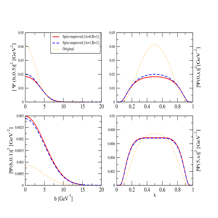
Figure 1: The pion holographic LFWF squared and summed over all helicities: $|\Psi^{\pi}(x,\mathbf{b})|^{2}~{}[\text{GeV}^{2}]$. Dotted-orange: original. Continous-red: spin-improved ($A=0,B=1$). Dashed-blue: spin-improved ($A=1,B=1$ ). Left: The $b$-dependence of the wavefunction at fixed $x=0.5$ (upper) and $x=0.1$ (lower). Right: The $x$-dependence of the wavefunction at fixed $b=0$ (upper) and $b=5~{}\text{GeV}^{-1}$ (lower). All plots are generated with $\kappa=523$ MeV and $m_{u/d}=330$ MeV.

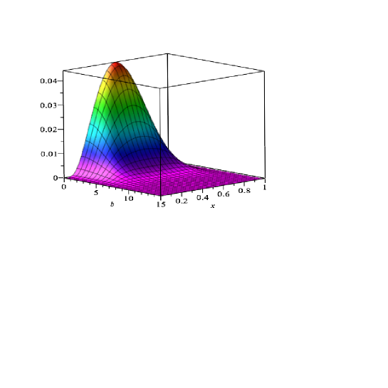
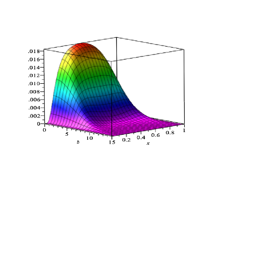
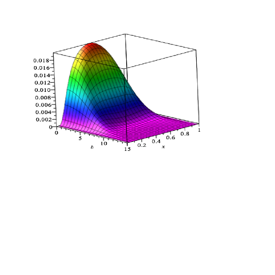
Figure 2: The normalized pion holographic wavefunction squared and summed over helicities, $|\Psi^{\pi}(x,\mathbf{b})|^{2}~{}[\text{GeV}^{2}]$, as a function of the transverse separation $b~{}[\text{GeV}^{-1}]$ and momentum fraction $x$. Upper: original. Lower left: spin-improved ($A=0,B=1$). Lower right: spin-improved ($A=1,B=1$). All plots are generated with $\kappa=523$ MeV and $m_{f}=330$ MeV.

III Radius and decay constant

Having specified our spin-improved holographic wavefunction, we shall now compute two observables: the pion radius, sensitive to long-distance (non-perturbative) physics and the pion decay constant, sensitive to short-distance (perturbative) physics. We shall predict both observables using the original and spin-improved holographic wavefunctions with a constituent quark mass, $m_{u/d}=330$ MeV. We expect to fit better the radius since the holographic pion wavefunction lacks the perturbative, short-distance corrections that may be required to accurately predict the decay constant.

The root-mean-square pion radius is given by Brodsky and de Teramond (2008a):

$$\sqrt{\langle r_{\pi}^{2}\rangle}=\left[\frac{3}{2}\int\mathrm{d}x\mathrm{d}^{2}\mathbf{b}[b(1-x)]^{2}|\Psi^{\pi}(x,\mathbf{b})|^{2}\right]^{1/2}$$ (25)

where $|\Psi^{\pi}(x,\mathbf{b})|^{2}$ is given by Eq. (24). Our predictions for the pion radius are compared to the measured value in Table 1. As can be seen, we achieve a much better agreement with the datum with the spin-improved holographic wavefunctions. It is worth noting the excellent agreement achieved with the ($A=1,B=1$) spin-improved wavefunction.

	$\sqrt{\langle r_{\pi}^{2}\rangle}$ [fm]
Original	$0.544$
Spin-improved ($A=0,B=1$)	$0.683$
Spin-improved ($A=1,B=1$)	$0.673$
Experiment Olive et al. (2014)	$0.672\pm 0.008$

Table 1: Our predictions for the pion radius using the holographic wavefunction with $\kappa=523$ MeV and $m_{u/d}=330$ MeV. The datum is from PDG 2014 Olive et al. (2014).

Note that if we compute the pion radius using the original holographic wavefunction but with $\kappa=540$ MeV and $m_{f}=330$ MeV as in Ref. Swarnkar and Chakrabarti (2015), we obtain $\sqrt{\langle r_{\pi}^{2}\rangle}=0.530$ fm which is to be compared with the prediction of Ref. Swarnkar and Chakrabarti (2015): $\sqrt{\langle r_{\pi}^{2}\rangle}=0.529$ fm. In Ref. Swarnkar and Chakrabarti (2015), the authors obtain the pion radius from the slope of the EM pion form factor $F_{\pi}(Q^{2})$ at $Q^{2}=0$ with the constraint that $F(0)=1$. We note that the latter constraint on the form factor is automatically satisfied if the pion wavefunction is normalized with $P_{q\bar{q}}=1$. Thus, although the authors of Ref. Swarnkar and Chakrabarti (2015) imply $P_{q\bar{q}}=0.62$ in order to fit the decay constant, they implicitly assume $P_{q\bar{q}}=1$ when computing the EM form factor. This is why we are able to reproduce their prediction for the pion radius even though we assume $P_{q\bar{q}}=1$.

We now compute the pion decay constant, $f_{\pi}$, defined by Lepage and Brodsky (1980)

$$\langle 0|\bar{\Psi}_{d}\gamma^{\mu}\gamma_{5}\Psi_{u}|\pi^{+}\rangle=f_{\pi}P^{\mu}$$ (26)

where we have omitted to write a conventional $\sqrt{2}i$ factor on the right-hand-side. Taking $\mu=+$ and expanding the left-hand-side of Eq. (26), we obtain

$$\langle 0|\bar{\Psi}_{d}\gamma^{+}\gamma^{5}\Psi_{u}|\pi^{+}\rangle=\sqrt{4\pi N_{c}}\sum_{h,\bar{h}}\int\frac{\mathrm{d}^{2}\mathbf{k}}{16\pi^{3}}\mathrm{d}x\Psi_{h,\bar{h}}^{\pi}(x,\mathbf{k})\left\{\frac{\bar{v}_{\bar{h}}}{\sqrt{1-x}}(\gamma^{+}\gamma^{5})\frac{u_{h}}{\sqrt{x}}\right\}\;.$$ (27)

The light-front matrix element in curly brackets can readily be evaluated:

$$\left\{\frac{\bar{v}_{\bar{h}}}{\sqrt{1-x}}(\gamma^{+}\gamma^{5})\frac{u_{h}}{\sqrt{x}}\right\}=2P^{+}(2h)\delta_{-h\bar{h}}\;,$$ (28)

which implies that only the opposite-helicities term in the holographic wavefunction contributes to the decay constant. We note, however, that the same-helicities term affects the normalization of our wavefunction and thus our prediction for the decay constant. Using our spin-improved wavefunction, Eq. (21), we deduce that

$$f_{\pi}=2\sqrt{\frac{N_{c}}{\pi}}\left.\int\mathrm{d}x\{A((x(1-x)M_{\pi}^{2})+Bm_{f}M_{\pi}\}\frac{\Psi^{\pi}(x,\zeta)}{x(1-x)}\right|_{\zeta=0}\;.$$ (29)

On the other hand, using the original holographic wavefunction, Eq. (22), we obtain

$$f^{\text{[o]}}_{\pi}=2\sqrt{6}\sqrt{4\pi}\int\mathrm{d}x\frac{\mathrm{d}^{2}\mathbf{k}}{16\pi^{3}}\Psi(x,\mathbf{k})=2\sqrt{2}\sqrt{\frac{N_{c}}{4\pi}}\left.\int\mathrm{d}x\Psi^{\pi}(x,\zeta)\right|_{\zeta=0}$$ (30)

where we have written the momentum-space expression to point out that, up to a factor of $\sqrt{4\pi}$, it coincides with the formula for the decay constant given in Ref. Lepage et al. (1982) and widely used in the literature, as for example, in Refs. Chabysheva and Hiller (2013); Swarnkar and Chakrabarti (2015); Branz et al. (2010). The $\sqrt{4\pi}$ factor mismatch is consistent with the fact that our normalization in momentum-space (Eq. (12)) differs from the conventional light-front normalization Lepage and Brodsky (1980) by a factor of $4\pi$.

Our predictions for the pion decay constant are shown in Table 2. As can be seen, we achieve a much better agreement with the datum with the spin-improved holographic wavefunctions although we still somewhat overestimate the measured value. As we noted above, this could perhaps be attributed to the fact that perturbative corrections are not included in the holographic pion wavefunction.

	$f_{\pi}$ [MeV]
Original	$161$
Spin-improved ($A=0,B=1$)	$135$
Spin-improved ($A=1,B=1$)	$138$
Experiment Olive et al. (2014)	$130.4\pm 0.04\pm 0.2$

Table 2: Our predictions for the pion decay constant using the holographic wavefunction with $\kappa=523$ MeV and $m_{u/d}=330$ MeV. The datum is from PDG 2014 Olive et al. (2014).

IV EM form factor

We now compute the pion EM form factor defined as

$$\langle\pi^{+}:P^{\prime}|J_{\text{em}}^{\mu}(0)|\pi^{+}:P\rangle=2(P+P^{\prime})^{\mu}F_{\pi}(Q^{2})$$ (31)

where $P^{\prime}=P+q$, $Q^{2}=-q^{2}$ and the EM current $J_{\text{em}}^{\mu}(z)=\sum_{f}e_{f}\bar{\Psi}(z)\gamma^{\mu}\Psi(z)$ with $f=\bar{d},u$ and $e_{\bar{d},u}=1/3,2/3$. The EM form factor can be expressed in terms of the pion LFWF using the Drell-Yan-West formula Drell and Yan (1970); West (1970):

$$F_{\pi}(Q^{2})=2\pi\int\mathrm{d}x\mathrm{d}b~{}b~{}J_{0}[(1-x)bQ]~{}|\Psi^{\pi}(x,\textbf{b})|^{2}$$ (32)

where $|\Psi^{\pi}(x,\textbf{b})|^{2}$ is given by Eq. (24). Note that Eq. (32) implies that $F_{\pi}(0)=1$ if the pion LFWF is normalized according to Eq. (23) and that the slope of the EM form factor at $Q^{2}=0$ is related to the mean radius of the pion given by Eq. (25) via

$$\langle r_{\pi}^{2}\rangle=-\frac{6}{F_{\pi}(0)}\left.\frac{\mathrm{d}F_{\pi}}{\mathrm{d}Q^{2}}\right|_{Q^{2}=0}\;.$$ (33)

Our predictions for the EM form factor using the original (dotted-orange curve) and our higher twist spin-improved (continuous-red and dashed-blue curve) are compared with the data from CERN et al (NA7 collaboration), CEA et al (1973), Cornell et al (1974, 1976, 1978), Jlab et al (The Jefferson Lab F$\pi$ Collaboration, The Jefferson Lab F$\pi$ Collaboration) and CLEO et al (CLEO collaboration); Seth et al. (2013) in Figure 3. As can be seen, the agreement with data is very much improved with the spin-improved holographic wavefunctions. In fact, we achieve excellent agreement with data from the lowest $Q^{2}$ datum to $Q^{2}\approx 7~{}\text{GeV}^{2}$. For $Q^{2}>7~{}\text{GeV}^{2}$, our predictions with the original and the spin-improved holographic wavefunctions coincide and they both undershoot the precise CLEO data et al (CLEO collaboration). This is the short-distance regime where perturbative corrections, not taken into account in the purely non-perturbative holographic wavefunction, become important. It is worth highlighting that agreement with the precise data in the non-perturbative region, $Q^{2}\leq 1~{}\text{GeV}^{2}$, is excellent with our higher twist spin-improved holographic wavefunctions.

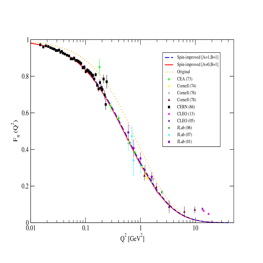
Figure 3: Our predictions for the pion EM form factor. Dotted-orange: original. Continuous-red curve: spin-improved ($A=0,B=1$). Dashed-blue curve: spin-improved ($A=1,B=1$). All theory curves generated with $\kappa=523$ MeV and $m_{f}=330$ MeV. Data from et al (NA7 collaboration); et al (1974, 1976, 1978); et al (The Jefferson Lab F$\pi$ Collaboration, The Jefferson Lab F$\pi$ Collaboration); et al (CLEO collaboration); Seth et al. (2013).

V Distribution Amplitude and transition form factor

We can also predict the twist-$2$ holographic pion DA, $\varphi_{\pi}(x,\mu)$, defined as Radyushkin (1977); Lepage and Brodsky (1980)

$$\langle 0|\bar{\Psi}_{d}(z)\gamma^{+}\gamma_{5}\Psi_{u}(0)|\pi^{+}\rangle=f_{\pi}P^{+}\int\mathrm{d}xe^{ix(P\cdot z)}\varphi_{\pi}(x,\mu)$$ (34)

where $z^{2}=0$. The DA is conventionally normalized as

$$\int\mathrm{d}x\varphi_{\pi}(x,\mu)=1$$ (35)

such that taking the limit of local operators ($z\to 0$) in Eq. (34), we recover the definition of the pion decay constant given by Eq. (26) (with $\mu=+$). Proceeding in the same manner as for the decay constant, we are able to show that

$$f_{\pi}\varphi_{\pi}(x,\mu)=2\sqrt{\frac{N_{c}}{\pi}}\int\mathrm{d}bJ_{0}(\mu b)b\{A((x(1-x)M_{\pi}^{2})+Bm_{f}M_{\pi}\}\frac{\Psi^{\pi}(x,\zeta)}{x(1-x)}\;.$$ (36)

In Figure 4, we compare our spin-improved holographic DAs to the original holographic DA and to the asymptotic DA as predicted in pQCD: $\varphi_{\pi}(x,\infty)=6x(1-x)$. It can be seen that our spin-improved holographic DAs (continuous-red and dashed-blue curves) are broader than both the original holographic DA (dotted-orange curve) and the asymptotic DA (dotted-black curve). All holographic DAs are both generated with $\mu=1$ GeV and we note they hardly evolve for $\mu>1$ GeV. In other words, our holographic DAs lack the hard, perturbative evolution given by the Efremov-Radyushkin-Brodsky-Lepage (ERBL) equations Lepage and Brodsky (1979); Efremov and Radyushkin (1980a, b). In Figure 5, we show the soft evolution of our spin-improved $(A=0,B=1)$ holographic DA between $\mu=0.3$ GeV and $\mu=1$ GeV. Implementing the ERLB evolution, as is done in Ref. Brodsky et al. (2011b), will allow our spin-improved holographic DA to evolve beyond $\mu=1$ GeV onto the asymptotic DA.

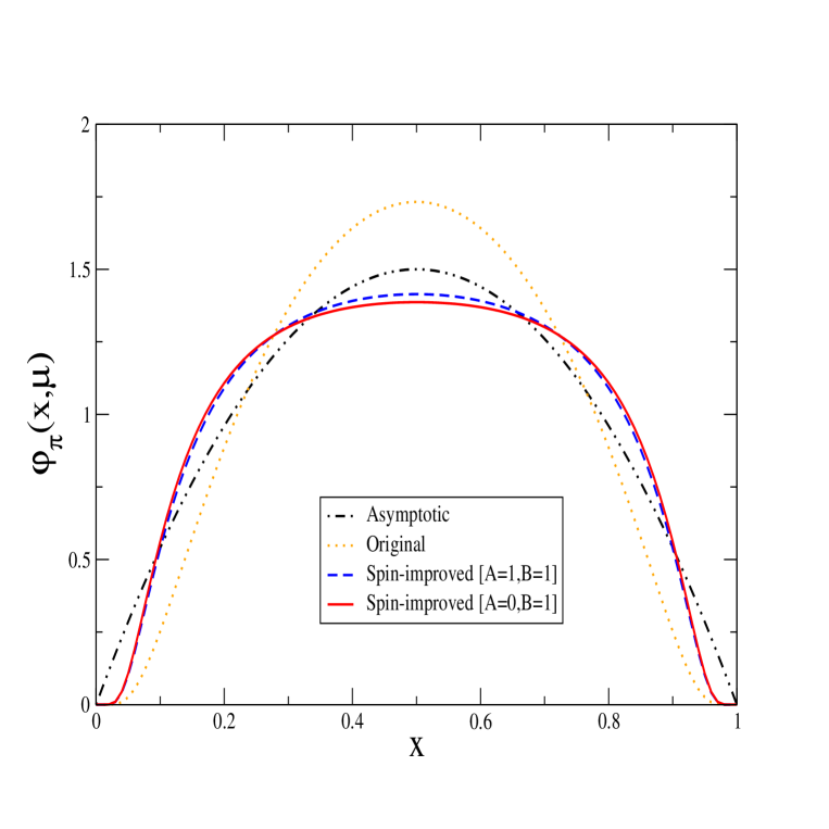
Figure 4: Comparing our spin-improved holographic DAs (continuous-red and dashed-blue curves) to the original holographic DA (dotted-orange curve) at a scale $\mu=1$ GeV, both with $\kappa=523$ MeV and $m_{f}=330$ MeV. The asymptotic DA is the dotted black curve.

Figure 5: The soft evolution of our ($(A=1,B=1)$) spin-improved holographic pion DA at a scale $\mu=0.3$ GeV(dot-dot-dashed-orange), $\mu=0.5$ GeV (dashed-blue), $\mu=0.7$ GeV (dot-dashed-magenta) and $\mu\geq 1$ GeV (continuous-red). The asymptotic DA is the dotted-black curve.

In order to compare our holographic DAs with the predictions of standard non-perturbative methods such as lattice QCD and QCD Sum Rules, we compute the moments defined as

$$\langle\xi_{n}\rangle=\int_{0}^{1}\mathrm{d}x(2x-1)^{n}\varphi_{\pi}(x,\mu)$$ (37)

and its inverse moment is given by

$$\langle x^{-1}\rangle=\int_{0}^{1}\mathrm{d}x\frac{\varphi_{\pi}(x,\mu)}{x}\;.$$ (38)

Our predictions for the first two non-vanishing moments $\langle\xi_{2}\rangle$ and $\langle\xi_{4}\rangle$ as well as the inverse moment are shown in Table 3. As can be seen, with the spin-improved holographic DAs, we achieve better agreement with the predictions of lattice QCD and QCD Sum Rules. However, our predicted moments turn out to be smaller than the predictions of all non-perturbative methods cited here. Our predicted moments are also smaller than the corresponding moments of the asymptotic DA. This discrepancy could be an indication that all dynamical spin effects might not fully captured by fixing $B=1$.

DA	$\mu$ [GeV]	$\langle\xi_{2}\rangle$	$\langle\xi_{4}\rangle$	$\langle x^{-1}\rangle$
Asymptotic	$\infty$	$0.2$	$0.085$	$3$
LFH spin-improved ($A=1,B=1$)	$\sim 1$	$0.195$	$0.076$	$2.74$
LFH spin-improved ($A=0,B=1$)	$\sim 1$	$0.199$	$0.078$	$2.76$
LFH (original)	$\sim 1$	$0.151$	$0.050$	$2.50$
LF Quark Model Choi and Ji (2007)	$\sim 1$	$0.24[0.22]$	$0.11[0.09]$
Sum Rules Ball and Zwicky (2005)	$1$	$0.24$	$0.11$
Renormalon model Agaev (2005)	$1$	$0.28$	$0.13$
Instanton vacuum Petrov et al. (1999); Nam et al. (2006)	$1$	$0.22,0.21$	$0.10,0.09$
Lattice Braun et al. (2015, 2006)	$2$	$0.2361(41)(39),0.27\pm 0.04$
NLC Sum Rules Bakulev et al. (2001)	$2$	$0.248^{+0.016}_{-0.015}$	$0.108^{+0.05}_{-0.03}$	$3.16^{+0.09}_{-0.09}$
Sum RulesChernyak and Zhitnitsky (1984)	$2$	$0.343$	$0.181$	$4.25$
Dyson-Schwinger[RL,DB]Chang et al. (2013)	$2$	$0.280,0.251$	$0.151,0.128$	$5.5,4.6$
Platykurtic Stefanis (2014)	$2$	$0.220^{+0.009}_{-0.006}$	$0.098^{+0.008}_{-0.005}$	$3.13^{+0.14}_{-0.10}$

Table 3: Our predictions for the first two non-vanishing moments and the inverse moment of the pion holographic twist-$2$ DA with $\kappa=523$ MeV and $m_{f}=330$ MeV, compared to the predictions of lattice QCD by Braun et al. in 2006 Braun et al. (2006) and 2015 Braun et al. (2015), QCD Sum Rules with non-local condensates by Bakulaev et al. Bakulev et al. (2001), QCD Sum Rules by Chernyak and Zhitnitsky Chernyak and Zhitnitsky (1984), QCD Sum Rules by Ball and Zwicky Ball and Zwicky (2005), light-front quark model of Choi and Ji with two different potentials Choi and Ji (2007), renormalon model of Agaev Agaev (2005), instanton vacuum models of Petrov et al. Petrov et al. (1999) and Nam et al. Nam et al. (2006), Dyson-Schwinger Equations of Chang et al. Chang et al. (2013) in the rainbow-ladder (RL) approximation and using the dynamical chiral symmetry breaking improved kernel (DB) and finally the platykurtic DA of Stefanis et al. Stefanis (2014); Stefanis et al. (2015).

Using our holographic DAs, we are able to predict the photon-to-pion transition form factor (TFF) which, to leading order in pQCD, is given as Lepage and Brodsky (1980)

$$F_{\gamma\pi}(Q^{2})=\frac{\sqrt{2}}{3}f_{\pi}\int_{0}^{1}\mathrm{d}x\frac{\varphi_{\pi}(x,xQ)}{Q^{2}x}\;.$$ (39)

We note that, even when computing the TFF in the perturbative region $Q^{2}\geq 1~{}\text{GeV}^{2}$, the DA itself is probed at a scale $\mu=xQ$, which can be low if $x$ is close to its end-points. Figure 6 shows that our spin-improved holographic DAs (continuous-red and dashed-blue curves) do a better job than the original holographic DA (dotted-orange curve). We note that the BaBar (2009) data et al (BaBar collaboration) indicate a strong scaling violation in disagreement with the Brodsky-Lepage limit: $F_{\pi\gamma^{*}\gamma}(Q^{2}\to\infty)=\sqrt{2}f_{\pi}$ obtained by substituting the asymptotic DA in Eq. (39) and shown as the dotted-black curves in Figure 6. The more recent Belle (2012) data et al (Belle collaboration) do not confirm the BaBar (2009) data for $Q^{2}>10~{}\text{GeV}^{2}$ and the issue is likely to be resolved by precise future measurements in this kinematic range. Our spin-improved holographic wavefunctions clearly cannot describe the strong scaling violation indicated by the BaBar(2009) data and neither do our predictions exceed the asymptotic Brodsky-Lepage limit. For alternative models of the pion DA which are able to accommodate the BaBar (2009) data, we refer to Refs. Radyushkin (2009); Polyakov (2009); Li and Mishima (2009) and for an exhaustive analysis of the TFF data, we refer to Bakulev et al. (2012).

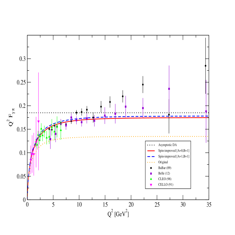
Figure 6: Our predictions for the photon-to-pion TFF as a function of the photon’s virtuality, $Q^{2}$. Dotted-orange curve: original DA. Continuous-red and dashed-blue curves: spin-improved with $[A=0,B=1]$ and $[A=1,B=1]$ respectively. All theory curves are generated with $\kappa=523$ MeV and $m_{f}=330$ MeV. The dotted black curve is generated using the asymptotic DA with the measured pion decay constant. For asymptotic $Q^{2}$, they indicate the Brodsky-Lepage limit. The data are from CELLO et al (CELLO collaboration), CLEO et al (CLEO collaboration), BaBar et al (Belle collaboration) and Belle et al (Belle collaboration).

VI Conclusions

We have accounted for dynamical spin effects in the holographic pion light-front wavefunction and found a remarkable improvement in the description of pion radius, decay constant, EM form factor and photon-to-pion TFF. To generate our predictions, we have used a constituent quark mass of $330$ MeV and the universal AdS/QCD scale $\kappa=523$ MeV, together with the assumption that the pion consists only of the leading quark-antiquark Fock state. Our results suggest that it could be possible to have a unified treatment of all light mesons, including the pion, with a universal fundamental AdS/QCD scale which fits the baryon and meson Regge slopes and also accurately predicts the non-perturbative QCD scale $\Lambda_{\text{QCD}}^{\overline{MS}}$. We also found that the predicted moments for the spin-improved holographic pion twist-$2$ DA are in better agreement with the predictions of standard non-perturbative methods such as lattice QCD and QCD Sum Rules, although they remain smaller than the latter. This suggests that tuning the values of $A$ and $B$ could be necessary or, at a deeper level, that the assumption underlying our Eq. (13) might not capturing all the dynamical spin effects in the pion. But this assumption, together with $(A=0,1;B=1)$, does bring a significant improvement in the description of all available experimental data without necessarily having to use a much smaller AdS/QCD scale and/or invoke higher Fock states contributions exclusively for the pion. Our findings thus support the idea of the emergence of a universal AdS/QCD confinement scale $\kappa$.

VII Acknowledgements

The work of M.A and R.S is supported by a team grant from National Science and Engineering Research Council of Canada (NSERC). F.C and R.S thank Mount Allison University for hospitality where parts of this work were carried out. We thank J. R. Forshaw, N. Stefanis and G. de Téramond for useful comments on the first version of this paper.

References

- Horn and Roberts (2016) T. Horn and C. D. Roberts, J. Phys. G43, 073001 (2016), eprint 1602.04016.
- Ali (2016) A. Ali, Int. J. Mod. Phys. A31, 1630036 (2016), eprint 1607.04918.
- Brodsky et al. (2015) S. J. Brodsky, G. F. de Teramond, H. G. Dosch, and J. Erlich, Phys. Rept. 584, 1 (2015), eprint 1407.8131.
- Brodsky et al. (1998) S. J. Brodsky, H.-C. Pauli, and S. S. Pinsky, Phys. Rept. 301, 299 (1998), eprint hep-ph/9705477.
- de Teramond and Brodsky (2009) G. F. de Teramond and S. J. Brodsky, Phys. Rev. Lett. 102, 081601 (2009), eprint 0809.4899.
- Brodsky and de Teramond (2006) S. J. Brodsky and G. F. de Teramond, Phys. Rev. Lett. 96, 201601 (2006), eprint hep-ph/0602252.
- de Teramond and Brodsky (2005) G. F. de Teramond and S. J. Brodsky, Phys. Rev. Lett. 94, 201601 (2005), eprint hep-th/0501022.
- Brodsky and de Teramond (2008a) S. J. Brodsky and G. F. de Teramond, Phys. Rev. D77, 056007 (2008a), eprint 0707.3859.
- Brodsky et al. (2016) S. J. Brodsky, G. F. de Téramond, H. G. Dosch, and C. Lorcé, Int. J. Mod. Phys. A31, 1630029 (2016), eprint 1606.04638.
- Brodsky et al. (2014) S. J. Brodsky, G. F. De Téramond, and H. G. Dosch, Phys. Lett. B729, 3 (2014), eprint 1302.4105.
- Brodsky et al. (2013) S. J. Brodsky, G. F. de Téramond, and H. G. Dosch, Nuovo Cim. C036, 265 (2013), eprint 1302.5399.
- de Alfaro et al. (1976) V. de Alfaro, S. Fubini, and G. Furlan, Nuovo Cim. A34, 569 (1976).
- Brodsky and de Teramond (2008b) S. J. Brodsky and G. F. de Teramond, Phys. Rev. D78, 025032 (2008b), eprint 0804.0452.
- Glazek and Trawiński (2013) S. D. Glazek and A. P. Trawiński, Phys. Rev. D88, 105025 (2013), eprint 1307.2059.
- Swarnkar and Chakrabarti (2015) R. Swarnkar and D. Chakrabarti, Phys. Rev. D92, 074023 (2015), eprint 1507.01568.
- Brodsky and de Teramond (2009) S. J. Brodsky and G. F. de Teramond, Subnucl. Ser. 45, 139 (2009), eprint 0802.0514.
- Brodsky et al. (2010) S. J. Brodsky, G. F. de Teramond, and A. Deur, Phys. Rev. D81, 096010 (2010), eprint 1002.3948.
- Deur et al. (2016) A. Deur, S. J. Brodsky, and G. F. de Teramond (2016), eprint 1608.04933.
- Forshaw and Sandapen (2012) J. R. Forshaw and R. Sandapen, Phys. Rev. Lett. 109, 081601 (2012), eprint 1203.6088.
- Ahmady et al. (2016) M. Ahmady, R. Sandapen, and N. Sharma (2016), eprint 1605.07665.
- Sufian et al. (2016) R. S. Sufian, G. F. de Téramond, S. J. Brodsky, A. Deur, and H. G. Dosch (2016), eprint 1609.06688.
- Brodsky et al. (2011a) S. J. Brodsky, F.-G. Cao, and G. F. de Teramond, Phys. Rev. D84, 075012 (2011a), eprint 1105.3999.
- Drell and Yan (1970) S. D. Drell and T.-M. Yan, Phys. Rev. Lett. 24, 181 (1970).
- West (1970) G. B. West, Phys. Rev. Lett. 24, 1206 (1970).
- Vega and Schmidt (2009) A. Vega and I. Schmidt, Phys. Rev. D79, 055003 (2009), eprint 0811.4638.
- Vega et al. (2009) A. Vega, I. Schmidt, T. Branz, T. Gutsche, and V. E. Lyubovitskij, Phys. Rev. D80, 055014 (2009), eprint 0906.1220.
- Branz et al. (2010) T. Branz, T. Gutsche, V. E. Lyubovitskij, I. Schmidt, and A. Vega, Phys. Rev. D82, 074022 (2010), eprint 1008.0268.
- Lepage and Brodsky (1980) G. P. Lepage and S. J. Brodsky, Phys. Rev. D22, 2157 (1980).
- Dosch et al. (1997) H. G. Dosch, T. Gousset, G. Kulzinger, and H. J. Pirner, Phys. Rev. D55, 2602 (1997), eprint hep-ph/9608203.
- Kulzinger et al. (1999) G. Kulzinger, H. G. Dosch, and H. J. Pirner, Eur. Phys. J. C7, 73 (1999), eprint hep-ph/9806352.
- Nemchik et al. (1997) J. Nemchik, N. N. Nikolaev, E. Predazzi, and B. G. Zakharov, Z. Phys. C75, 71 (1997), eprint hep-ph/9605231.
- Forshaw et al. (2004) J. R. Forshaw, R. Sandapen, and G. Shaw, Phys. Rev. D69, 094013 (2004), eprint hep-ph/0312172.
- Watt and Kowalski (2008) G. Watt and H. Kowalski, Phys. Rev. D78, 014016 (2008), eprint 0712.2670.
- Forshaw et al. (2006) J. R. Forshaw, R. Sandapen, and G. Shaw, JHEP 11, 025 (2006), eprint hep-ph/0608161.
- Forshaw and Sandapen (2010) J. R. Forshaw and R. Sandapen, JHEP 11, 037 (2010), eprint 1007.1990.
- Forshaw and Sandapen (2011) J. R. Forshaw and R. Sandapen, JHEP 10, 093 (2011), eprint 1104.4753.
- Armesto and Rezaeian (2014) N. Armesto and A. H. Rezaeian, Phys. Rev. D90, 054003 (2014), eprint 1402.4831.
- Rezaeian and Schmidt (2013) A. H. Rezaeian and I. Schmidt, Phys. Rev. D88, 074016 (2013), eprint 1307.0825.
- Goncalves et al. (2016) V. P. Goncalves, F. S. Navarra, and D. Spiering, J. Phys. G43, 095002 (2016), eprint 1510.01512.
- Rezaeian et al. (2013) A. H. Rezaeian, M. Siddikov, M. Van de Klundert, and R. Venugopalan, Phys. Rev. D87, 034002 (2013), eprint 1212.2974.
- Heinzl (2001) T. Heinzl, Lect. Notes Phys. 572, 55 (2001), eprint hep-th/0008096.
- Heinzl (2000) T. Heinzl, Nucl. Phys. Proc. Suppl. 90, 83 (2000), [,231(2000)], eprint hep-ph/0008314.
- Dziembowski (1988) Z. Dziembowski, Phys. Rev. D37, 778 (1988).
- Jaus (1990) W. Jaus, Phys. Rev. D41, 3394 (1990).
- Ji and Cotanch (1990) C. R. Ji and S. R. Cotanch, Phys. Rev. D41, 2319 (1990).
- Ji et al. (1992) C. R. Ji, P. L. Chung, and S. R. Cotanch, Phys. Rev. D45, 4214 (1992).
- Choi and Ji (2007) H.-M. Choi and C.-R. Ji, Phys. Rev. D75, 034019 (2007), eprint hep-ph/0701177.
- Trawiński (2016) A. P. Trawiński, Few Body Syst. 57, 449 (2016).
- Chang et al. (2016) Q. Chang, S. J. Brodsky, and X.-Q. Li (2016), eprint 1612.05298.
- Leutwyler (1974a) H. Leutwyler, Nucl. Phys. B76, 413 (1974a).
- Leutwyler (1974b) H. Leutwyler, Phys. Lett. B48, 45 (1974b).
- Brodsky et al. (2006) S. J. Brodsky, S. Gardner, and D. S. Hwang, Phys. Rev. D73, 036007 (2006), eprint hep-ph/0601037.
- Olive et al. (2014) K. A. Olive et al. (Particle Data Group), Chin. Phys. C38, 090001 (2014).
- Lepage et al. (1982) G. P. Lepage, S. J. Brodsky, T. Huang, and P. B. Mackenzie, in Particles and Fields 2. Proceedings, Summer Institute, BANFF, Canada, August 16-27, 1981 (1982), pp. 83–141, URL http://lss.fnal.gov/archive/preprint/fermilab-conf-81-114-t.shtml.
- Chabysheva and Hiller (2013) S. S. Chabysheva and J. R. Hiller, Annals Phys. 337, 143 (2013), eprint 1207.7128.
- et al (NA7 collaboration) S. R. A. et al (NA7 collaboration), Nucl. Phys. B277, 168 (1986).
- et al (1973) C. N. B. et al, Phys. Rev. D8, 92 (1973).
- et al (1974) C. J. B. et al, Phys. Rev. D9, 1229 (1974).
- et al (1976) C. J. B. et al, Phys. Rev. D13, 25 (1976).
- et al (1978) C. J. B. et al, Phys. Rev. D17, 1693 (1978).
- et al (The Jefferson Lab F Collaboration) J. V. et al (The Jefferson Lab F Collaboration), Phys. Rev. Lett. 86, 1713 (2001), eprint hep-ph/0602252.
- et al (The Jefferson Lab F Collaboration) T. H. et al (The Jefferson Lab F Collaboration), Phys. Rev. Lett. 97, 192001 (2006), eprint nucl-ex/0607005.
- et al (CLEO collaboration) T. K. P. et al (CLEO collaboration), Phys. Rev. Lett. 95, 261803 (2005), eprint hep-ex/0510005.
- Seth et al. (2013) K. K. Seth, S. Dobbs, Z. Metreveli, A. Tomaradze, T. Xiao, and G. Bonvicini, Phys. Rev. Lett. 110, 022002 (2013), eprint 1210.1596.
- Radyushkin (1977) A. V. Radyushkin, Submitted to: Phys. Lett. (1977), eprint hep-ph/0410276.
- Lepage and Brodsky (1979) G. P. Lepage and S. J. Brodsky, Phys. Lett. B87, 359 (1979).
- Efremov and Radyushkin (1980a) A. V. Efremov and A. V. Radyushkin, Theor. Math. Phys. 42, 97 (1980a), [Teor. Mat. Fiz.42,147(1980)].
- Efremov and Radyushkin (1980b) A. V. Efremov and A. V. Radyushkin, Phys. Lett. B94, 245 (1980b).
- Brodsky et al. (2011b) S. J. Brodsky, F.-G. Cao, and G. F. de Teramond, Phys. Rev. D84, 033001 (2011b), eprint 1104.3364.
- Ball and Zwicky (2005) P. Ball and R. Zwicky, Phys. Rev. D71, 014015 (2005), eprint hep-ph/0406232.
- Agaev (2005) S. S. Agaev, Phys. Rev. D72, 114010 (2005), [Erratum: Phys. Rev.D73,059902(2006)], eprint hep-ph/0511192.
- Petrov et al. (1999) V. Yu. Petrov, M. V. Polyakov, R. Ruskov, C. Weiss, and K. Goeke, Phys. Rev. D59, 114018 (1999), eprint hep-ph/9807229.
- Nam et al. (2006) S.-i. Nam, H.-C. Kim, A. Hosaka, and M. M. Musakhanov, Phys. Rev. D74, 014019 (2006), eprint hep-ph/0605259.
- Braun et al. (2015) V. M. Braun, S. Collins, M. Göckeler, P. Pérez-Rubio, A. Schäfer, R. W. Schiel, and A. Sternbeck, Phys. Rev. D92, 014504 (2015), eprint 1503.03656.
- Braun et al. (2006) V. M. Braun et al., Phys. Rev. D74, 074501 (2006), eprint hep-lat/0606012.
- Bakulev et al. (2001) A. P. Bakulev, S. V. Mikhailov, and N. G. Stefanis, Phys. Lett. B508, 279 (2001), [Erratum: Phys. Lett.B590,309(2004)], eprint hep-ph/0103119.
- Chernyak and Zhitnitsky (1984) V. L. Chernyak and A. R. Zhitnitsky, Phys. Rept. 112, 173 (1984).
- Chang et al. (2013) L. Chang, I. C. Cloet, J. J. Cobos-Martinez, C. D. Roberts, S. M. Schmidt, and P. C. Tandy, Phys. Rev. Lett. 110, 132001 (2013), eprint 1301.0324.
- Stefanis (2014) N. G. Stefanis, Phys. Lett. B738, 483 (2014), eprint 1405.0959.
- Stefanis et al. (2015) N. G. Stefanis, S. V. Mikhailov, and A. V. Pimikov, Few Body Syst. 56, 295 (2015), eprint 1411.0528.
- et al (BaBar collaboration) B. A. et al (BaBar collaboration), Phys. Rev. D80, 052002 (2009), eprint 0905.4778.
- et al (Belle collaboration) S. U. et al (Belle collaboration), Phys. Rev. D86, 092007 (2012), eprint 1205.3249.
- Radyushkin (2009) A. V. Radyushkin, Phys. Rev. D80, 094009 (2009), eprint 0906.0323.
- Polyakov (2009) M. V. Polyakov, JETP Lett. 90, 228 (2009), eprint 0906.0538.
- Li and Mishima (2009) H.-n. Li and S. Mishima, Phys. Rev. D80, 074024 (2009), eprint 0907.0166.
- Bakulev et al. (2012) A. P. Bakulev, S. V. Mikhailov, A. V. Pimikov, and N. G. Stefanis, Phys. Rev. D86, 031501 (2012), eprint 1205.3770.
- et al (CELLO collaboration) H. J. B. et al (CELLO collaboration), Z. Phys. C49, 401 (1991).
- et al (CLEO collaboration) J. G. et al (CLEO collaboration), Phys. Rev. D57, 33 (1998), eprint hep-ex/9707031.