Efficient unitary designs with nearly time-independent Hamiltonian dynamics

Abstract

We provide new constructions of unitary $t$-designs for general $t$ on one qudit and $N$ qubits, and propose a design Hamiltonian, a random Hamiltonian of which dynamics always forms a unitary design after a threshold time, as a basic framework to investigate randomising time evolution in quantum many-body systems. The new constructions are based on recently proposed schemes of repeating random unitaires diagonal in mutually unbiased bases. We first show that, if a pair of the bases satisfies a certain condition, the process on one qudit approximately forms a unitary $t$-design after $O(t)$ repetitions. We then construct quantum circuits on $N$ qubits that achieve unitary $t$-designs for $t=o(N^{1/2})$ using $O(tN^{2})$ gates, improving the previous result using $O(t^{10}N^{2})$ gates in terms of $t$. Based on these results, we present a design Hamiltonian with periodically changing two-local spin-glass-type interactions, leading to fast and relatively natural realisations of unitary designs in complex many-body systems.

I Introduction

Random quantum processes play important roles in quantum information processing, as one of the fundamental primitives in quantum Shannon theory D2005 ; DW2004 ; GPW2005 ; ADHW2009 ; HaydenTutorial ; DBWR2010 ; SDTR2013 ; HM14 and as a useful resource to demonstrate quantum advantages in many protocols EAZ2005 ; KLRetc2008 ; MGE2011 ; MGE2012 ; S2005 ; BH2013 ; KRT2014 ; KL15 ; KZD2016 ; OAGKAL2016 . In recent years, random processes have been also revealed to be the key to understanding fundamental physics in complex quantum systems, leading to new developments in quantum thermodynamics PSW2006 ; GLTZ2006 ; R2008 (see Ref. GE2016 for a comprehensive review), black hole information science HP2007 ; SS2008 ; S2011 ; LSHOH2013 ; S2014 ; HQRY2016 and strongly correlated many-body physics SS2014 ; RD2015 ; SS2015 . In quantum systems, random processes are often represented by random unitaries drawn uniformly at random according to the Haar measure, referred to as Haar random unitaries. However, when a system consists of a large number of particles, it is highly inefficient to implement Haar random unitaries, implying that they rarely appear in natural systems composed of many particles especially when the interactions are local. This fact has lead to the research area on finite-degree approximations of Haar random unitaries, so-called unitary designs DLT2002 ; DCEL2009 ; GAE2007 , and their efficient implementations TGJ2007 ; BWV2008a ; WBV2008 ; HL2009 ; DJ2011 ; HL2009TPE ; BHH2012 ; CLLW2015 ; NHMW2015-1 ; Z2015 ; W2015 . A unitary $t$-design is called exact when it simulates all the first $t$ moments of Haar random unitaries and approximate when the simulations are with errors.

Traditionally, unitary $t$-designs have been studied for small $t$. In particular, unitary $2$-designs were intensely studied DLT2002 ; BWV2008a ; WBV2008 ; GAE2007 ; TGJ2007 ; DCEL2009 ; HL2009 ; DJ2011 ; BWV2008a ; WBV2008 ; CLLW2015 ; NHMW2015-1 due to the facts that they are useful in important tasks, such as decoupling HaydenTutorial ; DBWR2010 ; SDTR2013 ; HM14 and randomised benchmarking EAZ2005 ; KLRetc2008 ; MGE2011 ; MGE2012 , and that the Clifford group is an exact unitary $2$-design DLT2002 . Later, the Clifford group on qubits was also shown to be a unitary $3$-design but not to be a $4$-design Z2015 ; W2015 ; ZKGD2016 . For $t\geq 4$, a few applications are known (e.g. state discrimination S2005 , quantum speed-ups in query complexity BH2013 and compressed sensing KRT2014 ; KZD2016 ), but they are of potential importance when strong large deviation bounds are needed. So far, only a couple of efficient implementations for $t\geq 4$ are known to the best of our knowledge. One is to use a classical tensor product expander and the Fourier transformation, forming approximate unitary $t$-designs for $t=O(N/\log N)$ by using ${\rm poly}(N)$ quantum gates HL2009TPE . The other is to use local random quantum circuits composed of random two-qubit gates applied onto neighbouring qubits, which achieves approximate unitary $t$-designs for $t={\rm poly}(N)$ using $O(t^{10}N^{2})$ gates BHH2012 .

Despite these implementations of unitary designs by quantum circuits, there exists a certain gap between the constructions and physically feasible dynamics in quantum many-body systems. The constructions require a finely structured circuit HL2009TPE or the use of randomly varying interactions BHH2012 , while dynamics in physically feasible many-body systems is typically not structured and is generated by a Hamiltonian, which may slightly fluctuate over time but should be based on time-independent one. Indeed, if we interpret local random quantum circuits on $N$ qubits in terms of Hamiltonian dynamics, the interactions should be changed uniformly at random $O(t^{10}N)$ times before the dynamics achieves unitary $t$-designs. Due to its dependence on the number of particles, the total Hamiltonian should be highly time-dependent and may not be so physically feasible in large systems, resulting in a lack of solid basis of a number of studies of fundamental phenomena in many-body systems based on random dynamics PSW2006 ; GLTZ2006 ; R2008 ; GE2016 ; HP2007 ; SS2008 ; S2011 ; LSHOH2013 ; S2014 ; HQRY2016 . There is also an increasing demand from black hole information science and quantum chaos to fully understand microscopic dynamics of randomisation, where so-called scrambling has been intensely studied HP2007 ; SS2008 ; S2011 ; LSHOH2013 ; S2014 ; HQRY2016 ; SS2014 ; RD2015 ; SS2015 . As scrambling is a weak variant of unitary designs, studying natural Hamiltonians generating unitary designs will bring better understandings in the context. Further, implementations of unitary designs by Hamiltonian dynamics are of practical importance, helping experimental realisations of designs, as any quantum circuit is fundamentally implemented by engineering Hamiltonians.

In this paper, we provide new constructions of unitary $t$-designs and propose a design Hamiltonian, a random Hamiltonian of which dynamics forms a unitary design at any time after a threshold time. The constructions are based on the scheme of repeating random unitaries diagonal in mutually unbiased bases NM2013 ; NM2014 ; NHMW2015-1 ; NHMW2015-2 . We first show that the process on one qudit achieves unitary $t$-designs after $O(t)$ repetitions if a pair of the two bases satisfies a certain condition, which is met by a pair of any basis and its Fourier basis and that of the Pauli-$X$ and -$Z$ bases. As the construction works for any space, it will be useful to implement unitary designs in a subspace, such as a symmetric subspace, which is known to demonstrate a quantum advantage in metrology OAGKAL2016 . We then focus on $N$-qubit systems and investigate efficient implementations of random unitaries diagonal in the Pauli-$Z$ basis by quantum circuits. By mapping this problem to a combinatorial problem called a local permutation check problem, which can be further reduced to a special type of constrained problems in extremal algebraic theory AAK2003 ; AAK2003-2 , we prove that an approximate unitary $t$-design for $t=o(N^{1/2})$ can be achieved using $O(tN^{2})$ gates. In terms of $t$, this drastically improves the previous result BHH2012 using $O(t^{10}N^{2})$ gates and is essentially optimal. As higher-designs are useful to improve the performance of applications of lower-designs due to their large deviation bounds L2009LDB , this construction will contribute to improve applications of designs D2005 ; DW2004 ; GPW2005 ; ADHW2009 ; HaydenTutorial ; DBWR2010 ; SDTR2013 ; HM14 ; EAZ2005 ; KLRetc2008 ; MGE2011 ; MGE2012 ; S2005 ; BH2013 ; KRT2014 ; KL15 ; KZD2016 ; OAGKAL2016 . Finally, we introduce design Hamiltonians and present a nearly time-independent one with spin-glass-type interactions, where the interactions need to be varied only $O(t)$ times before the corresponding time-evolution operators form unitary $t$-designs. As a simple consequence, the design Hamiltonians quickly saturate the so-called out-of-time-ordered correlators SS2014 ; RD2015 ; SS2015 to the Haar averaged values, suggesting a close relation between the design Hamiltonians and quantum chaos. We also propose a conjecture about the timescale for a natural design Hamiltonian to generate unitary designs, which can be seen as a generalisation of the fast scrambling conjecture SS2008 .

The paper is organised as follows. In Section II, we introduce necessary notation and explain definitions and properties of random unitaries. All the main results are summarised in Section III, of which proofs are provided in Section IV. We conclude and discuss possible future directions in Section V. Small lemmas and propositions presented in the paper are proven in Appendices.

II Preliminaries

We use the following standard asymptotic notation. Let $f(n)$ and $g(n)$ be functions on $\mathbb{R}^{+}$. We say $f(n)=O(g(n))$ if there exist $c,n_{0}>0$ such that $f(n)\leq cg(n)$ for all $n\geq n_{0}$. When there exist $c,n_{0}>0$ such that $f(n)\geq cg(n)$ for all $n\geq n_{0}$, we say $f(n)=\Omega(g(n))$. If $f(n)=O(g(n))$ and $f(n)=\Omega(g(n))$, we denote it by $f(n)=\Theta(g(n))$. If $\lim_{n\rightarrow\infty}f(n)/g(n)=0$, we write it by $f(n)=o(g(n))$. For given $i,j$ ($i<j$), we denote by $[i,j]$ a sequence of numbers from $i$ to $j$, $[i,j]:=\{i,i+1,\cdots,j-1,j\}$. We also use a floor function $\lfloor x\rfloor$ for $x\in\mathbb{R}$, which is the largest integer less than or equal to $x$.

Let $\mathcal{H}$ be a Hilbert space and $\mathcal{B}(\mathcal{H})$ be a set of bounded operators on $\mathcal{H}$. We use several norms of operators and superoperators. For operators, we use the operator norm $|\!|\cdot|\!|_{\infty}$ and the $p$-norm ($p\geq 1$) defined by $|\!|X|\!|_{\infty}:=\max_{i}x_{i}$, where $\{x_{i}\}$ are the singular values of $X$, and $|\!|X|\!|_{p}:=(\mathrm{tr}|X|^{p})^{1/p}$, respectively. For a superoperator $\mathcal{C}:\mathcal{B}(\mathcal{H})\rightarrow\mathcal{B}(\mathcal{H})$, we use a family of superoperator norms $|\!|\mathcal{C}|\!|_{q\rightarrow p}$ ($q,p\geq 1$) and the diamond norm KSV2002 defined by

$$|\!|\mathcal{C}|\!|_{q\rightarrow p}=\sup_{X\neq 0}\frac{|\!|\mathcal{C}(X)|\!|_{p}}{|\!|X|\!|_{q}},\hskip 14.22636pt|\!|\mathcal{C}|\!|_{\diamond}:=\sup_{k}|\!|\mathcal{C}\otimes{\rm id}_{k}|\!|_{1\rightarrow 1},$$ (1)

respectively, where ${\rm id_{k}}$ is the identity map acting on a Hilbert space of dimension $k$.

The following are the definitions of Haar random unitaries, random diagonal-unitaries, and unitary $t$-designs.

Definition 1 (Haar random unitaries).

Let $\mathcal{U}(d)$ be a unitary group of degree $d$, and ${\sf H}$ be the Haar measure (i.e. the unique unitarily invariant probability measure) on $\mathcal{U}(d)$. A Haar random unitary $U^{H}$ is a $\mathcal{U}(d)$-valued random variable distributed according to the Haar measure, $U^{H}\sim{\sf H}$.

Definition 2 (Random diagonal-unitaries NM2013 ).

Let $E=\{\left|k\right\rangle\}_{k\in[0,d-1]}$ be an orthogonal basis in a Hilbert space $\mathcal{H}$ with dimension $d$. Let $\mathcal{D}_{E}(d)$ be the set of $d\times d$ unitaries diagonal in the basis $E$. Let ${\sf D}_{E}$ denote a probability measure on $\mathcal{D}_{E}(d)$ induced by a uniform probability measure on the parameter space $[0,2\pi)^{d}$. A random diagonal-unitary in the basis of $E$, $D^{E}$, is a $\mathcal{D}_{E}(d)$-valued random variable distributed according to ${\sf D}_{E}$, $D^{E}\sim{\sf D}_{E}$.

To define a unitary $t$-design ($t\in\mathbb{Z}^{+}$), let $\mathcal{G}_{U\sim\nu}^{(t)}(X)$ be a superoperator given by $\mathcal{G}_{U\sim\nu}^{(t)}(X):=\mathbb{E}_{U\sim\nu}[U^{\otimes t}XU^{\dagger\otimes t}]$ for any $X\in\mathcal{B}(\mathcal{H}^{\otimes t})$, where $\mathbb{E}_{U\sim\nu}$ represents an average over a random unitary $U$ according to a probability measure $\nu$. An $\epsilon$-approximate unitary $t$-design is then defined as follows.

Definition 3 (An $\epsilon$-approximate unitary $\boldsymbol{t}$-design DCEL2009 ; HL2009 ).

Let $\nu$ be a probability measure on $\mathcal{U}(d)$. A random unitary $U\sim\nu$ is an $\epsilon$-approximate unitary $t$-design if $|\!|\mathcal{G}^{(t)}_{U\sim\nu}-\mathcal{G}^{(t)}_{U\sim{\sf H}}|\!|_{\diamond}\leq\epsilon$.

Due to the property of the diamond norm, unitary $t$-designs are indistinguishable from Haar random unitaries even if we have $t$-copies of the system and are allowed to collectively act on the whole of them. The following is a trivial but useful lemma about unitary designs.

Lemma 4.

If $U$ is an $\epsilon$-approximate unitary $t$-design, then for any random unitary $V$ independent of $U$, $UV$ and $VU$ are also $\epsilon$-approximate unitary $t$-designs.

The proof is straightforward and is given in Appendix A.

We also use the quantum tensor product expander introduced in Ref. HH2009 .

Definition 5 (Quantum tensor product expander (quantum TPE) HH2009 ).

Let $\nu$ be a probability measure on $\mathcal{U}(d)$. Then $\nu$ is a quantum ($\eta$,$t$)-TPE if

$$|\!|\mathbb{E}_{U\sim\nu}[U^{\otimes t,t}]-\mathbb{E}_{U\sim{\sf H}}[U^{\otimes t,t}]|\!|_{\infty}\leq\eta,$$ (2)

where $\eta<1$, $U^{\otimes t,t}:=U^{\otimes t}\otimes U^{*\otimes t}$, and $U^{*}$ is a complex conjugation of $U$.

Note that this definition is equivalent to

$$|\!|\mathcal{G}_{U\sim\nu}^{(t)}-\mathcal{G}_{U\sim{\sf H}}^{(t)}|\!|_{2\rightarrow 2}\leq\eta,$$ (3)

and hence the difference between a quantum TPE and a unitary $t$-design is just the norm used in their definitions. The fact that iterating quantum $(\eta,t)$-TPE yields an approximate unitary $t$-design is often used in the literature HL2009TPE ; BHH2012 , which is formally stated in the following theorem (a proof is given in Appendix B for completeness).

Theorem 6.

Let $\nu$ be a quantum ($\eta$,$t$)-TPE. Then iterating the TPE $\ell\geq\frac{1}{\log(1/\eta)}\log\frac{d^{t}}{\epsilon}$ times results in an $\epsilon$-approximate unitary $t$-design.

III Main results

Here, we present a summary of our three main results. We first provide implementations of approximate unitary designs on one qudit in Subsection III.1. In Subsection III.2, we consider $N$-qubit systems and show that $\epsilon$-approximate unitary $t$-designs can be implemented by quantum circuits with length $O\bigl{(}N(tN+\log(1/\epsilon))\bigr{)}$. Finally, in Subsection III.3, we propose design Hamiltonians and provide a design Hamiltonian with two-body interactions that achieves unitary designs in a short time.

III.1 One qudit case

Let us introduce a Fourier-type pair of bases, which is important in our result.

Definition 7.

A pair of orthogonal bases $(E,F)$ in a $d$-dimensional Hilbert space is called a Fourier-type pair of bases if each element in $F=\{\left|\alpha\right\rangle_{F}\}_{\alpha\in[0,d-1]}$ is expanded in the basis of $E=\{\left|k\right\rangle_{E}\}_{k\in[0,d-1]}$ as follows:

$$\left|\alpha\right\rangle_{F}=\frac{1}{\sqrt{d}}\sum_{k\in[0,d-1]}e^{i\theta_{k\alpha}}\left|k\right\rangle_{E},$$ (4)

where the phases $\theta_{k\alpha}\in[0,2\pi)$ satisfy the condition that $\forall k,l,\alpha\in[0,d-1]$, $\theta_{k+l,\alpha}=\theta_{k\alpha}+\theta_{l\alpha}$. In the index of $\theta$, $+$ should be an additive operation with respect to which $[0,d-1]$ is an additive group.

The following are two important examples of Fourier-type pairs of bases (see Appendix C for the proof).

Lemma 8.

The following pairs of bases are Fourier-type;

1. any orthogonal basis $\{\left|k\right\rangle\}_{k\in[0,d-1]}$ and its Fourier basis $\{d^{-1/2}\sum_{k}\omega^{\alpha k}\left|k\right\rangle\}_{\alpha\in[0,d-1]}$, where $\omega$ is a $d$th root of unity.

2. the Pauli-$X$ and Pauli-$Z$ bases on $N$ qubits.

The former and the later pairs of bases in Lemma 8 are versions of the position and momentum bases in continuous and discrete spaces, respectively. It is known that, if $D^{W}$ ($W=E,F$) is applied to the state with a large support in the basis of $W$, the resulting state is strongly entangled NTM2012 ; NakataThesis , implying that $D^{W}$ has a strong randomisation ability when the initial state is appropriate. Since each state in one of the mutually unbiased bases has a full support in the other basis, it is natural to expect that alternate applications of $D^{E}$ and $D^{F}$ randomise any states and eventually achieve unitary designs. Our first main result makes this intuition rigorous.

Theorem 9.

(Main Result 1)  Let $d=\Omega(t^{2}t!^{2})$ and $(E,F)$ be a Fourier-type pair of bases. For independent random diagonal-unitaries $D^{E}$ and $D^{\prime E}$ in the basis of $E$ and $D^{F}$ in the basis of $F$, $D^{E}D^{F}D^{\prime E}$ is a quantum $(\eta,t)$-TPE with $\eta$ given by

$$\eta=\frac{(1+t^{2})t!^{2}+t^{2}}{d}+O\biggl{(}\frac{t^{4}t!^{2}}{d^{2}}\biggr{)}.$$ (5)

A proof is given in Sec. IV.2. From Theorems 6 and 9 and noticing that applying two random diagonal-unitaries in the same basis is equivalent to applying one random diagonal-unitary in that basis, we immediately obtain the following corollary.

Corollary 10.

Let $(E,F)$ be a Fourier-type pair of bases and assume that $d=\Omega(t^{2}t!^{2})$. A random unitary $D[\ell]:=D^{E}_{\ell}D^{F}_{\ell-1}D^{E}_{\ell-1}D^{F}_{\ell}\dots D^{E}_{1}D^{F}_{1}D^{E}_{0}$, where $D^{E}_{i}$ and $D^{F}_{i}$ are independent random diagonal unitaries in the basis of $E$ and $F$, respectively, is an $\epsilon$-approximate unitary $t$-design if

$$\ell\geq\frac{1}{\log d-2\log(t!)}\biggl{(}t\log d+\log(1/\epsilon)\biggr{)},$$ (6)

up to the leading order of $d$ and $t$.

This construction of designs works for any space, which is not necessarily a whole tensor-product space, and will be useful when we need designs in certain subspaces. This is the case for instance in quantum metrology, where it was recently shown that almost any random symmetric states are useful to demonstrate a quantum advantage OAGKAL2016 . As unitary designs in the symmetric subspace are needed for generating such random states, our construction will help the demonstration of a quantum advantage in metrology. Another interesting instance is an experimental demonstration of self-thermalisation in isolated quantum many-body systems, which can be done by applying Haar random unitaries or unitary designs onto the system and the environmental system PSW2006 ; GLTZ2006 ; R2008 . Since the temperature of the system is determined by the total energy in the system and the environment, unitary designs should act on the subspace with restricted energy. Our construction is suited in this situation because a pair of position and momentum bases of pseudo-particles with fixed energies forms a Fourier-type pair of bases and may be physically feasible to deal with. Random diagonal-unitaries also have a clear physical interpretation as they are considered to be idealised dynamics by random time-independent Hamiltonians.

Our result should be also compared with the result in Ref. HL2009 , where an implementation of approximate unitary $t$-designs was given based on the iterations of classical tensor product expanders and the Fourier transformation. The number of iterations in the implementation is approximately $t\log d$. As our result requires approximately only $t$ iterations when $t\ll d$, our construction may seem more efficient. This is however simply a consequence of the fact that random diagonal-unitaries use more randomness than the classical tensor product expander. We also note that the assumption $d=\Omega(t^{2}t!^{2})$ in Theorem 9 and Corollary 10 is for a technical reason. It remains open if $D[\ell]$ constitutes unitary $t$-designs for larger $t$.

III.2 $N$ qubits case

We now focus on $N$-qubit systems. In particular, we consider applying random diagonal-unitaries in the Pauli-$X$ and -$Z$ bases. From Corollary 10, repeating these random diagonal-unitaries yields an $\epsilon$-approximate unitary $t$-design if the number $\ell$ of repetitions satisfies

$$\ell\geq\frac{1}{N-2\log_{2}(t!)}\bigl{(}tN+\log_{2}(1/\epsilon)\bigr{)},$$ (7)

as long as $2^{N}=\Omega(t^{2}t!^{2})$. However, this construction is inefficient because an exact implementation of random diagonal-unitaires by quantum circuits requires an exponential number of local gates. Thus, we need to find efficient implementations of approximate random diagonal-unitaries by quantum circuits. As the Pauli-$X$ and -$Z$ basese are related by the Hadamard transformation, it suffices to consider those only in the Pauli-$Z$ basis.

We especially study the following family of random diagonal circuits. Let $\mathcal{I}=\{I_{i}\}$ be a set of $I_{i}\subset[1,N]$ and denote $M_{i}:=2^{|I_{i}|}-1$. At the $i$th step of the circuit, we apply a random diagonal gate ${\rm diag}_{Z}\{e^{i\varphi_{0}},\cdots,e^{i\varphi_{M_{i}}}\}$ onto the qubits located in $I_{i}$, where the gate is diagonal in the Pauli-$Z$ basis and the phases $\varphi_{k}$ ($k\in[0,M_{i}]$) are chosen independently and uniformly at random from $[0,2\pi)$ every step. We refer to $|\mathcal{I}|$ as the length of the circuit. As the circuit is fully specified by $\mathcal{I}$, we denote it by RDC$(\mathcal{I})$.

The problem of approximating random diagonal-unitaries in the Pauli-$Z$ basis by RDC$(\mathcal{I})$ is related to an elementary combinatorial problem, which may be of interest in its own right. We first introduce the combinatorial problem here, and then show the connection to the original problem.

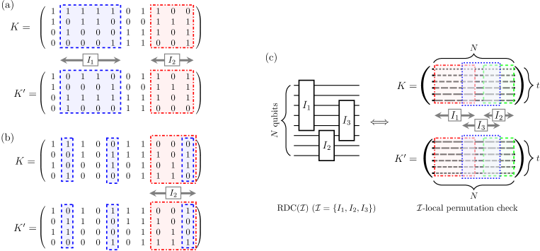
Figure 1: Panel (a) and (b) are examples of local permutation check problems for $t=4$ and $N=10$. In Panel (a), $K_{I_{1}}=\{1111,0110,1000,0001\}$ is a permutation of $K^{\prime}_{I_{1}}=\{0110,0001,1111,1000\}$ (blue dashed boxes). However, $K_{I_{2}}$ is not a permutation of $K^{\prime}_{I_{2}}$ (red dash-dotted boxes). Hence, $K$ is an $\{I_{1}\}$-local but not an $\{I_{2}\}$-local permutation of $K^{\prime}$, also implying that $K$ is not a row permutation of $K^{\prime}$. In Panel (b), $K$ is identical with $K^{\prime}$ except blue dashed boxes and is a $2$-local permutation of $K^{\prime}$. However, due to the columns in the blue dashed boxes, $K$ fails to be a $3$-local permutation of $K^{\prime}$. To observe this, compare e.g. $K_{I_{2}}$ and $K^{\prime}_{I_{2}}$ in red dash-dotted boxes. Panel (c) illustrates a relation between RDC$(\mathcal{I})$ and an $\mathcal{I}$-local permutation check problem. As diagonal gates acts on $I_{1}$, $I_{2}$ and $I_{3}$, we first check if $K$ is a $\{I_{1},I_{2},I_{3}\}$-local permutation of $K^{\prime}$. That is, we check the permutation relations between sets of rows in the red dash-dotted, green dotted, and blue dashed boxes. If $K$ is $\{I_{1},I_{2},I_{3}\}$-local but not a row permutation of $K^{\prime}$, then $\left\langle K,K^{\prime}\right|\mathbb{E}_{D^{Z}\sim{\sf RDC}(\mathcal{I})}[(D^{Z})^{\otimes t,t}]\left|K,K^{\prime}\right\rangle=1$ and otherwise $0$.

Let $K$ and $K^{\prime}$ be $t\times N$ matrices with elements in $\{0,1\}$. For given $s\in[1,t]$ and $I\subset[1,N]$, we denote a subsequence $(K_{s,m})_{m\in I}$ of the $s$th row of $K$ by $K_{s,I}$, and a set $\{K_{s,I}\}_{s\in[1,t]}$ of such subsequences over all $s$ by $K_{I}$. We use the same notation also for $K^{\prime}$. Let $\Omega$ be a canonical map that rearranges the subsequences $K_{I}$ in ascending order, where the subsequences are regarded as binary numbers. For $\mathcal{I}=\{I\}$, we say that $K$ is an $\mathcal{I}$-local permutation of $K^{\prime}$ if $\forall I\in\mathcal{I}$, $\Omega(K_{I})=\Omega(K^{\prime}_{I})$. In particular, we say $K$ is a row permutation of $K^{\prime}$ if $\Omega(K_{I})=\Omega(K^{\prime}_{I})$ for $I=[1,N]$, which simply implies that a set of rows of $K$ is a permutation of that of $K^{\prime}$. In the following, we denote by $\mathcal{I}_{r}$ a set of all subsets in $[1,N]$ with $r$ elements. Using this notation, we define local permutation check problems as follows.

Definition 11 (Local permutation check problems).

Let $K$ and $K^{\prime}$ be $t\times N$ matrices with elements in $\{0,1\}$. For a given $\mathcal{I}=\{I_{i}\}$ ($I_{i}\subset[1,N]$), the task of the $\mathcal{I}$-local permutation check problem is to count the number of pairs $(K,K^{\prime})$ such that $K$ is not a row permutation but an $\mathcal{I}$-local permutation of $K^{\prime}$. We denote the number of such pairs by $\Lambda(\mathcal{I})$. In particular, for $\mathcal{I}_{r}$, we call the problem an $r$-local permutation check problem and denote the number of pairs by $\Lambda_{r}$.

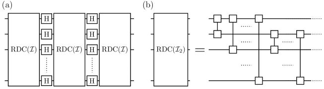
Figure 2: Panel (a) depicts iterations of RDC($\mathcal{I}$) and the Hadamard transformation. Panel (b) shows RDC($\mathcal{I}_{2})$, where random diagonal two-qubit gates are applied onto all pairs. The circuit is called RDC${}_{\rm disc}^{(t)}(\mathcal{I}_{2})$, when each two-qubit gate is replaced with $({\rm diag}_{Z}\{1,e^{i\varphi_{1}}\}\otimes{\rm diag}_{Z}\{1,e^{i\varphi_{2}}\}){\rm diag}_{Z}\{1,1,1,e^{i\vartheta}\}$, where the phases $\phi_{1},\phi_{2}$ and $\vartheta$ are chosen from discrete sets given in the main text.

For a couple of examples of local permutation checks, see Fig. 1. The following lemma provides the connection between the $\mathcal{I}$-local permutation check problem and implementations of quantum TPEs by RDC$(\mathcal{I})$ (see Appendix D for the proof).

Lemma 12.

Let $2^{N}=\Omega(t^{2}t!^{2})$. For a given $\mathcal{I}=\{I_{i}\}$ where $I_{i}\subset[1,N]$, iterating RDC$(\mathcal{I})$ and the Hadamard transformation $H_{N}$ on $N$ qubits, such as RDC$(\mathcal{I})H_{N}RDC(\mathcal{I})H_{N}RDC(\mathcal{I})$ (see Fig. 2 (a)), yields a quantum $(\tilde{\eta},t)$-TPE where

$$\tilde{\eta}\leq\eta+3t!\frac{\Lambda(\mathcal{I})}{2^{tN}}+\biggl{(}\frac{\Lambda(\mathcal{I})}{2^{tN}}\biggr{)}^{2}$$ (8)

with $\eta=\frac{(1+t^{2})t!^{2}+t^{2}}{2^{N}}+O(\frac{t^{4}t!^{2}}{2^{2N}})$.

To obtain our second main result, RDC$(\mathcal{I}_{2})$ (see Fig. 2 (b)) and the $2$-local permutation check problem are of particular importance. Due to the result in Ref. NKM2014 , we know that $\Lambda_{2}=0$ for $t\leq 3$. When $t\geq 4$, the problem can be rephrased as an extremal problem under dimension constraints, which is a constrained problem in extremal algebraic theory AAK2003 ; AAK2003-2 . By solving the problem, we obtain the following key lemma (see Sec. IV.3 for the proof).

Lemma 13.

For the $2$-local permutation check problem, it holds that $\Lambda_{2}\leq 2^{2t^{2}+(t-1)N}$.

It immediately follows from Lemmas 12 and 13 that, when $t=o(N^{1/2})$, iterating RDC$(\mathcal{I}_{2})$ and the Hadamard transformation is a quantum $(\tilde{\eta},t)$-TPE, where

$$\tilde{\eta}\leq 2^{2t^{2}+2-N}t!+O\bigl{(}t^{2}t!^{2}2^{-N}\bigr{)},$$ (9)

from which we obtain an efficient implementation of a unitary $t$-design due to Theorem 6. We can further reduce the number of randomness in the implementation by replacing all gates in RDC$(\mathcal{I}_{2})$ with those in the form of

$$\bigl{(}{\rm diag}\{1,e^{i\varphi_{1}}\}\otimes{\rm diag}\{1,e^{i\varphi_{2}}\}\bigr{)}{\rm diag}\{1,1,1,e^{i\vartheta}\}.$$ (10)

When $\varphi_{1}$ and $\varphi_{2}$ are chosen independently from $\{2\pi m/a:m\in[0,a-1]\}$ uniformly at random, and $\vartheta$ is chosen from $\{2\pi m/b:m\in[0,b-1]\}$, we denote the circuit RDC${}_{\rm disc}(\mathcal{I}_{2}:a,b)$. Using the same technique as in Ref. NKM2014 , we obtain the following lemma.

Lemma 14.

Let $a\geq t+1$ and $b\geq\lfloor t/2\rfloor+1$. Then, we have $\mathbb{E}[{\rm RDC}_{\rm disc}(\mathcal{I}_{2}:a,b)^{\otimes t,t}]=\mathbb{E}[{\rm RDC}(\mathcal{I}_{2})^{\otimes t,t}]$.

In particular, we denote RDC${}_{\rm disc}(\mathcal{I}_{2}:t+1,\lfloor t/2\rfloor+1)$ simply by RDC${}_{\rm disc}^{(t)}(\mathcal{I}_{2})$, where one two-qubit gate requires $2\log_{2}(t+1)+\log_{2}(\lfloor t/2\rfloor+1)<3\log_{2}(t+1)$ random bits. Together with all of these, we obtain our second main result.

Theorem 15.

(Main Result 2) Let $t=o(N^{1/2})$. Then, iterating RDC${}_{\rm disc}^{\ (t)}(\mathcal{I}_{2})$ and the Hadamard transformation on $N$ qubits such as $\bigl{(}RDC_{\rm disc}^{(t)}(\mathcal{I}_{2})H_{N}\bigr{)}^{2\ell}RDC_{\rm disc}^{(t)}(\mathcal{I}_{2})$ yields an $\epsilon$-approximate unitary $t$-design if

$$\ell\geq t+\frac{\log_{2}(1/\epsilon)}{N},$$ (11)

up to the leading order of $N$ and $t$. The total number of two-qubit gates and random bits are given by

$$\text{ \# of two-qubit gates }=\Theta\bigl{(}N\bigl{(}tN+\log_{2}(1/\epsilon)\bigr{)}\bigr{)},$$ (12)

$$\text{ \# of random bits }=\Theta\bigl{(}(\log_{2}t)N\bigl{(}tN+\log_{2}(1/\epsilon)\bigr{)}\bigr{)},$$ (13)

respectively.

	Total number of gates	$t$	Non-commuting depth NHMW2015-2
Classical tensor expanders HL2009TPE	poly$(N)$	$O(N/\log N))$	poly$(N)$
Local random circuits BHH2012	$O\bigl{(}t^{9}N(tN+\log(1/\epsilon))\bigr{)}$	poly$(N)$	$O\bigl{(}t^{9}(tN+\log(1/\epsilon))\bigr{)}$
Random diagonal circuits	$O\bigl{(}N(tN+\log_{2}(1/\epsilon))\bigr{)}$	$o(N^{1/2})$	$O\bigl{(}t+\frac{1}{N}\log_{2}(1/\epsilon)\bigr{)}$

Table 1: A comparison between quantum circuit constructions of unitary $t$-designs on $N$ qubits, which works for $t\geq 3$. The total number of quantum gates to achieve classical tensor expanders is known to be poly$(N)$, but is not explicitly presented in Ref. HL2009TPE . The non-commuting depth was introduced in Ref. NHMW2015-2 and is defined by the circuit depth when each commuting part of the circuit is counted as one step. The non-commuting depth may be of experimental importance.

Although we assume in Theorem 15 that $t=o(N^{1/2})$. However, we believe that Theorem 15 holds even for $t=o(N/\log N)$, which comes from the conjecture explained in more detail in Sec. IV.3.

In terms of $t$, Theorem 15 drastically improves the previous result using $O\bigl{(}t^{9}N(tN+\log(1/\epsilon))\bigr{)}$ two-qubit gates BHH2012 (see also Table 1 for the comparison) and is essentially optimal when the design is defined on a finite set of unitaries. This is because the support of a unitary $t$-design should contain at least $O(2^{2tN})$ unitaries RS2009 . Thus, when each gate in a random quantum circuit is chosen from a finite set, the scaling of the length necessary for the circuit achieving a $t$-design cannot be substantially better than linear in $t$.

In practical uses of unitary designs such as decoupling HaydenTutorial ; DBWR2010 ; SDTR2013 ; HM14 and randomised benchmarking EAZ2005 ; KLRetc2008 ; MGE2011 ; MGE2012 , unitary $2$-designs are known to be sufficient, which can be achieved more efficiently than our construction if one uses a Clifford circuit CLLW2015 . However, unitary $4$-designs are needed in a few applications S2005 ; BH2013 ; KRT2014 , which cannot be achieved by any Clifford circuit Z2015 . Moreover, higher-designs are generally more useful than lower-designs because they have stronger large deviation bounds L2009LDB , which are finite approximations of the concentration of measure for Haar random unitaries stating that values of any slowly varying function on a unitary group are likely to be almost constant if the dimension is large L2001 . This implies that using higher-designs in any applications of unitary designs results in better performance. As our implementation provides a shorter quantum circuit for $t$-designs than the existing ones HL2009 ; BHH2012 , it contributes to improve the performance of quantum protocols using unitary designs D2005 ; DW2004 ; GPW2005 ; ADHW2009 ; HaydenTutorial ; DBWR2010 ; SDTR2013 ; HM14 ; EAZ2005 ; KLRetc2008 ; MGE2011 ; MGE2012 ; S2005 ; BH2013 ; KRT2014 ; KL15 ; OAGKAL2016 .

This construction of approximate designs also has advantages from an experimental point of view. As highlighted in Ref. NHMW2015-1 ; NHMW2015-2 , the quantum circuits repeating RDC$(\mathcal{I}_{2})$ or RDC${}_{\rm disc}^{(t)}(\mathcal{I}_{2})$ and the Hadamard transformation are divided into a constant number of commuting parts. Indeed, only non-commuting parts are the Hadamard parts. Because the gates in each commuting part do not have any temporal order, they can be applied simultaneously in experimental realisations, making the implementations more robust. Hence, the commuting structure of our construction may help reducing the practical time and increasing the robustness of the implementations. This property can be rephrased in terms of the non-commuting depth proposed in Ref. NHMW2015-2 (see Table 1).

III.3 Hamiltonian dynamics and unitary designs

In the last decade, unitary designs were revealed to be the key to understanding fascinating phenomena in complex quantum many-body systems PSW2006 ; GLTZ2006 ; R2008 ; GE2016 ; HP2007 ; SS2008 ; S2011 ; LSHOH2013 ; S2014 ; HQRY2016 , in most of which the dynamics is assumed to be so random that it can be described by unitary designs. This assumption may be reasonable as a first approximation. However, due to the lack of full understanding of natural microscopic dynamics generating unitary designs, it is not clear to what extent the assumption can be justified. Most recently, the idea of scrambling was introduced in black hole information science HP2007 ; SS2008 . The main concern there is the fast scrambling conjecture, stating that the shortest time necessary for natural dynamics to scramble many-body systems scales logarithmically with the system size SS2008 ; S2011 ; LSHOH2013 ; S2014 ; HQRY2016 . While it is known that $0$-dimensional systems, where all particles interact with each other, can be scrambled in a constant time M2016 , the conjecture is strongly believed to hold in higher dimensions. The fast scrambling conjecture originally arises from a thought experiment concerning the black hole evaporation and the no-cloning theorem SS2008 , but has been also studied intensely in connection with quantum chaos SS2014 ; RD2015 ; SS2015 . So far, several inequivalent definitions of scrambling were proposed SS2008 ; LSHOH2013 ; HQRY2016 . Although they are useful for clarifying the relations between scrambling and other notions of randomisation such as unitary designs and the OTO correlators diagnosing quantum chaos SS2014 ; RD2015 ; SS2015 , there does not seem to be consensus on a rigorous mathematical definition of scrambling.

Here, we introduce design Hamiltonians as a unifying framework for studying randomising operations by physically natural Hamiltonian dynamics. In terms of the design Hamiltonians, we generalise the fast scrambling conjecture and propose a natural design Hamiltonian conjecture. We then construct a design Hamiltonian, where the interactions need to be changed only a few times before the corresponding time-evolution operators form unitary designs. This is in sharp contrast to the Hamiltonian dynamics based on local random quantum circuits BHH2012 , which will be elaborated on later.

We start with the definition of $k$-local Hamiltonians.

Definition 16 ($k$-local Hamiltonians KSV2002 ).

Let $\Lambda_{j}\subset[1,N]$ such that $|\Lambda_{j}|\leq k$ and $\Lambda_{i}\neq\Lambda_{j}$ if $i\neq j$. A $k$-local Hamiltonian $H$ on $N$ qubits is one in the form of $H=\sum_{i}H_{i}$, where each term $H_{i}$ may depend on time, acts non-trivially only on the qubits in $\Lambda_{i}$ and satisfies $|\!|H_{i}|\!|_{\infty}\leq 1$. We denote a set of all $k$-local Hamiltonians by $\mathfrak{H}_{k}$.

The interactions in $k$-local Hamiltonians are not necessarily geometrically local on lattice systems. They are rather interpreted as interactions on a given graph, where each vertex represents a particle. To normalise the time scale of the dynamics, we also assumed that the strength of each local interaction is bounded. In the following, to avoid confusion, we always use small $t$ and capital $T$ for $t$-designs and time, respectively. Denoting by $U_{H}(T):=\mathcal{T}\exp[-i\int_{0}^{T}dsH(s)]$, where $\mathcal{T}\exp$ is the time-ordered exponential, the time evolution operator at time $T$ generated by a possibly time-dependent Hamiltonian $H$, we now introduce a $t$-design Hamiltonian with $k$-local interactions as follows.

Definition 17 (An $\epsilon$-approximate $t$-design Hamiltonian with $k$-local interactions).

Let $\mathfrak{H}^{(t)}_{\epsilon}\subset\mathfrak{H}_{k}$ and ${\sf Ham}^{(t)}_{\epsilon}$ be a probability measure on $\mathfrak{H}^{(t)}_{\epsilon}$. If there exists $T_{0}>0$ such that, $\forall T\geq T_{0}$, a random unitary $U_{H}(T)$ generated by $H\sim{\sf Ham}^{(t)}_{\epsilon}$ is an $\epsilon$-approximate unitary $t$-design, the random Hamiltonian $H$ is called an $\epsilon$-approximate $t$-design Hamiltonian with $k$-local interactions. We also call the shortest such time $T_{0}$ a design time of $H$ .

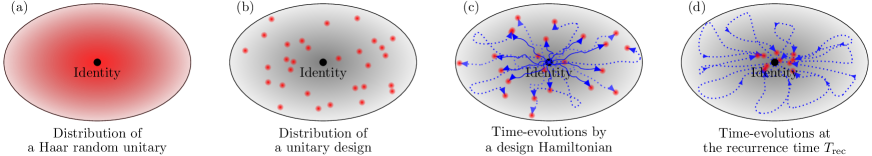
Figure 3: Schematic figures illustrating the distributions of random unitaries in a whole unitary group. For the visualisation, the unitary group is represented by an ellipse and each red dot corresponds to a unitary operator. Panel (a) illustrates a Haar random unitary, which is uniformly and continuously distributed over the whole unitary group. For unitary designs, the distribution is not necessarily continuous and is often defined on a finite support, which is depicted in Panel (b). Panel (c) provides an intuitive picture of time-evolution operators generated by a design Hamiltonian, starting from the identity. As time passes, a design Hamiltonian generates random unitary distributed over the whole unitary. The time evolution is illustrated by a trajectory in the panel. When the design Hamiltonian is defined on a finite ensemble of Hamiltonians, there exists a time $T_{\rm rec}$, where all time evolution operators are in the neighbourhood of the identity, due to the Poincaré recurrence theorem as depicted in Panel (d).

Note that, in this sense, there is no design Hamiltonian on a finite ensemble of time-independent Hamiltonians. Due to the Poincaré recurrence theorem BL1957 , the time-evolution operator generated by a time-independent Hamiltonian is in the neighbourhood of the identity operator at the recurrence time. Although the time-evolution operators generated by other Hamiltonians are possibly not the identity at the recurrence time of one Hamiltonian, we can always find the time $T_{\rm rec}$ where all operators are close to the identity. Hence, at that time, an ensemble of time-evolution operators does not form unitary designs (see also Fig. 3). However, this problem can be avoided if we consider time-dependent Hamiltonians or a continuous ensemble of time-independent Hamiltonians. We can also relax the condition of $\forall T\geq T_{0}$ to most of the time after $T_{0}$. For simplicity, in this paper, we define the design Hamiltonian as in Definition 17.

As our main purpose is to find physically natural Hamiltonians generating unitary designs, we are most interested in the design Hamiltonians which are not finely structured, are time-independent and are with geometrically local interactions. In addition, we may further require that, due to the fast scrambling conjecture, the design time scales logarithmically with the system size, which may depend on $t$. Thus, we arrive at the following conjecture.

Conjecture (Natural design Hamiltonian conjecture).

There exist $\epsilon$-approximate $t$-design Hamiltonians on $N$ qubits that satisfy the following three conditions:

1. the interactions are geometrically local,

2. the interactions are all time-independent,

3. the design time is given by $O(t\log N)$, which may also depend on $\epsilon$.

In general, the Hamiltonians with random interactions are expected to exhibit many-body localization SPA2013 ; HNO2014 ; NH2015 , preventing the corresponding dynamics from achieving unitary designs quickly. However, this is not always the case. For instance, the dynamics of a Majorana fermion model with random four-body interactions, also known as the Sachdev-Ye-Kitaev (YSK) model SY1993 ; K2015 is known to be strongly chaotic K2015Feb ; MSS2016 and is likely to achieve unitary designs at least on the low energy subspace. Although the SYK model consists of all-to-all interactions and does not meet the first condition of the conjecture, the further investigation of the model may help the search of natural design Hamiltonians satisfying all the three conditions.

The conjecture is based on an established language of unitary designs and so will be helpful to explore randomising operations in physically natural systems in a mathematically rigorous manner. We note that the conjecture is not only of theoretical interest but also of practical importance because, by applying such a random Hamiltonian onto a system, a unitary design will be spontaneously obtained. Most importantly, there is no need to change the interactions and no fine control of time is required. This will drastically simplify the implementations of unitary designs in experiments, also resulting in the simplification of many quantum protocols D2005 ; DW2004 ; GPW2005 ; ADHW2009 ; HaydenTutorial ; DBWR2010 ; SDTR2013 ; HM14 ; EAZ2005 ; KLRetc2008 ; MGE2011 ; MGE2012 ; S2005 ; BH2013 ; KRT2014 ; KL15 ; OAGKAL2016 .

The construction of designs by local random quantum circuits BHH2012 can be naturally translated into design Hamiltonians: a random Hamiltonian with neighbouring two-body interactions is a $t$-design Hamiltonian if the interactions vary randomly and independently at every time step. Such varying interactions can be considered to be fluctuations induced by white noise on two-body interactions OBKBWE2016 . This design Hamiltonian $H_{\rm rand}$ satisfies the first condition of the conjecture, as it uses only neighbouring interactions, but not the second and the third ones. Indeed, to achieve a unitary $t$-design by the dynamics of $H_{\rm rand}$, the interactions should be changed $O(t^{10}N)$ times uniformly at random. This is far from time-independent and takes much longer than $O(t\log N)$.

Here, we are more concerned with the second condition of the conjecture and provide a design Hamiltonian $H_{XZ}$ based on Theorem 15. We start with introducing a parameter set $\mathcal{P}_{t}(c)$ by

$$\mathcal{P}_{t}(c) =\biggl{\{}\frac{m}{2(\lfloor t/2\rfloor+1)}:m\in\bigl{[}-c,c\bigr{]}\biggr{\}}.$$ (14)

We then define finite sets of commuting Hamiltonians:

$$\mathfrak{H}_{Z}^{(t)} :=\biggl{\{}-\sum_{j<k}J_{ik}Z_{j}\otimes Z_{k}-\sum_{j}B_{j}Z_{j}\biggr{\}}_{J_{jk}\in\mathcal{P}_{t}(J),B_{j}\in\mathcal{P}_{t}(B)},$$ (15)

$$\mathfrak{H}_{X}^{(t)} :=\biggl{\{}-\sum_{j<k}J_{ik}X_{j}\otimes X_{k}-\sum_{j}B_{j}X_{j}\biggr{\}}_{J_{jk}\in\mathcal{P}_{t}(J),B_{j}\in\mathcal{P}_{t}(B)},$$ (16)

where $J=\frac{\lfloor t/2\rfloor}{2}$ and $B=\lfloor t/2\rfloor+\frac{1}{2}$. These types of disordered Hamiltonians are similar to those in many-body localised systems SPA2013 ; HNO2014 ; NH2015 , while interactions typically decay with increasing distance in such systems. Finally, we introduce a notation $\in_{\rm R}$ which implies that the left-hand side is drawn uniformly at random from the set in the right-hand side.

Figure 4: A schematic figure about the design Hamiltonian $H_{XZ}\in_{\rm R}\mathfrak{H}_{XZ}^{(t)}$. At each time interval $m$, $H_{Z}^{(m)}$ or $H_{X}^{(m)}$ is chosen uniformly at random from $\mathfrak{H}_{Z}^{(t)}$ or $\mathfrak{H}_{X}^{(t)}$, respectively. As depicted at the bottom of the figure, a random unitary generated by $H_{XZ}$ rapidly spreads over the whole unitary group and forms unitary designs in a short time independent of the system size.

Our third result is given as follows (see Sec. IV.4 for the proof).

Corollary 18 (Main result 3).

Let $t=o(N^{1/2})$ and $\mathfrak{H}_{XZ}^{(t)}$ be a set of $2$-local time-dependent Hamiltonians in the form of

$$H_{XZ}(T)=\begin{cases}H_{Z}^{(m)}&\text{if\ \ $2m\pi\leq T<(2m+1)\pi$},\\ H_{X}^{(m)}&\text{if\ \ $(2m+1)\pi\leq T<2(m+1)\pi$},\end{cases}$$ (17)

where $T$ denote time, and $H_{W}^{(m)}\in\mathfrak{H}_{W}^{(t)}$ for any $m=0,1,\cdots$ ($W=X,Z$). Then, the random Hamiltonian $H_{XZ}\in_{\rm R}\mathfrak{H}_{XZ}^{(t)}$ is an $\epsilon$-approximate $t$-design Hamiltonian. The design time of $H_{XZ}$ is at most $\bigl{(}2t+1+\frac{2}{N}\log_{2}(1/\epsilon)\bigr{)}\pi$.

Since $H_{XZ}$ is composed of $H_{Z}$ and $H_{X}$, both of which exhibit many-body localization, one may think that the time-evolution operators generated by $H_{XZ}\in_{\rm R}\mathfrak{H}_{XZ}^{(t)}$ shall not spread over the whole unitary group. However, due to the periodic change of the interaction basis, the localization indeed helps the time-evolution operators to be uniform. This can be observed from the fact that a random unitary diagonal in a fixed basis has a strong randomisation power when the initial state has a large support in that basis NTM2012 ; NakataThesis . Since a localized state in one basis has a large support in the complementary basis, the time-evolution by $H_{Z}$ ($H_{X}$) randomises the localized eigenstates of $H_{X}$ ($H_{Z}$) strongly. For this reason, it is natural to expect that the time-evolution operators generated by $H_{XZ}$ eventually form a unitary design, as rigorously proven in Corollary 18.

Note that our specific choice of the parameters in the Hamiltonians $H_{Z}$ and $H_{X}$, namely $J_{jk}\in_{\rm R}\mathcal{P}_{t}(J)$ and $B_{j}\in_{\rm R}\mathcal{P}_{t}(B)$, is to minimize the randomness needed to construct a design Hamiltonian. It is possible to choose the parameters from different sets as long as they are sufficiently random, where the design time will be accordingly changed. From a physical point of view, it may be interesting to consider physically feasible noises as parameter sets, which is in the same spirit as Ref. OBKBWE2016 .

Corollary 18 implies that the random Hamiltonian $H_{XZ}$ quickly generates the time evolution which can be hardly distinguished from completely random one (see also Fig. 4). Most notably, the design time is $O(t)$ and independent of the system size. As a simple consequence, any correlation functions at time $T$ in the system described by such a Hamiltonian quickly converges to the Haar averaged values. One of the important instances is the $2t$-point OTO correlator, which is expected to diagnose quantum chaos and has been studied in strongly correlated systems SS2014 ; RD2015 ; SS2015 . As the $2t$-point OTO correlators are polynomials of a unitary with degree $t$, their values in the system of a random Hamiltonian $H_{XZ}$ are $\epsilon$-close to the Haar random averages when $T\gtrsim(2t+1+\frac{2}{N}\log_{2}(1/\epsilon))\pi$. Furthermore, due to the large deviation bounds for unitary designs L2009LDB , this implies that almost any Hamiltonian in $\mathfrak{H}_{XZ}^{(t)}$ saturates the $2t$-point OTO correlators to the Haar random averages in a short time irrespective of the system size. As the OTO correlators are saturated in quantum chaotic systems HQRY2016 , our result indicates a close connection between the Hamiltonians in $\mathfrak{H}_{XZ}^{(t)}$ and quantum chaos, which suggests that the framework of design Hamiltonians may be useful to investigate the dynamics in quantum chaotic systems. This is also supported by a recently clarified relation between unitary designs and quantum chaos RB2016 .

Design Hamiltonian	Interactions	Time-dependence	Design time
$H_{\rm rand}$	Nearest neighbour interactions	Highly dependent	$O(t^{10}N)$
$H_{XZ}$	All-to-all two-body interactions	Nearly time-independent	$O(t)$

Table 2: A comparison of design Hamiltonians, $H_{\rm rand}$ BHH2012 and $H_{XZ}$, in terms of the three conditions of the natural design Hamiltonian conjecture. The design time of $H_{XZ}$ is much shorter than that of $H_{\rm rand}$ both in terms of $t$ and $N$. Although the improvement in terms of $t$ is generic to $H_{XZ}$, that in terms of $N$ is possibly due to its all-to-all interactions (see the main text).

In Table 2, we compare two design Hamiltonians $H_{\rm rand}$ and $H_{XZ}$. We emphasise that the design time $O(t)$ of $H_{XZ}$ is significantly faster than the design time $O(t^{10}N)$ of $H_{\rm rand}$ in terms of both $t$ and $N$. We should note, however, that although the improvement in terms of $t$ is intrinsic to $H_{XZ}$, the improvement in terms of $N$ may be rather due to the all-to-all interactions of $H_{XZ}$. Such interactions may naturally appear in cavity QED SM2002 ; GLG2011 ; SS2011 due to the cavity modes mediating long-range interactions, and unitary designs may possibly be realised in a short time. Nevertheless, for the fair comparison with $H_{\rm rand}$, the realisation of all-to-all interactions by neighbouring ones should be taken into account. This can be achieved if every particle travels all corners of the system and interacts with all the other particles, taking $O(N)$ time. Hence, when the interactions are neighbouring, the actual time for $H_{XZ}$ to achieve unitary designs is considered to be $O(tN)$, also implying that it does not violate the fast scrambling conjecture.

Unfortunately, both design Hamiltonians $H_{\rm rand}$ and $H_{XZ}$ do not satisfy all three conditions of the natural design Hamiltonian conjecture. However, we believe that existence of two design Hamiltonians $H_{\rm rand}$ and $H_{XZ}$, and previous analyses on the original fast scrambling conjecture SS2008 ; S2011 ; LSHOH2013 ; S2014 ; HQRY2016 provide substantial evidences for the natural design Hamiltonian conjecture.

IV Proofs

In this section, we provide proofs of theorems and lemmas given in Section III. We first introduce additional notation and useful lemmas in Subsection IV.1. The proof of our first main result, Theorem 9, is given in Subsection IV.2. We prove Lemma 13 in Subsection IV.3, which is the key lemma to obtain our second main result, and conclude this section by showing Corollary 18 about design Hamiltonians in Subsection IV.4.

IV.1 Additional notation and lemmas

Let $E=\{\left|k\right\rangle_{E}\}_{k\in[0,d-1]}$ and $F=\{\left|\alpha\right\rangle_{F}\}_{\alpha\in[0,d-1]}$ be orthogonal bases in $\mathcal{H}$. As we deal with $t$ copies of the Hilbert space, $\mathcal{H}^{\otimes t}$, we denote $[0,d-1]^{t}$ by $\mathcal{N}$ and introduce bases $\{\left|\mathbf{k}\right\rangle_{W}\}_{\mathbf{k}\in\mathcal{N}}$ ($W=E,F$) in $\mathcal{H}^{\otimes t}$, where $\left|\mathbf{k}\right\rangle_{W}=\bigotimes_{s=1}^{t}\left|{k_{s}}\right\rangle_{W}$, $\mathbf{k}=(k_{1},\cdots,k_{t})^{T}\in\mathcal{N}$, and $T$ represents the transpose. In the following, we always label the basis $E$ and $F$ by Latin and Greek alphabets, respectively, and do not write the subscript $E$ and $F$ explicitly.

Let $S_{t}$ be a permutation group of degree $t$. For $\pi\in S_{t}$, we denote $(k_{\pi^{-1}(1)},\cdots,k_{\pi^{-1}(t)})^{T}$ by $\mathbf{k}_{\pi}$, and define a state $\left|\Psi_{\pi}\right\rangle\in\mathcal{H}^{\otimes 2t}$ by

$$\left|\Psi_{\pi}\right\rangle :=I\otimes V(\pi)\left|\Phi\right\rangle$$ (18)

$$=\frac{1}{d^{t/2}}\sum_{\mathbf{k}\in\mathcal{N}}\left|\mathbf{k},{\mathbf{k}^{*}_{\pi}}\right\rangle$$ (19)

$$=\frac{1}{d^{t/2}}\sum_{\boldsymbol{\alpha}\in\mathcal{N}}\left|\boldsymbol{\alpha},{\boldsymbol{\alpha}^{*}_{\pi}}\right\rangle,$$ (20)

where $V(\pi)$ is a unitary representation of $\pi$, $\left|\Phi\right\rangle$ is the maximally entangled state between the first $\mathcal{H}^{\otimes t}$ and the second $\mathcal{H}^{\otimes t}$, $\left|\mathbf{k},{\mathbf{k}^{*}_{\pi}}\right\rangle=\left|\mathbf{k}\right\rangle\otimes(\left|\mathbf{k}_{\pi}\right\rangle)^{*}$ and $\left|\boldsymbol{\alpha},\boldsymbol{\alpha}^{*}_{\pi}\right\rangle=\left|\boldsymbol{\alpha}\right\rangle\otimes(\left|\boldsymbol{\alpha}_{\pi}\right\rangle)^{*}$. Note that $\left|\Psi_{\pi}\right\rangle$ and $\left|\Psi_{\sigma}\right\rangle$ are not necessarily orthogonal depending on the permutation element. We denote $\left|\Psi_{\pi}\right\rangle\left\langle\Psi_{\pi}\right|$ simply by $\Psi_{\pi}$.

We also introduce three subspaces in $\mathcal{H}^{\otimes 2t}$,

$$\mathcal{H}_{E}={\rm span}\{\left|\mathbf{k},\mathbf{k}^{*}_{\pi}\right\rangle:\mathbf{k}\in\mathcal{N},\pi\in S_{t}\},$$ (21)

$$\mathcal{H}_{F}={\rm span}\{\left|\boldsymbol{\alpha},\boldsymbol{\alpha}^{*}_{\pi}\right\rangle:\boldsymbol{\alpha}\in\mathcal{N},\pi\in S_{t}\},$$ (22)

$$\mathcal{H}_{0}={\rm span}\{\left|\Psi_{\pi}\right\rangle:\pi\in S_{t}\}.$$ (23)

Obviously, $\mathcal{H}_{E}\supsetneq\mathcal{H}_{0}$ and $\mathcal{H}_{F}\supsetneq\mathcal{H}_{0}$. The projectors onto the subspaces $\mathcal{H}_{E}$, $\mathcal{H}_{F}$ and $\mathcal{H}_{0}$ are denoted by $P_{E}$, $P_{F}$ and $P_{0}$, respectively. We further introduce an equivalent relation $\sim_{\boldsymbol{k}}$ ($\boldsymbol{k}\in\mathcal{N}$) in $S_{t}$ such that $\pi\sim_{\boldsymbol{k}}\sigma$ if and only if $\mathbf{k}_{\pi}=\mathbf{k}_{\sigma}$. A set of representative elements in equivalence classes by $\sim_{\boldsymbol{k}}$ is denoted by $S_{t}^{\mathbf{k}}$. Using this notation, the projectors $P_{E}$ and $P_{F}$ are explicitly given by

$$P_{E} =\sum_{\mathbf{k}\in\mathcal{N}}\sum_{\pi\in S^{\mathbf{k}}_{t}}\left|\mathbf{k},\mathbf{k}^{*}_{\pi}\right\rangle\left\langle\mathbf{k},\mathbf{k}^{*}_{\pi}\right|,$$ (24)

$$P_{F} =\sum_{\boldsymbol{\alpha}\in\mathcal{N}}\sum_{\pi\in S^{\boldsymbol{\alpha}}_{t}}\left|\boldsymbol{\alpha},\boldsymbol{\alpha}^{*}_{\pi}\right\rangle\left\langle\boldsymbol{\alpha},\boldsymbol{\alpha}^{*}_{\pi}\right|$$ (25)

We have the following lemmas for these projectors.

Lemma 19 (Ref. BHH2012 ; NKM2014 ).

For Haar random unitaries $U$, random diagonal-unitaries $D^{E}$ in the basis of $E$, and those $D^{F}$ in the basis of $F$, the following hold

$$\mathbb{E}_{U\sim{\sf H}}[U^{\otimes t,t}]=P_{0},$$ (26)

$$\mathbb{E}_{D^{E}\sim{\sf D}_{E}}[(D^{E})^{\otimes t,t}]=P_{E},$$ (27)

$$\mathbb{E}_{D^{F}\sim{\sf D}_{F}}[(D^{F})^{\otimes t,t}]=P_{F}.$$ (28)

Lemma 20 (Ref. BHH2012 ).

It holds that $|\!|P_{0}-\sum_{\pi\in S_{t}}\Psi_{\pi}|\!|_{\infty}\leq\frac{t^{2}}{d}$.

IV.2 Proof of Theorem 9

We now prove Theorem 9. Due to the independence of random diagonal unitaries $D^{E}$, $D^{\prime E}$ and $D^{F}$ and Lemma 19, we have

$$|\!|\mathbb{E}_{D^{E},D^{\prime E}\sim{\sf D}_{E},D^{F}\sim{\sf D}_{F}}[(D^{E}D^{F}D^{\prime E})^{\otimes t,t}]-\mathbb{E}_{U\sim{\sf H}}[U^{\otimes t,t}]|\!|_{\infty}=|\!|P_{E}P_{F}P_{E}-P_{0}|\!|_{\infty},$$ (29)

which is bounded from above as follows:

$$|\!|P_{E}P_{F}P_{E}-P_{0}|\!|_{\infty} \leq|\!|P_{E}P_{F}P_{E}-\sum_{\pi\in S_{t}}\Psi_{\pi}|\!|_{\infty}+|\!|P_{0}-\sum_{\pi\in S_{t}}\Psi_{\pi}|\!|_{\infty}$$ (30)

$$\leq|\!|P_{E}(P_{F}-\sum_{\pi\in S_{t}}\Psi_{\pi})P_{E}|\!|_{\infty}+\frac{t^{2}}{d},$$ (31)

where we have used the triangular inequality in the first line, the fact that $\left|\Psi_{\pi}\right\rangle\in\mathcal{H}_{0}\subset\mathcal{H}_{E}$ and Lemma 20 in the second line. Using the fact that the operator norm for Hermitian operators is bounded from above by the row norm, defined by $\max_{j}\sum_{i}|A_{ij}|$ for an Hermitian operator $A$, we have

$$|\!|\mathbb{E}_{D^{E},D^{\prime E}\sim{\sf D}_{E},D^{F}\sim{\sf D}_{F}}[(D^{E}D^{F}D^{\prime E})^{\otimes t,t}]-\mathbb{E}_{U\sim{\sf H}}[U^{\otimes t,t}]|\!|_{\infty} \leq C,$$ (32)

where

$$C=\max_{\mathbf{l}\in\mathcal{N}}\max_{\sigma\in S_{t}^{\mathbf{l}}}\sum_{\mathbf{k}\in\mathcal{N}}\sum_{\chi\in S_{t}^{\mathbf{k}}}\bigl{|}\left\langle\mathbf{l},\mathbf{l}^{*}_{\sigma}\right|P_{F}-\sum_{\pi\in S_{t}}\Psi_{\pi}\left|\mathbf{k},\mathbf{k}^{*}_{\chi}\right\rangle\bigr{|}+\frac{t^{2}}{d}.$$ (33)

Note that it suffices to consider only vectors in $\mathcal{H}_{E}^{\otimes t,t}$ when we compute the first term of Eq. (31), which is because the operator is sandwiched by the projector $P_{E}$. In the following, we evaluate $C$.

Substituting $\left|\Psi_{\pi}\right\rangle=\frac{1}{\sqrt{d^{t}}}\sum_{\mathbf{m}\in\mathcal{N}}\left|\mathbf{m},\mathbf{m}^{*}_{\pi}\right\rangle$, the second term is given by

$$\left\langle\mathbf{l},\mathbf{l}^{*}_{\sigma}\right|\sum_{\pi\in S_{t}}\Psi_{\pi}\left|\mathbf{k},\mathbf{k}^{*}_{\chi}\right\rangle =\frac{1}{d^{t}}\sum_{\pi\in S_{t}}\delta_{\mathbf{l}_{\pi},\mathbf{l}_{\sigma}}\delta_{\mathbf{k}_{\pi},\mathbf{k}_{\chi}}.$$ (34)

On the other hand, using an explicit form of $P_{F}$ given in Eq. (25), the first term can be expanded to be

$$\left\langle\mathbf{l},\mathbf{l}^{*}_{\sigma}\right|P_{F}\left|\mathbf{k},\mathbf{k}^{*}_{\chi}\right\rangle =\sum_{\boldsymbol{\alpha}\in\mathcal{N}}\sum_{\pi\in S_{t}^{\boldsymbol{\alpha}}}\left\langle\mathbf{l}|\boldsymbol{\alpha}\right\rangle\left\langle\boldsymbol{\alpha}|\mathbf{k}\right\rangle\left\langle\mathbf{k}_{\pi^{-1}\circ\chi}|\boldsymbol{\alpha}\right\rangle\left\langle\boldsymbol{\alpha}|\mathbf{l}_{\pi^{-1}\circ\sigma}\right\rangle.$$ (35)

Since a pair of the bases $(E,F)$ is a Fourier-type pair, it satisfies for any $l,k,\alpha\in[0,d-1]$ that $\left\langle l|\alpha\right\rangle\left\langle k|\alpha\right\rangle=\left\langle l+k|\alpha\right\rangle/d^{1/2}$, where $l+k\in[0,d-1]$ as $[0,d-1]$ is an additive group with respect to $+$ . Denoting $(l_{1}+k_{1},\cdots,l_{t}+k_{t})^{T}$ by $\mathbf{l}+\mathbf{k}$, we have

$$\left\langle\mathbf{l},\mathbf{l}_{\sigma}^{*}\right|P_{F}\left|\mathbf{k},\mathbf{k}_{\chi}^{*}\right\rangle =\frac{1}{d^{t}}\sum_{\boldsymbol{\alpha}\in\mathcal{N}}\sum_{\pi\in S_{t}^{\boldsymbol{\alpha}}}\left\langle\mathbf{l}+\mathbf{k}_{\pi^{-1}\circ\chi}|\boldsymbol{\alpha}\right\rangle\left\langle\boldsymbol{\alpha}|\mathbf{k}+\mathbf{l}_{\pi^{-1}\circ\sigma}\right\rangle$$ (36)

$$=\frac{1}{d^{t}}\sum_{\boldsymbol{\alpha}\in\mathcal{N}}\biggl{(}\sum_{\pi\in S_{t}}-\sum_{\pi\in S_{t}\setminus S_{t}^{\boldsymbol{\alpha}}}\biggr{)}\left\langle\mathbf{l}+\mathbf{k}_{\pi^{-1}\circ\chi}|\boldsymbol{\alpha}\right\rangle\left\langle\boldsymbol{\alpha}|\mathbf{k}+\mathbf{l}_{\pi^{-1}\circ\sigma}\right\rangle$$ (37)

$$=\frac{1}{d^{t}}\biggl{(}\sum_{\pi\in S_{t}}\delta_{\mathbf{l}+\mathbf{k}_{\pi^{-1}\circ\chi},\mathbf{k}+\mathbf{l}_{\pi^{-1}\circ\sigma}}-M_{\mathbf{l},\mathbf{k}}\biggr{)},$$ (38)

where $M_{\mathbf{l},\mathbf{k}}=\sum_{\boldsymbol{\alpha}\in\mathcal{N}}\sum_{\pi\in S_{t}\setminus S_{t}^{\boldsymbol{\alpha}}}\left\langle\mathbf{l}+\mathbf{k}_{\pi^{-1}\circ\chi}|\boldsymbol{\alpha}\right\rangle\left\langle\boldsymbol{\alpha}|\mathbf{k}+\mathbf{l}_{\pi^{-1}\circ\sigma}\right\rangle$, and we used $\sum_{\boldsymbol{\alpha}\in\mathcal{N}}\left|\boldsymbol{\alpha}\right\rangle\left\langle\boldsymbol{\alpha}\right|=I_{\mathcal{H}^{\otimes t}}$. Hence, using the triangular inequality, we obtain

$$|\left\langle\mathbf{l},\mathbf{l}_{\sigma}^{*}\right|P_{F}-\sum_{\pi\in S_{t}}\Psi_{\pi}\left|\mathbf{k},\mathbf{k}_{\chi}^{*}\right\rangle| =\frac{1}{d^{t}}\biggl{|}\sum_{\pi\in S_{t}}\bigl{(}\delta_{\mathbf{l}+\mathbf{k}_{\pi^{-1}\circ\chi},\mathbf{k}+\mathbf{l}_{\pi^{-1}\circ\sigma}}-\delta_{\mathbf{l}_{\pi},\mathbf{l}_{\sigma}}\delta_{\mathbf{k}_{\pi},\mathbf{k}_{\chi}}\bigr{)}-M_{\mathbf{l},\mathbf{k}}\biggr{|}$$ (39)

$$\leq\frac{1}{d^{t}}\biggl{|}\sum_{\pi\in S_{t}}\bigl{(}\delta_{\mathbf{l}+\mathbf{k}_{\pi^{-1}\circ\chi},\mathbf{k}+\mathbf{l}_{\pi^{-1}\circ\sigma}}-\delta_{\mathbf{l}_{\pi},\mathbf{l}_{\sigma}}\delta_{\mathbf{k}_{\pi},\mathbf{k}_{\chi}}\bigr{)}\biggr{|}+\frac{1}{d^{t}}\bigl{|}M_{\mathbf{l},\mathbf{k}}\bigr{|}.$$ (40)

An upper bound of $|M_{\mathbf{l},\mathbf{k}}\bigr{|}$ can be obtained from the fact that the bases $E$ and $F$ are mutually unbiased, leading to

$$\bigl{|}M_{\mathbf{l},\mathbf{k}}\bigr{|}\leq\frac{1}{d^{t}}\sum_{\boldsymbol{\alpha}\in\mathcal{N}}|S_{t}\setminus S_{t}^{\boldsymbol{\alpha}}|.$$ (41)

As $|S_{t}\setminus S_{t}^{\boldsymbol{\alpha}}|$ depends only on how many different elements $\boldsymbol{\alpha}$ contains, the number of which we denote by $k$, and the number of every different element $\alpha_{i}$ in $\boldsymbol{\alpha}$, denoted by $s_{i}$, we replace the summation with that over $k$ and obtain

$$\sum_{\boldsymbol{\alpha}\in\mathcal{N}}\bigl{|}S_{t}\setminus S_{t}^{\boldsymbol{\alpha}}\bigr{|}=\sum_{k=1}^{t}\binom{d}{k}g^{(k)}(t),$$ (42)

where the binomial coefficient counts the number of possible choices of $k$ different numbers from $[0,d-1]$, and $g^{(k)}(t)$ is the function that depends only on $k$ and $t$ given by

$$g^{(k)}(t)=\sum_{(s_{1},\cdots,s_{k})}\frac{t!}{s_{1}!\cdots s_{k}!}\bigl{(}t!-\frac{t!}{s_{1}!\cdots s_{k}!}\bigr{)}.$$ (43)

Here, the summation is taken over all possible $(s_{1},\cdots,s_{k})$ such that $\forall i\in[1,k]$ $s_{i}\in[1,t]$ and $\sum_{i=1}^{k}s_{i}=t$. For a fixed $k$, the number of such combinations is simply given by $\binom{t-1}{k-1}$. For $k=t$, $s_{i}=1$ for all $i\in[1,k]$ and thus $g^{(t)}(t)=0$. For the remaining terms $g^{(k)}(t)$ ($k\in[1,t-1]$), we use an upper bound given by

$$g^{(k)}(t)\leq\binom{t-1}{k-1}\frac{t!^{2}}{4},$$ (44)

which is optimal when $k=t-1$. Substituting these, we obtain

$$\sum_{\boldsymbol{\alpha}\in\mathcal{N}}\bigl{|}S_{t}\setminus S_{t}^{\boldsymbol{\alpha}}\bigr{|} \leq\frac{t!^{2}}{4}\sum_{k=1}^{t-1}\binom{d}{k}\binom{t-1}{k-1}$$ (45)

$$=\frac{t!^{2}}{4}\biggl{(}\binom{d-1+t}{t}-\binom{d}{t}\biggr{)},$$ (46)

where the last line is obtained due to the Vandermonde’s identity. Since $d=\Omega(t^{2})$, an upper bound is obtained such as

$$\sum_{\boldsymbol{\alpha}\in\mathcal{N}}\bigl{|}S_{t}\setminus S_{t}^{\boldsymbol{\alpha}}\bigr{|} \leq t^{2}t!d^{t-1}+O(t^{4}t!d^{t-2}),$$ (47)

which leads to

$$|\left\langle\mathbf{l},\mathbf{l}^{*}_{\sigma}\right|P_{F}-\sum_{\pi\in S_{t}}\Psi_{\pi}\left|\mathbf{k},\mathbf{k}^{*}_{\chi}\right\rangle| \leq\frac{1}{d^{t}}\biggl{|}\sum_{\pi\in S_{t}}\bigl{(}\delta_{\mathbf{l}+\mathbf{k}_{\pi^{-1}\circ\chi},\mathbf{k}+\mathbf{l}_{\pi^{-1}\circ\sigma}}-\delta_{\mathbf{l}_{\pi},\mathbf{l}_{\sigma}}\delta_{\mathbf{k}_{\pi},\mathbf{k}_{\chi}}\bigr{)}\biggr{|}+\frac{t^{2}t!}{d^{t+1}}+O\biggl{(}\frac{t^{4}t!}{d^{t+2}}\biggr{)}.$$ (48)

Substituting this into $C$, the following upper bound can be obtained:

$$C \leq\frac{t^{2}(t!^{2}+1)}{d}+\frac{1}{d^{t}}\max_{\mathbf{l}\in\mathcal{N}}\max_{\sigma\in S_{t}^{\mathbf{l}}}\sum_{\mathbf{k}\in\mathcal{N}}\sum_{\chi\in S_{t}^{\mathbf{k}}}\biggl{|}\sum_{\pi\in S_{t}}\bigl{(}\delta_{\mathbf{l}+\mathbf{k}_{\pi^{-1}\circ\chi},\mathbf{k}+\mathbf{l}_{\pi^{-1}\circ\sigma}}-\delta_{\mathbf{l}_{\pi},\mathbf{l}_{\sigma}}\delta_{\mathbf{k}_{\pi},\mathbf{k}_{\chi}}\bigr{)}\biggr{|}+O\biggl{(}\frac{t^{4}t!^{2}}{d^{2}}\biggr{)}$$ (49)

$$=\frac{t^{2}(t!^{2}+1)}{d}+\frac{1}{d^{t}}\max_{\mathbf{l}\in\mathcal{N}}\max_{\sigma\in S_{t}^{\mathbf{l}}}\sum_{\mathbf{k}\in\mathcal{N}}\sum_{\chi\in S_{t}^{\mathbf{k}}}\sum_{\pi\in S_{t}}\bigl{(}\delta_{\mathbf{l}+\mathbf{k}_{\pi^{-1}\circ\chi},\mathbf{k}+\mathbf{l}_{\pi^{-1}\circ\sigma}}-\delta_{\mathbf{l}_{\pi},\mathbf{l}_{\sigma}}\delta_{\mathbf{k}_{\pi},\mathbf{k}_{\chi}}\bigr{)}+O\biggl{(}\frac{t^{4}t!^{2}}{d^{2}}\biggr{)}$$ (50)

$$\leq\frac{t^{2}(t!^{2}+1)}{d}+\frac{1}{d^{t}}\max_{\mathbf{l}\in\mathcal{N}}\max_{\sigma\in S_{t}^{\mathbf{l}}}\sum_{\pi\in S_{t}}\sum_{\mathbf{k}\in\mathcal{N}}\sum_{\chi(\neq\pi)\in S_{t}^{\mathbf{k}}}\delta_{\mathbf{l}+\mathbf{k}_{\pi^{-1}\circ\chi},\mathbf{k}+\mathbf{l}_{\pi^{-1}\circ\sigma}}+O\biggl{(}\frac{t^{4}t!^{2}}{d^{2}}\biggr{)}$$ (51)

$$\leq\frac{t^{2}(t!^{2}+1)}{d}+\frac{1}{d^{t}}\max_{\mathbf{l}\in\mathcal{N}}\max_{\sigma\in S_{t}^{\mathbf{l}}}\sum_{\pi\in S_{t}}\sum_{\chi(\neq\pi)\in S_{t}}\sum_{\mathbf{k}\in\mathcal{N}}\delta_{\mathbf{l}+\mathbf{k}_{\pi^{-1}\circ\chi},\mathbf{k}+\mathbf{l}_{\pi^{-1}\circ\sigma}}+O\biggl{(}\frac{t^{4}t!^{2}}{d^{2}}\biggr{)},$$ (52)

where the second line is due to a fact that the term in the modulus is non-negative because, when the second term is one, the first term is also one, the third line is obtained by using a fact that the first and the second term cancel each other when $\chi=\pi$ and by dropping negative terms when $\chi\neq\pi$, and the last line is due to $S_{t}^{\mathbf{k}}\subset S_{t}$. For the delta function $\delta_{\mathbf{l}+\mathbf{k}_{\pi^{-1}\circ\chi},\mathbf{k}+\mathbf{l}_{\pi^{-1}\circ\sigma}}$, we have

$$\delta_{\mathbf{l}+\mathbf{k}_{\pi^{-1}\circ\chi},\mathbf{k}+\mathbf{l}_{\pi^{-1}\circ\sigma}}=1\Longleftrightarrow\forall s\in[1,t],\ \ \ \ l_{s}+k_{\chi^{-1}\circ\pi(s)}=k_{s}+l_{\sigma^{-1}\circ\pi(s)}$$ (53)

When $\chi\neq\pi$, there exists at least one pair $(s,s^{\prime})$ ($s\neq s^{\prime}\in[1,t]$) such that $\pi(s)=\chi(s^{\prime})$. Hence, $k_{s^{\prime}}=k_{s}+l_{\sigma^{-1}\circ\pi(s)}-l_{s}$ should be at least satisfied for the delta function to be non-zero. Thus, the number of $\mathbf{k}$, for which the delta function is non-zero, is at most $d^{t-1}$. Based on this observation, we obtain

$$\max_{\mathbf{l}\in\mathcal{N}}\max_{\sigma\in S_{t}^{\mathbf{l}}}\sum_{\pi\in S_{t}}\sum_{\chi(\neq\pi)\in S_{t}}\sum_{\mathbf{k}\in\mathcal{N}}\delta_{\mathbf{l}+\mathbf{k}_{\pi^{-1}\circ\chi},\mathbf{k}+\mathbf{l}_{\pi^{-1}\circ\sigma}}\leq t!^{2}d^{t-1}.$$ (54)

Substituting this into Eq. (52), we obtain an upper bound of $C$, leading to

$$|\!|\mathbb{E}_{D^{E},D^{\prime E}\sim{\sf D}_{E},D^{F}\sim{\sf D}_{F}}[(D^{E}D^{F}D^{\prime E})^{\otimes t,t}]-\mathbb{E}_{U\sim{\sf H}}[U^{\otimes t,t}]|\!|_{\infty}\leq\frac{(1+t^{2})t!^{2}+t^{2}}{d}+O\biggl{(}\frac{t^{4}t!^{2}}{d^{2}}\biggr{)}.$$ (55)

This concludes the proof. $\hfill\blacksquare$

IV.3 Proof of Lemma 13

We first provide a key lemma to prove Lemma 13. The lemma is seen as a constrained problem in extremal algebraic theory AAK2003 ; AAK2003-2 . The proof is given in Appendix E.

Lemma 21.

Let $O$ be an orthogonal matrix acting on the Euclidean space $\mathbb{R}^{t}$, which contains the set of apexes of a hypercube, $\{0,1\}^{t}$. If there exists a set $S\subset\{0,1\}^{t}$ such that $OS\subset\{0,1\}^{t}$ and $|S|>2^{t-1}$, then $O$ is a permutation matrix.

Now, we prove Lemma 13, i.e. $\Lambda_{2}=|L_{2}|\leq 2^{2t^{2}+(t-1)N}$. Here, $L_{2}$ is the set of pairs $(K,K^{\prime})$, where $K$ is a $2$-local but not a row permutation of $K^{\prime}$.

Proof (Lemma 13).

Throughout the proof, we denote the column vectors of $K$ and $K^{\prime}$ by $\vec{k}_{i}$ and $\vec{k}^{\prime}_{i}$, respectively, for $i\in[1,N]$. The $2$-local permutation condition is equivalent to the following:

$$\forall i,j\in[1,N],\ \ \vec{k}_{i}\cdot\vec{k}_{j}=\vec{k}^{\prime}_{i}\cdot\vec{k}^{\prime}_{j},$$ (56)

where $\cdot$ is the usual Euclidean inner product. This is because the conditions for $i=j$ imply that the number of $1$’s in $\vec{k}_{i}$ and that in $\vec{k}^{\prime}_{i}$ should be the same, and those for $i\neq j$ imply that the number of $11$ in $K_{\{i,j\}}$ is equal to that in $K^{\prime}_{\{i,j\}}$. These conditions together correspond to the necessary and sufficient conditions for the pair $(K,K^{\prime})$ to be $2$-local permutations. Moreover, Eq. (56) implies that the Gram matrix of a set $\{\vec{k}_{i}:i\in[1,N]\}$ of column vectors is the same as that of $\{\vec{k}^{\prime}_{i}:i\in[1,N]\}$. Hence, ${\rm span}\{\vec{k}_{i}:i\in[1,N]\}$ has the same dimension as ${\rm span}\{\vec{k}^{\prime}_{i}:i\in[1,N]\}$. It also follows that there exists a partial isometry $O$ that satisfies $O\vec{k}_{i}=\vec{k}^{\prime}_{i}$ for any $i\in[1,N]$, i.e. $OK=K^{\prime}$. If the partial isometry is restricted to its support, it is an orthogonal matrix as the elements of the vectors are in $\{0,1\}$, and it is not a permutation operator due to the assumption that $K$ is not a row permutation of $K^{\prime}$.

We will now construct a set $\mathcal{O}$ of orthogonal matrices on $\mathbb{R}^{t}$ that satisfies

$$\forall(K,K^{\prime})\in L_{2},\exists O\in\mathcal{O}\text{\ such that\ }OK=K^{\prime}.$$ (57)

This can be done as follows. Let $s:=2^{2t}$ and $[0,s-1]^{\leq t}$ be the set of $s$-ary strings of length $t$ or smaller. We describe a procedure of defining a set $S_{2}\subset[0,s-1]^{\leq t}$ and orthogonal matrices $O_{\bf{b}}$ for $\mathbf{b}\in S_{2}$, such that $S_{2}$ is a prefix code and that $\mathcal{O}:=\{O_{\mathbf{b}}|\mathbf{b}\in S_{2}\}$ satisfies Eq. (57). Our construction starts with $S_{2}=\emptyset$ and is recursive in terms of the rank $\kappa$ of the partial isometry obtained from $(K,K^{\prime})$. We repeat the subroutine described below from $\kappa=t$ to $\kappa=1$ by decreasing $\kappa$ one by one. In the subroutine, we first choose $(K,K^{\prime})\in L_{2}$ that defines a partial isometry with rank $\kappa$. We pick up an arbitrary set of independent column vectors $\{\vec{k}_{i_{m}}\}_{m=1}^{\kappa}$ in $K$ and those $\{\vec{k}^{\prime}_{i_{m}}\}_{m=1}^{\kappa}$ in $K^{\prime}$. These vectors can be converted to an $s$-ary string $\mathbf{b}=(2^{t}k_{i_{1}}+k^{\prime}_{i_{1}},2^{t}k_{i_{2}}+k^{\prime}_{i_{2}},\cdots,2^{t}k_{i_{\kappa}}+k^{\prime}_{i_{\kappa}})$ of length $\kappa$ by regarding each vector as a binary number with length $t$. If $\mathbf{b}$ is a prefix of a string $\mathbf{b}^{\prime}\in S_{2}$, then the orthogonal matrix $O_{\mathbf{b}^{\prime}}$ satisfies $O_{\mathbf{b}^{\prime}}K=K^{\prime}$ because, on the support of the partial isometry obtained from $(K,K^{\prime})$, the action of $O_{\mathbf{b}^{\prime}}$ is the same as that of the isometry by construction. Otherwise, we append $\mathbf{b}$ to $S_{2}$, and define an orthogonal matrix $O_{\mathbf{b}}$ as an arbitrary extension of the partial isometry. The subroutine is run for all $(K,K^{\prime})\in L_{2}$ with a partial isometry of rank $\kappa$. Eventually, we obtain a set $\mathcal{O}$ of orthogonal matrices on $\mathbb{R}^{t}$. Importantly, it does not contain a permutation matrix and, by construction, $|\mathcal{O}|=|S_{2}|\leq 2^{2t^{2}}$.

Introducing a set $L_{2}(O)$ by $\{(K,OK):K,OK\in\{0,1\}^{tN}\}$ for a given orthogonal matrix $O\in\mathbb{R}^{t}$, we have $L_{2}\subset\bigcup_{O\in\mathcal{O}}L_{2}(O)$, leading to

$$\Lambda_{2} \leq\sum_{O\in\mathcal{O}}|L_{2}(O)|$$ (58)

$$\leq|\mathcal{O}|\max_{O\in\mathcal{O}}|L_{2}(O)|$$ (59)

$$\leq 2^{2t^{2}}\max_{O\in\mathcal{O}}|L_{2}(O)|.$$ (60)

Since the condition $OK\in\{0,1\}^{tN}$ consists of an identical and independent condition on each column of $K$, $|L_{2}(O)|$ for $O\in\mathcal{O}$ is bounded from above by

$$|L_{2}(O)|\leq\biggl{(}\max_{O\in\mathcal{O}}\bigl{|}\{\vec{k}\in\{0,1\}^{t}:O\vec{k}\in\{0,1\}^{t}\}\bigr{|}\biggr{)}^{N}.$$ (61)

As $O\in\mathcal{O}$ is on $\mathbb{R}^{t}$ and is not a permutation matrix, from the contraposition of Lemma 21, we obtain

$$\max_{O\in\mathcal{O}}\bigl{|}\{\vec{k}\in\{0,1\}^{t}:O\vec{k}\in\{0,1\}^{t}\bigr{|}\leq 2^{t-1}.$$ (62)

Thus, we have $\Lambda_{2}\leq 2^{2t^{2}+(t-1)N}$, and conclude the proof. $\hfill\blacksquare$

Finally, we note that the upper bound given in Lemma 13 is unlikely to be tight in terms of $t$ because an upper bound $|\mathcal{O}|$ given by $2^{2t^{2}}$ in the proof is far from optimal. This is observed from the fact that $|\mathcal{O}|=|S_{2}|$ but $S_{2}$ does not contain all strings with length $t$. More concretely, we provide instances for a small $t$. From the result in Ref. NKM2014 , we know that, for any pair $(K,K^{\prime})$, $K$ is a row permutation of $K^{\prime}$ if and only if $K$ is a $(\lfloor\log_{2}t\rfloor+1)$-local permutation of $K^{\prime}$. Hence, the smallest $t$ making the $2$-local permutation check problem non-trivial is $4$. In this case, we can show that, if $K$ is a $2$-local but not a row permutation of $K^{\prime}$, the four rows of $K$ and those of $K^{\prime}$ can be rearranged independently, resulting in $K_{\pi}$ and $K^{\prime}_{\sigma}$ respectively ($\pi,\sigma\in S_{4}$), such that a pair of the $i$th column of $K_{\pi}$ and that of $K^{\prime}_{\sigma}$ are in the set $C_{0}\cup C_{1}$ ($\forall i\in[1,N]$), where

$$C_{0} =\bigl{\{}\bigl{(}(0,0,0,0)^{T},(0,0,0,0)^{T}\bigr{)},\bigl{(}(1,1,1,1)^{T},(1,1,1,1)^{T}\bigr{)},\bigl{(}(0,0,1,1)^{T},(0,0,1,1)^{T}\bigr{)},$$

$$\ \ \ \ \ \ \ \ \bigl{(}(1,1,0,0)^{T},(1,1,0,0)^{T}\bigr{)},\bigl{(}(1,0,1,0)^{T},(1,0,1,0)^{T}\bigr{)},\bigl{(}(0,1,0,1)^{T},(0,1,0,1)^{T}\bigr{)}\bigr{\}},$$ (63)

$$C_{1} =\bigl{\{}\bigl{(}(0,1,1,0)^{T},(1,0,0,1)^{T}\bigr{)},\bigl{(}(1,0,0,1)^{T},(0,1,1,0)^{T}\bigr{)}\bigr{\}}.$$ (64)

Taking the number of choices of $\pi$ and $\sigma$ into account, we have

$$\Lambda_{2}<t!^{2}\bigl{(}|C_{0}|+|C_{1}|\bigr{)}^{N}=t!^{2}8^{N},$$ (65)

which corresponds to $t!^{2}2^{(t-1)N}$ for $t=4$. For this reason, we conjecture that the optimal bound should be given by $f(t)2^{(t-1)N}$ where $f(t)=O({\rm poly}(t!))$, which we have analytically confirmed for $t\leq 7$. If this conjecture is true, Theorem 15 works for $t=o(N/\log N)$ instead of $t=o(N^{1/2})$.

IV.4 Proof of Corollary 18

We prove Corollary 18 that, $\forall T\geq(2t+1+\frac{2}{N}\log_{2}1/\epsilon)\pi$, a random unitary $U_{XZ}(T)=\mathcal{T}\exp[-i\int_{0}^{T}dsH_{XZ}(s)]$ generated by $H_{XZ}(T)\in_{\rm R}\mathfrak{H}_{XZ}^{(t)}$ at time $T$ is an $\epsilon$-approximate unitary $t$-design, where $\mathfrak{H}_{XZ}^{(t)}$ is the set of Hamiltonians in the form of Eq. (17).

Proof (Corollary 18).

In the proof, we denote $e^{-i\tau H_{W}^{(m)}}$ by $U_{W}^{(m)}(\tau)$ ($W=X,Z$). As both Hamiltonians are composed of commuting terms, they are simply given by

$$e^{-i\tau H_{X}^{(m)}}=\prod_{k<k^{\prime}}e^{i\tau J_{kk^{\prime}}^{(m)}X_{k}\otimes X_{k^{\prime}}}\prod_{k}e^{i\tau B_{k}^{(m)}X_{k}}\ \ \ {\rm and}\ \ \ e^{-i\tau H_{Z}^{(m)}}=\prod_{k<k^{\prime}}e^{i\tau\tilde{J}_{kk^{\prime}}^{(m)}Z_{k}\otimes Z_{k^{\prime}}}\prod_{k}e^{i\tau\tilde{B}_{k}^{(m)}Z_{k}}.$$ (66)

We first consider a random unitary $U_{XZ}(T_{\ell})$ at time $T_{\ell}=(2\ell+1)\pi$ ($\ell=1,2,\dots$). Using the above notation, it is given by

$$U_{XZ}(T_{\ell})=U_{Z}^{(\ell+1)}(\pi)\prod_{m=\ell}^{1}U_{X}^{(m)}(\pi)U_{Z}^{(m)}(\pi).$$ (67)

We take the average of $U_{XZ}(T_{\ell})^{\otimes t,t}$ over $H_{XZ}\in_{\rm R}\mathfrak{H}_{XZ}^{(t)}$, which is equivalent to take the average over all parameters $B_{k}^{(m)},\tilde{B}_{k^{\prime}}^{(m)}\in_{\rm R}\mathcal{P}_{t}(B)$ and $J_{kk^{\prime}}^{(m)},\tilde{J}_{kk^{\prime}}^{(m)}\in_{\rm R}\mathcal{P}_{t}(J)$. Here, the parameter set $\mathcal{P}_{t}(c)$ is given by Eq. (14) such as

$$\mathcal{P}_{t}(c) =\biggl{\{}\frac{m}{2(\lfloor t/2\rfloor+1)}:m\in\bigl{[}-c,c\bigr{]}\biggr{\}},$$ (68)

and $(B,J)=(\lfloor t/2\rfloor+1/2,\lfloor t/2\rfloor/2)$. Since it holds that

$$e^{i\pi J_{kk^{\prime}}^{(m)}Z_{k}\otimes Z_{k^{\prime}}}\ e^{i\pi B_{k}^{(m)}Z_{k}}\otimes e^{i\pi B_{k^{\prime}}^{(m)}Z_{k^{\prime}}}\\ =e^{\pi i(J_{kk^{\prime}}^{(m)}+B_{k}^{(m)}+B_{k^{\prime}}^{(m)})}\bigl{(}{\rm diag}_{Z}\{1,e^{-2\pi i(J_{kk^{\prime}}^{(m)}+B_{k^{\prime}}^{(m)})}\}\otimes{\rm diag}_{Z}\{1,e^{-2\pi i(J_{kk^{\prime}}^{(m)}+B_{k}^{(m)})}\}\bigr{)}{\rm diag}_{Z}\{1,1,1,e^{4\pi iJ_{kk^{\prime}}^{(m)}}\},$$ (69)

if $B_{k}^{(m)},B_{k^{\prime}}^{(m)}\in_{\rm R}\mathcal{B}_{t}$ and $J_{kk^{\prime}}^{(m)}\in_{\rm R}\mathcal{J}_{t}$, where

$$\mathcal{B}_{t} =\biggl{\{}\frac{m}{2(\lfloor t/2\rfloor+1)}:m\in[0,2\lfloor t/2\rfloor+1]\biggr{\}}$$ (70)

$$\mathcal{J}_{t} =\biggl{\{}\frac{m}{2(\lfloor t/2\rfloor+1)}:m\in[0,\lfloor t/2\rfloor]\biggr{\}},$$ (71)

then the probability distribution of $(-2\pi(J_{kk^{\prime}}^{(m)}+B_{k^{\prime}}),-2\pi(J_{kk^{\prime}}^{(m)}+B_{k}^{(m)}),4\pi J_{kk^{\prime}}^{(m)})$ is identical to that of $(\varphi,\varphi^{\prime},\theta)$ in Eq. (10) with $a=2(\lfloor t/2\rfloor+1)$ and $b=\lfloor t/2\rfloor+1$, implying that $U_{Z}^{(m)}(T_{\ell})$ is equivalent to ${\rm RDC}_{\rm disc}(\mathcal{I}_{2}:2b,b)$ up to a global phase. Noting that the global phase is cancelled in $U_{Z}^{(m)}(T_{\ell})^{\otimes t,t}$ and recalling that $\mathbb{E}[{\rm RDC}_{\rm disc}(\mathcal{I}_{2}:a,b)^{\otimes t,t}]=\mathbb{E}[{\rm RDC}(\mathcal{I}_{2})^{\otimes t,t}]$ if $a\geq t+1$ and $b\geq\lfloor t/2\rfloor+1$, we have

$$\mathbb{E}_{B_{k}^{(m)}\in_{\rm R}\mathcal{B}_{t},J_{kk^{\prime}}^{(m)}\in_{\rm R}\mathcal{J}_{t}}[U_{Z}^{(m)}(T_{\ell})^{\otimes t,t}]=\mathbb{E}[{\rm RDC}(\mathcal{I}_{2})^{\otimes t,t}].$$ (72)

Using a product of two-qubit diagonal gates $V$ given by

$$V=\bigotimes_{k=1}^{N}{\rm diag}_{Z}^{(k)}\{1,e^{2\pi i\Delta B}\}\bigotimes_{k<k^{\prime}}{\rm diag}_{Z}^{(kk^{\prime})}\{1,1,1,e^{-4\pi i\Delta J}\},$$ (73)

where the superscript of ${\rm diag}_{Z}$, such as $(k)$ and $(kk’)$, indicates the place of qubits the gate acts on, and $(\Delta B,\Delta J)=(\frac{\lfloor t/2\rfloor+1/2}{2(\lfloor t/2\rfloor+1)},\frac{\lfloor t/2\rfloor}{4(\lfloor t/2\rfloor+1)})$, we obtain

$$\mathbb{E}_{B_{k}^{(m)}\in_{\rm R}\mathcal{P}_{t}(B),J_{kk^{\prime}}^{(m)}\in_{\rm R}\mathcal{P}_{t}(J)}[U_{Z}^{(m)}(T_{\ell})^{\otimes t,t}] =\mathbb{E}_{B_{k}^{(m)}\in_{\rm R}\mathcal{B}_{t},J_{kk^{\prime}}^{(m)}\in_{\rm R}\mathcal{J}_{t}}[U_{Z}^{(m)}(T_{\ell})^{\otimes t,t}]V^{\otimes t,t}$$ (74)

$$=\mathbb{E}[{\rm RDC}(\mathcal{I}_{2})^{\otimes t,t}]V^{\otimes t,t},$$ (75)

where we used Eq. (72) in the last line. Further, because ${\rm RDC}(\mathcal{I}_{2})$ is composed of two-qubit diagonal gates with random phases uniformly drawn from $[0,2\pi)$, the average of ${\rm RDC}(\mathcal{I}_{2})^{\otimes t,t}$ does not change even when additional diagonal two-qubit gates are applied. Thus, we obtain

$$\mathbb{E}_{B_{k}^{(m)}\in_{\rm R}\mathcal{P}_{t}(B),J_{kk^{\prime}}^{(m)}\in_{\rm R}\mathcal{P}_{t}(J)}[U_{Z}^{(m)}(T_{\ell})^{\otimes t,t}]=\mathbb{E}[{\rm RDC}(\mathcal{I}_{2})^{\otimes t,t}].$$ (76)

As a similar relation holds for $X$ Hamiltonians, we conclude that

$$\mathbb{E}[U_{XZ}(T_{\ell})^{\otimes t,t}]=\mathbb{E}[\bigl{(}(RDC(\mathcal{I}_{2})H_{N})^{2\ell}RDC(\mathcal{I}_{2})\bigr{)}^{\otimes t,t}],$$ (77)

where $H_{N}$ is the Hadamard transformation on $N$ qubits, implying that $U_{XZ}(T_{\ell})$ is an $\epsilon$-approximate unitary $t$-design if $\ell\geq t+\frac{1}{N}\log_{2}(1/\epsilon)$.

To complete the proof, consider the time $T$ satisfying $T_{\ell}<T<T_{\ell+1}$ where $\ell\geq t+\frac{1}{N}\log_{2}(1/\epsilon)$. Because the time evolution operator from time $T_{\ell}$ to time $T$ is independent of the one before $T_{\ell}$, it follows from Lemma 4 that $U_{XZ}(T)$ is also an $\epsilon$-approximate unitary $t$-design. $\hfill\blacksquare$

V Conclusion and discussions

In this paper, we have presented new constructions of unitary $t$-designs and proposed design Hamiltonians as a general framework to investigate randomising operations in complex quantum many-body systems. The new constructions are based on repetitions of random diagonal-unitaries in mutually unbiased bases. We have first shown that, if the bases are Fourier-type, approximate unitary $t$-designs can be achieved on one qudit after $O(t)$ repetitions. We have then constructed quantum circuits on $N$ qubits that achieve approximate unitary $t$-designs using $O(tN^{2})$ gates, which drastically improves the previous result BHH2012 in terms of $t$. The dependence on $t$ is essentially optimal amongst designs with finite supports. The circuits were obtained by solving a special case of combinatorial problems, which we call the local permutation check problems, showing an interesting connection between combinatorics and efficient implementations of designs. Based on these results, we have provided a design Hamiltonian, which changes the interactions only a few times to generate designs. This result supports the natural design Hamiltonian conjecture and is also practically important as it simplifies the experimental implementations of unitary designs.

Our approach of studying unitary designs and randomising operations in physically natural systems opens a lot of interesting questions. The following are a few questions concerning unitary designs:

1. In one-qudit systems, is it possible to implement unitary $t$-designs by repeating random diagonal-unitaries in any non-trivial pairs of bases? If so, how many repetitions are sufficient for the implementations?

2. What is the best strategy of the local permutation check problems?

3. What is the most efficient implementation by quantum circuits that approximate random diagonal-unitaries in the Pauli-$Z$ basis?

4. What are the further applications of unitary $t$-designs for $t\geq 4$.

Regarding the question 1, we have found that repeating random diagonal-unitaries in non-trivial pairs of bases achieves a unitary $1$-design if any vector in one basis is not orthogonal to any vector in the other basis. Although this non-orthogonality condition may not be necessary, we expect that, for arbitrary non-trivial pairs of bases satisfying the non-orthogonality condition, the process eventually achieves unitary $t$-designs. The questions 2 and 3 are related each other due to Lemma 12. In this paper, we have considered only $2$-local permutation check problems. However, if there exists a set $\mathcal{I}=\{I\}$ such that $\Lambda(\mathcal{I})=O(2^{(t-1)N})$ and $|I|=$ constant for all $I\in\mathcal{I}$, then we can implement approximate unitary $t$-designs using $O(t|\mathcal{I}|)$ quantum gates. Hence, finding a better strategy for the local permutation check problems immediately results in a faster implementation of unitary designs. It is also desirable to directly search efficient quantum circuits approximating random diagonal-unitaries in the $Z$ basis because Lemma 12 may not be tight. Finally, it is important to find applications of unitary $t$-designs for large $t$. A possible and promising direction is to further explore large deviation bounds for unitary designs as mentioned in Section III.2.

We also list a few open questions about design Hamiltonians from the physical point of view:

1. Prove or disprove the natural design Hamiltonian conjecture.

2. What are the exact relations between natural design Hamiltonians and various definitions of scrambling or OTO correlators?

3. If a design Hamiltonian is defined on a finite ensemble of local Hamiltonians, how many Hamiltonians are needed?

4. What are the static features of design Hamiltonians such as thermal or quantum phases?

The question I is the most interesting one, where we could use the methods developed in the random matrix theory M1990 . A natural candidate of design Hamiltonians satisfying all the three conditions of the conjecture may be $H_{\rm localGUE}=\sum_{\langle i,j\rangle}h_{ij}$ where each local term $h_{ij}$ is drawn randomly and independently from the so-called Gaussian unitary ensemble M1990 and the summation is taken over all neighbouring qubits. We expect that $H_{\rm localGUE}$ generates a unitary design after some time although it may also be possible that it does not due to the many-body localization. The question II is important to clarify the roles of design Hamiltonians in black hole information science and quantum chaos. As design Hamiltonians are based on unitary designs, it suffices to investigate explicit relations between unitary designs and scrambling or the OTO correlators. The relation between unitary designs and the OTO correlators is recently addressed and is clarified in Ref. RB2016 . The question III is not only of theoretical interest but also of practical importance because it determines the number of random bits necessary to construct design Hamiltonians. To address this question, it is needed to relax the definition of design Hamiltonians to exclude the Poincaré recurrence time as we have mentioned in Section III.3. Note that, since the support of unitary $t$-designs on $N$ qubits should contain at least $O(2^{2tN})$ unitaries RS2009 , the ensemble should contain at least the same number of Hamiltonians. Finally, as design Hamiltonians are certain types of disordered Hamiltonians, it is natural to expect that they have special static properties, which is the question IV. A static property of the above random Hamiltonian $H_{\rm localGUE}$ was numerically studied from the viewpoint of distributions in a state space, and evidences of phase transitions were obtained NO2014 . However, as $H_{\rm localGUE}$ is not yet shown to be a design Hamiltonian and no time-independent design Hamiltonians have been found yet, it would be more realistic to start with investigating static properties of the Hamiltonian $H_{Z}$ of $H_{XZ}$, which has similarity to many-body localised systems, and their dependence on $t$.

VI Acknowledgements

The authors are grateful to S. Di Martino, C. Morgan and T. Sasaki for helpful discussions. The authors also thank B. Yoshida for fruitful discussions and for telling us recent progresses on scrambling and quantum chaos, and C. Gogolin for pointing out the possibility of using our construction for quantum metrology. This work is supported by CREST, JST, Grant No. JPMJCR1671. YN is a JSPS Research Fellow and is supported by JSPS KAKENHI Grant Number 272650. AW and CH are supported by the Spanish MINECO, Projects No. FIS2013-40627-P and No. FIS2016-80681-P, and CH by FPI Grant No. BES-2014-068888, as well as by the Generalitat de Catalunya, CIRIT project no. 2014 SGR 966. AW is further supported by the European Commission (STREP “RAQUEL”), the European Research Council (Advanced Grant “IRQUAT”).

Appendix A Proof of Lemma 4

Here, a simple proof of Lemma 4 is given.

Proof.

As an $\epsilon$-approximate unitary $t$-design $U$ satisfies $|\!|\mathcal{G}^{(t)}_{U\sim\nu}-\mathcal{G}^{(t)}_{U\sim{\sf H}}|\!|_{\diamond}\leq\epsilon$, we have

$$|\!|\mathcal{G}^{(t)}_{V}\circ\mathcal{G}^{(t)}_{U\sim\nu}-\mathcal{G}^{(t)}_{U\sim{\sf H}}|\!|_{\diamond} =|\!|\mathcal{G}^{(t)}_{V}\circ(\mathcal{G}^{(t)}_{U\sim\nu}-\mathcal{G}^{(t)}_{U\sim{\sf H}})|\!|_{\diamond}$$ (78)

$$\leq|\!|\mathcal{G}^{(t)}_{V}|\!|_{\diamond}|\!|\mathcal{G}^{(t)}_{U\sim\nu}-\mathcal{G}^{(t)}_{U\sim{\sf H}}|\!|_{\diamond}$$ (79)

$$\leq\epsilon,$$ (80)

where we used the unitary invariance of the Haar measure in the first line, and a fact that $\mathcal{G}^{(t)}_{V}$ is a completely-positive and trace-preserving map in the last line. This implies that $VU$ is also an $\epsilon$-approximate unitary $t$-design. The proof for $UV$ is similarly obtained.$\hfill\blacksquare$

Appendix B Proof of Theorem 6

Here, we provide a proof of Theorem 6, which follows almost directly from the following simple lemma.

Lemma 22.

For any unitary $U$, it holds that $U^{\otimes t,t}=P_{0}+(I-P_{0})U^{\otimes t,t}(I-P_{0})$.

Proof.

Using $\left|\Psi_{\pi}\right\rangle=I\otimes V(\pi)\left|\Phi\right\rangle$, we have for any $\pi\in S_{t}$ that

$$U^{\otimes t,t}\left|\Psi_{\pi}\right\rangle =U^{\otimes t}\otimes U^{*\otimes t}V(\pi)\left|\Phi\right\rangle$$ (81)

$$=U^{\otimes t}\otimes V(\pi)U^{*\otimes t}\left|\Phi\right\rangle$$ (82)

$$=U^{\otimes t}U^{\dagger\otimes t}\otimes V(\pi)\left|\Phi\right\rangle$$ (83)

$$=I\otimes V(\pi)\left|\Phi\right\rangle$$ (84)

$$=\left|\Psi_{\pi}\right\rangle,$$ (85)

where we have used the fact that $U^{*\otimes t}$ commutes with $V(\pi)$ in the second line and the property of the maximally entangled state in the third line. This implies that $(I-P_{0})U^{\otimes t,t}P_{0}=0$. Replacing $U$ with $U^{\dagger}$ in Eq. (85), we also have $(I-P_{0})U^{\dagger\otimes t,t}P_{0}=0$, implying $P_{0}U^{\otimes t,t}(I-P_{0})=0$. Hence, we obtain $U^{\otimes t,t}=P_{0}+(I-P_{0})U^{\otimes t,t}(I-P_{0})$. $\hfill\blacksquare$

Proof (Theorem 6).

To prove Theorem 6, let $\nu$ be a quantum $(\eta,t)$-TPE, satisfying

$$|\!|\mathbb{E}_{U\sim\nu}[U^{\otimes t,t}]-\mathbb{E}_{U\sim{\sf H}}[U^{\otimes t,t}]|\!|_{\infty}\leq\eta.$$ (86)

Applying Lemma 22 to all the unitaries in $\mathbb{E}_{U\sim\nu}[U^{\otimes t,t}]$, we have

$$\mathbb{E}_{U\sim\nu}[U^{\otimes t,t}]=P_{0}+(I-P_{0})\mathbb{E}_{U\sim\nu}[U^{\otimes t,t}](I-P_{0}).$$ (87)

Due to Lemma 19, which reads $P_{0}=\mathbb{E}_{U\sim{\sf H}}[U^{\otimes t,t}]$, the quantum TPE $\nu$ satisfies that

$$|\!|(I-P_{0})\mathbb{E}_{U\sim\nu}[U^{\otimes t,t}](I-P_{0})|\!|_{\infty}\leq\eta.$$ (88)

Let $\nu^{\ell}$ be a measure corresponding to that of the $\ell$ iterations of the quantum TPE $\nu$. Then,

$$|\!|\mathcal{G}^{(t)}_{U\sim\nu^{\ell}}-\mathcal{G}^{(t)}_{U\sim{\sf H}}|\!|_{\diamond} \leq d^{t}|\!|\mathcal{G}^{(t)}_{U\sim\nu^{\ell}}-\mathcal{G}^{(t)}_{U\sim{\sf H}}|\!|_{2\rightarrow 2}$$ (89)

$$=d^{t}|\!|\mathbb{E}_{U\sim\nu^{\ell}}[U^{\otimes t,t}]-\mathbb{E}_{U\sim{\sf H}}[U^{\otimes t,t}]|\!|_{\infty}$$ (90)

$$=d^{t}|\!|\bigl{(}\mathbb{E}_{U\sim\nu}[U^{\otimes t,t}]\bigr{)}^{\ell}-\mathbb{E}_{U\sim{\sf H}}[U^{\otimes t,t}]|\!|_{\infty}$$ (91)

$$=d^{t}|\!|\bigl{(}(I-P_{0})\mathbb{E}_{U\sim\nu}[U^{\otimes t,t}](I-P_{0})\bigr{)}^{\ell}|\!|_{\infty}$$ (92)

$$\leq d^{t}|\!|(I-P_{0})\mathbb{E}_{U\sim\nu}[U^{\otimes t,t}](I-P_{0})|\!|_{\infty}^{\ell}$$ (93)

$$\leq d^{t}\eta^{\ell}.$$ (94)

Here, the first line is due to the inequality that $|\!|\mathcal{E}|\!|_{\diamond}\leq D|\!|\mathcal{E}|\!|_{2\rightarrow 2}$ for any superoperators $\mathcal{E}$ acting on a $D$-dimensional system, the third line is obtained due to the independence of the measure of each iteration, the fourth line is from Eq. (87), and the last line is from Eq. (88). This implies that $\ell$ iterations of a quantum $(\eta,t)$-TPE is an $\epsilon$-approximate unitary $t$-design if $d^{t}\eta^{\ell}\leq\epsilon$. $\hfill\blacksquare$

Appendix C Proof of Lemma 8

Here, we prove Lemma 8 about the Fourier-type bases.

Proof (Lemma 8).

When a pair of two bases is that of arbitrary basis and its Fourier basis, it is clear that $\theta_{k\alpha}=\frac{2\pi k\alpha}{d}$ and the additive operation in the index is given by an addition modulo $d$. It can be easily checked that $[0,d-1]$ is an additive group with respect to the modular addition.

When the pair is given by the Pauli-$X$ and -$Z$ bases, using the binary representation such as $\alpha=\alpha_{1}\cdots\alpha_{N}$ $(\forall j\in[1,N],\alpha_{j}\in\{0,1\})$, the Pauli-$X$ and -$Z$ bases can be represented by

$$\left|\alpha\right\rangle_{X}=\bigotimes_{j=1}^{N}\left|\alpha_{j}\right\rangle_{X},\ \ \ \ \ \ \left|k\right\rangle_{Z}=\bigotimes_{j=1}^{N}\left|k_{j}\right\rangle_{Z},$$ (95)

respectively. Using a fact that ${}_{Z}\!\left\langle k_{j}|\alpha_{j}\right\rangle_{X}={}_{X}\!\left\langle\alpha_{j}|k_{j}\right\rangle_{Z}$ is equal t to $1/\sqrt{2}$ if $(\alpha_{j},k_{j})=(0,0),(0,1),(1,0)$ and is equal to $-1/\sqrt{2}$ if $(\alpha_{j},k_{j})=(1,1)$, we have $\theta_{k\alpha}=\pi\sum_{j=1}^{N}\delta_{k_{j}1}\delta_{\alpha_{j}1}$, leading to

$$\exp\bigl{[}i(\theta_{k\alpha}+\theta_{l\alpha})\bigr{]} =\exp\bigl{[}i\pi\sum_{j=1}^{N}(\delta_{k_{j}1}+\delta_{l_{j}1})\delta_{\alpha_{j}1}\bigr{]}$$ (96)

$$=\exp\bigl{[}i\pi\sum_{j=1}^{N}\delta_{k_{j}+l_{j},1}\delta_{\alpha_{j}1}\bigr{]}$$ (97)

$$=\exp\bigl{[}i\theta_{k\oplus l,\alpha}\bigr{]},$$ (98)

where $\oplus$ is a bitwise XOR, defined by $a\oplus b=0$ when $a=b$ and otherwise $1$ for binary numbers $a$ and $b$, and is the additive operation in the index, making $[0,d-1]$ an additive group. $\hfill\blacksquare$

Appendix D Proof of Lemma 12

Here, we prove Lemma 12 which connects the achievability of quantum-TPE with random diagonal circuits and the local permutation check problem.

Proof (Lemma 12).

Let ${\sf RDC}(\mathcal{I})$ be the probability measure of RDC$(\mathcal{I})$. We denote the averaged operators $\mathbb{E}_{D^{Z}\sim{\sf RDC}(\mathcal{I})}[(D^{Z})^{\otimes t,t}]$ and $\mathbb{E}_{D^{Z}\sim{\sf D}_{Z}}[(D^{Z})^{\otimes t,t}]$ by $Q_{Z}$ and $P_{Z}$, respectively. There exists a projector $R_{Z}$ diagonal in the Pauli-$Z$ basis such that $Q_{Z}=P_{Z}+R_{Z}$ because $Q_{Z}P_{Z}=P_{Z}Q_{Z}=P_{Z}$ and $Q_{Z}$ is a projector diagonal in the Pauli-$Z$ basis. Denoting $H_{N}^{\otimes t,t}Q_{Z}H_{N}^{\otimes t,t}$ by $Q_{X}$, where $H_{N}:=H^{\otimes N}$ is the Hadamard transformation on $N$ qubits, and similarly decomposing it into $P_{X}+R_{X}$ ($P_{X}:=H_{N}^{\otimes t,t}P_{Z}H_{N}^{\otimes t,t}$ and $R_{X}:=H_{N}^{\otimes t,t}R_{Z}H_{N}^{\otimes t,t}$), we have

$$|\!|Q_{Z}Q_{X}Q_{Z}-P_{0}|\!|_{\infty} =|\!|P_{Z}P_{X}P_{Z}-P_{0}+R_{Z}P_{X}P_{Z}+Q_{Z}P_{X}R_{Z}+Q_{Z}R_{X}P_{Z}+Q_{Z}R_{X}R_{Z}|\!|_{\infty}$$ (99)

$$\leq|\!|P_{Z}P_{X}P_{Z}-P_{0}|\!|_{\infty}+2|\!|P_{X}R_{Z}|\!|_{\infty}+|\!|R_{X}P_{Z}|\!|_{\infty}+|\!|R_{X}R_{Z}|\!|_{\infty}$$ (100)

$$\leq\eta+2|\!|P_{X}R_{Z}|\!|_{\infty}+|\!|R_{X}P_{Z}|\!|_{\infty}+|\!|R_{X}R_{Z}|\!|_{\infty},$$ (101)

where we used Theorem 9 in the last line.

We denote by $\mathcal{W}_{Z}$ a set of $(\mathbf{k}_{1},\mathbf{k}_{2})\in\mathcal{N}\times\mathcal{N}$ such that $\left\langle\mathbf{k}_{1},\mathbf{k}_{2}\right|R_{Z}\left|\mathbf{k}_{1},\mathbf{k}_{2}\right\rangle=1$. Using an upper bound of the operator norm by the row norm and using the fact that $|\left\langle\mathbf{l}_{1},\mathbf{l}_{2}\right|P_{X}\left|\mathbf{k}_{1},\mathbf{k}_{2}\right\rangle|=(\mathrm{tr}P_{X})/2^{2tN}\leq t!/2^{tN}$ for any $(\mathbf{k}_{1},\mathbf{k}_{2})$ and $(\mathbf{l}_{1},\mathbf{l}_{2})$, we obtain

$$|\!|R_{X}P_{Z}|\!|_{\infty}=|\!|P_{X}R_{Z}|\!|_{\infty}\leq\max_{(\mathbf{l}_{1},\mathbf{l}_{2})\in\mathcal{W}_{Z}}\sum_{(\mathbf{k}_{1},\mathbf{k}_{2})\in\mathcal{W}_{Z}}\biggl{|}\left\langle\mathbf{l}_{1},\mathbf{l}_{2}\right|P_{X}\left|\mathbf{k}_{1},\mathbf{k}_{2}\right\rangle\biggr{|}\leq\frac{t!}{2^{tN}}|\mathcal{W}_{Z}|.$$ (102)

Similarly, we have

$$|\!|R_{X}R_{Z}|\!|_{\infty} \leq\max_{(\mathbf{l}_{1},\mathbf{l}_{2})\in\mathcal{W}_{Z}}\sum_{(\mathbf{k}_{1},\mathbf{k}_{2})\in\mathcal{W}_{Z}}\biggl{|}\left\langle\mathbf{l}_{1},\mathbf{l}_{2}\right|R_{X}\left|\mathbf{k}_{1},\mathbf{k}_{2}\right\rangle\biggr{|}\leq\biggl{(}\frac{|\mathcal{W}_{Z}|}{2^{tN}}\biggr{)}^{2}.$$ (103)

Substituting Eqs. (102) and  (103) into Eq. (101), we obtain

$$|\!|Q_{Z}Q_{X}Q_{Z}-P_{0}|\!|_{\infty} \leq\eta+3t!\frac{|\mathcal{W}_{Z}|}{2^{tN}}+\biggl{(}\frac{|\mathcal{W}_{Z}|}{2^{tN}}\biggr{)}^{2}.$$ (104)

We finally show that $|\mathcal{W}_{Z}|=\Lambda(\mathcal{I})$. Note that $\Lambda(\mathcal{I})$ is the number of $(K,K^{\prime})\in\{0,1\}^{tN}\times\{0,1\}^{tN}$ such that $K$ is not a row permutation but is an $\mathcal{I}$-local permutation of $K^{\prime}$. We first express each $k_{s}\in\mathbf{k}$ in binary such as $k_{s}=k_{s1}\cdots k_{sN}$ and define a $t\times N$ matrix $K$ with elements in $\{0,1\}$ corresponding to $\mathbf{k}$,

$$K:=\begin{pmatrix}k_{11}&k_{12}&\cdots&k_{1N}\\ \vdots&\vdots&\ddots&\vdots\\ k_{t1}&k_{t2}&\cdots&k_{tN}\\ \end{pmatrix},$$ (105)

where $k_{sm}\in\{0,1\}$. Using this notation and noting that the $Z$-basis is real, the state $\left|\mathbf{k},\mathbf{k}^{\prime*}\right\rangle$ is expressed as $\left|K,K^{\prime}\right\rangle$. A random diagonal gate in RDC$(\mathcal{I})$ applied on qubits in $I\in\mathcal{I}$ corresponds to, after taking the tensor product and the average, an projector onto ${\rm span}\{\left|K,K^{\prime}\right\rangle:\Omega(K_{I})=\Omega(K^{\prime}_{I})\}$, where $\Omega$ is a canonical map that rearranges $|I|$-bit sequences $\{K_{s,I}\}_{s\in[1,t]}$ in ascending order. Thus, we have

$$\left\langle K,K^{\prime}\right|Q_{Z}\left|K,K^{\prime}\right\rangle=\begin{cases}1&\text{if $\forall I\in\mathcal{I}$, $\Omega(K_{I})=\Omega(K^{\prime}_{I})$},\\ 0&\text{otherwise}.\end{cases}$$ (106)

Note that the off-diagonal elements of $Q_{Z}$ are always zero because it is diagonal in the $Z$ basis. We also have

$$\left\langle K,K^{\prime}\right|P_{Z}\left|K,K^{\prime}\right\rangle=\begin{cases}1&\text{if $K$ is a row permutation of $K^{\prime}$},\\ 0&\text{otherwise}.\end{cases}$$ (107)

From these two equations, it is clear that $R_{Z}=Q_{Z}-P_{Z}$ satisfies that $\left\langle K,K^{\prime}\right|R_{Z}\left|K,K^{\prime}\right\rangle=1$ if and only if $K$ is not a row permutation but is an $\mathcal{I}$-local permutation of $K^{\prime}$. Otherwise $\left\langle K,K^{\prime}\right|R_{Z}\left|K,K^{\prime}\right\rangle=0$. This implies $|\mathcal{W}_{Z}|=\Lambda(\mathcal{I})$. $\hfill\blacksquare$

Appendix E Proof of Lemma 21

Here, we prove Lemma 21.

Proof (Lemma 21).

Let $i\in[1,t]$ and $\vec{e}_{i}$ be a vector with elements in $\{0,1\}$ where only the $i$th element is $1$:

$$\vec{e}_{i}=(0,\dots,0,\overset{\begin{subarray}{c}i\\ \smile\end{subarray}}{1},0,\dots,0)^{T}.$$ (108)

Then, for any $i$, there exists a vector $\vec{v}_{i}\in\{0,1\}^{t}$ such that both $\vec{v}_{i}$ and $\vec{v}_{i}+\vec{e}_{i}$ are contained in $S$. This is for the following reason: if there is no such pair of $\vec{v}_{i}$ and $\vec{v}_{i}+\vec{e}_{i}$, it implies that a pair of vectors, which have different values only at the $i$th element, is not contained in $S$. This results in $|S|\leq 2^{t-1}$, which is in contradiction to the assumption that $|S|>2^{t-1}$.

As $\vec{v}_{i}+\vec{e}_{i}\in S\subset\{0,1\}^{t}$, the $i$th element of $\vec{v}_{i}$ is $0$. Hence, we have $\vec{v}_{i}\cdot\vec{e}_{i}=0$, implying that

$$O\vec{e}_{i}\cdot O(\vec{v}_{i}+\vec{e}_{i})=\vec{e}_{i}\cdot\vec{v}_{i}+\vec{e}_{i}\cdot\vec{e}_{i}=\vec{e}_{i}\cdot\vec{e}_{i}=1.$$ (109)

It is also trivial that $O\vec{e}_{i}\cdot O\vec{e}_{i}=1$ and that $O\vec{e}_{i}\in\{-1,0,1\}^{t}$, which follows from an identity $O\vec{e}_{i}=O(\vec{v}_{i}+\vec{e}_{i})-O\vec{v}_{i}$ and a fact that both $O(\vec{v}_{i}+\vec{e}_{i})$ and $O\vec{v}_{i}$ are in $\{0,1\}^{t}$. From these three relations and again $O(\vec{v}_{i}+\vec{e}_{i})\in\{0,1\}^{t}$, we conclude

$$O\vec{e}_{i}=\vec{e}_{j}=(0,\dots,0,\overset{\begin{subarray}{c}j\\ \smile\end{subarray}}{1},0,\dots,0)^{T}$$ (110)

for some $j\in[1,t]$. Because $O$ is invertible, this implies that $O$ is a permutation matrix. $\hfill\blacksquare$

References

• [1] I. Devetak. The private classical capacity and quantum capacity of a quantum channel. IEEE Trans. Inf. Theory, 51(1):44–55, 2005.
• [2] I. Devetak and A. Winter. Relating Quantum Privacy and Quantum Coherence: An Operational Approach. Phys. Rev. Lett., 93(8):080501, 2004.
• [3] B. Groisman, S. Popescu, and A. Winter. Quantum, classical, and total amount of correlations in a quantum state. Phys. Rev. A, 72(3):032317, 2005.
• [4] A. Abeyesinghe, I. Devetak, P. Hayden, and A. Winter. The mother of all protocols : Restructuring quantum information’s family tree. Proc. R. Soc. A, 465:2537, 2009.
• [5] P. Hayden. Decoupling: A building block for quantum information theory. http://qip2011.quantumlah.org/images/QIPtutorial1.pdf, 2012. Accessed: 2017-3-30.
• [6] F. Dupuis, M. Berta, J. Wullschleger, and R. Renner. One-shot decoupling. Commun. Math. Phys., 328:251, 2014.
• [7] O. Szehr, F. Dupuis, M. Tomamichel, and R. Renner. Decoupling with unitary approximate two-designs. New J. Phys., 15:053022, 2013.
• [8] C. Hirche and C. Morgan. Efficient achievability for quantum protocols using decoupling theorems. In Proc. 2014 IEEE Int. Symp. Info. Theory, page 536, 2014.
• [9] J. Emerson, R. Alicki, and K. Życzkowski. Scalable noise estimation with random unitary operators. J. Opt. B: Quantum semiclass. opt., 7:S347–S352, 2005.
• [10] E. Knill, D. Leibfried, R. Reichle, J. Britton, R. B. Blakestad, J. D. Jost, C. Langer, R. Ozeri, S. Seidelin, and D. J. Wineland. Randomized benchmarking of quantum gates. Phys. Rev. A, 77(1):012307, 2008.
• [11] E. Magesan, J. M. Gambetta, and J. Emerson. Scalable and Robust Randomized Benchmarking of Quantum Processes. Phys. Rev. Lett., 106(18):180504, 2011.
• [12] E. Magesan, J. M. Gambetta, and J. Emerson. Characterizing quantum gates via randomized benchmarking. Phys. Rev. A, 85(4):042311, 2012.
• [13] P. Sen. Random measurement bases, quantum state distinction and applications to the hidden subgroup problem. arXiv:quant-ph/0512085, 2005.
• [14] F. G. S. L. Brand ao and M. Horodecki. Exponential Quantum Speed-ups are Generic. Q. Inf. Comp. 13, 0901, 2013.
• [15] R. Kueng, H. Rauhut, and U. Terstiege. Low rank matrix recovery from rank one measurements. arXiv:1410.6913, 2014.
• [16] S. Kimmel and Y.-K. Liu. Quantum compressed sensing using 2-designs. arXiv:1510.08887, 2015.
• [17] R. Kueng, H. Zhu, and D. Gross. Distinguishing quantum states using Clifford orbits. arXiv:1609.08595, 2016.
• [18] M. Oszmaniec, R. Augusiak, C. Gogolin, J. Kołodyński, A. Acín, and M. Lewenstein. Random Bosonic States for Robust Quantum Metrology. Phys. Rev. X, 6(4):041044, 2016.
• [19] S. Popescu, A. J. Short, and A. Winter. Entanglement and the foundations of statistical mechanics. Nat. Phys., 2(11):754–758, 2006.
• [20] S. Goldstein, J. L. Lebowitz, R. Tumulka, and N. Zanghí. Canonical Typicality. Phys. Rev. Lett., 96(5):050403, 2006.
• [21] P. Reimann. Foundation of Statistical Mechanics under Experimentally Realistic Conditions. Phys. Rev. Lett., 101(19):190403, 2008.
• [22] C. Gogolin and J. Eisert. Equilibration, thermalisation, and the emergence of statistical mechanics in closed quantum systems. Rep. Prog. Phys., 79(5):056001, 2016.
• [23] P. Hayden and J. Preskill. Black holes as mirrors: quantum information in random subsystems. J. High Energy Phys., 2007(09):120, 2007.
• [24] Y. Sekino and L. Susskind. Fast scramblers. J. High Energy Phys., 2008(10):065, 2008.
• [25] L. Susskind. Addendum to Fast Scramblers. 2011. arXiv: 1101.6048.
• [26] N. Lashkari, D. Stanford, M. Hastings, T. Osborne, and P. Hayden. Towards the fast scrambling conjecture. J. High Energy Phys., 2013(4), 2013.
• [27] L. Susskind. Computational Complexity and Black Hole Horizons. arXiv:1402.5674, 2014.
• [28] P. Hosur, X.-L. Qi, D. A. Roberts, and B. Yoshida. Chaos in quantum channels. J. High Energy Phys., 2016(2):4, 2016.
• [29] H. Shenker and D. Stanfor. Black holes and the butterfly effect. J. High Energy Phys., 2014(3):67, 2014.
• [30] D. A. Roberts and D. Stanford. Diagnosing Chaos Using Four-Point Functions in Two-Dimensional Conformal Field Theory. Phys. Rev. Lett., 115(13):131603, 2015.
• [31] S. H. Shenker and D. Stanford. Stringy effects in scrambling. J. High Energy Phys., 2015(5):132, 2015.
• [32] D. P. DiVincenzo, D. W. Leung, and B. M. Terhal. Quantum data hiding. IEEE Trans. Inf. Theory, 48:580, 2002.
• [33] C. Dankert, R. Cleve, J. Emerson, and E. Livine. Exact and approximate unitary 2-designs and their application to fidelity estimation. Phys. Rev. A, 80:012304, 2009.
• [34] D. Gross, K. Audenaert, and J. Eisert. Evenly distributed unitaries: On the structure of unitary designs. J. of Math. Phys., 48(5):052104, 2007.
• [35] G. Tóth and J. J. García-Ripoll. Efficient algorithm for multiqudit twirling for ensemble quantum computation. Phys. Rev. A, 75(4):042311, 2007.
• [36] W. G. Brown, Y. S. Weinstein, and L. Viola. Quantum pseudorandomness from cluster-state quantum computation. Phys. Rev. A, 77(4):040303(R), 2008.
• [37] Y. S. Weinstein, W. G. Brown, and L. Viola. Parameters of pseudorandom quantum circuits. Phys. Rev. A, 78(5):052332, 2008.
• [38] A. W. Harrow and R. A. Low. Random quantum circuits are approximate 2-designs. Commun. Math. Phys., 291:257, 2009.
• [39] I. T. Diniz and D. Jonathan. Comment on “Random quantum circuits are approximate 2-designs”. Commun. Math. Phys., 304:281, 2011.
• [40] A. W. Harrow and R. A. Low. Efficient Quantum Tensor Product Expanders and k-Designs. In Proc. RANDOM’09.
• [41] F. G. S. L. Brandão, A. W. Harrow, and M. Horodecki. Local random quantum circuits are approximate polynomial-designs. arXiv:1208.0692, 2012.
• [42] R. Cleve, D. Leung, L. Liu, and C. Wang. Near-linear constructions of exact unitary 2-designs. Quant. Info. & Comp., 16(9 & 10):0721–0756, 2016.
• [43] Y. Nakata, C. Hirche, C. Morgan, and A. Winter. Unitary $2$-designs from random $X$- and $Z$-diagonal unitaries. arXiv:1502.07514, 2015.
• [44] H. Zhu. Multiqubit Clifford groups are unitary 3-designs. arXiv:1510.02619, 2015.
• [45] Z. Webb. The Clifford group forms a unitary 3-design. Quant. Info. & Comp., 16(15 & 16):1379–1400, 2016.
• [46] H. Zhu, R. Kueng, M. Grassl, and D. Gross. The Clifford group fails gracefully to be a unitary 4-design. arXiv:1609.08172, 2016.
• [47] Y. Nakata and M. Murao. Diagonal-unitary 2-designs and their implementations by quantum circuits. Int. J. Quant. Inf., 11:1350062, 2013.
• [48] Y. Nakata and M. Murao. Diagonal quantum circuits: their computational power and applications. Eur. Phys. J. Plus, 129:152, 2014.
• [49] Y. Nakata, C. Hirche, C. Morgan, and A. Winter. Decoupling with random diagonal unitaries. arXiv:1509.05155, 2015.
• [50] R. Ahlswede, H. Aydinian, and L. H. Khachatrian. Extremal problems under dimension constraints. Discrete Mathematics, 273(1–3):9–21, 2003.
• [51] R. Ahlswede, H. Aydinian, and L. H. Khachatrian. Maximal antichains under dimension constraints. Discrete Mathematics, 273(1–3):23–29, 2003.
• [52] R. A. Low. Large deviation bounds for k-designs. Proc. R. Soc. A, 465(2111):3289, 2009.
• [53] A. Kitaev, A. Shen, and M. Vyalyi. Classical and Quantum Computation. American Mathematical Society Boston, MA, USA, 2002.
• [54] M. B. Hastings and A. W. Harrow. Classical and quantum tensor product expanders. Quant. Info. & Comp., 9(3):336–360, 2009.
• [55] Y. Nakata, P. S. Turner, and M. Murao. Phase-random states: Ensembles of states with fixed amplitudes and uniformly distributed phases in a fixed basis. Phys. Rev. A, 86(1):012301, 2012.
• [56] Y. Nakata. Analysis of many-body Hamiltonian systems in quantum information. PhD thesis, The University of Tokyo, 2012.
• [57] Y. Nakata, M. Koashi, and M. Murao. Generating a state t-design by diagonal quantum circuits. New J. Phys., 16:053043, 2014.
• [58] A. Roy and A. J. Scott. Unitary designs and codes. Des. Code Cryptogr., 53(1):13–31, 2009.
• [59] M. Ledoux. The Concentration of Measure Phenomenon. American Mathematical Society Providence, RI, USA, 2001.
• [60] J. M. Magán. Black holes as random particles: entanglement dynamics in infinite range and matrix models. J. High Energy Phys., 2016(8):81, 2016.
• [61] P. Bocchieri and A. Loinger. Quantum Recurrence Theorem. Phys. Rev., 107(2):337–338, 1957.
• [62] M. Serbyn, Z. Papić, and D. A. Abanin. Local Conservation Laws and the Structure of the Many-Body Localized States. Phys. Rev. Lett., 111(12):127201, 2013.
• [63] D. A. Huse, R. Nandkishore, and V. Oganesyan. Phenomenology of fully many-body-localized systems. Phys. Rev. B, 90(17):174202, 2014.
• [64] R. Nandkishore and D. A. Huse. Many-Body Localization and Thermalization in Quantum Statistical Mechanics. Annu. Rev. Condens. Matter Phys., 6(1):15–38, 2015.
• [65] S. Sachdev and J. Ye. Gapless spin-fluid ground state in a random quantum Heisenberg magnet. Phys. Rev. Lett., 70(21):3339–3342, 1993.
• [66] A. Kitaev. A simple model of quantum holography. http://online.kitp.ucsb.edu/online/entangled15/kitaev/, http://online.kitp.ucsb.edu/online/entangled15/kitaev2/, April, May 2015. Talks at KITP.
• [67] A. Kitaev. A simple model of quantum holography. http://online.kitp.ucsb.edu/online/joint98/kitaev/, Feb 2015. KITP Seminar.
• [68] J. Maldacena, S. H. Shenker, and D. Stanford. A bound on chaos. J. High Energy Phys., 2016(8):106, 2016.
• [69] E. Onorati, O. Buerschaper, M. Kliesch, W. Brown, A. H. Werner, and J. Eisert. Mixing properties of stochastic quantum Hamiltonians. arXiv:1606.01914, 2016.
• [70] D. A. Roberts and B. Yoshida. Chaos and complexity by design. arXiv:1610.04903, 2016.
• [71] A. S. Sørensen and K. Mølmer. Entangling atoms in bad cavities. Phys. Rev. A, 66(2):022314, 2002.
• [72] S. Gopalakrishnan, B. L. Lev, and P. M. Goldbart. Frustration and Glassiness in Spin Models with Cavity-Mediated Interactions. Phys. Rev. Lett., 107(27):277201, 2011.
• [73] P. Strack and S. Sachdev. Dicke Quantum Spin Glass of Atoms and Photons. Phys. Rev. Lett., 107(27):277202, 2011.
• [74] M. L. Metha. Random Matrices. Academic Press, Amsterdam San Diego Oxford London, 1990.
• [75] Y. Nakata and T. J. Osborne. Thermal states of random quantum many-body systems. Phys. Rev. A, 90(5):050304(R), 2014.