Distributed Consistent Data Association

Abstract

Data association is one of the fundamental problems in multi-sensor systems. Most current techniques rely on pairwise data associations which can be spurious even after the employment of outlier rejection schemes. Considering multiple pairwise associations at once significantly increases accuracy and leads to consistency. In this work, we propose two fully decentralized methods for consistent global data association from pairwise data associations. The first method is a consensus algorithm on the set of doubly stochastic matrices. The second method is a decentralization of the spectral method proposed by Pachauri et al. [pachauri2013solving]. We demonstrate the effectiveness of both methods using theoretical analysis and experimental evaluation.

I INTRODUCTION

Multi-sensor data association has been a long standing problem in robotics and computer vision. It refers to the problem of establishing correspondences between feature points, regions, or objects observed by different sensors and serves as the basis for many high-level tasks such as localization, mapping and planning. Most of the efforts in previous works have been dedicated to improving the data association by designing new feature detectors, descriptors, and outlier removal algorithms in a pairwise setting. However, the problem setting in practice is often multi-way if the data are collected by a sensor network or a multi-robot system, and how to establish consistent data association for multiple sensors and leverage the global reasoning to improve the association has drawn increasing attention in recent years.

A necessary condition for good data association among multiple sensors is the cycle consistency meaning that the composition of associations along a cycle of sensors should be identity. The cycle consistency is often violated in practice due to outliers and how to use such a constraint to remove the false associations has been studied in robotics, computer vision and graphics. The related work will be discussed in Section II. While promising empirical and theoretical results have been reported in previous works, most of them addressed the problem in a centralized manner and assumed that the observations and states of all sensors could be accessed at the same time. This assumption is impractical in a distributed system where the data is processed on local sensors with limited computational and communication resources. In this paper, we aim to develop distributed algorithms that can efficiently operate on each sensor, requiring only local information and communication with its neighbors, and finally producing globally consistent data association.

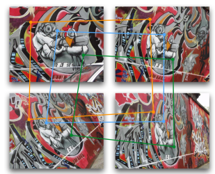
Figure 1: Illustration of consistent data association.

Our contributions are the following. 1) We propose a novel consensus-like algorithm for distributed data association. 2) We propose a decentralized version of the centralized state-of-art spectral method [pachauri2013solving]. 3) We show that both methods provably converge, do not depend on initialization, are parameter-free and guarantee global consistency. 4) We demonstrate the validity of proposed methods through both theoretical analysis and experimentation with synthetic and real data.

The rest of this paper is organized as follows. Section II includes a brief review of prior works. Section III introduces the reader to notation and preliminaries essential to understanding the main results of this paper. A rigorous problem formulation is the topic of Section IV. The two proposed methods are presented in Sections V and LABEL:sec:spectral respectively. Finally, experimental evaluation is presented in Section LABEL:sec:experiments.

II RELATED WORK

The cycle consistency has been explored in a variety of computer vision applications. For example, Zach et al. [zach2010disambiguating] studied the problem of multi-view reconstruction and proposed to identify unreliable geometric relations (e.g. relative poses) between views by measuring the consistencies along a number of cycles. Nguyen et al. [nguyen2011optimization] addressed the problem of finding point-wise maps among a collection of shapes and proposed to use the cycle consistency to identify the correctness of maps and replace the incorrect maps with the compositions of correct ones. Yan et al. [yan2015consistency, yan2016multi] considered the multiple graph matching problem and imposed the cycle consistency by penalizing the inconsistency during the optimization. Zhou et al. [zhou2015flowweb] developed a discrete searching algorithm that maximizes the cycle consistency to improve the dense optical flow in an image collection. Instead of iteratively optimizing the pairwise matches, [kim2012exploring, huang2012optimization, pachauri2013solving] showed that finding globally consistent associations from noisy pairwise associations can be formulated as a quadratic integer program and relaxed into a generalized Rayleigh problem and solved by the eigenvalue decomposition. More recently, Huang and Guibas [huang2013consistent] and Chen et al. [chen2014near] theoretically proved that the consistent associations could be exactly recovered from noisy measurements under certain conditions by convex relaxation and solved the problem by semidefinite programming. Zhou et al. [zhou2015multi] proposed to solve the problem by rank minimization and developed a more efficient algorithm. All of these works addressed problem in a centralized setting, i.e., all pairwise measurements are available and optimized jointly.

In the robotics community, numerous approaches for associating elements of two sets have been proposed and extensively used in single robot Simultaneous Localization And Mapping (SLAM) settings. These include but are not limited to Nearest Neighbor (NN) and Maximum Likelihood (ML) approaches [kaess2009covariance, zhou2006multi], Iterative Closest Point (ICP) [besl1992method], RANSAC [fischler1981random], Joint Compatibility Branch and Bound (JCBB) [neira2001data], Maximum Common Subgraph (MCS) [bailey2001localisation], Random Finite Sets (RFS) [vo2005sequential]. More recently, multi-robot localization and mapping algorithms have been developed. In almost all of them, the data association is addressed either in a pairwise fashion by directly generalizing data association techniques from the single robot case [cunningham2012fully, williams2002towards, fox2006distributed] or by considering all associations jointly in a centralized manner [indelman2014multi]. Closer to our approach is the work by Aragues et al. [aragues2011consistent] which is a decentralized method for finding inconsistencies based on cycle detection. However, the proposed inconsistency resolution algorithm comes without any optimality or guarantees.

III PRELIMINARIES, NOTATION AND DEFINITIONS

III-A Graph Theory

In this subsection, we review some elementary facts from graph theory. For an in depth analysis, we refer the reader to standard texts [godsil2013algebraic, mesbahi2010graph]. An undirected graph or simply a graph is denoted by the pair $\mathcal{G}=(\mathcal{V},\mathcal{E})$, where $\mathcal{V}=\{1,2,\ldots,n\}$ is the set of vertices and $\mathcal{E}\subseteq[\mathcal{V}]^{2}$ is the set of edges, where $[\mathcal{V}]^{2}$ denotes the set of unordered pairs of elements of $\mathcal{V}$. The neighborhood $\mathcal{N}_{i}$ of the vertex $i$ is the subset of $\mathcal{V}$ defined by $\mathcal{N}_{i}=\{j\in\mathcal{V}\ |\ {\{i,j\}\in\mathcal{E}}\}$. A path is a sequence ${i_{0}},{i_{1}},\ldots,{i_{m}}$ of distinct vertices such that $\{{i_{k-1}},{i_{k}}\}\in\mathcal{E}$ for all $k=1,\ldots,m$. A graph is connected if there is a path between any two vertices. Given a graph $\mathcal{G}=(\mathcal{V},\mathcal{E})$, its adjacency matrix is defined by

$$[A(\mathcal{G})]_{ij}=\left\{\begin{array}[]{ll}1,&\text{if }{\{i,j\}\in\mathcal{E}}\\ 0,&\text{otherwise }\end{array}\right.$$ (1)

The degree matrix $\Delta(\mathcal{G})$ is the diagonal matrix such that $[\Delta(\mathcal{G})]_{ii}=\left|\mathcal{N}_{i}\right|$, where $\left|\cdot\right|$ denotes the cardinality of a set.

A directed graph or digraph is denoted by the pair $\mathcal{G}=(\mathcal{V},\mathcal{E})$, where $\mathcal{E}\subseteq\mathcal{V}\times\mathcal{V}$. A weighted digraph $\mathcal{G}=(\mathcal{V},\mathcal{E},w)$ is a graph along with a function $w:\mathcal{E}\rightarrow\mathbb{R}_{+}$. The adjacency matrix of a weighted digraph is defined by

$$[A(\mathcal{G})]_{ij}=\left\{\begin{array}[]{ll}w(j,i),&\text{if }{(j,i)\in\mathcal{E}}\\ 0,&\text{otherwise }\end{array}\right.$$ (2)

Intuitively, if $[A(\mathcal{G})]_{ij}>0$ there is information flow from vertex $j$ to vertex $i$. The neighborhood $\mathcal{N}_{i}$ of the vertex $i$ is the subset of $\mathcal{V}$ defined by $\mathcal{N}_{i}=\{j\in\mathcal{V}\ |\ {(j,i)\in\mathcal{E}}\}$. The degree matrix $\Delta(\mathcal{G})$

$$[\Delta(\mathcal{G})]_{ii}=d_{\textrm{in}}(i)\doteq\sum_{j\in\mathcal{N}_{i}}[A(\mathcal{G})]_{ij}$$ (3)

A directed path is a sequence ${i_{0}},{i_{1}},\ldots,{i_{m}}$ of distinct vertices such that $({i_{k-1}},{i_{k}})\in\mathcal{E}$ for all $k=1,\ldots,m$. A digraph is strongly connected if there is a directed path between any two vertices. A digraph is a rooted out-branching tree if it has a vertex to which all other vertices are path connected and does not contain any cycles. A digraph is balanced if the in-degree $d_{in}(i)$ and the out-degree $d_{\textrm{out}}(i)\doteq\sum_{(i,j)\in\mathcal{E}}[A(\mathcal{G})]_{ji}$ are equal for all $i\in\mathcal{V}$. From this point and on, all graphs under consideration are assumed to be directed unless stated otherwise. The graph Laplacian $L(\mathcal{G})$ is defined as

$$L(\mathcal{G})=\Delta(\mathcal{G})-A(\mathcal{G})$$ (4)

By construction, $L(\mathcal{G})\mathbf{1}=0$. A digraph on $n$ vertices contains a rooted-out branching if and only the rank of its Laplacian is $n-1$. A matrix closely related to the graph Laplacian is defined by

$$F(\mathcal{G})\doteq(I+\Delta(\mathcal{G}))^{-1}(I+A(\mathcal{G}))$$ (5)

III-B Stochastic Matrices and Permutations

Stochastic matrices and their properties have been well studied in the area of distributed dynamical systems [jadbabaie2003coordination, olfati2007consensus, bertsekas1989parallel] and in probability theory in the context of computing invariant distributions of Markov chains [asmussen2008applied, bertsekas1989parallel]. A nonnegative square matrix is stochastic if all its row sums are equal to 1. The spectral radius $\rho(A)$ of a stochastic matrix $A$ is equal to 1 and it is an eigenvalue of $A$ since $A\mathbf{1}=\mathbf{1}$. The existence and the form of the limit $\lim_{k\rightarrow\infty}A^{k}$ depends on the multiplicity of $1$ as an eigenvalue. A nonegative square matrix $A$ is irreducible if its associated graph [horn2012matrix] is strongly connected. An irreducible stochastic matrix is primitive if it has only one eigenvalue of maximum modulus.

A nonnegative square matrix is doubly stochastic matrix if both its row sums and column sums are equal to 1. A doubly stochastic matrix is a permutation matrix if its elements are either 0 or 1. The sets of stochastic matrices and doubly stochastic matrices are compact convex sets. This is a rather useful property since it implies closure under convex combinations. For more details, regarding the theory of stochastic matrices, we refer the reader to [horn2012matrix].

Let $[n]\doteq\{1,2,\ldots,n\}$ for some positive integer $n$. A mapping $\pi:[n]\rightarrow[n]$ is a permutation of $[n]$ if it is bijective. The set of all permutations of $[n]$ forms a group under composition, termed the symmetric group $\mathfrak{S}_{n}$. A permutation $\pi\in\mathfrak{S}_{n}$ is represented by a $n\times n$ permutation matrix $\Pi$ defined by

$$[\Pi]_{ij}=\left\{\begin{array}[]{ll}1,&\text{if }\pi(j)=i\\ 0,&\text{otherwise }\end{array}\right.$$ (6)

or equivalently $\Pi e_{j}=e_{\pi(j)}$, where $e_{j}$ is the $j$th canonical basis vector. The simplest choice for a distance on $\mathfrak{S}_{n}$ is given by

$$d(\pi_{1},\pi_{2})=d(e,\pi_{1}^{-1}\pi_{2})\doteq n-\langle\Pi_{1},\Pi_{2}\rangle$$ (7)

where $\langle A,B\rangle\doteq\operatorname*{tr}(A^{T}B)$, $e$ is the identity map and $\Pi_{1},\Pi_{2}$ are the matrix representations of the permutations $\pi_{1}$ and $\pi_{2}$ respectively. The distance function defined above is simply the number of labels assigned differently by permutations $\pi_{1}$ and $\pi_{2}$. With a slight abuse of notation, we write $\Pi\in\mathfrak{S}_{n}$ meaning that $\Pi$ is an $n\times n$ permutation matrix.

III-C Consensus Algorithms

Consensus algorithms have been extensively studied in the control community [bertsekas1989parallel, jadbabaie2003coordination, olfati2007consensus]. In its simplest form, a consensus algorithm is a decentralized protocol in which the agents, modeled as vertices of a graph, try to reach agreement by communicating only with their neighbors. More formally, let $x_{i}(t)\in\mathbb{R}$ denote the state of agent $i$ at time time $t$. The, the simplest consensus protocol is given by

$$x_{i}(t+1)=\sum_{j\in\mathcal{N}_{i}\cup{i}}a_{ij}x_{j}(t)$$ (8)

where $a_{ij}\geq 0$ and $\sum_{j}a_{ij}=1$. A popular consensus protocol [olfati2007consensus], which converges to the average of the initial values provided that $\mathcal{G}$ is balanced, is described by

$$\mathbf{x}(t+1)=(I-\epsilon L(\mathcal{G}))\mathbf{x}(t)$$ (9)

where $\mathbf{x}=[x_{1},\ldots,x_{n}]^{T}$ and $0<\epsilon<1/\max_{i}[\Delta(\mathcal{G})]_{ii}$.

IV PROBLEM FORMALIZATION

In this section, we formalize the problem of consistent data association. We assume there are $n$ sensors observing $m$ targets. For instance, assume we have a set of $n$ cameras observing a scene in the world described by a set of $m$ feature points. Sensors communicate only with a subset of all sensors. Communication constraints between sensors are encoded by the sensor graph. The sensor graph is the digraph $G=(\mathcal{V},\mathcal{E})$ where $\mathcal{V}=\{1,2,\ldots,n\}$ and $(i,j)\in\mathcal{E}$ if there is information flow from sensor $i$ to $j$. The pairwise association $\pi_{ij}\in\mathfrak{S}_{m}$ is defined as follows: we have that $\pi_{ij}(l)=k$ if the $l$th target in $j$th sensor corresponds to the $k$th target in $i$th sensor. Observe that the pairwise associations $\pi_{ij}$ can be written as $\pi_{ij}=\pi_{i}\circ\pi_{j}^{-1}$, where $\pi_{i}\in\mathfrak{S}_{m}$ is the mapping from the labels of sensor $i$ to some global labels, termed the “universe of features” in some works [chen2014near, zhou2015multi]. This is analogous to the absolute position in Euclidean spaces in localization problems. We denote by $\widetilde{\pi}_{ij}\in\mathfrak{S}_{m}$ the, possibly erroneous, estimated pairwise association between sensor $i$ and $j$ and by $\widetilde{\Pi}_{ij}$ the corresponding matrix representation. Moreover, let $\Pi_{i}\doteq\rho(\pi_{i})$.

Related to the sensor graph is the data association graph $\mathcal{D}=(\mathcal{V}_{\mathcal{D}},{\mathcal{E}}_{\mathcal{D}},w_{\mathcal{D}})$, where $\mathcal{V}_{\mathcal{D}}=\mathcal{V}\times\{1,2,\ldots,m\}$. There is an edge from $(i,k)$ to $(j,l)$ if and only if $(i,j)\in\mathcal{E}$ and $[\widetilde{\Pi}_{ij}]_{kl}>0$. The corresponding edge weight is simply equal to $[\widetilde{\Pi}_{ij}]_{kl}$.

First, we need a precise definition of consistency.

Definition IV.1 (Consistency)

A set of pairwise associations $\{\widetilde{\pi}_{ij}\}_{(i,j)\in\mathcal{E}}$ is consistent if

$$\widetilde{\pi}_{ij}\circ\widetilde{\pi}_{jk}=\widetilde{\pi}_{ik}$$ (10)

for all valid indices $i,j,k$. A set of labels $\{\pi_{i}\}_{i=1}^{n}$ is consistent with respect to some consistent pairwise associations $\{\widetilde{\pi}_{ij}\}_{(i,j)\in\mathcal{E}}$, if

$$\widetilde{\pi}_{ij}=\pi_{i}\circ\pi_{j}^{-1},\qquad\forall(i,j)\in\mathcal{E}$$ (11)

Based on the definition of consistency, the problem of consistent data association is naturally defined as follows.

Definition IV.2 (Consistent data association)

Given pairwise associations $\{\widetilde{\pi}_{ij}\}_{(i,j)\in\mathcal{E}}$, find labels $\pi_{1},\ldots,\pi_{n}\in\mathfrak{S}_{m}$, such that

$$\widetilde{\pi}_{ij}=\pi_{i}\circ\pi_{j}^{-1},\qquad\forall\ (i,j)\in\mathcal{E}$$ (12)

Remark 1

Under the presence of noise, it might not be possible to find labels $\{\pi_{i}\}_{i=1}^{n}$ satisfying (12) exactly. Therefore, in practice we are looking for labels $\{\pi_{i}\}_{i=1}^{n}$ satisfying (12) as much as possible according to some criterion.

Figure 2: Example with $n=3$ sensors $S_{1},S_{2},S_{3}$ observing $m=3$ targets. Top: consistent data association. Bottom: inconsistent data association since $\pi_{12}\circ\pi_{23}(2)=3$ but $\pi_{31}(2)=2$.

V DISTRIBUTED AVERAGING

In the classic consensus algorithms, each agent updates his estimate of a collective quantity by taking convex combinations of the estimates of his neighbors. The problem at hand is different: we do not want all $\pi_{i}$’s to converge to the same value, rather to converge to a value satisfying consistency. The first obstacle one encounters is the combinatorial nature of the problem at hand. Therefore, we relax the domain of problem and work with doubly stochastic matrices instead of permutation matrices. This is a natural choice since the convex hull of the set of $m\times m$ permutation matrices is exactly the set of $m\times m$ doubly stochastic matrices.

V-A Algorithm

Based on the previous discussion, we propose the following update rule:

$$\Pi_{i}(t+1)=\dfrac{1}{\left|\mathcal{N}_{i}\right|+1}\bigl{(}\Pi_{i}(t)+\sum_{j\in\mathcal{N}_{i}}\widetilde{\Pi}_{ij}\Pi_{j}(t)\bigr{)}$$ (13)

Let $\mathbf{\Pi}=[\Pi_{1}^{T},\ldots,\Pi_{n}^{T}]^{T}$. The update rule (13) can be collectively written as

$$\mathbf{\Pi}(t+1)=F(\mathcal{D})\mathbf{\Pi}(t)$$ (14)

where $\mathcal{D}$ is the data association graph and $F(\mathcal{D})$ is defined in (5). The convergence properties of the update rule (13) depend solely on $\lim_{k\rightarrow\infty}F(\mathcal{D})^{k}$ and $\mathbf{\Pi}(0)$. These properties will be presented in Section LABEL:sec:properties.

After the convergence of Protocol (13), we discretize the solution by solving the assignment problem, formally defined by

$$\underset{\Pi_{i}}{\text{maximize}} \langle\widetilde{\Pi}_{i},\Pi_{i}\rangle$$ (15)

subject to $$\Pi_{i}\in\mathfrak{S}_{m}$$

where $\widetilde{\Pi}_{i}$ is the result of Protocol (13). The assignment problem can be solved using the Hungarian algorithm [kuhn1955hungarian] in $O(m^{3})$ time.