Parallel transport along Seifert manifolds and fractional monodromy

Abstract.

The notion of fractional monodromy was introduced by Nekhoroshev, Sadovskií and Zhilinskií as a generalization of standard (‘integer’) monodromy in the sense of Duistermaat from torus bundles to singular torus fibrations. In the present paper we prove a general result that allows to compute fractional monodromy in various integrable Hamiltonian systems. In particular, we show that the non-triviality of fractional monodromy in $2$ degrees of freedom systems with a Hamiltonian circle action is related only to the fixed points of the circle action. Our approach is based on the study of a specific notion of parallel transport along Seifert manifolds.

1. Introduction

A fundamental notion in classical mechanics is the notion of Liouville integrability. A Hamiltonian system

$$\dot{x}=X_{H},\ \ \omega(X_{H},\cdot)=-dH,$$

on the $2n$-dimensional symplectic manifold $(M,\omega)$ is called Liouville integrable if there exist almost everywhere independent functions $F_{1}=H,\ldots,F_{n}$ such that all Poisson brackets vanish:

$$\{F_{i},F_{j}\}=\omega(X_{F_{i}},X_{F_{j}})=0.$$

Various Hamiltonian systems, such as the Kepler and two-centers problem, the problem of $n\leq 3$ point vortices, Euler, Lagrange and Kovalevskaya tops, are integrable in this sense.

The topological significance of Liouville integrability reveals itself in the Arnol’d-Liouville theorem [1]. Assume that the integral map

$$F=(F_{1},\ldots,F_{n})\colon M\to\mathbb{R}^{n}$$

is proper. The theorem states that a tubular neighborhood of a connected regular fiber $F^{-1}(\xi_{0})$ is a trivial torus bundle $D^{n}\times T^{n}$ admitting (semi-local) action-angle coordinates

$$I\in D^{n}\ \mbox{ and }\ \varphi\mod 2\pi\in T^{n},\ \ \omega=dI\wedge d\varphi.$$

In particular, $F$ is a singular torus fibration and on each torus $\{\xi\}\times T^{n}$ the motion is quasi-periodic.

The question whether and when the action-angle coordinates exist globally was answered in [26, 12]. It turns out [26] that global action-angle coordinates exist if the set $R\subset image(F)$ of regular values of $F$ is such that

$$\pi_{1}(R,\xi_{0})=0\ \mbox{ and}\ H^{2}(R,\mathbb{R})=0.$$

Obstructions that give necessary and sufficient conditions for the existence of global action-angle coordinates were given by Duistermaat; see [12, 24]. One such obstruction is called (standard) monodromy. It appears only if $\pi_{1}(R,\xi_{0})\neq 0$ and entails the non-existence of global action coordinates.

Since the work of Duistermaat, standard monodromy has been observed in many integrable systems of classical mechanics as well as in integrable approximations to molecular and atomic systems. In the typical case of $n=2$ degrees of freedom non-trivial monodromy is manifested by the presence of the so-called focus-focus points of the integral fibration $F$ [23, 25, 35]. Such a result is often referred to as geometric monodromy theorem. It has been recently observed in [17] that the geometric monodromy theorem is a consequence of the following topological result.

Theorem 1.1.

([7, §4.3.2], [17]) Assume that $n=2$ and that $F\colon F^{-1}(R)\to R$ is invariant under a free fiber-preserving $\mathbb{S}^{1}$ action. For a simple closed curve $\gamma\subset R$ set $E=F^{-1}(\gamma)$ and $B=E/\mathbb{S}^{1}$. Then the monodromy of the $2$-torus bundle $F\colon E\to\gamma$ is given by

$$\begin{pmatrix}1&\langle{\bf e},B\rangle\\ 0&1\end{pmatrix}\in\mathrm{SL}(2,\mathbb{Z}),$$

where ${\bf e}$ is the Euler class of the principal circle bundle $\rho\colon E\to B$.

Remark 1.2.

The number $\langle{\bf e},B\rangle$, which is obtained by integrating the Euler class over the base $B$, is called the Euler (or the Chern) number of the principal circle bundle $\rho\colon E\to B$. Theorem 1.1 tells us that this Euler number determines the monodromy of the $2$-torus bundle $F\colon E\to\gamma$ and vice versa.

In a neighborhood of the focus-focus fiber there exists a unique (up to orientation) system preserving $\mathbb{S}^{1}$ action that is free outside focus-focus points [35]. On a small $3$-sphere $S^{3}_{\varepsilon}$ around a focus-focus point it defines a circle bundle with the Euler number $\langle{\bf e},S^{3}_{\varepsilon}\rangle=1$, the so-called anti-Hopf fibration. It follows from Stokes’ theorem that for a small loop $\gamma$ around the focus-focus critical value the Euler number $\langle{\bf e},B\rangle$ equals the number of focus-focus points on the singular fiber. In particular, standard monodromy along $\gamma$ is non-trivial. More details can be found in [17]; see also Section 2.

Even though standard monodromy is related to singularities of the torus fibration $F$, it is an invariant of the regular, non-singular part $F\colon F^{-1}(R)\to R$. An invariant that generalizes standard monodromy to singular torus fibrations is called fractional monodromy [28]. We note that fractional monodromy is not a complete invariant of such fibrations — it contains less information than the marked molecule in Fomenko-Zieschang theory [19, 7, 6] — but it is important for applications and appears, for instance, in the so-called $m$:$(-n)$ resonant systems [28, 27, 31, 30, 15]; see Section 4.1 for details.

It was observed by Bolsinov et al. [6] that in $m$:$(-n)$ resonant systems the circle action defines a Seifert fibration on a small $3$-sphere around the equilibrium point and that the Euler number of this fibration equals the number appearing in the matrix of fractional monodromy, cf. Remark 1.2. The question that remained unresolved is why this equality holds. In the present paper we give a complete answer to this question by proving the following results.

(i) Parallel transport and, therefore, fractional monodromy can be naturally defined for closed Seifert manifolds (with an orientable base of genus $g>0$).

(ii) The fractional monodromy matrix is given by the Euler number of the associated Seifert fibration. In the case of integrable systems, this Euler number can be computed in terms of the fixed points of the circle action.

The latter result generalizes the corresponding results of [15, 17] and, in particular, Theorem 1.1, thus demonstrating that for standard and fractional monodromy the circle action is more important than the precise form of the integral map $F$.

We note that the importance of Seifert fibrations in integrable systems was discovered by Fomenko and Zieschang. In their classification theorem [19, 7] Seifert manifolds play a central role: regular isoenergy surfaces of integrable nondegenerate systems with $2$ degrees of freedom admit decomposition into families, each of which has a natural structure of a Seifert fibration. In our case of a global circle action there is only one such family, which has a certain label associated to it, the so-called $n$-mark [7]. In fact, this $n$-mark coincides with the Euler number that appears in Theorem 1.1 and is related to the Euler number in the general case; see Remark 1.4. Our results therefore show how exactly this $n$-mark determines fractional monodromy.

1.1. $1$:$(-2)$ resonant system

Here, as a preparation to the more general setting of Sections 2 and 3, we discuss the famous example of a Hamiltonian system with fractional monodromy due to Nekhoroshev, Sadovskií and Zhilinskií [28].

Consider $\mathbb{R}^{4}$ with the standard symplectic structure $\omega=dq\wedge dp$. Define the energy by

$$H=2q_{1}p_{1}q_{2}+(q_{1}^{2}-p_{1}^{2})p_{2}+R^{2},$$

where $R=\frac{1}{2}(q_{1}^{2}+p_{1}^{2})+(q_{2}^{2}+p_{2}^{2})$, and the momentum by

$$J=\dfrac{1}{2}(q_{1}^{2}+p_{1}^{2})-(q_{2}^{2}+p_{2}^{2}).$$

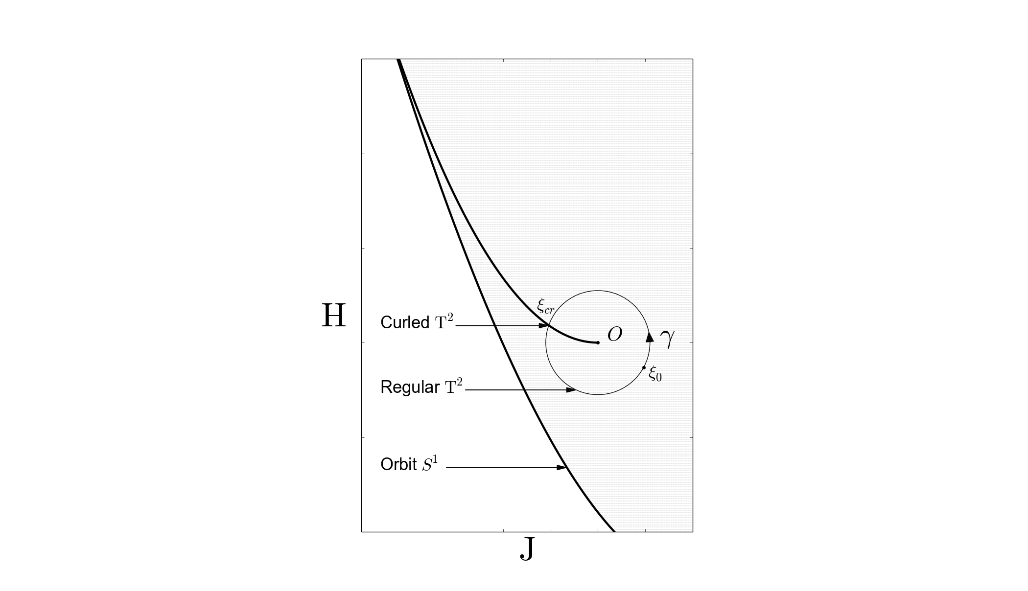
Figure 1. The bifurcation diagram of the $1$:$(-2)$ resonant system. Critical values are colored black; the set $R$ is shown gray; the closed curve $\gamma$ around the origin intersects the hyperbolic branch of critical values once and transversely.

A straightforward computation shows that the functions $H$ and $J$ Poisson commute, so the map $F=(J,H)$ defines an integrable Hamiltonian system on $\mathbb{R}^{4}$. The bifurcation diagram, that is, the set of critical values of $F$, is depicted in Figure 1. Let

$$R=\{\xi\in\textup{image}(F)\mid\xi\mbox{ is a regular value of }F\}.$$

Since the fundamental group of the set $R$ vanishes, there is no monodromy and, thus, the $2$-torus bundle $F\colon F^{-1}(R)\to R$ admits a free fiber-preserving action of a $2$-torus. We observe that the acting torus contains a subgroup $\mathbb{S}^{1}$ whose action extends from $F^{-1}(R)$ to the whole $\mathbb{R}^{4}$. Indeed, such an action is given by the Hamiltonian flow of $J$. In complex coordinates $z=p_{1}+iq_{1}$ and $w=p_{2}+iq_{2}$ it has the form

(1) $$(t,z,w)\mapsto(e^{it}z,e^{-2it}w),\ t\in\mathbb{S}^{1}.$$

From above it follows that the $\mathbb{S}^{1}$ action is free on $F^{-1}(R)$ and, moreover, has a trivial Euler class. However, on the whole phase space $\mathbb{R}^{4}$ the action is no longer trivial: the origin is fixed and the punctured plane

$$P=\{(q,p)\mid q_{1}=p_{1}=0\mbox{ and }q_{2}^{2}+p_{2}^{2}\neq 0\}$$

consists of points with $\mathbb{Z}_{2}$ isotropy group. This implies that the Euler number of the Seifert $3$-manifold $F^{-1}(\gamma)$, where $\gamma$ is as in Fig. 1, equals $1/2\neq 0$. Indeed, Stokes’ theorem implies that the Euler number of $F^{-1}(\gamma)$ coincides with the Euler number of a small $3$-sphere around the origin $z=w=0$. The latter Euler number equals $1/2$ because of (1).

The following result shows that the non-trivial Euler number of the Seifert manifold $F^{-1}(\gamma)$ enters the monodromy context, giving rise to what is now known as fractional monodromy.

Lemma 1.3.

Let $\mathbb{Z}_{2}=\{1,-1\}$ denote the order two subgroup of the acting circle $\mathbb{S}^{1}.$ The quotient space $F^{-1}(\gamma)/\mathbb{Z}_{2}$ is the total space of a torus bundle over $\gamma$. Its standard monodromy is given by $\begin{pmatrix}1&1\\ 0&1\end{pmatrix}\in\mathrm{SL}(2,\mathbb{Z}).$

Proof.

Let $\xi\in\gamma\cap R$. Then the fiber $F^{-1}(\xi)$ is a $2$-torus. Since the $\mathbb{S}^{1}$ action is free on this fiber, the quotient $F^{-1}(\xi)/\mathbb{Z}_{2}$ is a $2$-torus as well.

Consider the critical value $\xi_{cr}\in\gamma.$ Its preimage $F^{-1}(\xi_{cr})$ is the so-called curled torus; see Fig. 2(b).

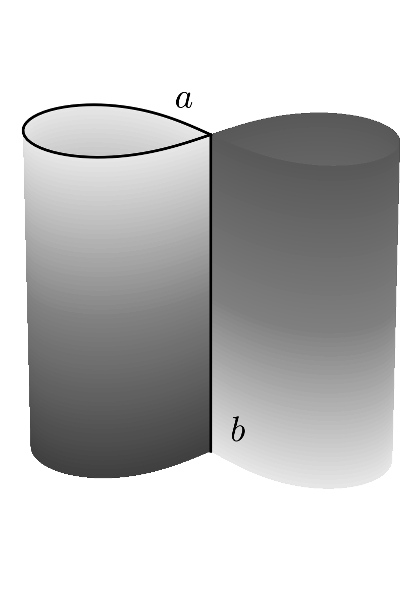
(a) Cycles $(a,b)$

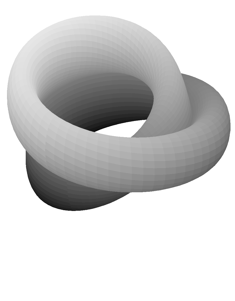
(b) Curled torus

Figure 2. Representation of a curled torus. Take a cylinder over the figure ‘eight’, as shown in Figure $(a)$. Glue the upper and lower halves of this cylinder after rotating the upper part by $\pi$. The resulting surface is a curled torus $(b)$.

In this case there is a ‘short’ orbit $b$ of the $\mathbb{S}^{1}$ action, formed by the fixed points of the $\mathbb{Z}_{2}$ action. The ‘short’ orbit passes through the tip of the cycle $a$; see Fig. 2(a). Other orbits are ‘long’, that is, principal. From this description it follows that after taking the $\mathbb{Z}_{2}$ quotient only half of the cylinder survives and, thus, $F^{-1}(\xi_{cr})/\mathbb{Z}_{2}$ is topologically a $2$-torus. In view of [19], we have shown that

$$F\colon F^{-1}(\xi)/\mathbb{Z}_{2}\to\gamma$$

is a torus bundle. In order to complete the proof of the theorem it is left to apply Theorem 1.1. Indeed, since the Euler number of $F^{-1}(\gamma)$ equals $1/2$, the Euler number of $F^{-1}(\gamma)/\mathbb{Z}_{2}$ equals $1$. ∎

Remark 1.4.

Lemma 1.3 can be reformulated by saying that the $n$-mark of the loop molecule associated to $\gamma$ equals $1$. The molecule has the form shown in Fig. 3. Note that the $A^{*}$ atom corresponds to the curled torus Fig. 2(b). A similar statement holds for higher-order resonances.

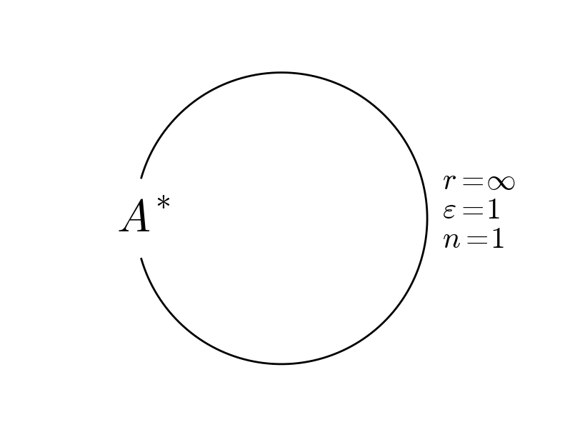
Figure 3. The loop molecule associated to $\gamma$.

Remark 1.5.

We note that the symplectic structure on an open neighborhood $O$ of the manifold $F^{-1}(\gamma)$ does not descend to the $\mathbb{Z}_{2}$-quotient. Hence, the fibration $F\colon O/\mathbb{Z}_{2}\to\mathbb{R}^{2}$ does not carry a natural Lagrangian structure and Duistermaat’s monodromy (parallel transport) along $\gamma$ is not defined. Instead, we use the more general Definition 1.6.

Cutting the manifold $F^{-1}(\gamma)/\mathbb{Z}_{2}$ along any fiber $F^{-1}(\xi_{0})/\mathbb{Z}_{2},\,\xi_{0}\in\gamma\cap R,$ we get a manifold $X$ with the boundary $\partial X=X_{0}\sqcup X_{1}$ consisting of the two tori $X_{i}.$ Following [15], we define the parallel transport using the connecting homomorphism of the long exact sequence of the pair $(X,\partial X)$.

Definition 1.6.

The cycle $\alpha_{1}\in H_{1}(X_{1})$ is a parallel transport of the cycle $\alpha_{0}\in H_{1}(X_{0})$ along $X$ if

$$(\alpha_{0},-\alpha_{1})\in\partial_{*}(H_{2}(X,\partial X)),$$

where $\partial_{*}$ is the connecting homomorphism of the exact sequence

$$\cdots\rightarrow H_{2}\left(X\right)\rightarrow H_{2}\left(X,\partial X\right)\xrightarrow{\\ \partial_{*}\\ }H_{1}\left(\partial X\right)\rightarrow H_{1}\left(X\right)\rightarrow\cdots$$

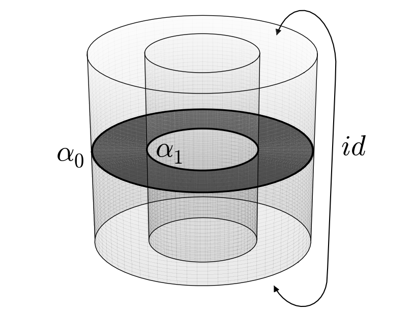
Figure 4. Parallel transport along $X$.

Remark 1.7.

Definition 1.6 is applicable to an arbitrary manifold $X$ with boundary $\partial X=X_{0}\sqcup X_{1}$. For compact $3$ manifolds it may be reformulated as follows (see [21]): $\alpha_{1}$ is a parallel transport of $\alpha_{0}$ along $X$ if there exists an oriented $2$-dimensional submanifold $S\subset X$ that ‘connects’ $\alpha_{0}$ and $\alpha_{1}$:

$$\partial S=S_{0}\sqcup S_{1}\mbox{ and }[S_{i}]=(-1)^{i}\alpha_{i}\in H_{1}(X_{i});$$

see Fig. 4. We note, however, that even for compact $3$-manifolds it might happen that, for a given homology cycle, the parallel transport is not defined or is not unique. For manifolds $F^{-1}(\gamma)$ and $F^{-1}(\gamma)/\mathbb{Z}_{2}$ (and, more generally, for Seifert manifolds) the parallel transport is unique; see Theorem 2.5.

From Lemma 1.3 we infer that, in a homology basis of the fiber $F^{-1}(\xi_{0})/\mathbb{Z}_{2}$, the parallel transport has the form of the monodromy matrix

$$\begin{pmatrix}1&1\\ 0&1\end{pmatrix}\in\mathrm{SL}(2,\mathbb{Z}).$$

For the fibration $F^{-1}(\gamma)\to\gamma$ this manifests the presence of nontrivial fractional monodromy.

Theorem 1.8.

([28]) Let $(a_{0},b_{0})$ be an integer basis of $H_{1}(F^{-1}(\xi_{0}))$, where $b$ is given by any orbit of the $\mathbb{S}^{1}$ action. The parallel transport is unique and has the form $2a_{0}\mapsto 2a_{0}+b_{0}$ and $b_{0}\mapsto b_{0}$.

Remark 1.9.

When written formally in an integer basis $(a_{0},b_{0})$, parallel transport has the form of a rational matrix

$$\begin{pmatrix}1&1/2\\ 0&1\end{pmatrix}\in\mathrm{SL}(2,\mathbb{Q}),$$

called the matrix of fractional monodromy.

Since the pioneering work [28], various proofs of Theorem 1.8 appeared; see [16, 31, 8, 32] and [15]. Our proof, which is based on the singularities of the circle action, shows that

• the fixed point $\boldsymbol{0}\in\mathbb{R}^{4}$ of the $\mathbb{S}^{1}$ action and

• the short orbit $b$ with $\mathbb{Z}_{2}$ isotropy

manifest the presence of fractional monodromy in this $1{:}(-2)$ resonant system. A similar kind of result holds in a general setting of Seifert manifolds; see Section 2, and, in particular, in the setting of Hamiltonian systems with $m{:}(-n)$ resonance; see Subsection 4.1.

1.2. The paper is organized as follows

In Section 2 we consider a general setting of Seifert fibrations. We show that the parallel transport along the total space of such a fibration is given by its Euler number and the orders of the exceptional orbits; see Theorems 2.5. In the case when a Seifert fibration admits an equivariant filling, the Euler number is given by the fixed points of the circle action inside the filling manifold; see Theorem 2.8.

In Section 3.2, after discussing the concepts of standard and (more general) fractional monodromy in integrable Hamiltonian systems, we apply the results of Section 2 to fractional monodromy in the $2$ degrees of freedom case; see Theorems 3.9 and 3.12. These theorems specify the subgroup of homology cycles that admit parallel transport, and give a formula for the computation of the fractional monodromy. These results, moreover, demonstrate that for standard and fractional monodromy the circle action is more important than the precise form of the integral map.

Examples are investigated in Section 4. The proof of Theorem 2.5 is given in Section 5. We conclude with a discussion in Section 6.

2. Parallel transport along Seifert manifolds

2.1. Seifert fibrations

In the present subsection we recall the notions of a Seifert fibration and its Euler number. For a more detailed exposition we refer to [18].

Definition 2.1.

Let $X$ be a compact orientable $3$-manifold (closed or with boundary) which is invariant under an effective fixed point free $\mathbb{S}^{1}$ action. Assume that the $\mathbb{S}^{1}$ action is free on the boundary $\partial X$. Then

$$\rho\colon X\to B=X/\mathbb{S}^{1}$$

is called a Seifert fibration. The manifold $X$ is called a Seifert manifold.

Remark 2.2.

From the slice theorem [2, Theorem I.2.1] (see also [5]) it follows that the quotient $B=X/\mathbb{S}^{1}$ is an orientable topological $2$-manifold. Seifert fibrations are also defined in a more general setting when the base $B$ is non-orientable; see [18], [22]. However, in this case there is no $\mathbb{S}^{1}$ action and the parallel transport is not unique; see Remark 2.7. We will therefore consider the orientable case only.

Consider a Seifert fibration

$$\rho\colon X\to B=X/\mathbb{S}^{1}$$

of a closed Seifert manifold $X$. Let $N$ be the least common multiple of the orders of the exceptional orbits, that is, the orders of non-trivial isotropy groups. Since $X$ is compact, the number $N$ is well defined. Denote by $\mathbb{Z}_{N}$ the order $N$ subgroup of the acting circle $\mathbb{S}^{1}$. The subgroup $\mathbb{Z}_{N}$ acts on the Seifert manifold $X$. We thus have the reduction map $h\colon X\to X^{\prime}=X/\mathbb{Z}_{N}$ and the commutative diagram

with $\rho^{\prime}$ defined via $\rho=\rho^{\prime}\circ h$. By the construction, $\rho^{\prime}\colon X^{\prime}\to B$ is a principal circle bundle over $B$. We denote its Euler number by $e(X^{\prime})$.

Definition 2.3.

The Euler number of the Seifert fibration $\rho\colon X\to B=X/\mathbb{S}^{1}$ is defined by $e(X)=e(X^{\prime})/N.$

Remark 2.4.

We note that a closed Seifert manifold $X$ can have non-isomorphic $\mathbb{S}^{1}$ actions with different Euler numbers. Indeed, let $m$ and $n$ be co-prime integers. Consider the $\mathbb{S}^{1}$ action

$$(t,z,w)\mapsto(e^{imt}z,e^{-int}w),\ t\in\mathbb{S}^{1},$$

on the $3$-sphere $S^{3}=\{(z,w)\mid|z|^{2}+|w|^{2}=1\}$. Then the Euler number of the fibration $\rho\colon S^{3}\to S^{3}/\mathbb{S}^{1}$ equals $1/mn$. Despite this non-uniqueness, we sometimes refer to $e(X)$ as the Euler number of the Seifert manifold $X$. This should not be a cause of confusion since it will be always clear from the context what is the underlying $\mathbb{S}^{1}$ action.

In the following Subsection 2.2 we show that the Euler number of a Seifert fibration is an obstruction to the existence of a trivial parallel transport; see Definition 1.6.

2.2. Parallel transport

Consider a Seifert fibration $\rho\colon X\to B=X/\mathbb{S}^{1}$ such that the boundary $\partial X=X_{0}\sqcup X_{1}$ consists of two $2$-tori $X_{0}$ and $X_{1}$. Take an orientation and fiber preserving homeomorphism $f\colon X_{0}\to X_{1}$. Any homology basis $(a_{0},b_{0})$ of $H_{1}(X_{0})$ can be then mapped to the homology basis

$$(a_{1}=f_{\star}(a_{0}),b_{1}=f_{\star}(b_{0}))$$

of $H_{1}(X_{1}).$ In what follows we assume that $b_{0}$ is equal to the homology class of a (any) fiber of the Seifert fibration on $X_{0}.$ Let

$$X(f)=X/\sim,\ \ X_{0}\ni x_{0}\sim f(x_{0})\in X_{1},$$

be the closed Seifert manifold that is obtained from $X$ by gluing the boundary components using $f$.

Finally, let $N$ be the least common multiple of $n_{j}$ – the orders of the exceptional orbits. With this notation we have the following result.

Theorem 2.5.

The parallel transport along $X$ is unique. Only linear combinations of $Na_{0}$ and $b_{0}$ can be parallel transported along $X$ and under the parallel transport

$$\begin{split}Na_{0}&\mapsto Na_{1}+kb_{1}\\ b_{0}&\mapsto b_{1}\end{split}$$

for some integer $k=k(f)$ which depends only on the isotopy class of $f.$ Moreover, the Euler number of $X(f)$ is given by $e(f)=k(f)/N.$

Proof.

See Section 5. ∎

Remark 2.6.

We note that (by the construction) $X(f)/\mathbb{S}^{1}$ has genus $g>0$ and hence is not a sphere. It follows that the $\mathbb{S}^{1}$ action on $X$ and $X(f)$ is unique up to isomorphism; see [21, Theorem 2.3].

Remark 2.7.

Even if the base $B$ is non-orientable, the group $\partial_{*}(X,\partial X)$ is still isomorphic to $\mathbb{Z}^{2}$. However, in this case, $\partial_{*}(X,\partial X)$ is spanned by $(b_{0},b_{1})$ and $(2b_{0},0)$. It follows that no multiple of $a_{0}$ can be parallel transported along $X$ and that the parallel transport is not unique.

2.3. The case of equivariant filling

Theorem 2.5 shows that the Euler number of a Seifert manifold can be computed in terms of the parallel transport along this manifold. But conversely, if we know the Euler number and the orders of exceptional orbits of a Seifert manifold, we also know how the parallel transport acts on homology cycles. In applications the orders of exceptional orbits are often known. In order to compute the Euler number one may then use the following result.

Theorem 2.8.

Let $M$ be a compact oriented $4$-manifold that admits an effective circle action. Assume that the action is fixed-point free on the boundary $\partial M$ and has only finitely many fixed points $p_{1},\ldots,p_{\ell}$ in the interior. Then

$$e(\partial M)=\sum\limits_{k=1}^{\ell}\dfrac{1}{m_{k}n_{k}},$$

where $(m_{k},n_{k})$ are isotropy weights of the fixed points $p_{k}$.

Remark 2.9.

Recall that near each fixed point $p_{k}$ the $\mathbb{S}^{1}$ action can be linearized as

(2) $$(t,z,w)\mapsto(e^{im_{k}t}z,e^{-in_{k}t}w),\ t\in\mathbb{S}^{1},$$

in appropriate coordinates $(z,w)$ that are positive with respect to the orientation of $M$. The isotropy weights $m_{k}$ and $n_{k}$ are co-prime integers. In particular, none of them is equal to zero.

Remark 2.10.

In the above theorem neither $M$ nor $\partial M$ are assumed to be connected. The orientation on $\partial M$ is induced by $M$.

Proof of Theorem 2.8. Eq. (2) implies that for each fixed point $p_{k}$ there exists a small closed $4$-ball $B_{k}\ni p_{k}$ invariant under the action. Denote by $Z$ the manifold $Z=M\setminus\bigcup_{k=1}^{\ell}B_{k}.$ Let $N$ be a common multiple of the orders of all exceptional orbits in $M$ and $\mathbb{Z}_{N}$ be the order $N$ subgroup of the acting circle $\mathbb{S}^{1}$. Set

$$X=Z/\mathbb{Z}_{N}\ \ \ \mbox{ and }\ \ \ Y=Z/\mathbb{S}^{1}.$$

Denote by $\Pr\colon X\to Y$ the natural projection that identifies the orbits of the $\mathbb{S}^{1}/\mathbb{Z}_{N}$ action. By the construction the triple $(X,Y,\Pr)$ is a principal circle bundle.

Because of the slice theorem [2] the spaces $X$ and $Y$ are topological manifolds (with boundaries). The boundary $\partial Y$ is a disjoint union of the closed $2$-manifold $B=\partial M/\mathbb{S}^{1}$ and the $2$-spheres $S^{2}_{k}=\partial B_{k}/\mathbb{S}^{1}.$ Let $i_{B}\colon B\to Y$ and $i_{k}\colon S^{2}_{k}\to Y$ be the corresponding inclusions.

Denote by ${\bf e}_{Y}\in H^{2}(Y)$ the Euler class of the circle bundle $(X,Y,\Pr)$. By the functoriality $i^{*}_{B}({\bf e}_{Y})$ and $i^{*}_{k}({\bf e}_{Y})$ are the Euler classes of the circle bundles $(\Pr^{-1}(B),B,\Pr)$ and $(\Pr^{-1}(S^{2}_{k}),S^{2}_{k},\Pr)$, respectively. Hence

$$\langle{\bf e}_{Y},i_{B}(B)\rangle=\langle i^{*}_{B}({\bf e}_{Y}),B\rangle=Ne(\partial M)$$

and analogously

$$\langle{\bf e}_{Y},i_{k}(S^{2}_{k})\rangle=\langle i^{*}_{k}{\bf e}_{Y},S^{2}_{k}\rangle=\dfrac{N}{m_{k}n_{k}}.$$

The equality

$$\langle{\bf e}_{Y},i_{B}(B)-\sum_{k=1}^{\ell}i_{k}(S^{2}_{k})\rangle=\langle{\bf e}_{Y},\partial Y\rangle=0$$

completes the proof. ∎

3. Monodromy in integrable systems

3.1. Historical and mathematical background

Standard monodromy was introduced by Duistermaat in [12] as an obstruction to the existence of global action coordinates in integrable Hamiltonian systems. Since the early work [12], non-trivial monodromy has been observed in the (quadratic) spherical pendulum ([4, 14]) [12, 9], the Lagrange top [10], the Hamiltonian Hopf bifurcation [13], the champagne bottle [3], the coupled angular momenta [29], the hydrogen atom in crossed fields [11], the two-centers problem [34, 33] and many other systems. A common aspect of most of these systems is the presence of focus-focus singular points of the Lagrangian fibration. It is known that the presence of such singular points is sufficient for the monodromy to be nontrivial in the general case (geometric monodromy theorem) [23, 25, 35].

The definition of standard monodromy in the sense of Duistermaat [12] reads as follows. Consider a Lagrangian $n$-torus bundle $F\colon M\to R$ over a $n$-dimensional manifold $R$. By definition, this means that $M$ is a symplectic manifold and that each fiber $F^{-1}(\xi)$ is a Lagrangian submanifold of $M$.

Remark 3.1.

In the context of integrable systems $R\subset\mathbb{R}^{n}$ and $F$ is given by $n$ Poisson commuting functions. Conversely, every chart $(V,\chi)$ of $R$ gives rise to an integrable system on $F^{-1}(V)\subset M$ with the integral map $F\circ\chi$.

There is a well-defined action of the fibers of $\Pr\colon T^{*}R\to R$ on the fibers of $F\colon M\to R$, which, in every chart $(V,\chi)$, is given by the flow of $n$ Poisson commuting functions $F\circ\chi$; see [12] and [24]. For each $\xi\in R$ the stabilizer of the $\mathbb{R}^{n}_{\xi}=\Pr^{-1}(\xi)$ action on $T^{n}_{\xi}=F^{-1}(\xi)$ is a lattice $\mathbb{Z}^{n}_{\xi}\subset\mathbb{R}^{n}_{\xi}$. The union of these lattices covers the base manifold $R$:

$$\Pr\colon\bigcup\mathbb{Z}^{n}_{\xi}\to R.$$

Definition 3.2.

The (standard) monodromy of the Lagrangian $n$-torus bundle $F\colon M\to R$ is defined as the representation

$$\rho\colon\pi_{1}(R,\xi_{0})\to\textup{Aut}\,\mathbb{Z}^{n}_{\xi_{0}}\simeq\mathrm{GL}(n,\mathbb{Z})$$

of the fundamental group $\pi_{1}(R,\xi_{0})$ of the base $R$ in the group of automorphisms of $\mathbb{Z}^{n}_{\xi_{0}}$. For each element $[\gamma]\in\pi_{1}(R,\xi_{0})$, the automorphism $\rho([\gamma])$ is called the (standard) monodromy along $\gamma$

Remark 3.3.

We note that the lattices $\mathbb{Z}^{n}_{\xi}$ give a unique local identification of cotangent spaces of $T^{*}R$, that is, a flat connection. Thus, standard monodromy is given by the parallel transport (holonomy) of this connection.

The following lemma shows that, in the case of Lagrangian torus bundles, the parallel transport in the sense of Definition 1.6 coincides with the parallel transport of the flat connection, given in Remark 3.3.

Lemma 3.4.

Let $\gamma=\gamma(t)$ be a continuous curve and

(3) $$X=\{(x,t)\in M\times[0,1]\colon F(x)=\gamma(t)\}.$$

Then $(\alpha_{0},-\alpha_{1})\in\partial_{*}(H_{2}(X,\partial X))$ if and only if the cycle $\alpha_{1}$ is a parallel transport of $\alpha_{0}$ in the sense of Remark 3.3.

Proof. By homotopy invariance, we can assume that $\gamma$ is smooth. Let $(0=t_{0}\leq\ldots\leq t_{n}=1)$ be a sufficiently fine partition of the segment $[0,1]$. Then, for each $i$, we have

$$\gamma([t_{i},t_{i+1}])\subset V_{i},$$

where $V_{i}$ is a small open neighborhood $V_{i}\subset R$. By the Arnol’d-Liouville theorem [1], the two notions of parallel transport along $\gamma|_{[t_{i},t_{i+1}]}$ coincide. The result follows. ∎

Remark 3.5.

Let $\gamma$ be a simple curve. If $\gamma(0)\neq\gamma(1)$, then the manifold $X$ in (3) is homeomorphic to $F^{-1}(\gamma)$. If $\gamma(0)=\gamma(1)=\xi_{0}$, then the manifold $X$ is obtained from $F^{-1}(\gamma)$ by cutting along the fiber $F^{-1}(\xi_{0})$.

Fractional monodromy was introduced in [28] as a generalization of standard monodromy in the sense of Duistermaat from Lagrangian torus bundles to singular Lagrangian fibrations. Since the pioneering work [28], non-trivial fractional monodromy has been demonstrated in several integrable Hamiltonian systems [27, 20, 31, 15].

What has been missing until now for fractional monodromy is a result that associates fractional monodromy to certain singular points of the Lagrangian fibration in the same spirit as the geometric monodromy theorem associates standard monodromy to focus-focus singular points. In the next subsection 3.2 we give such a result for fractional monodromy in the case when the fibration is invariant under an effective circle action. Specifically, we show that fractional monodromy is completely determined by the singularities of the corresponding circle action and that, in certain cases, fractional monodromy can be computed in terms of the fixed points of this action, just as standard monodromy [17].

The definition of fractional monodromy (in the sense of [28] and [15]) reads as follows. Consider a singular Lagrangian fibration $F\colon M\to R$ over a $n$-dimensional manifold $R$, given by a proper integral map $F$. Locally, such a fibration gives an integrable Hamiltonian system. Let $\gamma=\gamma(t)$ be a continuous closed curve in $F(M)$ such that the space

$$X=\{(x,t)\in M\times[0,1]\colon F(x)=\gamma(t)\}$$

is connected and such that $\partial X=X_{0}\sqcup X_{1}$ is a disjoint union of two regular tori $X_{0}=F^{-1}(\gamma(0))$ and $X_{1}=F^{-1}(\gamma(1)).$ Set

$$H^{0}_{1}=\{\alpha_{0}\in H_{1}(X_{0})\mid\alpha_{0}\mbox{ can be parallel transported along }X\}.$$

Definition 3.6.

If the parallel transport along $X$ defines an automorphism of the group $H^{0}_{1}$, then this automorphism is called fractional monodromy along $\gamma$.

Remark 3.7.

As was mentioned in Subsection 1.1, in the singular case the notion of parallel transport in the sense of Remark 3.3 is not defined. Instead, the more general Definition 1.6 is used.

3.2. Applications to integrable systems

Consider a singular Lagrangian fibration $F\colon M\to R$ over a $2$-dimensional manifold $R$. Assume that the map $F$ is proper and invariant under an effective $\mathbb{S}^{1}$ action. Take a simple closed curve $\gamma=\gamma(t)$ in $F(M)$ that satisfies the following regularity conditions:

1. the fiber $F^{-1}(\gamma(0))$ is regular and connected;

2. the $\mathbb{S}^{1}$ action is fixed-point free on the preimage $E=F^{-1}(\gamma)$;

3. the preimage $E$ is a closed oriented connected submanifold of $M$.

Remark 3.8.

Note that, generally speaking, $F^{-1}(\gamma(t)),\ t\in[0,1],$ is neither smooth nor connected.

From the regularity conditions it follows that

$$X=\{(x,t)\in M\times[0,1]\colon F(x)=\gamma(t)\}$$

is a Seifert manifold with an orientable base. This manifold can be obtained from the Seifert manifold $E=F^{-1}(\gamma)$ by cutting along the fiber $F^{-1}(\gamma(0))$. We note that the boundary $\partial X=X_{0}\sqcup X_{1}$ is a disjoint union of two tori.

Let $e(E)$ be the Euler number of $E$ and $N$ denote the least common multiple of $n_{j}$ – the orders of the exceptional orbits. Take a basis $(a,b)$ of the homology group $H_{1}(X_{0})\simeq\mathbb{Z}^{2}$, where $b$ is given by any orbit of the $\mathbb{S}^{1}$ action. Then the following theorem holds.

Theorem 3.9.

Fractional monodromy along $\gamma$ is defined. Moreover, $(Na,b)$ form a basis of the parallel transport group $H^{0}_{1}$ and the corresponding isomorphism has the form $b\mapsto b$ and $Na\mapsto Na+kb$, where $k\in\mathbb{Z}$ is given by $k=Ne(E).$

Proof. Follows directly from Theorem 2.5. ∎

Remark 3.10.

Theorem 3.9 tells us that the orders of the exceptional orbits $n_{j}$ and the Euler number $e(E)$ completely determine fractional monodromy along $\gamma$.

Remark 3.11.

Let $i_{0}\colon X_{0}\to X$ and $i_{1}\colon X_{1}\to X$ denote the corresponding inclusions. Observe that, in our case, the composition

$$i^{-1}_{1}\circ i_{0}\colon H_{1}(X_{0},\mathbb{Q})\to H_{1}(X_{0},\mathbb{Q})$$

gives an automorphism of the first homology group $H_{1}(X_{0},\mathbb{Q})$. In a basis of $H_{1}(X_{0},\mathbb{Z})$ the isomorphism $i^{-1}_{1}\circ i_{0}$ is written as $2\times 2$ matrix with rational coefficients, called the matrix of fractional monodromy [32]. We have thus proved that in a basis $(a,b)$ of $H_{1}(M_{0})$, where $b$ corresponds to the $\mathbb{S}^{1}$ action, the fractional monodromy matrix has the form

$$\begin{pmatrix}1&e(E)=k/N\\ 0&1\end{pmatrix}\in\textup{SL}(2,\mathbb{Q}).$$

In certain cases we can easily compute the parameter $e(E)=k/N,$ as is explained in the following theorem.

Theorem 3.12.

Assume that $\gamma$ bounds a compact $2$-manifold $U\subset R$ such that $F^{-1}(U)$ has only finitely many fixed points $p_{1},\ldots,p_{l}$ of the $\mathbb{S}^{1}$ action. Then

$$e(E)=\sum\limits_{k=1}^{l}\dfrac{1}{m_{k}n_{k}},$$

where $(m_{k},n_{k})$ are the isotropy weights of the fixed points $p_{k}.$

Proof. Follows directly from Theorem 2.8. ∎

Remark 3.13.

For the case of standard monodromy, Theorem 3.12 agrees with Theorem 2.2 from [17], which considers only the case $m_{k}=1$ and $n_{k}=\pm 1$ and which states that the monodromy parameter is given by the sum of positive singular points ($n_{k}=1$) of the Hamiltonian $\mathbb{S}^{1}$ action minus the number of negative singular points ($n_{k}=-1$).

Remark 3.14.

Theorem 2.8, when applied to the context of Lagrangian fibrations, tells us more than Theorem 3.12. Indeed, consider smooth curves $\gamma_{1}$ and $\gamma_{2}$ that are cobordant in $R$. Theorem 2.8 allows to compute

$$e(F^{-1}(\gamma_{1}))-e(F^{-1}(\gamma_{2})),$$

which is the difference between the Euler numbers of $F^{-1}(\gamma_{1})$ and $F^{-1}(\gamma_{2})$. This difference shows how far is fractional monodromy along $\gamma_{1}$ from fractional monodromy along $\gamma_{2}$. Theorem 3.12 is recovered when $\gamma_{1}$ is cobordant to zero.

Combining Theorems 3.9 and 3.12 together one can compute fractional monodromy in various integrable Hamiltonian systems. We illustrate this in the following Section 4.

4. Examples

4.1. Resonant systems

In this section we consider $m$:$(-n)$ resonant systems [27, 31, 30, 15], which are local models for integrable $2$ degrees of freedom systems with an effective Hamiltonian $\mathbb{S}^{1}$ action. Our approach to these systems is very general. Moreover, it clarifies a question posed in [6, Problem 61], cf. Remark 1.4.

Definition 4.1.

Consider $\mathbb{R}^{4}$ with the canonical symplectic structure $dq\wedge dp$. An integrable Hamiltonian system

$$(\mathbb{R}^{4},dq\wedge dp,F=(J,H))$$

is called a $m$:$(-n)$ resonant system if the function $J$ is the $m$:$(-n)$ oscillator

$$J=\dfrac{m}{2}(q_{1}^{2}+p_{1}^{2})-\dfrac{n}{2}(q_{2}^{2}+p_{2}^{2}).$$

Here $m$ and $n$ be relatively prime integers with $m>0$.

We note that for every $m$:$(-n)$ resonant system there exists an associated effective $\mathbb{S}^{1}$ action that preserves the integral map $F=(J,H)$. Indeed, the induced Hamiltonian flow of $J$ is periodic. In coordinates $z=p_{1}+iq_{1}$ and $w=p_{2}+iq_{2}$ the action has the form

(4) $$(t,z,w)\mapsto(e^{imt}z,e^{-int}w),\ t\in\mathbb{S}^{1}.$$

Assume that the integral map $F=(J,H)$ is proper. Let $\gamma=(J(t),H(t))$ be a simple closed curve satisfying the assumptions (i)-(iii) from Section 3.2.

Remark 4.2.

We note that, in this case, the assumptions (i)-(iii) can be reduced to the following more easily verifiable conditions

1. the fiber $F^{-1}(\gamma(0))$ is regular and connected;

2. the preimage $E=F^{-1}(\gamma)$ is connected;

3. for all $t$ the following holds: $H^{\prime}(t)dJ-J^{\prime}(t)dH\neq 0.$

Proof. Under (i)-(iii), the space $E=F^{-1}(\gamma)$ is the boundary of the compact oriented manifold $F^{-1}(U)$, where $U$ is the $2$-disk bounded by $\gamma$. Hence, $E$ is itself compact and oriented. It is left to note that the $\mathbb{S}^{1}$ action is fixed-point free on $E$. ∎

Let $(a,b)$ be a basis of the integer homology group $H_{1}(F^{-1}(\gamma(0))$ such that $b$ is given by any orbit of the $\mathbb{S}^{1}$ action. There is the following result (cf. [15]).

Theorem 4.3.

Let $U$ be a $2$-disk in the $(J,H)$-plane such that $\partial U=\gamma$. Case 1: $(0,0)\in U$. The parallel transport group is spanned by $mna$ and $b$. The matrix of fractional monodromy has the form

$$\begin{pmatrix}1&1/mn\\ 0&1\end{pmatrix}\in\textup{SL}(2,\mathbb{Q}).$$

Case 2: $(0,0)\notin U$. The parallel transport group $H^{0}_{1}$ is spanned by $Na$ and $b,$     where $N\in\{1,m,n,mn\}$. The matrix of fractional monodromy is trivial.

Proof. In view of Theorems 3.9 and 3.12, we only need to determine the least common multiple $N.$

Case 1. In this case the fixed point $q=p=0$ of the $\mathbb{S}^{1}$ action belongs to $F^{-1}(U)\subset\mathbb{R}^{4}.$ Orbits with $\mathbb{Z}_{m}$ and $\mathbb{Z}_{n}$ isotropy group emanate from this fixed point and necessarily ‘hit’ the boundary $F^{-1}(\gamma)$. It follows that the least common multiple is $N=mn$.

Case 2. In this case the fixed point $q=p=0$ of the $\mathbb{S}^{1}$ action does not belong to $F^{-1}(U)\subset\mathbb{R}^{4}.$ However, $\gamma$ might intersect critical values of $F$ that give rise to exceptional orbits in $E=F^{-1}(\gamma)$ with $\mathbb{Z}_{m}$ or $\mathbb{Z}_{n}$ isotropy group. It follows that the least common multiple is $N=1$, $m$, $n$ or $mn$. ∎

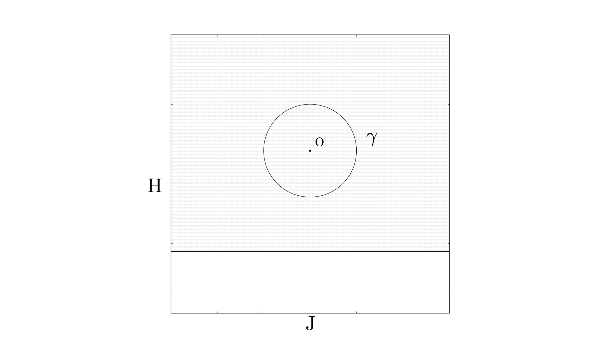
Figure 5. Bifurcation diagram of a $1$:$(-1)$ system. The set of regular values is shown gray; the critical values are colored black; the isolated critical point $O=(0,0)$ lifts to the singly pinched torus $F^{-1}(O)$.

Remark 4.4.

If $mn<0$, then the fixed point $z=w=0$ of the $\mathbb{S}^{1}$ action is necessarily at the boundary of the corresponding bifurcation diagram. Hence non-trivial monodromy (standard or fractional) can only be found when $mn>0$. Because of Theorem 4.3, non-trivial standard monodromy can manifest itself only when $m=n=1$.

Example 4.5.

An example of such a $1$:$-1$ resonant system can be obtained by considering the Hamiltonian

$$H =p_{1}q_{2}+p_{2}q_{1}+\varepsilon(q_{1}^{2}+p_{1}^{2})(q_{2}^{2}+p_{2}^{2}).$$

The bifurcation diagram of the integral map $F=(J,H)$ has the from shown in Fig. 5. From Theorem 4.3 we infer that the monodromy matrix along $\gamma$ has the form

$$\begin{pmatrix}1&1\\ 0&1\end{pmatrix}\in\textup{SL}(2,\mathbb{Z}).$$

Example 4.6.

An example of a $m$:$(-n)$ resonant system with non-trivial fractional monodromy is the specific $1$:$(-2)$ resonant system, which has been introduced in [28]. The system is obtained by considering the Hamiltonian

$$H=2q_{1}p_{1}q_{2}+(q_{1}^{2}-p_{1}^{2})p_{2}+\varepsilon R(q,p)^{2},$$

where $\varepsilon>0$ and $R=R(q,p)$ is the $1{:}(2)$ oscillator. The bifurcation diagram of the integral map $F=(J,H)$ has the form shown in Fig. 1. In this case the set of regular values is simply connected and, thus, standard monodromy is trivial. Let the curve $\gamma$ be as in Fig. 1. From Theorem 4.3 we infer that the parallel transport group $H^{0}_{1}$ is spanned by $2a$ and $b$, and that the fractional monodromy matrix has the form

$$\begin{pmatrix}1&1/2\\ 0&1\end{pmatrix}\in\textup{SL}(2,\mathbb{Q}).$$

This system is discussed in greater detail in Subsection 1.1.

4.2. A system on $S^{2}\times S^{2}$

Let $(x_{1},x_{2},x_{3})$ and $(y_{1},y_{2},y_{3})$ be coordinates in $\mathbb{R}^{3}$. The relations

$$\{x_{i},x_{j}\}=\epsilon_{ijk}x_{k},\ \{y_{i},y_{j}\}=\epsilon_{ijk}y_{k}\mbox{ and }\{x_{i},y_{j}\}=0$$

define a Poisson structure on $\mathbb{R}^{3}\times\mathbb{R}^{3}$. The restriction of this Poisson structure to $S^{2}\times S^{2}=\{(x,y)\colon|x|=|y|=1\}$ gives the canonical symplectic structure $\omega$.

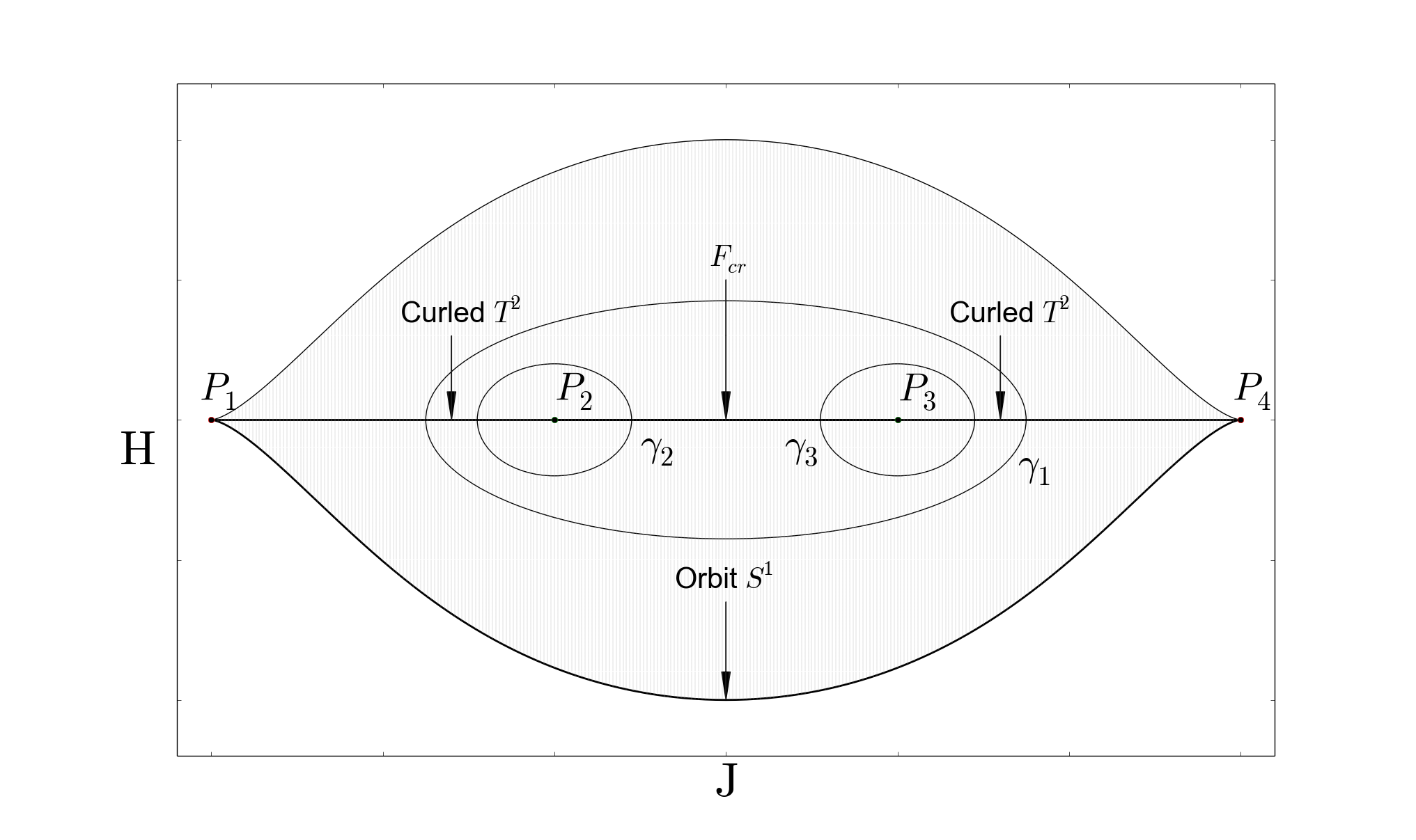
Figure 6. Bifurcation diagram of the integral map $F$. The set of regular values shown gray; the critical values are colored black. All regular fibers are $2$-tori. Curled $T^{2}$ contains one exceptional (‘short’) orbit of the $\mathbb{S}^{1}$ action. Critical fibers $F_{cr}$ contain two such orbits. They can be obtained by gluing two curled tori along a regular orbit of the $\mathbb{S}^{1}$ action.

We consider an integrable Hamiltonian system on $(S^{2}\times S^{2},\omega)$ defined by the integral map $F=(J,H)\colon S^{2}\times S^{2}\to\mathbb{R}^{2},$ where

$$J=x_{1}+2y_{1}\ \ \mbox{ and }\ \ H=\textup{Re}\{(x_{2}+ix_{3})^{2}(y_{2}-iy_{3})\}.$$

It is easily checked that the functions $J$ and $H$ commute, so $F$ is indeed an integral map. The bifurcation diagram is shown in Fig. 6.

Even without knowing the precise structure of critical fibers of $F$, we can compute fractional monodromy along curves $\gamma_{1},\gamma_{2}$ and $\gamma_{3}$, shown in Fig. 6. Specifically, assume that $\gamma_{i}(0)=\gamma_{i}(1)$ lifts to a regular torus.

Theorem 4.7.

For each $\gamma_{i}$, the parallel transport group is spanned by $2a_{i}$ and $b_{i}$, where $(a_{i},b_{i})$ forms a basis of $H_{1}(F^{-1}(\gamma_{i}(0))$ and $b_{i}$ is given by any orbit of the $\mathbb{S}^{1}$ action. The fractional monodromy matrices have the form

$$\begin{pmatrix}1&1/2\\ 0&1\end{pmatrix}\mbox{ for }\ i=2,3\ \ \mbox{ and }\ \ \begin{pmatrix}1&1\\ 0&1\end{pmatrix}\mbox{ for }\ i=1.$$

Proof. Consider the case $i=2$. The other cases can be treated analogously. The curve $\gamma_{2}$ intersects the critical line $H=0$ at two points $\xi_{1}$ and $\xi_{2}$. Let $\xi_{1}<P_{2}<\xi_{2}$ on $H=0$. The critical fiber $F^{-1}(\xi_{1})$, which is a curled torus, contains one exceptional orbit of the $\mathbb{S}^{1}$ action with $\mathbb{Z}_{2}$ isotropy. The critical fiber $F^{-1}(\xi_{1})$ contains two such orbits. Finally, observe that the point

$$(1,0,0)\times(-1,0,0)\in S^{2}\times S^{2},$$

which projects to $P_{2}$ under the map $F$, is fixed under the $\mathbb{S}^{1}$ action and has isotropy weights $m=1,n=2$. Since $F^{-1}(\gamma_{2})$ is connected, it is left to apply Theorems 3.9 and 3.12. ∎

4.3. Revisiting the quadratic spherical pendulum

The example of the system on $S^{2}\times S^{2}$ discussed in the previous Subsection 4.2 shows that fractional monodromy matrix along a given curve $\gamma_{1}$ could be an integer matrix even if standard monodromy along $\gamma_{1}$ is not defined. In this subsection we show that the same phenomenon can appear when the isotropy groups are either trivial or $\mathbb{S}^{1},$ that is, when the $\mathbb{S}^{1}$ action is free outside fixed points.

Consider a particle moving on the unit sphere

$$\{x=(x_{1},x_{2},x_{3})\in\mathbb{R}^{3}\colon x_{1}^{2}+x_{2}^{2}+x_{3}^{2}=1\}$$

in a quadratic potential $V(x_{3})=bx_{3}^{2}+cx_{3}$. The corresponding Hamiltonian system $(TS^{2},\Omega|_{TS^{2}},H)$, where $H(x,v)=\frac{1}{2}\langle v,v\rangle+V(x)$ is the total energy, is called quadratic spherical pendulum [14]. This system is completely integrable since the $x_{3}$ component $J$ of the angular momentum is conserved. Moreover, $J$ generates a global Hamiltonian $\mathbb{S}^{1}$ action on $TS^{2}$. For a certain range of parameters $b$ and $c$ the bifurcation diagram of the integral map $F=(J,H)$ has the form shown in Fig. 7.

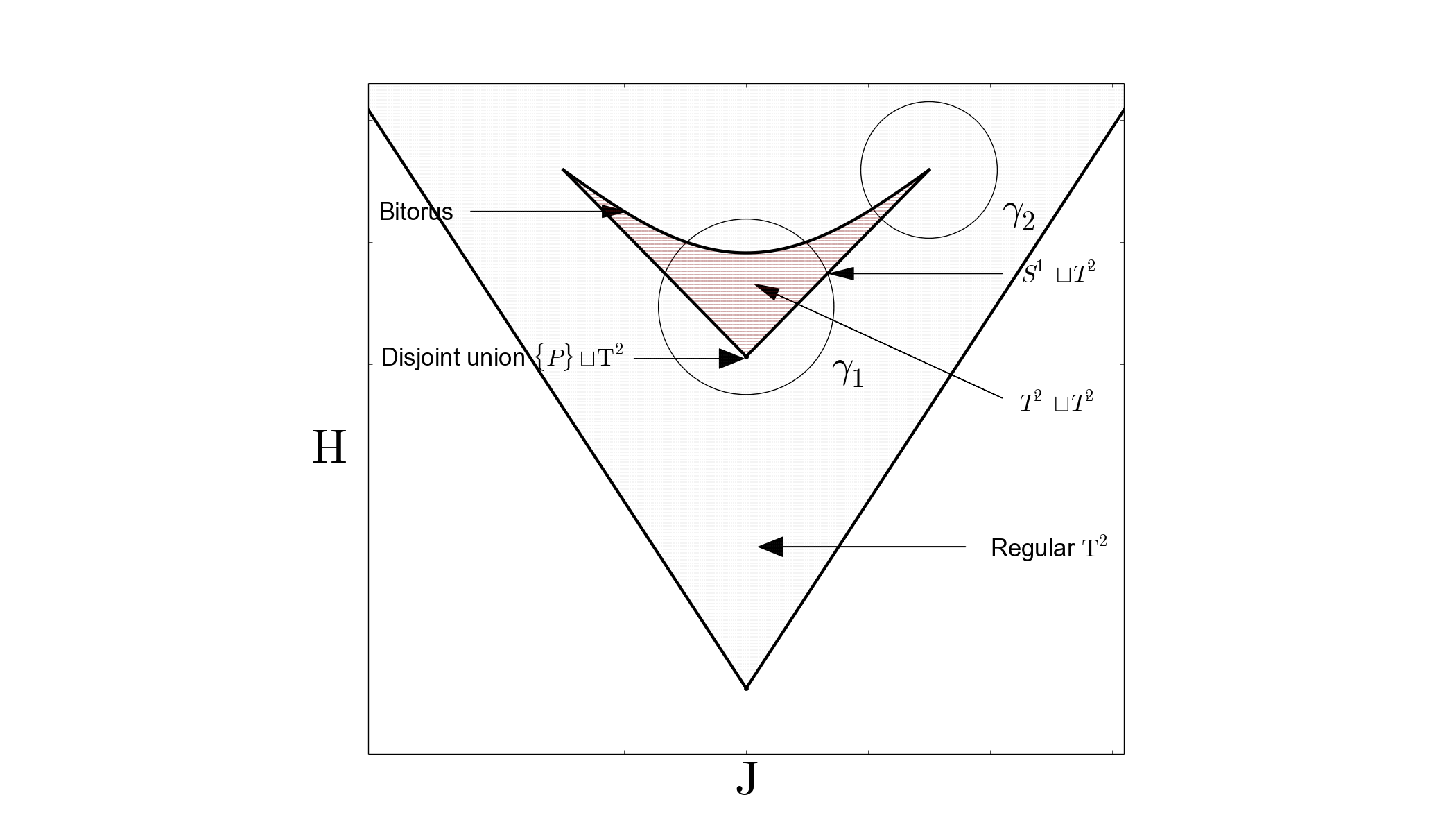
Figure 7. Bifurcation diagram of the integral map $F$. The set of regular values shown gray. The critical values are colored black. The points in the interior of the ‘island’ are regular and lift to the disjoint union of $2$ tori.

Let $\gamma_{1}$ and $\gamma_{2}$ be as in Fig. 7. Assume that the starting point $\gamma_{i}(0)=\gamma_{i}(1)$ lifts to a regular torus.

Theorem 4.8.

For each $\gamma_{i}$, the parallel transport group coincides with the whole homology group $H_{1}(F^{-1}(\gamma_{i}(0))$. The fractional monodromy matrices have the form

$$\begin{pmatrix}1&1\\ 0&1\end{pmatrix}\mbox{ for }\ i=1\ \ \mbox{ and }\ \ \begin{pmatrix}1&0\\ 0&1\end{pmatrix}\mbox{ for }\ i=2.$$

Proof. Consider the case $i=1$. The other case can be treated similarly. The $\mathbb{S}^{1}$ action is free on the connected manifold $F^{-1}(\gamma_{1})$. The Euler number of this manifold equals $1$. Indeed, the elliptic-elliptic point

$$P=(0,0,1)\times(0,0,0)\in TS^{2}\subset T\mathbb{R}^{3},$$

which projects to the point $F(P)\in\textup{int}(\gamma_{1})$, is fixed under the $\mathbb{S}^{1}$ action and has isotropy weights $m=1,n=1$. It is left to apply Theorems 3.9 and 3.12. ∎

Remark 4.9.

From Theorem 4.8 it follows that all homology cycles can be parallel transported along $\gamma_{i},\ i=1,2.$ Even though this situation is very similar to the case of standard monodromy, the monodromy along $\gamma_{i}$ is fractional. We note that such examples have not been considered until now.

5. Proof of Theorem 2.5

In the present section we use the notation introduced in Subsection 2.2. The result, Theorem 2.5, will follow from Lemmas 5.1, 5.3, 5.4, and 5.5 that are given below.

Figure 8. The base manifold $X/\mathbb{S}^{1}$.

Lemma 5.1.

There exists $k\in\mathbb{Z}$ such that $(Na_{0},Na_{1}+kb_{1})$ and $(b_{0},b_{1})$ belong to $\partial_{*}(H_{2}(X,\partial X)).$

Proof. Let $\mathbb{Z}_{N}$ be the order $N$ subgroup of $\mathbb{S}^{1}.$ The quotient $X^{\prime}=X/\mathbb{Z}_{N}$, which is given by the induced action of the subgroup $\mathbb{Z}_{N}$, is the total space of the principal circle bundle

$$\Pr{{}^{\prime}}\colon X^{\prime}\to X/\mathbb{S}^{1}.$$

We note that this bundle is, moreover, trivial. Indeed, the base $X/\mathbb{S}^{1}$ has a boundary and is, thus, homotopy equivalent to a graph.

Let $b_{i}^{r}=b_{i}/\mathbb{Z}_{N},\ i=0,1$. Then $(a_{i},b_{i}^{r})$ forms a basis of $H_{1}(X_{i}/\mathbb{Z}_{N})$. There is a unique parallel transport of the cycles $a_{0}$ and $b^{r}_{0}$ along $X^{\prime}$. Indeed, take a global section $s\colon X^{\prime}/\mathbb{S}^{1}\to X^{\prime}$ with $s(X_{0}/\mathbb{S}^{1})=a_{0}.$ Then $S=s(X^{\prime}/\mathbb{S}^{1})$ is a relative $2$-cycle that gives the parallel transport of $a_{0}$. In order to transport the cycle $b_{0}^{r}$ take a smooth curve $\Gamma\subset X/\mathbb{S}^{1}$ connecting $X_{0}/\mathbb{S}^{1}$ with $X_{1}/\mathbb{S}^{1}$ and define the relative $2$-cycle by $(\Pr{{}^{\prime}})^{-1}(\Gamma).$

Remark 5.2.

In what follows we assume that $\Gamma$ is a simple curve that does not contain the singular points $\Pr(\mathfrak{p}_{1}),\ldots,\Pr(\mathfrak{p}_{M}),$ where $\Pr\colon X\to X/\mathbb{S}^{1}$ is the canonical projection; see Fig. 8.

From above it follows that the parallel transport in the reduced space has the form $a_{0}\mapsto a_{1}+kb_{1}^{r}$ and $b_{0}^{r}\mapsto b_{1}^{r}$ for some $k\in\mathbb{Z}$. The parallel transport of the cycles $(a_{0},b_{0}^{r})$ in the reduced space lifts to the parallel transport of the cycles $(Na_{0},b_{0})$ along $X$ in the original space. Indeed, let $\pi\colon X\to X^{\prime}$ be the quotient map, given by the action of $\mathbb{Z}_{N}$. The preimage

$$\pi^{-1}((\Pr{{}^{\prime}})^{-1}(\Gamma))=\Pr{{}^{-1}}(\Gamma)$$

transports $b$ since $\Gamma$ does not contain the singular points $\Pr(\mathfrak{p}_{j})$. In order to transport $Na$ take $\pi^{-1}(S).$ Since $\pi\colon\pi^{-1}(S)\to S$ is a branched $N$-covering, see Fig. 9, the preimage $\pi^{-1}(S)$ is a relative $2$-cycle that transports $Na$. The result follows. ∎

Figure 9. An example of the covering map $\pi\colon\pi^{-1}(S)\to S$. Here the Seifert manifold $X$ contains only one exceptional orbit with $\mathbb{Z}_{2}$ isotropy ($N=2$); the base $X/\mathbb{S}^{1}\cong S$ is a ‘cone with a hole’.

This following lemma shows that the parallel transport along $X$ is unique.

Lemma 5.3.

Suppose that $(0,c)\in\partial_{*}(H_{2}(X,\partial X))$ for some $c\in H_{1}(X_{1})$. Then we have $c=0$.

Proof. This statement was essentially proved in [15] (see §7.1 therein). For the sake of completeness we provide a proof below.

Since $X$ is an orientable $3$-manifold, the rank of the image $\partial_{*}(H_{2}(X,\partial X))$ is half of the rank of $H_{1}(\partial X)\simeq\mathbb{Z}^{2}\oplus\mathbb{Z}^{2}$. Hence

$$\textup{rk}\ \partial_{*}(H_{2}(X,\partial X))=2.$$

As a subgroup of a free abelian group $H_{1}(\partial X)$, the image $\partial_{*}(H_{2}(X,\partial X))$ is a free abelian group and thus is isomorphic to $\mathbb{Z}\oplus\mathbb{Z}$.

From Lemma 5.1 we get that $\alpha=(Na_{0},Na_{1}+kb_{1})$ and $\beta=(b_{0},b_{1})$ belong to $\partial_{*}(H_{2}(X,\partial X))$.

Suppose that parallel transport along $X$ is not unique. Then there exists an element $\eta=(0,c)\in\partial_{*}(H_{2}(X,\partial X))$ with $c\neq 0.$ Since $\alpha$ and $\beta$ are linearly independent over $\mathbb{Z}$, we get $l_{1}\alpha+l_{2}\beta=l_{3}\eta$, where $l_{j}$ are integers and $l_{3}\neq 0$. But $l_{1}Na_{0}+l_{2}b_{0}=0$, so $l_{1}=l_{2}=0$ and we get a contradiction. ∎

The set $H^{0}_{1}$ of cycles $\alpha\in H_{1}(X_{0})$ that can be parallel transported along $X$ forms a subgroup of $H_{1}(X_{0})$. Since $Na_{0}$ and $b_{0}$ can be parallel transported along $X$, the group $H^{0}_{1}$ is spanned by $La_{0}$ and $b_{0}$ for some $L\in\mathbb{N}$, which divides $N$. Our goal is to prove that $L=N$. The proof of this equality is based on the important Lemma 5.4 below.

Let $E$ be a closed Seifert manifold which is obtained from $X$ by identifying the boundary tori $X_{i}$ via an orbit preserving diffeomorphism that sends $a_{0}$ to $a_{1}$ and $b_{0}$ to $b_{1}$.

Lemma 5.4.

The Euler number $e(E)$ of the Seifert manifold $E$ satisfies $e(E)=\frac{k}{N}$.

Proof. Consider the action of the quotient circle $\mathbb{S}^{1}/\mathbb{Z}^{N}$ on the quotient space $E^{\prime}=E/\mathbb{Z}^{N}$. Since $E^{\prime}$ is a manifold and the action is free, we have a principal bundle $(E^{\prime},B=E/\mathbb{S}^{1},\Pr{{}^{\prime}})$. Let

$$U_{1}\cong[0,\varepsilon]\times S^{1}$$

be a cylindrical neighborhood of $X_{0}/\mathbb{S}^{1}$ in $X/\mathbb{S}^{1}$ with $\{0\}\times S^{1}\cong X_{0}/\mathbb{S}^{1}.$ Define

$$U_{2}=\overline{B\setminus U_{1}}.$$

We already know that if $X^{\prime}=X/\mathbb{Z}_{N}$ then $(X^{\prime},X/\mathbb{S}^{1},\Pr{{}^{\prime}})$ is a trivial circle bundle. Observe that $E^{\prime}$ is obtained from $X^{\prime}$ by identifying the boundary tori $X^{\prime}_{0}$ and $X^{\prime}_{1}$ via a diffeomorphism induced by the ‘monodromy’ matrix $\begin{pmatrix}1&k\\ 0&1\end{pmatrix}$. Hence there exist cross sections $s_{1}\colon U_{1}\to E^{\prime}$ and $s_{2}\colon U_{2}\to E^{\prime}$ such that $s_{2}=s_{1}$ on the boundary circle $\{\varepsilon\}\times S^{1}$ and $s_{1}=e^{ik\varphi}s_{2}$ on $\{0\}\times S^{1}$, parametrized by an angle $\varphi$.

Let $f\colon[0,2\pi]\to[0,1]$ be a smooth function such that $f|_{[0,\delta]}=1$ and $f|_{[2\delta,2\pi]}=0$. Define a continuous function $h\colon[0,\varepsilon]\times S^{1}\to[0,2\delta]$ by the following formula

$$h(\phi,\varphi)=\dfrac{\varepsilon-\phi}{\varepsilon}\varphi f(\varphi).$$

Let $D^{2}=(0,\varepsilon)\times(\delta,2\pi).$ Define new cross sections $s^{\prime}_{1}\colon U_{1}\to E^{\prime}$ and $s^{\prime}_{2}\colon B\setminus D^{2}\to E^{\prime}$ as follows

$$s^{\prime}_{1}=s_{1}\cdot e^{ikh}\ \ \ \mbox{ and }\ \ \ s^{\prime}_{2}=\begin{cases}s_{2}&\text{on $U_{2}$,}\\ s^{\prime}_{1}&\text{otherwise.}\end{cases}$$

Observe that $s_{1}(0\times S^{1})=s_{2}(0\times S^{1})+kb,$ where $b$ corresponds to the $\mathbb{S}^{1}$ action. If $\delta>0$ is small enough, then $s_{1}(0\times S^{1})$ is homological to $s^{\prime}_{1}(0\times S^{1}).$ Hence

$$s^{\prime}_{1}(0\times S^{1})=s^{\prime}_{2}(0\times S^{1})+kb.$$

But $s^{\prime}_{1}(\partial D^{2}+0\times S^{1})=s^{\prime}_{2}(\partial D^{2}+0\times S^{1})$. Therefore

$$s^{\prime}_{2}(\partial D^{2})=s^{\prime}_{1}(\partial D^{2})+kb.$$

Thus, $e(E^{\prime})=k$ and

$$e(E)=\frac{1}{N}e(E^{\prime})=\dfrac{k}{N}.$$

∎

Lemma 5.5.

The parallel transport group $H^{0}_{1}$ is spanned by the cycles $Na_{0}$ and $b_{0}$.

Proof. We have already noted that $H^{0}_{1}$ is spanned by $La_{0}$ and $b_{0}$ for some $L\in\mathbb{N}$, which divides $N$. In order to prove the equality $L=N$ it is sufficient to prove that for every $j$ the number $L$ is a multiple of $n_{j}$ (the order of the exceptional orbit $\mathfrak{p}_{j}$).

The image of the exceptional fiber $\mathfrak{p}_{j}$ under the projection $\Pr\colon E\to B=E/\mathbb{S}^{1}$ is a single point $\Pr(\mathfrak{p}_{i})$ on the base manifold $B$. Cutting $E$ along the torus $X_{0}\cong X_{1}$ results in the manifold $X$. The quotient $X/\mathbb{S}^{1}$ is obtained from $B$ by cutting along an embedded circle. Consider an annulus $A_{j}\subset X/\mathbb{S}^{1}$ that contains $X_{0}/\mathbb{S}^{1}$ and exactly one singular point $\Pr(\mathfrak{p}_{j})$; see Fig 8.

Clearly, the preimage $E_{j}=\Pr^{-1}(A_{j})$ is a Seifert manifold with only one exceptional fiber. From the definition of the parallel transport it follows that there exists a relative cycle $S\subset E_{j}$ such that one of the connected components of $S$ is $La_{0}$. In other words, $La_{0}$ can be parallel transported along $E_{j}$.

Let us identify the boundary tori of $E_{j}$ via an orbit preserving diffeomorphism. Then the result of the parallel transport of $La_{0}$ along $E_{j}$ is $l_{1}a_{0}+l_{2}b_{0}$. Since the parallel transport is unique, see Lemma 5.3, we have

(5) $$Nl_{1}a_{0}+Nl_{2}b_{0}=NLa_{0}=LNa_{0}=LNa_{0}+Lm_{j}b_{0},$$

where $m_{j}\in\mathbb{Z}.$ Let $e_{j}$ denote the Euler number of the Seifert manifold $E_{j}$. From Lemma 5.4 it follows that

$$m_{j}/n_{j}=e_{j}\pmod{1}.$$

In particular, $m_{j}$ and $n_{j}$ are relatively prime. Eq. (5) implies $Nl_{2}=Lm_{j}$. Since $n_{j}$ divides $N$, it also divides $L$. ∎

6. Discussion

In [17] we have shown that if the circle action is free outside isolated fixed points then standard monodromy can be completely determined by the weights $1{:}(\pm 1)$ of the circle action at those points. This result allowed us to consider both focus-focus and elliptic-elliptic singular points of the integral map and provide a unified result for standard monodromy around such points. Moreover, it showed that the circle action is more important for determining standard monodromy than the precise form of the integral map $F$.

In the present paper we generalized results from [17] to the setting of Seifert fibrations. Specifically, we showed that the parallel transport along the total space of such a fibration is well defined and is completely determined by the Euler number and the orders of the exceptional orbits. Then, we applied the obtained results to fractional monodromy in singular Lagrangian fibrations (integrable Hamiltonian systems) that are invariant under an effective (Hamiltonian) circle action with isolated fixed points.

In the case of singular Lagrangian fibrations fixed points with weights $m{:}n$ different from $1{:}(\pm 1)$ may appear. The existence of such weights $m{:}n$ implies the existence of points with non-trivial isotropy group $\mathbb{Z}_{m}$ or $\mathbb{Z}_{n}$. Such points are projected to one-parameter families of critical values of $F$. These families contain essential information about the geometry of the singular Lagrangian fibration. However, for standard monodromy such critical families are ‘invisible’ in the sense that in standard monodromy we only consider the regular part of the fibration and the curves $\gamma$ along which standard monodromy is defined do not cross any critical values. In the fractional case the curves $\gamma$ are allowed to cross critical values of $F$. Our results show that also in this fractional case the circle action is more important for fractional monodromy than the precise form of the integral map $F$.

References

- [1] V. I. Arnol’d and A. Avez, Ergodic problems of classical mechanics, W.A. Benjamin, Inc., 1968.
- [2] M. Audin, Torus actions on symplectic manifolds, Birkhäuser, 2004.
- [3] L. M. Bates, Monodromy in the champagne bottle, Journal of Applied Mathematics and Physics (ZAMP) 42 (1991), no. 6, 837–847.
- [4] L. M. Bates and M. Zou, Degeneration of hamiltonian monodromy cycles, Nonlinearity 6 (1993), no. 2, 313–335.
- [5] S. Bochner, Compact groups of differentiable transformations, Ann. of Math. 46 (1945), no. 3, 372–381.
- [6] A.V. Bolsinov, Izosimov A.M., A.Y. Konyaev, and A.A. Oshemkov, Algebra and topology of integrable systems. Research problems (in Russian), Trudy Sem. Vektor. Tenzor. Anal. 28 (2012), 119–191.
- [7] A.V. Bolsinov and A.T. Fomenko, Integrable hamiltonian systems: Geometry, topology, classification, CRC Press, 2004.
- [8] H.W. Broer, K. Efstathiou, and O.V. Lukina, A geometric fractional monodromy theorem, Discrete and Continuous Dynamical Systems 3 (2010), no. 4, 517–532.
- [9] R. H. Cushman and L. M. Bates, Global aspects of classical integrable systems, 2 ed., Birkhäuser, 2015.
- [10] R. H. Cushman and H. Knörrer, The energy momentum mapping of the Lagrange top, Differential Geometric Methods in Mathematical Physics, Lecture Notes in Mathematics, vol. 1139, Springer, 1985, pp. 12–24.
- [11] R.H. Cushman and D.A. Sadovskií, Monodromy in the hydrogen atom in crossed fields, Physica D: Nonlinear Phenomena 142 (2000), no. 1-2, 166–196.
- [12] J. J. Duistermaat, On global action-angle coordinates, Communications on Pure and Applied Mathematics 33 (1980), no. 6, 687–706.
- [13] by same author, The monodromy in the hamiltonian hopf bifurcation, Zeitschrift für Angewandte Mathematik und Physik (ZAMP) 49 (1998), no. 1, 156.
- [14] K. Efstathiou, Metamorphoses of Hamiltonian systems with symmetries, Springer, Berlin Heidelberg New York, 2005.
- [15] K. Efstathiou and H. W. Broer, Uncovering fractional monodromy, Communications in Mathematical Physics 324 (2013), no. 2, 549–588.
- [16] K. Efstathiou, R.H. Cushman, and D.A. Sadovskií, Fractional monodromy in the 1:−2 resonance, Advances in Mathematics 209 (2007), no. 1, 241 – 273.
- [17] K. Efstathiou and N. Martynchuk, Monodromy of Hamiltonian systems with complexity-1 torus actions, Geometry and Physics 115 (2017), 104–115.
- [18] A. T. Fomenko and S. V. Matveev, Algorithmic and computer methods for three-manifolds, 1st ed., Springer Netherlands, 1997.
- [19] A.T. Fomenko and H. Zieschang, Topological invariant and a criterion for equivalence of integrable Hamiltonian systems with two degrees of freedom., Izv. Akad. Nauk SSSR, Ser. Mat. 54 (1990), no. 3, 546–575 (Russian).
- [20] A. Giacobbe, Fractional monodromy: Parallel transport of homology cycles, Diff. Geom. and Appl. 26 (2008), 140–150.
- [21] A. Hatcher, Notes on basic 3-manifold topology, Available online, 2000.
- [22] M. Jankins and W.D. Neumann, Lectures on seifert manifolds, Brandeis lecture notes, Brandeis University, 1983.
- [23] L. M. Lerman and Ya. L. Umanskiĭ, Classification of four-dimensional integrable Hamiltonian systems and Poisson actions of in extended neighborhoods of simple singular points. i, Russian Academy of Sciences. Sbornik Mathematics 77 (1994), no. 2, 511–542.
- [24] O. V. Lukina, F. Takens, and H. W. Broer, Global properties of integrable hamiltonian systems, Regular and Chaotic Dynamics 13 (2008), no. 6, 602–644.
- [25] V. S. Matveev, Integrable Hamiltonian system with two degrees of freedom. the topological structure of saturated neighbourhoods of points of focus-focus and saddle-saddle type, Sbornik: Mathematics 187 (1996), no. 4, 495–524.
- [26] N. N. Nekhoroshev, Action-angle variables, and their generalizations, Trans. Moscow Math. Soc. 26 (1972), 181–198.
- [27] by same author, Fractional monodromy in the case of arbitrary resonances, Sbornik: Mathematics 198 (2007), no. 3, 383–424.
- [28] N.N. Nekhoroshev, D.A. Sadovskií, and B.I. Zhilinskií, Fractional Hamiltonian monodromy, Annales Henri Poincaré 7 (2006), 1099–1211.
- [29] D. A. Sadovskií and B. I. Zhilinskií, Monodromy, diabolic points, and angular momentum coupling, Physics Letters A 256 (1999), no. 4, 235–244.
- [30] S. Schmidt and H. R. Dullin, Dynamics near the resonance, Physica D: Nonlinear Phenomena 239 (2010), no. 19, 1884–1891.
- [31] D. Sugny, P. Mardešić, M. Pelletier, A. Jebrane, and H. R. Jauslin, Fractional hamiltonian monodromy from a gauss–manin monodromy, Journal of Mathematical Physics 49 (2008), no. 4, 042701.
- [32] D.I. Tonkonog, A simple proof of the geometric fractional monodromy theorem, Moscow University Mathematics Bulletin 68 (2013), no. 2, 118–121.
- [33] H. Waalkens, H. R. Dullin, and P. H. Richter, The problem of two fixed centers: bifurcations, actions, monodromy, Physica D: Nonlinear Phenomena 196 (2004), no. 3-4, 265–310.
- [34] H. Waalkens, A. Junge, and H. R. Dullin, Quantum monodromy in the two-centre problem, Journal of Physics A: Mathematical and General 36 (2003), no. 20, L307.
- [35] N. T. Zung, A note on focus-focus singularities, Differential Geometry and its Applications 7 (1997), no. 2, 123–130.