Deconstruction and conditional erasure of quantum correlations

Abstract

We define the deconstruction cost of a tripartite quantum state on systems $ABE$ as the minimum rate of noise needed to apply to the $AE$ systems, such that there is negligible disturbance to the marginal state on the $BE$ systems, while the system $A$ of the resulting state is locally recoverable from the $E$ system alone. We refer to such actions as deconstruction operations and protocols implementing them as state deconstruction protocols. State deconstruction generalizes Landauer erasure of a single-party quantum state as well the erasure of correlations of a two-party quantum state. We find that the deconstruction cost of a tripartite quantum state on systems $ABE$ is equal to its conditional quantum mutual information (CQMI) $I(A;B|E)$, thus giving the CQMI an operational interpretation in terms of a state deconstruction protocol. We also define a related task called conditional erasure, in which the goal is to apply noise to systems $AE$ in order to decouple system $A$ from systems $BE$, while causing negligible disturbance to the marginal state of systems $BE$. We find that the optimal rate of noise for conditional erasure is also equal to the CQMI $I(A;B|E)$. State deconstruction and conditional erasure lead to operational interpretations of the quantum discord and squashed entanglement, which are quantum correlation measures based on the CQMI. We find that the quantum discord is equal to the cost of simulating einselection, the process by which a quantum system interacts with an environment, resulting in selective loss of information in the system. The squashed entanglement is equal to half the minimum rate of noise needed for deconstruction/conditional erasure if Alice has available the best possible system $E$ to help in the deconstruction/conditional erasure task.

LABEL:FirstPage1 LABEL:LastPage#110

I Introduction

The Landauer erasure principle represents a deep link between information theory and thermodynamics L61 . An informal summary of the principle is that the work cost of erasing the contents of a computer memory is proportional to the amount of information stored there. This insight has now sparked a whole literature, a consequence of which has been a deepening of the connection between information theory and thermodynamics (see, e.g., GHRRS15 for a review).

One generalization of Landauer’s insight goes beyond the single-system setup mentioned above. In GPW05 , Groisman et al. considered a setting in which two parties share a quantum state $\rho_{AB}$. Their goal was to determine the work cost of erasing the correlations present in the state, by acting locally on one system, such that the resulting state has a tensor-product form $\sigma_{A}\otimes\omega_{B}$, where $\sigma_{A}$ and $\omega_{B}$ are quantum states. Groisman et al. solved the problem in the framework of quantum Shannon theory W16 , whereby they allowed the two parties to have many copies of the state $\rho_{AB}$ and quantified the minimum rate of noise that needs to be applied to the $A$ systems such that the resulting state is tensor-product between the $A$ systems and the $B$ systems. They found that the optimal rate of noise is equal to the quantum mutual information of the state $\rho_{AB}$, defined as

$$I(A;B)_{\rho}\equiv H(A)_{\rho}+H(B)_{\rho}-H(AB)_{\rho},$$ (1)

where the quantum entropy of a state $\sigma_{G}$ on system $G$ is defined as $H(G)_{\sigma}\equiv-\operatorname{Tr}\{\sigma_{G}\log_{2}\sigma_{G}\}$. An important consequence of their theorem is that we can assign a physical meaning to, or operational interpretation of, the quantum mutual information as the minimum rate of noise needed to completely erase the correlations present in a two-party quantum state. Thus, we can say that quantum mutual information is equal to the work cost of correlation destruction.

On the other hand, quantum mutual information has also been interpreted in a communication-theoretic task (now called coherent state merging O08a ) as the optimal rate of entanglement creation when transferring the system $A$ of $\rho_{AB}$ to a party possessing system $B$ ADHW06FQSW , while using quantum communication at a fixed rate. These dual interpretations of quantum mutual information in terms of destruction and creation perhaps come at no surprise if one is familiar with the unitarity of quantum mechanics and the purification principle. Information can never truly be destroyed in quantum mechanics, which means that the apparent destruction of correlations between two parties implies the creation of correlations elsewhere, i.e., with another party who possesses a purification of the state $\rho_{AB}$. In fact, this insight is the main idea underlying the decoupling principle qip2002schu ; qcap2008first , which is a method for proving the above theorem ADHW06FQSW  and others similar to it.

In this paper, we are interested in further generalizations of the erasure of correlations to a three-system scenario, i.e., for a tripartite quantum state $\rho_{ABE}$ (see also our companion paper BBMW18 ). The tasks we are interested in accomplishing are more delicate than the destruction of correlations mentioned above.

The first task we consider is a state deconstruction protocol, whose aim is to deconstruct (literally, “to break into constituent components”) the correlations in a three-party quantum state. To make the setting precise, consider a state $\rho_{ABE}$, and suppose that Alice possesses system $A$, Bob system $B$, and Eve system $E$. We would like a deconstruction protocol to result in a state for which Eve is the mediator of correlations between Alice and Bob, while the original correlations shared between Eve and Bob are negligibly disturbed. The setup begins with Alice and Eve in the same laboratory and Bob in a different laboratory, and we also operate in the framework of quantum Shannon theory, allowing them to share $n$ copies of the state $\rho_{ABE}$, where $n$ can be a large number. Following Groisman et al. GPW05 , we allow for a local unitary randomizing channel acting on the $AE$ systems and an ancilla. The rate of noise is equal to the logarithm of the number of unitaries in such a channel divided by the number $n$ of copies of the state $\rho_{ABE}$. We define the deconstruction cost of a tripartite state $\rho_{ABE}$ to be the minimum rate of noise needed to apply to the $AE$ systems and an ancilla, such that the resulting state satisfies the following:

1. the resulting system of Alice is locally recoverable from Eve’s system alone, and

2. the correlations between Eve and Bob are negligibly disturbed.

See Section IV.1 for a more detailed definition and Figure 2 for a depiction of a state deconstruction protocol along with the conditions of local recoverability and negligible disturbance.

The second task we consider is conditional erasure. Such a task is very similar to state deconstruction: we allow for a local channel to act on the $AE$ systems and an ancilla. However, we define the conditional erasure cost to be the minimum rate of noise such that the resulting system of Alice is decoupled from the $BE$ systems and the marginal state of the $BE$ systems is negligibly disturbed. A protocol that accomplishes conditional erasure also accomplishes state deconstruction: this is because a decoupled system is locally recoverable.

The negligible disturbance condition is critical in both state deconstruction and conditional erasure: it could be the case that Eve and Bob would want to use their systems for some later quantum information processing task, so that keeping the correlations intact is essential for the systems to be useful later on. For example, Eve’s and Bob’s systems might contain some entanglement which could be useful for a subsequent distributed quantum computation. This condition also highlights an essential difference between semi-classical and fully quantum protocols: in the case that the system $E$ is classical, the negligible disturbance condition is not necessary because one could always observe the value in Eve’s system without causing any disturbance to it. However, in the quantum case, the uncertainty principle forbids us from taking a similar action, so that it is necessary for fully quantum protocols to proceed with a greater sleight of hand.

State deconstruction and conditional erasure are far more delicate than decoupling, the latter sometimes described as having the “relatively indiscriminate goal of destruction” ADHW06FQSW . That is, a naive application of the decoupling method is too blunt of a tool to apply in these protocols. Applying it naively would result in the annihilation of correlations such that if correlations between systems $B$ and $E$ were present beforehand, they would be destroyed and thus no longer useful for a future quantum information processing task.

II Main result

The main result of this paper is that both the deconstruction cost and the conditional erasure cost of a tripartite state $\rho_{ABE}$ are equal to its conditional quantum mutual information (CQMI), defined as

$$I(A;B|E)_{\rho}\equiv I(AE;B)_{\rho}-I(E;B)_{\rho}.$$ (2)

(See Theorems 4 and 7.) Thus, our result assigns a new physical meaning to the CQMI, in terms of erasure or thermodynamical tasks that generalize Landauer’s original scenario as well as the erasure of correlations scenario from GPW05 . The deconstruction and conditional erasure tasks are intimately related to properties of the CQMI itself, which has previously been related to local recoverability HJPW04 ; FR14 ; BSW14  as well as the condition of negligible disturbance WDHW13 .

The state deconstruction and conditional erasure tasks are also closely related to the protocol of quantum state redistribution DY08 ; YD09 , which, prior to our contribution, was the only protocol giving an operational meaning for the CQMI. A quantum state redistribution protocol begins with many independent copies of a four-party pure state $\psi_{ABER}$, with a sender possessing the $A$ and $E$ systems, a receiver possessing the $R$ systems, and the sender and receiver sharing noiseless entanglement before communication begins. The main result of DY08 ; YD09 is that the optimal rate of quantum communication needed to redistribute the $A$ systems from the sender to the receiver is equal to $\tfrac{1}{2}I(A;B|R)_{\psi}$. In the present paper, the state redistribution protocol is one of the main tools that we use for establishing that the deconstruction and conditional erasure costs are each equal to the CQMI.

The other main tool that we use is a quantity known as the fidelity of recovery of a tripartite state $\rho_{ABE}$ SW14 :

$$F(A;B|E)_{\rho}\equiv\sup_{\mathcal{R}_{E\rightarrow AE}}F(\rho_{ABE},\mathcal{R}_{E\rightarrow AE}(\rho_{BE})),$$ (3)

where the quantum fidelity between states $\omega$ and $\tau$ is defined as $F(\omega,\tau)\equiv\left\|\sqrt{\omega}\sqrt{\tau}\right\|_{1}^{2}$ U73 and the supremum is with respect to all recovery channels $\mathcal{R}_{E\rightarrow AE}$.

Our main results then lead to operational interpretations of quantum correlation measures based on CQMI, including quantum discord Z00 ; zurek01 and squashed entanglement CW04 . We find that the quantum discord is equal to the optimal rate of simulating einselection Z03 , the process by which a system interacts with an environment in such a way as to cause selective loss of information in the system. In particular, given a bipartite state $\rho_{AB}$ and measurement $\Lambda_{A}$, we find that the discord is equal to the minimum rate of noise needed to apply to the $A$ system of $\rho_{AB}$, such that the resulting state is locally recoverable after performing a measurement on the $A$ system and its post-measurement state is indistinguishable from the post-measurement state after $\Lambda_{A}$ acts on $\rho_{AB}$. We find that the squashed entanglement of a state $\rho_{AB}$ is equal to half the minimum rate of noise needed in a deconstruction operation which has the best possible quantum side information in system $E$ to help in the deconstruction task.

An outline of the rest of the paper is as follows. In Section III, we provide more background on quantum information basics and the conditional quantum mutual information, and we review the state redistribution protocol in more detail. Section IV.1 defines a state deconstruction protocol and the deconstruction cost of a tripartite state $\rho_{ABE}$, and Section IV.2 discusses a slightly different model for state deconstruction. In Section V, we prove that the deconstruction cost is bounded from below by the CQMI. After that, Section VI proves the other inequality, by showing how a state redistribution protocol leads to one for state deconstruction. In Section VII, we define the conditional erasure task and show how a conditional erasure protocol is equivalent to a quantum state redistribution protocol, in the sense that the existence of one implies the existence of the other. We then establish the CQMI as the optimal conditional erasure cost. Section VIII details how quantum discord is equal to the optimal rate of einselection simulation, and the following section gives the aforementioned operational interpretation of squashed entanglement. We finally conclude in Section X with a summary and some open questions.

III Background

III.1 Basics of quantum information

We review some basic aspects of quantum information before proceeding with the main development (see, e.g., W16  for a review). Let $\mathcal{L}(\mathcal{H})$ denote the algebra of bounded linear operators acting on a Hilbert space $\mathcal{H}$ (we consider finite-dimensional Hilbert spaces throughout this paper). Let $\mathcal{L}_{+}(\mathcal{H})$ denote the subset of positive semi-definite operators. An operator $\rho$ is in the set $\mathcal{D}(\mathcal{H})$ of density operators (or states) if $\rho\in\mathcal{L}_{+}(\mathcal{H})$ and Tr$\left\{\rho\right\}=1$. Throughout this paper, we let $\pi$ denote the maximally mixed state on a given Hilbert space $\mathcal{H}$, so that $\pi\equiv I_{\mathcal{H}}/\dim(\mathcal{H)}$. The tensor product of two Hilbert spaces $\mathcal{H}_{A}$ and $\mathcal{H}_{B}$ is denoted by $\mathcal{H}_{A}\otimes\mathcal{H}_{B}$ or $\mathcal{H}_{AB}$. Given a multipartite density operator $\rho_{AB}\in\mathcal{D}(\mathcal{H}_{A}\otimes\mathcal{H}_{B})$, we unambiguously write $\rho_{A}=\$Tr${}_{B}\left\{\rho_{AB}\right\}$ for the reduced density operator on system $A$. We use $\rho_{AB}$, $\sigma_{AB}$, $\tau_{AB}$, $\omega_{AB}$, etc. to denote general density operators in $\mathcal{D}(\mathcal{H}_{A}\otimes\mathcal{H}_{B})$, while $\psi_{AB}$, $\varphi_{AB}$, $\phi_{AB}$, etc. denote rank-one density operators (pure states) in $\mathcal{D}(\mathcal{H}_{A}\otimes\mathcal{H}_{B})$ (with it implicit, clear from the context, and the above convention implying that $\psi_{A}$, $\varphi_{A}$, $\phi_{A}$ may be mixed if $\psi_{AB}$, $\varphi_{AB}$, $\phi_{AB}$ are pure). A purification $|\phi^{\rho}\rangle_{RA}\in\mathcal{H}_{R}\otimes\mathcal{H}_{A}$ of a state $\rho_{A}\in\mathcal{D}(\mathcal{H}_{A})$ is such that $\rho_{A}=\operatorname{Tr}_{R}\{|\phi^{\rho}\rangle\langle\phi^{\rho}|_{RA}\}$. An isometry $U:\mathcal{H}\rightarrow\mathcal{H}^{\prime}$ is a linear map such that $U^{{\dagger}}U=I_{\mathcal{H}}$. Often, an identity operator is implicit if we do not write it explicitly (and should be clear from the context).

A linear map $\mathcal{N}_{A\rightarrow B}:\mathcal{L}(\mathcal{H}_{A})\rightarrow\mathcal{L}(\mathcal{H}_{B})$ is positive if $\mathcal{N}_{A\rightarrow B}\left(\sigma_{A}\right)\in\mathcal{L}(\mathcal{H}_{B})_{+}$ whenever $\sigma_{A}\in\mathcal{L}(\mathcal{H}_{A})_{+}$. Let id_A denote the identity map acting on a system $A$. A linear map $\mathcal{N}_{A\rightarrow B}$ is completely positive if the map id${}_{R}\otimes\mathcal{N}_{A\rightarrow B}$ is positive for a reference system $R$ of arbitrary size. A linear map $\mathcal{N}_{A\rightarrow B}$ is trace-preserving if $\operatorname{Tr}\left\{\mathcal{N}_{A\rightarrow B}\left(\tau_{A}\right)\right\}=\operatorname{Tr}\left\{\tau_{A}\right\}$ for all input operators $\tau_{A}\in\mathcal{L}(\mathcal{H}_{A})$. A quantum channel is a linear map which is completely positive and trace-preserving (CPTP). A quantum channel $\mathcal{U}:\mathcal{L}(\mathcal{H}_{A})\rightarrow\mathcal{L}(\mathcal{H}_{B})$ is an isometric channel if it has the action $\mathcal{U}(X_{A})=UX_{A}U^{{\dagger}}$, where $X_{A}\in\mathcal{L}(\mathcal{H}_{A})$ and $U:\mathcal{H}_{A}\rightarrow\mathcal{H}_{B}$ is an isometry.

The trace distance between two quantum states $\rho,\sigma\in\mathcal{D}(\mathcal{H})$ is equal to $\left\|\rho-\sigma\right\|_{1}$. It has a direct operational interpretation in terms of the distinguishability of these states. That is, if $\rho$ or $\sigma$ are prepared with equal probability and the task is to distinguish them via some quantum measurement, then the optimal success probability in doing so is equal to $\left(1+\left\|\rho-\sigma\right\|_{1}/2\right)/2$. The trace distance and fidelity are related by the Fuchs-van-de-Graaf inequalities FG98 :

$$1-\sqrt{F(\rho,\sigma)}\leq\frac{1}{2}\left\|\rho-\sigma\right\|_{1}\leq\sqrt{1-F(\rho,\sigma)}.$$ (4)

The rightmost quantity above is known to be a distance measure, satisfying the triangle inequality, as proposed and shown in GLN05 . This quantity was generalized to subnormalized states and given the name “purified distance” in TCR09 .

Let $\{|i\rangle_{A}\}$ denote the standard, orthonormal basis for a Hilbert space $\mathcal{H}_{A}$, and let $\{|i\rangle_{B}\}$ be defined similarly for $\mathcal{H}_{B}$. If the dimensions of these spaces are equal ($\dim(\mathcal{H}_{A})=\dim(\mathcal{H}_{B})=d$), then we define the maximally entangled state $|\Phi\rangle_{AB}\in\mathcal{H}_{A}\otimes\mathcal{H}_{B}$ as

$$|\Phi\rangle_{AB}\equiv\frac{1}{\sqrt{d}}\sum_{i=1}^{d}|i\rangle_{A}\otimes|i\rangle_{B}.$$ (5)

The generalized Pauli shift operator $X$ is defined by $X_{A}|i\rangle_{A}=|i\oplus 1\rangle_{A}$, where addition is modulo $d$. The generalized Pauli phase operator $Z$ is defined by $Z_{A}|k\rangle_{A}=\exp(2\pi ik/d)|k\rangle_{A}$. The Heisenberg–Weyl group is defined as $\{X_{A}^{j}Z_{A}^{k}\}_{j,k\in\left\{1,\ldots,d\right\}}$, and satisfies

$$\frac{1}{d}\operatorname{Tr}\{X_{A}^{j}Z_{A}^{k}\}=\delta_{d,j}\delta_{d,k}.$$ (6)

The generalized Bell basis is defined as $\{|\Phi^{j,k}\rangle_{AB}\}_{j,k\in\left\{1,\ldots,d\right\}}$, where

$$|\Phi^{j,k}\rangle_{AB}=(X_{A}^{j}Z_{A}^{k}\otimes I_{B})|\Phi\rangle_{AB}.$$ (7)

It is an orthonormal basis as a consequence of (6).

III.2 Conditional quantum mutual information

Here we briefly provide more background on the conditional quantum mutual information (CQMI). The CQMI is understood informally as quantifying the correlations between systems $A$ and $B$ from the perspective of a party possessing system $E$ DY08 ; YD09 . The CQMI is symmetric with respect to the exchange of the $A$ and $B$ systems of a state $\rho_{ABE}$: $I(A;B|E)_{\rho}=I(B;A|E)_{\rho}$. One of the powerful properties of the CQMI is that it obeys a chain rule of the following form for a state $\sigma_{A_{1}\cdots A_{n}BE}$:

$$I(A_{1}\cdots A_{n};B|E)_{\sigma}=\sum_{i=1}^{n}I(A_{i};B|EA_{1}^{i-1})_{\sigma},$$ (8)

where $A_{1}^{i-1}\equiv A_{1}\cdots A_{i-1}$, so that we can think of the correlations between $A_{1}\cdots A_{n}$ and $B$, as observed by $E$, being built up one system at a time. The CQMI is always non-negative $I(A;B|E)_{\rho}\geq 0$, an entropy inequality known as strong subadditivity LR73 ; PhysRevLett.30.434 . A first relation of CQMI to recoverability was established in HJPW04 , in which it was shown that $I(A;B|E)_{\rho}=0$ if and only if there exists a recovery quantum channel $\mathcal{R}_{E\rightarrow AE}$ such that the global state $\rho_{ABE}$ can be reconstructed by acting on one share $E$ of the marginal state $\rho_{BE}$:

$$\rho_{ABE}=\mathcal{R}_{E\rightarrow AE}(\rho_{BE}).$$ (9)

More recently, it was shown that these results are robust FR14 ; BSW14 : the CQMI is approximately equal to zero (i.e., $I(A;B|E)_{\rho}\approx 0$) if and only if the global state is approximately recoverable by acting on one share $E$ of the marginal $\rho_{BE}$ (i.e., $\rho_{ABE}\approx\mathcal{R}_{E\rightarrow AE}(\rho_{BE})$). In more detail, FR14 established the inequality

$$I(A;B|E)_{\rho}\geq-\log F(A;B|E)_{\rho},$$ (10)

and FR14 ; BSW14 established a converse relation. Using some recent tools Winter15 and the Fuchs-van-de-Graaf inequalities in (4), the following refinement of the converse holds (W16, , Theorem 11.10.5): if $F(A;B|E)_{\rho}\geq 1-\varepsilon$ for $\varepsilon\in(0,1)$, then

$$I(A;B|E)_{\rho}\leq 2\sqrt{\varepsilon}\log\left|B\right|\\ +\left(1+\sqrt{\varepsilon}\right)h_{2}(\sqrt{\varepsilon}/\left[1+\sqrt{\varepsilon}\right]),$$ (11)

where the binary entropy $h_{2}(x)$ is defined for $x\in(0,1)$ as

$$h_{2}(x)\equiv-x\log_{2}x-\left(1-x\right)\log_{2}\left(1-x\right),$$ (12)

with the property that $\lim_{x\rightarrow 0}h_{2}(x)=0$. From the above, we see that the CQMI is a witness to quantum Markovianity: if it is small, then we can understand the correlations between $A$ and $B$ as being mediated by system $E$ via the recovery channel $\mathcal{R}_{E\rightarrow AE}$.

III.3 Quantum state redistribution

This section provides some background on quantum state redistribution DY08 ; YD09 . A quantum state redistribution protocol begins with a sender, a receiver, and a reference party sharing many independent copies of a four-system pure state $\psi_{ABER}$. The sender has the $AE$ systems, the receiver the $R$ systems, and the reference the $B$ systems. The goal is to use entanglement and noiseless quantum communication to redistribute the systems such that the sender ends up with the $E$ systems, the receiver the $AR$ systems, and the reference the $B$ systems. As a side benefit, the protocol can also generate entanglement shared between the sender and receiver at the end.

More formally, let $n\in\mathbb{N}$, $M\in\mathbb{N}$, and $\varepsilon\in\left[0,1\right]$. An $\left(n,M,\varepsilon\right)$ state redistribution protocol consists of an encoding channel $\mathcal{E}_{A^{n}E^{n}A^{\prime}\rightarrow\bar{A}_{0}A_{0}\hat{E}^{n}}$ and a decoding channel $\mathcal{D}_{\bar{A}_{0}R^{\prime}R^{n}\rightarrow\hat{A}^{n}\hat{R}^{n}R_{0}}$, such that the following state

$$\xi_{\hat{A}^{n}B^{n}\hat{E}^{n}\hat{R}^{n}A_{0}R_{0}}\equiv\mathcal{D}_{\bar{A}_{0}R^{\prime}R^{n}\rightarrow\hat{A}^{n}\hat{R}^{n}R_{0}}(\varphi_{\bar{A}_{0}A_{0}\hat{E}^{n}B^{n}R^{n}R^{\prime}}),$$ (13)

where

$$\varphi_{\bar{A}_{0}A_{0}\hat{E}^{n}B^{n}R^{n}R^{\prime}}\equiv\mathcal{E}_{A^{n}E^{n}A^{\prime}\rightarrow\bar{A}_{0}A_{0}\hat{E}^{n}}(\psi_{ABER}^{\otimes n}\otimes\Phi_{A^{\prime}R^{\prime}}),$$ (14)

has fidelity larger than $1-\varepsilon$ with the following pure state:

$$\psi_{\hat{A}B\hat{E}\hat{R}}^{\otimes n}\otimes\Phi_{A_{0}R_{0}},$$ (15)

where $\Phi_{A^{\prime}R^{\prime}}$ and $\Phi_{A_{0}R_{0}}$ denote maximally entangled states of Schmidt ranks $|A^{\prime}|$ and $|A_{0}|$, respectively. That is, an $\left(n,M,\varepsilon\right)$ state redistribution protocol satisfies

$$F(\xi_{\hat{A}^{n}B^{n}\hat{E}^{n}\hat{R}^{n}A_{0}R_{0}},\psi_{\hat{A}B\hat{E}\hat{R}}^{\otimes n}\otimes\Phi_{A_{0}R_{0}})\geq 1-\varepsilon.$$ (16)

The parameter $M$ is the dimension of the quantum system $\bar{A}_{0}$ that is communicated from sender to receiver:

$$M\equiv\left|\bar{A}_{0}\right|.$$ (17)

Definition 1 (Achievable rate)

A rate $R$ is achievable for state redistribution of $\psi_{ABER}$ if for all $\varepsilon\in\left(0,1\right)$, $\delta>0$, and sufficiently large $n$, there exists an $(n,2^{n\left[R+\delta\right]},\varepsilon)$ state redistribution protocol.

Definition 2 (Quantum comm. cost)

The quantum communication cost $\mathcal{Q}(\psi_{ABER})$ of state redistribution of $\psi_{ABER}$ is equal to the infimum of all rates which are achievable for redistribution of $\psi_{ABER}$.

The following theorem from DY08 ; YD09  gives a precise characterization of the quantum communication cost:

Theorem 1 (DY08 ; YD09 )

The quantum communication cost of state redistribution is equal to half the conditional quantum mutual information:

$$\mathcal{Q}(\psi_{ABER})=\frac{1}{2}I(A;B|R)_{\psi}.$$ (18)

The achievability part of the above theorem was simplified in PhysRevA.78.030302 , which is the formulation of state redistribution that we will use to characterize deconstruction cost.

Remark 1

The results of PhysRevA.78.030302 ; BCT16 ; DHO14  establish that the encoding channel and decoding channel for state redistribution can be chosen as unitaries, a key fact that we will use in what follows. Let $U_{A^{n}E^{n}A^{\prime}\rightarrow\bar{A}_{0}A_{0}\hat{E}^{n}}^{\mathcal{E}}$ denote the unitary encoder and $U_{\bar{A}_{0}R^{\prime}R^{n}\rightarrow\hat{A}^{n}\hat{R}^{n}R_{0}}^{\mathcal{D}}$ the unitary decoder for these protocols, and note that the state $\xi_{\hat{A}^{n}B^{n}\hat{E}^{n}\hat{R}^{n}A_{0}R_{0}}$ in (13) can be taken as a pure state as a consequence. See Figure 1 for a depiction of such a state redistribution protocol.

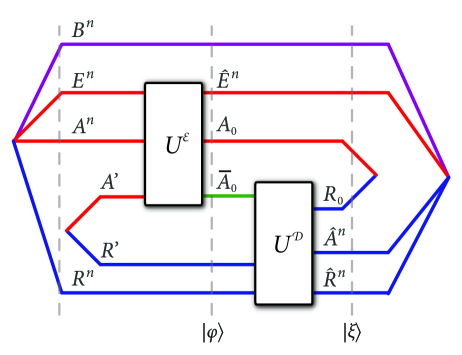
Figure 1: Quantum state redistribution with a unitary encoding and decoding. By using shared entanglement in systems $A^{\prime}$ and $R^{\prime}$ and noiseless quantum communication of the system $\bar{A}_{0}$, a sender can transfer her quantum systems $A^{n}$ to a receiver, such that the resulting state of systems $\hat{A}^{n}B^{n}\hat{R}^{n}\hat{E}^{n}$ has arbitrarily high fidelity with the initial state of systems $A^{n}B^{n}R^{n}E^{n}$. At the same time, the protocol generates entanglement in the registers $A_{0}$ and $R_{0}$.

We can also quantify the entanglement cost of a quantum state redistribution protocol. In such a case, for $L\in\mathbb{N}$, we define an $(n,M,L,\varepsilon)$ quantum state redistribution protocol specified exactly as given above, except we set

$$L\equiv|A^{\prime}|/|A_{0}|.$$ (19)

With this convention, there is an entanglement cost if $L\geq 1$ and there is an entanglement gain if $L\leq 1$. A rate pair $(R,E)$ is achievable for state redistribution of $\psi_{ABER}$ if for all $\varepsilon\in\left(0,1\right)$, $\delta>0$, and sufficiently large $n$, there exists an $(n,2^{n\left[R+\delta\right]},2^{n\left[E+\delta\right]},\varepsilon)$ state redistribution protocol. The achievable rate region of state redistribution of $\psi_{ABER}$ is equal to the union of all rate pairs which are achievable for redistribution of $\psi_{ABER}$.

Refs. DY08 ; YD09  proved that the rate pair

$$(I(A;B|R)_{\psi}/2,\left[I(A;E)_{\psi}-I(A;R)_{\psi}\right]/2)$$ (20)

is achievable and that the optimal rate region is equal to

$$R \geq\frac{1}{2}I(A;B|R)_{\psi},$$ (21)

$$R+E \geq H(A|R)_{\psi}.$$ (22)

Thus, the rate pair in (20) corresponds to an optimal corner point of the region in (21)–(22). The protocol from PhysRevA.78.030302 consumes entanglement at a rate equal to $I(A;E)_{\psi}/2$ and generates entanglement at a rate equal to $I(A;R)_{\psi}/2$.

IV State deconstruction protocol

Here we provide an operational definition for the deconstruction cost of a tripartite state $\rho_{ABE}$. We frame the problem in the formalism of quantum Shannon theory W16 , which, as we will show, ultimately leads to the CQMI being equal to the deconstruction cost after taking a limit. In what follows, we consider two seemingly different models, called the local unitary randomizing model and the Landauer–Bennett erasure model. In Section IV.3, we show that these two models are in fact equivalent to each other, in the sense that a protocol from one model can simulate a protocol from the other, with the same resource consumption and performance.

IV.1 Local unitary randomizing model

We begin by defining a state deconstruction protocol in the local unitary randomizing model. Let $n\in\mathbb{N}$, $M\in\mathbb{N}$, and $\varepsilon\in\left[0,1\right]$. An $(n,M,\varepsilon)$ state deconstruction protocol consists of an ensemble of $M$ unitaries $\{p_{i},U_{A^{n}A^{\prime}E^{n}}^{i}\}_{i=1}^{M}$ that lead to the following local unitary randomizing channel:

$$\mathcal{N}_{A^{n}A^{\prime}E^{n}}(\tau_{A^{n}A^{\prime}E^{n}})\equiv\sum_{i}p_{i}U_{A^{n}A^{\prime}E^{n}}^{i}\tau_{A^{n}A^{\prime}E^{n}}(U_{A^{n}A^{\prime}E^{n}}^{i})^{{\dagger}},$$ (23)

for a density operator $\tau_{A^{n}A^{\prime}E^{n}}$, with system $A^{\prime}$ an auxiliary system. We also refer to such an action as an $\varepsilon$-deconstruction operation and are interested in its action on the state $\rho_{ABE}^{\otimes n}\otimes\theta_{A^{\prime}}$, where $\theta_{A^{\prime}}$ is an auxiliary density operator that plays the role of a catalyst in the sense of MBDRC16  to help in the deconstruction task. The state resulting from a deconstruction operation acting on $\rho_{ABE}^{\otimes n}\otimes\theta_{A^{\prime}}$ is as follows:

$$\omega_{A^{n}A^{\prime}B^{n}E^{n}}\equiv\mathcal{N}_{A^{n}A^{\prime}E^{n}}(\rho_{ABE}^{\otimes n}\otimes\theta_{A^{\prime}}).$$ (24)

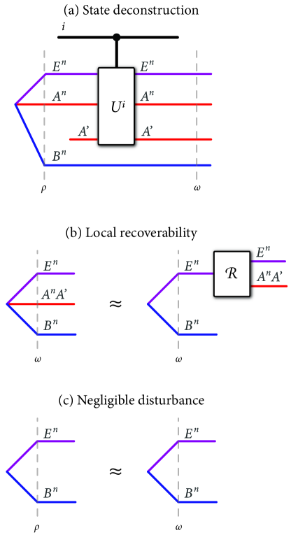
Figure 2: Depiction of (a) a state deconstruction protocol in the local unitary randomizing model along with the conditions of (b) local recoverability and (c) negligible disturbance.

We demand for such a deconstruction operation to satisfy the property of negligible disturbance and for the state resulting from the operation to be locally recoverable. In particular, the negligible disturbance condition means that the deconstruction operation $\mathcal{N}_{A^{n}A^{\prime}E^{n}}$ causes little disturbance to the residual state of the $B^{n}E^{n}$ systems, in the sense that

$$F(\omega_{B^{n}E^{n}},\rho_{BE}^{\otimes n})\geq 1-\varepsilon.$$ (25)

The condition of local recoverability means that the resulting state $\omega_{A^{n}A^{\prime}B^{n}E^{n}}$ is such that the $A^{n}A^{\prime}$ systems are locally recoverable by acting on the $E^{n}$ systems alone. That is, there exists a recovery channel $\mathcal{R}_{E^{n}\rightarrow A^{n}A^{\prime}E^{n}}$ such that

$$F(\omega_{A^{n}A^{\prime}B^{n}E^{n}},\mathcal{R}_{E^{n}\rightarrow A^{n}A^{\prime}E^{n}}(\omega_{B^{n}E^{n}}))\geq 1-\varepsilon.$$ (26)

Equivalently, we demand for the following fidelity of recovery to be large:

$$F(A^{n}A^{\prime};B^{n}|E^{n})_{\omega}\geq 1-\varepsilon.$$ (27)

Figure 2 depicts a state deconstruction protocol in the local unitary randomizing model.

Definition 3 (Achievable rate)

A rate $R$ is achievable for state deconstruction of $\rho_{ABE}$ if for all $\varepsilon\in\left(0,1\right)$, $\delta>0$, and sufficiently large $n$, there exists an $(n,2^{n\left[R+\delta\right]},\varepsilon)$ state deconstruction protocol.

Definition 4 (Deconstruction cost)

The deconstruction cost $\mathcal{D}(A;B|E)_{\rho}$ of a state $\rho_{ABE}$ is equal to the infimum of all rates which are achievable for state deconstruction of $\rho_{ABE}$.

Remark 2

(BSW14, , Proposition 35) (refined in (W16, , Theorem 11.10.5)) implies that the deconstruction cost of $\rho_{ABE}$ is equal to the minimum rate of noise needed to deconstruct the correlations in $\rho_{ABE}^{\otimes n}$ in such a way that the resulting state has vanishing normalized CQMI. Specifically, the state $\omega_{A^{n}A^{\prime}B^{n}E^{n}}$ resulting from an $\left(n,M,\varepsilon\right)$ state deconstruction protocol is such that

$$\frac{1}{n}I(A^{n}A^{\prime};B^{n}|\hat{E}^{n})_{\omega}\leq 2\sqrt{\varepsilon}\log\left|B\right|\\ +\frac{1}{n}\left(1+\sqrt{\varepsilon}\right)h_{2}(\sqrt{\varepsilon}/\left[1+\sqrt{\varepsilon}\right]).$$ (28)

Remark 3

Operational tasks related to state deconstruction were previously explored in WSM15 , where a class of “Markovianizing operations” were defined and subsequently broadened in WSM15a ; BBW15 . Deconstruction operations are different in that we allow for a catalyst, a unitary interaction between the $A^{n}E^{n}$ systems and the catalyst, and we demand for the condition of negligible disturbance to hold. Whereas our converse (Theorem 2) holds for the model of WSM15 as well, the CQMI cannot be achieved: the fact that WSM15 does not allow for an interaction with the $E$ systems leads to a strictly larger optimal rate function based on the Koashi-Imoto decomposition koashi02 (at least for pure states). This proves that the CQMI cannot be achieved without having access to the $E$ systems. The result of WSM15  is motivated from questions in distributed computation WSM15_2 but has the disadvantage that the Koashi-Imoto decomposition is not continuous in the state.

Remark 4

In Appendix B, we give a strictly classical example that demonstrates how the conditional mutual information cannot be achieved without having access to the $E$ systems.

IV.2 Landauer–Bennett erasure model

We can think of deconstruction operations in an alternative way, akin to the Landauer–Bennett model of erasure L61 ; B73  and discussed in (GPW05, , Remark II.4), in which we interact the systems of interest unitarily (reversibly) with a catalyst and subsequently perform a partial trace over some subsystem. The deconstruction cost in this case is then related to the size of the system that we trace out. In this alternative model, we define a deconstruction operation $\mathcal{N}_{A^{n}E^{n}\rightarrow A_{1}^{\prime}\hat{E}^{n}}$ as

$$\omega_{A_{1}^{\prime}B^{n}\hat{E}^{n}} \equiv\mathcal{N}_{A^{n}E^{n}\rightarrow A_{1}^{\prime}\hat{E}^{n}}(\rho_{ABE}^{\otimes n})$$ (29)

$$\equiv\operatorname{Tr}_{A_{2}^{\prime}}\{\mathcal{U}_{A^{n}E^{n}A^{\prime}\rightarrow A_{1}^{\prime}A_{2}^{\prime}\hat{E}^{n}}(\rho_{ABE}^{\otimes n}\otimes\theta_{A^{\prime}})\},$$ (30)

with $\theta_{A^{\prime}}$ an arbitrary ancilla state and $\mathcal{U}_{A^{n}E^{n}A^{\prime}\rightarrow A_{1}^{\prime}A_{2}^{\prime}\hat{E}^{n}}$ a unitary quantum channel. An $(n,M,\varepsilon)$ deconstruction protocol in this case has $n$ defined again as the number of copies of $\rho_{ABE}$ and $\varepsilon$ defined via (25) and $F(A_{1}^{\prime};B^{n}|\hat{E}^{n})_{\omega}\geq 1-\varepsilon$. However, in this Landauer–Bennett erasure model, we take $M$ defined as

$$M\equiv\left|A_{2}^{\prime}\right|^{2}.$$ (31)

In this model, we take the convention of squaring the dimension of the removed system $\left|A_{2}^{\prime}\right|^{2}$ when calculating $M$, because we are interested in measuring the amount of noise needed to remove the $A_{2}^{\prime}$ system (i.e., the amount of noise needed to physically implement a partial trace). One way to do so is to apply a randomizing channel of the following form, which realizes a partial trace:

$$\frac{1}{\left|A_{2}^{\prime}\right|^{2}}\sum_{i=1}^{\left|A_{2}^{\prime}\right|^{2}}V_{A_{2}^{\prime}}^{i}\mathcal{U}_{A^{n}E^{n}A^{\prime}\rightarrow A_{1}^{\prime}A_{2}^{\prime}\hat{E}^{n}}(\rho_{ABE}^{\otimes n}\otimes\theta_{A^{\prime}})(V_{A_{2}^{\prime}}^{i})^{{\dagger}}\\ =\pi_{A_{2}^{\prime}}\otimes\operatorname{Tr}_{A_{2}^{\prime}}\{\mathcal{U}_{A^{n}E^{n}A^{\prime}\rightarrow A_{1}^{\prime}A_{2}^{\prime}\hat{E}^{n}}(\rho_{ABE}^{\otimes n}\otimes\theta_{A^{\prime}})\},$$ (32)

where $\{V_{A_{2}^{\prime}}^{i}\}_{i=1}^{\left|A_{2}^{\prime}\right|^{2}}$ is a unitary one-design and $\pi_{A_{2}^{\prime}}\equiv I_{A_{2}^{\prime}}/|A_{2}^{\prime}|$ is the maximally mixed state. It is known that $\left|A_{2}^{\prime}\right|^{2}$ unitaries are necessary and sufficient for physically implementing a partial trace in the above sense AMTW00 .

We can then define achievable rates and the deconstruction cost for this alternative model just as in Definitions 3 and 4. This model might seem as if it is slightly different from the local unitary randomizing one, but we show in the next section that they are equivalent and thus lead to the same deconstruction cost.

IV.3 Equivalence of the two models

In this section, we show that the local unitary randomizing model and the Landauer–Bennett erasure models are equivalent, in the sense that they can simulate one another with the same performance and resource consumption. This equivalence was shown for a special case in MBDRC16 , and here we generalize the argument to the settings considered in this paper. As a consequence of our simulation argument, there is no need to consider two different notions of deconstruction cost, since the simulation argument implies that the costs are in fact the same.

First, we show that the local unitary randomizing model can simulate the Landauer–Bennett erasure model. To this end, suppose that we are given a catalyst state $\theta_{A^{\prime}}$ and an interaction unitary $U_{A^{n}E^{n}A^{\prime}\rightarrow A_{1}^{\prime}A_{2}^{\prime}\hat{E}^{n}}$, such that the Landauer–Bennett erasure deconstruction operation is as given in (30). We can simulate such an operation by choosing an ensemble of unitaries to be as follows:

$$\{1/|A_{2}^{\prime}|^{2},W_{A^{n}E^{n}A^{\prime}\rightarrow A_{1}^{\prime}A_{2}^{\prime}\hat{E}^{n}}^{i}\}_{i=1}^{|A_{2}^{\prime}|^{2}},$$ (33)

where

$$W_{A^{n}E^{n}A^{\prime}\rightarrow A_{1}^{\prime}A_{2}^{\prime}\hat{E}^{n}}^{i}\equiv V_{A_{2}^{\prime}}^{i}U_{A^{n}E^{n}A^{\prime}\rightarrow A_{1}^{\prime}A_{2}^{\prime}\hat{E}^{n}}$$ (34)

and $\{V_{A_{2}^{\prime}}^{i}\}_{i=1}^{\left|A_{2}^{\prime}\right|^{2}}$ is a set of Heisenberg–Weyl unitaries that realize a partial trace. The result is that a local unitary randomizing channel in (23) formed from the ensemble in (33) can realize the deconstruction operation in (30):

$$\frac{1}{|A_{2}^{\prime}|^{2}}\sum_{i}W^{i}(\rho_{ABE}^{\otimes n}\otimes\theta_{A^{\prime}})W^{i{\dagger}}\\ =\pi_{A_{2}^{\prime}}\otimes\operatorname{Tr}_{A_{2}^{\prime}}\{\mathcal{U}_{A^{n}E^{n}A^{\prime}\rightarrow A_{1}^{\prime}A_{2}^{\prime}\hat{E}^{n}}(\rho_{ABE}^{\otimes n}\otimes\theta_{A^{\prime}})\}\\ \equiv\pi_{A_{2}^{\prime}}\otimes\omega_{A_{1}^{\prime}B^{n}\hat{E}^{n}}.$$ (35)

Both the negligible disturbance and the local recoverability conditions hold with the same quality as in the original protocol. This is clear for the negligible disturbance condition, and to see it for the local recoverability condition, we can invoke a special case of the multiplicativity of fidelity of recovery with respect to tensor-product states BT15 :

$$F(A_{1}^{\prime}A_{2}^{\prime};B^{n}|\hat{E}^{n})_{\pi\otimes\omega}=F(A_{1}^{\prime};B^{n}|\hat{E}^{n})_{\omega}.$$ (36)

Showing the other simulation requires a bit more effort. To this end, consider an arbitrary ensemble of unitaries $\{p_{i},U_{A^{n}A^{\prime}E^{n}}^{i}\}_{i=1}^{M}$ and an ancilla $\theta_{A^{\prime}}$. We need to show how it is possible to simulate the effect of a local unitary randomizing channel of the form in (23) built from this ensemble, by bringing in an ancilla state, performing a global unitary, and ending with a partial trace. We take the ancilla to be the following state:

$$\pi_{S_{A}}\otimes\pi_{T_{A}}\otimes\sum_{i=1}^{M}p_{i}|i\rangle\langle i|_{\hat{M}_{A}}\otimes\theta_{A^{\prime}},$$ (37)

where $S_{A}$ and $T_{A}$ are quantum systems each having dimension equal to $\sqrt{M}$. (Note that if $\sqrt{M}$ is not an integer, then we can “zero-pad” the probability distribution $\{p_{i}\}$ such that its cardinality becomes a power of two—this has the negligible effect of incrementing by one the number of bits needed to describe the indices $i$ corresponding to the entries of the probability distribution $\{p_{i}\}$ and at the same time ensures that $\sqrt{M}$ is an integer). It is helpful to recall the following equality:

$$\pi_{S_{A}}\otimes\pi_{T_{A}}=\frac{1}{M}\sum_{j,k}|\Phi^{j,k}\rangle\langle\Phi^{j,k}|_{S_{A}T_{A}},$$ (38)

where $\{|\Phi^{j,k}\rangle_{S_{A}T_{A}}\}$ denotes the Bell basis reviewed in Section III.1. We take the unitary interaction between the ancilla systems $S_{A}T_{A}\hat{M}_{A}A^{\prime}$ and the data systems $A^{n}E^{n}$ to be a serial concatenation of the following two controlled unitaries:

$$\sum_{i}|i\rangle\langle i|_{\hat{M}_{A}}\otimes U_{A^{n}A^{\prime}E^{n}}^{i},$$ (39)

$$\sum_{j,k}|\Phi^{j,k}\rangle\langle\Phi^{j,k}|_{S_{A}T_{A}}\otimes X_{\hat{M}_{A}}^{(j-1)\cdot d+k}.$$ (40)

The state resulting from applying these two controlled unitaries sequentially ((39) and then (40)) to the systems $S_{A}T_{A}\hat{M}_{A}A^{n}E^{n}F$ is as follows:

$$\frac{1}{M}\sum_{j,k}|\Phi^{j,k}\rangle\langle\Phi^{j,k}|_{S_{A}T_{A}}\\ \otimes\sum_{i}p_{i}X_{\hat{M}_{A}}^{(j-1)\cdot d+k}|i\rangle\langle i|_{\hat{M}_{A}}[X_{\hat{M}_{A}}^{(j-1)\cdot d+k}]^{{\dagger}}\\ \otimes U_{A^{n}A^{\prime}E^{n}}^{i}(\rho_{ABE}^{\otimes n}\otimes\theta_{A^{\prime}})(U_{A^{n}A^{\prime}E^{n}}^{i})^{{\dagger}}.$$ (41)

After tracing over the $S_{A}$ register, which requires $\log M$ bits of noise according to our convention in (31), the state becomes as follows:

$$\pi_{T_{A}}\otimes\pi_{\hat{M}_{A}}\otimes\sum_{i}p_{i}U_{A^{n}A^{\prime}E^{n}}^{i}(\rho_{ABE}^{\otimes n}\otimes\theta_{A^{\prime}})(U_{A^{n}A^{\prime}E^{n}}^{i})^{{\dagger}}\\ \equiv\pi_{T_{A}}\otimes\pi_{\hat{M}_{A}}\otimes\omega_{A^{n}A^{\prime}B^{n}E^{n}}.$$ (42)

One can verify this explicitly, or see that it follows intuitively from a cascade: tracing over system $S_{A}$ has the effect of “forgetting” $j$ and $k$, which has the effect of randomizing the classical system $\hat{M}_{A}$ with a uniform mixture of the shift operators $X_{\hat{M}_{A}}^{(j-1)\cdot d+k}$, which in turn has the effect of “forgetting” $i$, which then applies the local unitary randomizing channel to the systems $A^{n}A^{\prime}E^{n}$. Both the negligible disturbance and the local recoverability conditions hold with the same quality as in the original protocol. This is clear for the negligible disturbance condition, and to see it for the local recoverability condition, we can invoke a special case of the multiplicativity of fidelity of recovery with respect to tensor-product states BT15 :

$$F(T_{A}\hat{M}_{A}A^{n}A^{\prime};B^{n}|E^{n})_{\pi\otimes\pi\otimes\omega}=F(A^{n}A^{\prime};B^{n}|E^{n})_{\omega}.$$ (43)

V Deconstruction cost is lower bounded by CQMI

In this section, we prove that the deconstruction cost of a tripartite state $\rho_{ABE}$ is lower bounded by its conditional quantum mutual information $I(A;B|E)_{\rho}$. We prove such a converse theorem in the Landauer–Bennett erasure model. By the simulation argument given in Section IV.3, this theorem also serves as a converse bound for deconstruction cost in the local unitary randomizing model. For the interested reader, Appendix A offers two alternative converse proofs for optimality of the deconstruction cost in the local unitary randomizing model. One of them has a flavor similar to the converse proof given below, and the other is similar to those from prior works GPW05 ; BBW15 ; WSM15a .

Theorem 2

The conditional quantum mutual information $I(A;B|E)_{\rho}$ of a tripartite state $\rho_{ABE}$ is a lower bound on its deconstruction cost $\mathcal{D}(A;B|E)_{\rho}$:

$$I(A;B|E)_{\rho}\leq\mathcal{D}(A;B|E)_{\rho}.$$ (44)

Proof. To prove this theorem, we employ entropy inequalities and properties of CQMI. Consider a general $(n,M,\varepsilon)$ Landauer–Bennett state deconstruction protocol as outlined in Section IV.2. Then the following chain of inequalities holds

$$nI(A;B|E)_{\rho}$$

$$=I(A^{n};B^{n}|E^{n})_{\rho^{\otimes n}}$$

$$=H(B^{n}|E^{n})_{\rho^{\otimes n}}-H(B^{n}|A^{n}E^{n})_{\rho^{\otimes n}}$$

$$=H(B^{n}|E^{n})_{\rho^{\otimes n}}-H(B^{n}|A^{n}A^{\prime}E^{n})_{\rho^{\otimes n}\otimes\theta}$$

$$\leq H(B^{n}|\hat{E}^{n})_{\omega}+f(n,\varepsilon)-H(B^{n}|A_{1}^{\prime}A_{2}^{\prime}\hat{E}^{n})_{\mathcal{U}(\rho^{\otimes n}\otimes\theta)}$$

$$\leq H(B^{n}|\hat{E}^{n})_{\omega}+f(n,\varepsilon)-H(B^{n}|A_{1}^{\prime}\hat{E}^{n})_{\omega}+2\log_{2}\left|A_{2}^{\prime}\right|$$

$$=2\log_{2}\left|A_{2}^{\prime}\right|+I(A_{1}^{\prime};B^{n}|\hat{E}^{n})_{\omega}+f(n,\varepsilon)$$

$$\leq 2\log_{2}\left|A_{2}^{\prime}\right|+g(n,\varepsilon)+f(n,\varepsilon).$$ (45)

The first equality follows because the CQMI is additive with respect to tensor-product states. The second equality follows from the definition of CQMI. The third equality follows because the conditional entropy is invariant with respect to tensoring in a product state to be part of the conditioning system. The first inequality follows because the conditional entropy is invariant with respect to a local unitary acting on the conditioning system:

$$H(B^{n}|A^{n}A^{\prime}E^{n})_{\rho^{\otimes n}\otimes\theta}=H(B^{n}|A_{1}^{\prime}A_{2}^{\prime}\hat{E}^{n})_{\mathcal{U}(\rho^{\otimes n}\otimes\theta)}.$$ (46)

Also, we have applied the negligible disturbance condition from (25), the Fuchs-van-de-Graaf inequalities in (4), and the continuity of conditional entropy AF04 ; Winter15 , with

$$f(n,\varepsilon)=2\sqrt{\varepsilon}n\log\left|B\right|+(1+\sqrt{\varepsilon})h_{2}(\sqrt{\varepsilon}/[1+\sqrt{\varepsilon}]).$$ (47)

The second inequality follows from a rewriting and applying a dimension bound for CQMI (see, e.g., (W16, , Exercise 11.7.9)):

$$H(B^{n}|A_{1}^{\prime}\hat{E}^{n})_{\mathcal{U}(\rho^{\otimes n}\otimes\theta)}-H(B^{n}|A_{1}^{\prime}A_{2}^{\prime}\hat{E}^{n})_{\mathcal{U}(\rho^{\otimes n}\otimes\theta)}\\ =I(B^{n};A_{2}^{\prime}|A_{1}^{\prime}\hat{E}^{n})_{\mathcal{U}(\rho^{\otimes n}\otimes\theta)}\leq 2\log_{2}\left|A_{2}^{\prime}\right|.$$ (48)

The last equality follows from the definition of CQMI. The final inequality follows by applying the local recoverability condition $F(A_{1}^{\prime};B^{n}|\hat{E}^{n})_{\omega}\geq 1-\varepsilon$ and because locally recoverable states have small CQMI as reviewed in (11). In particular, we can take

$$g(n,\varepsilon)\equiv 2n\sqrt{\varepsilon}\log\left|B\right|+\left(1+\sqrt{\varepsilon}\right)h_{2}(\sqrt{\varepsilon}/\left[1+\sqrt{\varepsilon}\right]).$$ (49)

Thus, recalling our convention that $M=\left|A_{2}^{\prime}\right|^{2}$, we conclude that the following bound holds for any $\left(n,M,\varepsilon\right)$ state deconstruction protocol:

$$I(A;B|E)_{\rho}\leq\frac{1}{n}\log_{2}M+\frac{1}{n}\left[g(n,\varepsilon)+f(n,\varepsilon)\right].$$ (50)

By taking the limit as $n\rightarrow\infty$, then $\varepsilon\rightarrow 0$, and applying definitions, we can conclude the inequality $I(A;B|E)_{\rho}\leq\mathcal{D}(A;B|E)_{\rho}$.   

VI From state redistribution to state deconstruction

To show that the deconstruction cost is achievable (i.e., that $\mathcal{D}(A;B|E)_{\rho}\leq I(A;B|E)_{\rho}$), we employ the quantum state redistribution protocol, reviewed in Section III.3. We begin by proving that a state redistribution protocol implies the existence of a state deconstruction protocol.

Theorem 3

An $\left(n,M,\varepsilon\right)$ protocol for state redistribution of a four-system pure state $\psi_{ABER}$, as specified in Section III.3, realizes an $\left(n,M^{2},4\varepsilon\right)$ protocol for state deconstruction of $\rho_{ABE}=\operatorname{Tr}_{R}\{\psi_{ABER}\}$, as specified in Section IV.

Proof. Let $\psi_{ABER}$ be a purification of $\rho_{ABE}$. Given is an $\left(n,M,\varepsilon\right)$ state redistribution protocol, which by Remark 1 means that there is a unitary encoder $U_{A^{n}E^{n}A^{\prime}\rightarrow\bar{A}_{0}A_{0}\hat{E}^{n}}^{\mathcal{E}}$ and a unitary decoder $U_{\bar{A}_{0}R^{\prime}R^{n}\rightarrow\hat{A}^{n}\hat{R}^{n}R_{0}}^{\mathcal{D}}$ satisfying (16). We will show the existence of an $\left(n,M^{2},4\varepsilon\right)$ protocol for state deconstruction of $\rho_{ABE}$ in the Landauer–Bennett erasure model. By the monotonicity of fidelity with respect to partial trace over the systems $\hat{A}^{n}\hat{R}^{n}R_{0}$ (W16, , Lemma 9.2.1), Eq. (16) implies that

$$F(\xi_{A_{0}B^{n}\hat{E}^{n}},\pi_{A_{0}}\otimes\rho_{B\hat{E}}^{\otimes n})\geq 1-\varepsilon.$$ (51)

In our protocol for state deconstruction, we take the deconstruction operation to be

1. tensoring in the maximally mixed state $\pi_{A^{\prime}}$,

2. application of the unitary $U_{A^{n}E^{n}A^{\prime}\rightarrow\bar{A}_{0}A_{0}\hat{E}^{n}}^{\mathcal{E}}$,

3. a partial trace over the $\bar{A}_{0}$ system.

Let

$$\omega_{A_{0}B^{n}\hat{E}^{n}} \equiv\operatorname{Tr}_{\bar{A}_{0}}\{U^{\mathcal{E}}(\rho_{AB\hat{E}}^{\otimes n}\otimes\pi_{A^{\prime}})U^{\mathcal{E}{\dagger}}\}$$ (52)

$$=\xi_{A_{0}B^{n}\hat{E}^{n}},$$ (53)

where $U^{\mathcal{E}}\equiv U_{A^{n}E^{n}A^{\prime}\rightarrow\bar{A}_{0}A_{0}\hat{E}^{n}}^{\mathcal{E}}$.

Now we show that the protocol satisfies the requirements of negligible disturbance and local recoverability, as outlined in Section IV.2. The condition of negligible disturbance follows directly from (51), after a partial trace over system $A_{0}$, because

$$\xi_{B^{n}\hat{E}^{n}}=\operatorname{Tr}_{A_{0}}\{\omega_{A_{0}B^{n}\hat{E}^{n}}\}.$$ (54)

The condition of local recoverability follows rather directly as well from (51). If the system $A_{0}$ is lost, then the remaining state is $\xi_{B^{n}\hat{E}^{n}}$. We can then take the recovery channel to merely tensor in a maximally mixed state $\pi_{A_{0}}$, and (51) guarantees that the resulting state is close to the original one. Indeed, by employing the fact that $\sqrt{1-F(\rho,\sigma)}$ is a distance measure GLN05 and thus obeys the triangle inequality, we find that

$$\sqrt{1-F(\xi_{A_{0}B^{n}\hat{E}^{n}},\pi_{A_{0}}\otimes\xi_{B^{n}\hat{E}^{n}})}\\ \leq\sqrt{1-F(\xi_{A_{0}B^{n}\hat{E}^{n}},\pi_{A_{0}}\otimes\rho_{B\hat{E}}^{\otimes n})}\\ +\sqrt{1-F(\pi_{A_{0}}\otimes\rho_{B\hat{E}}^{\otimes n},\pi_{A_{0}}\otimes\xi_{B^{n}\hat{E}^{n}})}\leq 2\sqrt{\varepsilon},$$ (55)

where the second inequality follows from (51) and the fact that

$$F(\pi_{A_{0}}\otimes\rho_{B\hat{E}}^{\otimes n},\pi_{A_{0}}\otimes\xi_{B^{n}\hat{E}^{n}})=F(\rho_{B\hat{E}}^{\otimes n},\xi_{B^{n}\hat{E}^{n}})\geq 1-\varepsilon.$$ (56)

Then we find that

$$F(\xi_{A_{0}B^{n}\hat{E}^{n}},\pi_{A_{0}}\otimes\xi_{B^{n}\hat{E}^{n}})\geq 1-4\varepsilon,$$ (57)

concluding the proof.   

The following is then a direct corollary of Theorem 3, the definitions of state redistribution and state deconstruction in Sections III.3 and IV, respectively, and Theorem 1:

Corollary 1

The deconstruction cost $\mathcal{D}(A;B|E)_{\rho}$ of a tripartite state $\rho_{ABE}$ is bounded from above by its CQMI $I(A;B|E)_{\rho}$:

$$\mathcal{D}(A;B|E)_{\rho}\leq I(A;B|E)_{\rho}.$$ (58)

As a consequence of Theorem 2 and Corollary 1, we can conclude one of our main results, as stated at the beginning of Section II.

Theorem 4

The deconstruction cost $\mathcal{D}(A;B|E)_{\rho}$ of a tripartite state $\rho_{ABE}$ is equal to its CQMI $I(A;B|E)_{\rho}$:

$$\mathcal{D}(A;B|E)_{\rho}=I(A;B|E)_{\rho}.$$ (59)

VI.1 Special case of classical side information

The state deconstruction protocol can be simplified in the case that the system $E$ is classical. If this is the case, then the tripartite state $\rho_{ABE}$ has the form $\rho_{ABE}=\sum_{e}p_{E}(e)\rho_{AB}^{e}\otimes|e\rangle\langle e|_{E}$, where $p_{E}(e)$ is a probability distribution, $\{\rho_{AB}^{e}\}$ is a set of states, $\{|e\rangle_{E}\}$ is an orthonormal basis, and the symbol $e$ is chosen from an alphabet $\mathcal{E}$. In this case, we have

$$\rho_{ABE}^{\otimes n} =\sum_{e^{n}}p_{E^{n}}(e^{n})\rho_{A^{n}B^{n}}^{e^{n}}\otimes|e^{n}\rangle\langle e^{n}|_{E^{n}},$$ (60)

$$p_{E^{n}}(e^{n}) \equiv\prod\limits_{j=1}^{n}p_{E}(e_{j}),$$ (61)

$$\rho_{A^{n}B^{n}}^{e^{n}} =\rho_{A_{1}B_{1}}^{e_{1}}\otimes\cdots\otimes\rho_{A_{n}B_{n}}^{e_{n}},$$ (62)

$$|e^{n}\rangle_{E^{n}} =|e_{1}\rangle_{E_{1}}\otimes\cdots\otimes|e_{n}\rangle_{E_{n}}.$$ (63)

The protocol proceeds by performing a typical subspace measurement of the systems $E^{n}$ W16 , keeping only the classical sequences which are typical (i.e., those with empirical distribution close to the distribution $p_{E}$). All such sequences can be partitioned into $\left|\mathcal{E}\right|$ blocks, each consisting of the same symbol $e\in\mathcal{E}$ and with length $\approx np_{E}(e)$. For each block, we then employ the erasure of correlations protocol from GPW05 , which implies that $\approx np_{E}(e)I(A;B)_{\rho^{e}}$ bits of noise are used to erase the correlations in a given block. Thus the total rate of noise needed in this case is equal to $\sum_{e}p_{E}(e)I(A;B)_{\rho^{e}}=I(A;B|E)_{\rho}$. The above protocol falls into the class of deconstruction operations because it causes zero disturbance to the marginal state on systems $B^{n}E^{n}$. Furthermore, the state afterward is locally recoverable. The result of the erasure of correlations protocol is to produce a state close to one of the form $\sum_{e^{n}}p_{E^{n}}(e^{n})\omega_{A^{n}}^{e^{n}}\otimes\omega_{B^{n}}^{e^{n}}\otimes|e^{n}\rangle\langle e^{n}|_{E^{n}}$, for which the recovery procedure is clear: if system $A^{n}$ gets lost, look in system $E^{n}$ for the classical sequence $e^{n}$ and then prepare the state $\omega_{A^{n}}^{e^{n}}$ in the $A$ systems.

One further observation is that the protocol given above does not require access to a catalyst in this special case. It is largely open to determine whether a catalyst is actually needed in the fully quantum case (i.e., when the $E$ system does not admit a classical description).

VII Conditional erasure

We now turn to conditional erasure and begin by providing an operational definition of a conditional erasure protocol, doing so in the Landauer–Bennett erasure model from Section IV.2. There are some similarities between state deconstruction and conditional erasure, but in our development for conditional erasure, we also quantify the rate of noise being consumed or generated by a given protocol. To this end, we distinguish and quantify two types of noise, which we call active noise and passive noise.

Active noise is synonymous with a partial trace in the Landauer–Bennett erasure model from Section IV.2. The amount of active noise being applied in the operation in (30) is equal to $M=\left|A_{2}^{\prime}\right|^{2}$ and the rate of active noise is equal to $\left[\log_{2}M\right]/n$. We use the term active noise to describe this kind of noise because one needs to apply a physical procedure, consisting of local randomizing unitaries, in order to implement an active noise operation and realize a partial trace.

Passive noise is synonymous with a catalyst that is brought in to help accomplish an erasure task. Here, we consider passive noise as a resource and quantify it as follows: the amount of passive noise is equal to the dimension $d$ of the catalyst and the rate of passive noise is equal to $\left[\log_{2}d\right]/n$. We use the term passive noise to describe this kind of noise because one only needs to bring in a maximally mixed state as a resource: there is no need to apply local randomizing unitaries to create passive noise. It is also clear that active noise can create passive noise but not vice versa.

With these notions in mind, we can now define a conditional erasure protocol. Let $n\in\mathbb{N}$, $M,L\in\mathbb{N}$, and $\varepsilon\in\left[0,1\right]$. An $(n,M,L,\varepsilon)$ conditional erasure protocol consists of a unitary quantum channel $\mathcal{U}_{A^{n}E^{n}A^{\prime}\rightarrow A_{1}^{\prime}A_{2}^{\prime}\hat{E}^{n}}$ and an auxiliary catalyst state $\pi_{A^{\prime}}$, which is maximally mixed. The state at the end of the protocol is $\omega_{A_{1}^{\prime}B^{n}\hat{E}^{n}}$, as given in (29). The parameter $M$ is equal to $\left|A_{2}^{\prime}\right|^{2}$ as before. We require that a conditional erasure protocol satisfies the property of negligible disturbance, as specified in (25). We also require that the resulting state $\omega_{A_{1}^{\prime}B^{n}\hat{E}^{n}}$ is such that the $A_{1}^{\prime}$ system is decoupled from the $BE$ systems, in the sense that

$$F(\omega_{A_{1}^{\prime}B^{n}\hat{E}^{n}},\pi_{A_{1}^{\prime}}\otimes\omega_{B^{n}\hat{E}^{n}})\geq 1-\varepsilon,$$ (64)

where $\pi_{A_{1}^{\prime}}$ is a maximally mixed state. We take the parameter

$$L=\left(\left|A^{\prime}\right|/\left|A_{1}^{\prime}\right|\right)^{2},$$ (65)

or equivalently, $\log_{2}L=2\left[\log_{2}\left|A^{\prime}\right|-\log_{2}\left|A_{1}^{\prime}\right|\right]$. The parameter $L$ thus quantifies the gain or consumption of passive noise in a conditional erasure protocol. If passive noise is gained in a conditional erasure protocol, then it can be used as a resource for a future erasure task.

We can see by inspecting (64) that conditional erasure achieves the task of state deconstruction, with the local recovery channel taken to be a preparation of the state $\pi_{A_{1}^{\prime}}$ after the system $A_{1}^{\prime}$ of $\omega_{A_{1}^{\prime}B^{n}\hat{E}^{n}}$ is lost.

VII.1 Conditional erasure is equivalent to state redistribution

In this section, we show that the task of conditional erasure is equivalent to state redistribution, in the sense that the existence of a conditional erasure protocol implies the existence of a state redistribution protocol and vice versa. We begin with the following implication:

Theorem 5

An $\left(n,M,L,\varepsilon\right)$ protocol for state redistribution of a four-system pure state $\psi_{ABER}$, as specified in Section III.3, realizes an $\left(n,M^{2},L^{2},4\varepsilon\right)$ conditional erasure protocol of $\rho_{ABE}=\operatorname{Tr}_{R}\{\psi_{ABER}\}$, as specified in Section VII.

Proof. A proof of this theorem directly follows along the lines given in the proof of Theorem 3. Following the proof there, we arrive at (57), which is equivalent to the desired condition in (64). The parameter $L$ for the state redistribution protocol is equal to $\left|A^{\prime}\right|/\left|A_{0}\right|$, which becomes $L^{2}$ in the conditional erasure protocol per our convention in (65).   

We now state the other implication:

Theorem 6

An $\left(n,M,L,\varepsilon\right)$ protocol for conditional erasure of a four-system pure state $\psi_{ABER}$, as specified in Section VII, realizes an $(n,\left\lceil\sqrt{M}\right\rceil,\left\lceil\sqrt{L}\right\rceil,4\varepsilon)$ state redistribution protocol of $\rho_{ABE}=\operatorname{Tr}_{R}\{\psi_{ABER}\}$, as specified in Section III.3.

Proof. This follows simply by applying Uhlmann’s theorem for fidelity U73 to a conditional erasure protocol in order to realize a decoder for state redistribution. To this end, suppose we are given a unitary quantum channel $\mathcal{U}_{A^{n}E^{n}A^{\prime}\rightarrow A_{1}^{\prime}A_{2}^{\prime}\hat{E}^{n}}$ and an auxiliary catalyst state $\pi_{A^{\prime}}$, as part of a conditional erasure protocol. Suppose further that they satisfy the negligible disturbance condition in (25) and the decoupled condition in (64). Combining these via the triangle inequality for $\sqrt{1-F(\rho,\sigma)}$ (similar to how we did previously in (55)), we find that the following condition holds

$$F(\omega_{A_{1}^{\prime}B^{n}\hat{E}^{n}},\pi_{A_{1}^{\prime}}\otimes\psi_{BE}^{\otimes n})\geq 1-4\varepsilon.$$ (66)

A purification of the state $\omega_{A_{1}^{\prime}B^{n}\hat{E}^{n}}$ is the following state:

$$\varsigma_{A_{1}^{\prime}A_{2}^{\prime}B^{n}\hat{E}^{n}R^{n}R^{\prime}}\equiv\mathcal{U}_{A^{n}E^{n}A^{\prime}\rightarrow A_{1}^{\prime}A_{2}^{\prime}\hat{E}^{n}}(\psi_{ABER}^{\otimes n}\otimes\Phi_{A^{\prime}R^{\prime}}).$$ (67)

That is, we obtain the state $\omega_{A_{1}^{\prime}B^{n}\hat{E}^{n}}$ by tracing over the $A_{2}^{\prime}R^{n}R^{\prime}$ systems of the above state. A purification of the state $\pi_{A_{1}^{\prime}}\otimes\psi_{BE}^{\otimes n}$ is the following state:

$$\Phi_{A_{1}^{\prime}R_{1}^{\prime}}\otimes\psi_{ABER}^{\otimes n}.$$ (68)

Thus, Uhlmann’s theorem for fidelity applied to (66) implies the existence of an isometric channel $\mathcal{V}_{A_{2}^{\prime}R^{n}R^{\prime}\rightarrow R_{1}^{\prime}A^{n}R^{n}}$ such that

$$F(\mathcal{V}(\varsigma),\Phi_{A_{1}^{\prime}R_{1}^{\prime}}\otimes\psi_{ABER}^{\otimes n})\geq 1-4\varepsilon,$$ (69)

where we have used the shorthand $\mathcal{V}(\varsigma)\equiv\mathcal{V}_{A_{2}^{\prime}R^{n}R^{\prime}\rightarrow R_{1}^{\prime}A^{n}R^{n}}(\varsigma_{A_{1}^{\prime}A_{2}^{\prime}B^{n}\hat{E}^{n}R^{n}R^{\prime}})$. Thus, the channel $\mathcal{V}_{A_{2}^{\prime}R^{n}R^{\prime}\rightarrow R_{1}^{\prime}A^{n}R^{n}}$ can function as a decoder for a quantum state redistribution (QSR) protocol.

Summarizing, a purification $\Phi_{A^{\prime}R^{\prime}}$ of the catalyst state $\pi_{A^{\prime}}$ functions as a maximally entangled resource in QSR, the unitary channel $\mathcal{U}_{A^{n}E^{n}A^{\prime}\rightarrow A_{1}^{\prime}A_{2}^{\prime}\hat{E}^{n}}$ functions as an encoder in QSR, the system $A_{2}^{\prime}$ is sent over a noiseless quantum channel in QSR, the isometric channel $\mathcal{V}_{A_{2}^{\prime}R^{n}R^{\prime}\rightarrow R_{1}^{\prime}A^{n}R^{n}}$ functions as a decoder in QSR, and a purification $\Phi_{A_{1}^{\prime}R_{1}^{\prime}}$ of the state $\pi_{A_{1}^{\prime}}$ functions as a maximally entangled resource shared between sender and receiver at the end of the QSR protocol. This completes the proof.   

VII.2 Optimal rate region for conditional erasure

We now define the achievable rate region for conditional erasure, which consists of achievable rate pairs $(R_{A},R_{P})$, where $R_{A}$ is equal to the rate of active noise and $R_{P}$ is equal to the rate of passive noise. A rate pair $(R_{A},R_{P})$ is achievable for conditional erasure of $\psi_{ABER}$ if for all $\varepsilon\in\left(0,1\right)$, $\delta>0$, and sufficiently large $n$, there exists an $(n,2^{n\left[R_{A}+\delta\right]},2^{n\left[R_{P}+\delta\right]},\varepsilon)$ conditional erasure protocol. The achievable rate region of conditional erasure of $\psi_{ABER}$ is equal to the union of all rate pairs which are achievable for conditional erasure of $\psi_{ABER}$.

Due to the equivalence between conditional erasure and state redistribution, given in the previous section, and the results about quantum state redistribution recalled in (21)–(22), we can immediately conclude the following theorem:

Theorem 7

The rate pair

$$(I(A;B|R)_{\psi},I(A;E)_{\psi}-I(A;R)_{\psi})$$ (70)

is achievable for conditional erasure of $\psi_{ABER}$, and the optimal rate region is equal to

$$R_{A} \geq I(A;B|R)_{\psi},$$ (71)

$$R_{A}+R_{P} \geq 2H(A|R)_{\psi}.$$ (72)

Remark 5

The above theorem indicates that sometimes a catalyst is not actually needed to complete the conditional erasure task. In particular, if the inequality $I(A;E)_{\psi}\leq I(A;R)_{\psi}$ holds, then the protocol generates passive noise and hence only a vanishing, sublinear rate of passive noise is in fact needed to accomplish the conditional erasure task. Indeed, we could double block the protocol into $N$ blocks, each consisting of $n$ copies of $\psi_{ABER}$. For the first block of the protocol, we could supply $\approx nI(A;E)_{\psi}$ bits of passive noise and then the protocol would generate $\approx nI(A;R)_{\psi}$ bits of passive noise. Since the condition $I(A;E)_{\psi}\leq I(A;R)_{\psi}$ is assumed to hold, we could reinvest $\approx nI(A;E)_{\psi}$ bits of passive noise for the second block of the protocol while generating $\approx nI(A;R)_{\psi}$ bits of passive noise. For each block, we have an excess of $\approx n\left[I(A;R)_{\psi}-I(A;E)_{\psi}\right]$ bits of passive noise available. Repeating this procedure until the $N$th block, we find that the rate of passive noise consumed is equal to $\approx nI(A;E)_{\psi}/nN$, since it was only consumed in the first block, and this rate vanishes in the limit as $n,N\rightarrow\infty$.

VIII Quantum discord as einselection cost

Environment-induced superselection (abbrev. einselection) is a process in which an interaction between a system of interest and a large environment causes selective loss of information from the system Z03 . The interaction with the environment has the effect of monitoring particular observables of the system, such that only eigenstates of these observables can persist in the system, being unaffected by the interaction. The quantum discord was originally proposed as a measure of the decrease of correlations after einselection is complete Z00 ; zurek01 and can be generalized to include arbitrary measurements (POVMs) rather than just measurements corresponding to system observables (see, e.g., KBCPV12 ; ABC16 for reviews of discord and related measures).

To define the quantum discord, we begin with a bipartite state $\rho_{AB}$ and a positive operator-valued measure (POVM) $\Lambda\equiv\{\Lambda_{A}^{x}\}$, with $\Lambda_{A}^{x}\geq 0$ for all $x$ and $\sum_{x}\Lambda_{A}^{x}=I_{A}$. The (unoptimized) quantum discord is a measure of the loss of correlation between $A$ and $B$ under the measurement $\Lambda$:

$$D(\overline{A};B)_{\rho,\Lambda}\equiv I(A;B)_{\rho}-I(X;B)_{\zeta},$$ (73)

where

$$\zeta_{XB}\equiv\sum_{x}|x\rangle\langle x|_{X}\otimes\operatorname{Tr}_{A}\{\Lambda_{A}^{x}\rho_{AB}\}.$$ (74)

Here we continue with the main theme of this paper, namely, erasure of correlations, and define an operational task that we call an einselection-simulation protocol, which is a simulation of the einselection process via local randomizing unitaries. The starting point for such a protocol is a bipartite state $\rho_{AB}$ and a POVM $\Lambda\equiv\{\Lambda_{A}^{x}\}$, and the objective is to determine the minimum rate of noise needed to apply to the $A$ system of $\rho_{AB}$, such that the resulting state $\sigma_{AB}$ is approximately einselected. By this, we mean that

1. there is a measurement corresponding to $\sigma_{AB}$, such the state $\sigma_{AB}$ is locally recoverable after performing this measurement on system $A$ of $\sigma_{AB}$, and

2. the corresponding post-measurement state is indistinguishable from the post-measurement state in (74).

By (SW14, , Proposition 21), the state $\sigma_{AB}$ having negligible discord is equivalent to the condition of local recoverability of $\sigma_{AB}$ after a measurement is performed on system$~{}A$.

More formally, for $n,M\in\mathbb{N}$ and $\varepsilon\in\left[0,1\right]$, we define an $(n,M,\varepsilon)$ einselection-simulation protocol for a state $\rho_{AB}$ and a POVM $\Lambda_{A}\equiv\{\Lambda_{A}^{x}\}$ to consist of an ensemble $\{p_{i},U_{A^{n}A^{\prime}}^{i}\}_{i=1}^{M}$ of einselection-simulating unitaries, a catalyst state $\theta_{A^{\prime}}$, and a measurement channel $\mathcal{M}_{A^{n}A^{\prime}\rightarrow X^{n}}$ such that the state $\sigma_{A^{n}A^{\prime}B^{n}}$ resulting from local unitary randomization

$$\sigma_{A^{n}A^{\prime}B^{n}}\equiv\sum_{i=1}^{M}p_{i}U_{A^{n}A^{\prime}}^{i}\left(\rho_{AB}^{\otimes n}\otimes\theta_{A^{\prime}}\right)\left(U_{A^{n}A^{\prime}}^{i}\right)^{{\dagger}}$$ (75)

and the measurement channel $\mathcal{M}_{A^{n}A^{\prime}\rightarrow X^{n}}$ satisfy the following two requirements:

1. The state $\sigma_{A^{n}A^{\prime}B^{n}}$ is locally recoverable from the classical system $X^{n}$ after the measurement channel $\mathcal{M}_{A^{n}A^{\prime}\rightarrow X^{n}}$ is applied, in the sense that there exists a preparation channel $\mathcal{P}_{X^{n}\rightarrow A^{n}A^{\prime}}$ such that

   $$F(\sigma_{A^{n}A^{\prime}B^{n}},(\mathcal{P}\circ\mathcal{M})(\sigma_{A^{n}A^{\prime}B^{n}}))\geq 1-\varepsilon,$$ (76)

   where $\mathcal{P}\equiv\mathcal{P}_{X^{n}\rightarrow A^{n}A^{\prime}}$ and $\mathcal{M}\equiv\mathcal{M}_{A^{n}A^{\prime}\rightarrow X^{n}}$. In this sense, we say that $\sigma_{A^{n}A^{\prime}B^{n}}$ has been approximately einselected. In SW14 , this was described as the state $\sigma_{A^{n}A^{\prime}B^{n}}$ being negligibly disturbed by the action of an entanglement-breaking channel.

2. The post-measurement state $\mathcal{M}_{A^{n}A^{\prime}\rightarrow X^{n}}$ is indistinguishable from many copies of the post-measurement state in (74), in the sense that

   $$F(\mathcal{M}_{A^{n}A^{\prime}\rightarrow X^{n}}(\sigma_{A^{n}A^{\prime}B^{n}}),\zeta_{XB}^{\otimes n})\geq 1-\varepsilon.$$ (77)

   This latter condition ensures that the einselection-simulating unitaries perform a faithful simulation of the einselection process: they do not destroy the correlations remaining between $X$ and $B$ after the measurement $\Lambda_{A}$ occurs (i.e., they only destroy the correlations in $\rho_{AB}$ lost in the application of the measurement $\Lambda_{A}$).

Definition 5 (Achievable rate)

A rate $R$ of einselection simulation for a state $\rho_{AB}$ and a POVM $\Lambda_{A}$ is achievable if for all $\varepsilon\in(0,1)$, $\delta>0$, and sufficiently large $n$, there exists an $(n,2^{n\left[R+\delta\right]},\varepsilon)$ einselection-simulation protocol.

Definition 6 (Einselection cost)

The einselection cost $\mathcal{E}(\rho_{AB},\Lambda_{A})$ of a state $\rho_{AB}$ and a POVM $\Lambda_{A}$ is equal to the infimum of all achievable rates for einselection simulation of $\rho_{AB}$ and $\Lambda_{A}$.

Our main result in this section is the following physical meaning for the quantum discord:

Theorem 8

The einselection cost $\mathcal{E}(\rho_{AB},\Lambda_{A})$ of a state $\rho_{AB}$ and a POVM $\Lambda_{A}$ is equal to its quantum discord $D(\overline{A};B)_{\rho,\Lambda}$:

$$\mathcal{E}(\rho_{AB},\Lambda_{A})=D(\overline{A};B)_{\rho,\Lambda},$$ (78)

where $D(\overline{A};B)_{\rho,\Lambda}$ is defined in (73).

Proof. A proof of the above theorem requires two parts: the achievability part and the converse. We begin with the converse, and note that it bears some similarities to a converse given in Appendix A and the proof of (SW14, , Proposition 21). Consider an arbitrary $(n,M,\varepsilon)$ einselection simulation protocol for $\rho_{AB}$ and $\Lambda_{A}$, which consists of $\{p_{i},U_{A^{n}A^{\prime}}^{i}\}_{i=1}^{M}$, $\theta_{A^{\prime}}$, $\mathcal{M}_{A^{n}A^{\prime}\rightarrow X^{n}}$, and $\mathcal{P}_{X^{n}\rightarrow A^{n}A^{\prime}}$ as defined above. Let $\sigma_{\hat{M}A^{n}A^{\prime}B^{n}}$ denote the following state:

$$\sigma_{\hat{M}A^{n}A^{\prime}B^{n}}\equiv\sum_{i=1}^{M}p_{i}|i\rangle\langle i|_{\hat{M}}\otimes U_{A^{n}A^{\prime}}^{i}(\rho_{AB}^{\otimes n}\otimes\theta_{A^{\prime}})\left(U_{A^{n}A^{\prime}}^{i}\right)^{{\dagger}},$$ (79)

and let $\kappa_{\hat{M}X^{n}B^{n}}$ denote the following state after the measurement channel $\mathcal{M}_{A^{n}A^{\prime}\rightarrow X^{n}}$ acts

$$\kappa_{\hat{M}X^{n}B^{n}}\equiv\mathcal{M}_{A^{n}A^{\prime}\rightarrow X^{n}}(\sigma_{\hat{M}A^{n}A^{\prime}B^{n}}),$$ (80)

For such a protocol, the following chain of inequalities holds

$$\!\!\!\!nD(\overline{A};B)_{\rho,\Lambda}$$

$$=n\left[H(B|X)_{\zeta}-H(B|A)_{\rho}\right]$$ (81)

$$=H(B^{n}|X^{n})_{\zeta^{\otimes n}}-H(B^{n}|A^{n})_{\rho^{\otimes n}}$$ (82)

$$\leq H(B^{n}|X^{n})_{\kappa}+f(n,\varepsilon)-H(B^{n}|A^{n})_{\rho^{\otimes n}}.$$ (83)

The first equality follows from a simple manipulation of the definition in (73), noting that $H(B)_{\rho}=H(B)_{\zeta}$. The second equality follows from additivity of the conditional entropies with respect to tensor-product states. The inequality follows from (77) (faithfulness of the einselection simulation), the Fuchs-van-de-Graaf inequalities in (4), and (Winter15, , Lemma 2), with

$$f(n,\varepsilon)\equiv 2n\sqrt{\varepsilon}\log\left|B\right|+(1+\sqrt{\varepsilon})h_{2}(\sqrt{\varepsilon}/\left[1+\sqrt{\varepsilon}\right]).$$ (84)

We now focus on bounding the two entropic terms $H(B^{n}|X^{n})_{\kappa}$ and $-H(B^{n}|A^{n})_{\rho^{\otimes n}}$ separately. Consider that

$$H(B^{n}|X^{n})_{\kappa} \leq H(B^{n}|A^{n}A^{\prime})_{\mathcal{P}(\kappa)}$$ (85)

$$\leq H(B^{n}|A^{n}A^{\prime})_{\sigma}+f(n,\varepsilon).$$ (86)

The first inequality follows because the conditional entropy does not decrease under the action of a channel on the conditioning system, in this case the channel being the preparation channel $\mathcal{P}_{X^{n}\rightarrow A^{n}A^{\prime}}$. The second inequality follows from the local recoverability condition in (76), the Fuchs-van-de-Graaf inequalities in (4), and (Winter15, , Lemma 2). We now bound the term $-H(B^{n}|A^{n})_{\rho^{\otimes n}}$ from above

$$-H(B^{n}|A^{n})_{\rho^{\otimes n}} =-H(B^{n}|\hat{M}A^{n}A^{\prime})_{\sigma_{\hat{M}}\otimes\rho^{\otimes n}\otimes\theta}$$ (87)

$$=-H(B^{n}|\hat{M}A^{n}A^{\prime})_{\sigma}$$ (88)

$$\leq-H(B^{n}|A^{n}A^{\prime})_{\sigma}+\log_{2}|\hat{M}|.$$ (89)

The first equality follows because the conditional entropy is invariant with respect to tensoring in the product states $\sigma_{\hat{M}}\otimes\theta_{A^{\prime}}$ to be part of the conditioning system, with $\sigma_{\hat{M}}=\sum_{i=1}^{M}p_{i}|i\rangle\langle i|_{\hat{M}}$. The second equality follows because the conditional entropy is invariant with respect to the following controlled unitary acting on the systems $\hat{M}A^{n}A^{\prime}$ of $\sigma_{\hat{M}}\otimes\rho_{AB}^{\otimes n}\otimes\theta_{A^{\prime}}$:

$$\sum_{i=1}^{M}|i\rangle\langle i|_{\hat{M}}\otimes U_{A^{n}A^{\prime}}^{i}.$$ (90)

The inequality follows from a rewriting and a dimension bound for CQMI (W16, , Exercise 11.7.9) when one of the conditioned systems is classical (in this case system $\hat{M}$):

$$H(B^{n}|A^{n}A^{\prime})_{\sigma}-H(B^{n}|\hat{M}A^{n}A^{\prime})_{\sigma}\\ =I(B^{n};\hat{M}|A^{n}A^{\prime})_{\sigma}\leq\log_{2}|\hat{M}|.$$ (91)

Putting everything together, we find the following lower bound on the rate of an arbitrary $(n,M,\varepsilon)$ einselection simulation protocol:

$$D(\overline{A};B)_{\rho,\Lambda}\leq\frac{1}{n}\log_{2}|\hat{M}|+\frac{1}{n}\left[f(n,\varepsilon)+g(n,\varepsilon)\right].$$ (92)

Taking the limit as $n\rightarrow\infty$ and then as $\varepsilon\rightarrow 0$, we can conclude that the quantum discord is a lower bound on the einselection cost:

$$D(\overline{A};B)_{\rho,\Lambda}\leq\mathcal{E}(\rho_{AB},\Lambda_{A}).$$ (93)

We now turn to the achievability part, which makes use of a state deconstruction protocol. Let $V_{AE_{0}\rightarrow XE}$ denote a unitary extension of a measurement channel corresponding to the POVM$~{}\Lambda_{A}$. In particular, we can define $V_{AE_{0}\rightarrow XE}$ as follows by its action on a state vector $|\psi\rangle_{A}$:

$$V_{AE_{0}\rightarrow XE}|\psi\rangle_{A}|0\rangle_{E_{0}}\equiv\sum_{x}\left(\sqrt{\Lambda_{A}^{x}}|\psi\rangle_{A}\right)_{\bar{E}}|x\rangle_{X}|x\rangle_{\tilde{E}},$$ (94)

where we set $E\equiv\bar{E}\tilde{E}$ and $\{|x\rangle\}_{x}$ is an orthonormal basis. We define the isometric channel $\mathcal{V}_{A\rightarrow XE}(\psi_{A})\equiv V(\psi_{A}\otimes|0\rangle\langle 0|_{E_{0}})V^{{\dagger}}$ and note that tracing over system $E$ gives back the original measurement channel:

$$\operatorname{Tr}_{E}\{\mathcal{V}_{A\rightarrow XE}(\psi_{A})\}=\sum_{x}\operatorname{Tr}\{\Lambda_{A}^{x}\psi_{A}\}|x\rangle\langle x|_{X}.$$ (95)

We now show how an $(n,M,\varepsilon)$ state deconstruction protocol for the state $\rho_{XEB}\equiv\mathcal{V}_{A\rightarrow XE}(\rho_{AB})$ leads to an $(n,M,9\varepsilon)$ einselection-simulation protocol for $\rho_{AB}$ and $\Lambda_{A}$. We consider a state deconstruction protocol in the Landauer–Bennett erasure model. To this end, let $\mathcal{U}_{E^{n}X^{n}E^{\prime}\rightarrow E_{1}^{\prime}E_{2}^{\prime}X^{n}}$ be a unitary channel, and let $\theta_{E^{\prime}}$ denote an ancilla state. Let $\omega_{E_{1}^{\prime}E_{2}^{\prime}X^{n}B^{n}}$ denote the following state resulting from a deconstruction operation:

$$\omega_{E_{1}^{\prime}X^{n}B^{n}}\equiv\operatorname{Tr}_{E_{2}^{\prime}}\{\mathcal{U}_{E^{n}X^{n}E^{\prime}\rightarrow E_{1}^{\prime}E_{2}^{\prime}X^{n}}(\rho_{XEB}^{\otimes n}\otimes\theta_{E^{\prime}})\}.$$ (96)

The following two properties, discussed in Section IV.2, hold for a state deconstruction protocol:

1. There exists a recovery channel $\mathcal{R}_{X^{n}\rightarrow X^{n}E_{1}^{\prime}}$ such that system $E_{1}^{\prime}$ is locally recoverable from $X^{n}$:

   $$F(\omega_{E_{1}^{\prime}X^{n}B^{n}},\mathcal{R}_{X^{n}\rightarrow X^{n}E_{1}^{\prime}}(\omega_{X^{n}B^{n}}))\geq 1-\varepsilon.$$ (97)

2. The deconstruction protocol causes neliglible disturbance to the marginal state on systems $X^{n}B^{n}$:

   $$F(\omega_{X^{n}B^{n}},\rho_{XB}^{\otimes n})\geq 1-\varepsilon.$$ (98)

We now specify the components of the einselection-simulation protocol. It consists of the following ensemble of unitaries:

$$\left\{1/M,V^{{\dagger}\otimes n}U^{{\dagger}}W_{E_{2}^{\prime}}^{i}UV^{\otimes n}\right\}_{i=1}^{M},$$ (99)

where $U$ is the unitary operator corresponding to the unitary channel $\mathcal{U}_{E^{n}X^{n}E^{\prime}\rightarrow E_{1}^{\prime}E_{2}^{\prime}X^{n}}$ and $\{W_{E_{2}^{\prime}}^{i}\}_{i=1}^{M}$ is a Heisenberg–Weyl set of unitaries for system $E_{2}^{\prime}$. The ancilla state for einselection simulation is $\theta_{E^{\prime}}\otimes|0\rangle\langle 0|_{E_{0}}$, such that the resulting approximately einselected state $\sigma_{A^{n}A^{\prime}B^{n}}$ is as follows

$$\sigma_{A^{n}A^{\prime}B^{n}}\equiv V^{{\dagger}\otimes n}U^{{\dagger}}(\omega_{E_{1}^{\prime}X^{n}B^{n}}\otimes\pi_{E_{2}^{\prime}})UV^{\otimes n},$$ (100)

where we are setting system $A^{\prime}\equiv E^{\prime}E_{0}$, since the systems $E^{\prime}E_{0}$ will now serve as the ancilla system $A^{\prime}$ for an einselection-simulation protocol. We define the measurement channel $\mathcal{M}_{A^{n}A^{\prime}\rightarrow X^{n}}$ as follows:

$$\mathcal{M}_{A^{n}A^{\prime}\rightarrow X^{n}}(\tau_{A^{n}A^{\prime}})\equiv\overline{\Delta}_{X^{n}}\circ\\ \operatorname{Tr}_{E_{1}^{\prime}E_{2}^{\prime}}\{\mathcal{U}_{E^{n}X^{n}E^{\prime}\rightarrow E_{1}^{\prime}E_{2}^{\prime}X^{n}}(\mathcal{V}_{A\rightarrow XE}^{\otimes n}(\tau_{A^{n}A^{\prime}}))\},$$ (101)

where $\overline{\Delta}_{X^{n}}$ denotes a completely dephasing channel, defined as

$$\overline{\Delta}_{X^{n}}(\xi_{X^{n}}) \equiv\sum_{x^{n}}|x^{n}\rangle\langle x^{n}|_{X^{n}}\xi_{X^{n}}|x^{n}\rangle\langle x^{n}|_{X^{n}},$$ (102)

$$|x^{n}\rangle \equiv|x_{1}\rangle_{X_{1}}\otimes\cdots\otimes|x_{n}\rangle_{X_{n}}.$$ (103)

We take the preparation channel $\mathcal{P}_{X^{n}\rightarrow A^{n}A^{\prime}}$ to be

$$\mathcal{P}_{X^{n}\rightarrow A^{n}A^{\prime}}(\xi_{X^{n}})\\ \equiv V^{{\dagger}\otimes n}U^{{\dagger}}(\mathcal{R}_{X^{n}\rightarrow X^{n}E_{1}^{\prime}}(\xi_{X^{n}})\otimes\pi_{E_{2}^{\prime}})UV^{\otimes n},$$ (104)

which consists of applying the recovery channel $\mathcal{R}_{X^{n}\rightarrow X^{n}E_{1}^{\prime}}$, appending the maximally mixed state $\pi_{E_{2}^{\prime}}$, inverting the deconstruction unitary $U$, and inverting the unitary dilation $V^{\otimes n}$ of the measurement channel for $\Lambda_{A}^{\otimes n}$.

We now demonstrate that the two conditions for einselection simulation hold. We begin by establishing the faithfulness condition in (77). From definitions, we have that

$$\mathcal{M}_{A^{n}A^{\prime}\rightarrow X^{n}}(\sigma_{AA^{\prime}B^{n}})=\overline{\Delta}_{X^{n}}(\omega_{X^{n}B^{n}}).$$ (105)

Furthermore, the negligible disturbance condition in (98) and the monotonicity of fidelity with respect to quantum channels imply that

$$F(\overline{\Delta}_{X^{n}}(\omega_{X^{n}B^{n}}),\overline{\Delta}_{X^{n}}(\rho_{XB}^{\otimes n}))\geq 1-\varepsilon.$$ (106)

But this is equivalent to

$$F(\mathcal{M}_{A^{n}A^{\prime}\rightarrow X^{n}}(\sigma_{AA^{\prime}B^{n}}),\rho_{XB}^{\otimes n})\geq 1-\varepsilon,$$ (107)

by applying (105) and the fact that the classical–quantum state $\rho_{XB}^{\otimes n}$ is invariant under the action of the dephasing channel $\overline{\Delta}_{X^{n}}$. So this establishes the faithfulness condition in (77).

We now establish the local recoverability condition in (76). Consider that (107), (98), the triangle inequality for the metric $\sqrt{1-F}$, and a rewriting imply that

$$F(\mathcal{M}_{A^{n}A^{\prime}\rightarrow X^{n}}(\sigma_{AA^{\prime}B^{n}}),\omega_{X^{n}B^{n}})\geq 1-4\varepsilon.$$ (108)

The monotonicity of fidelity with respect to quantum channels applied to (108) then implies that

$$F((\mathcal{P}\circ\mathcal{M})(\sigma_{AA^{\prime}B^{n}}),\mathcal{P}_{X^{n}\rightarrow A^{n}A^{\prime}}(\omega_{X^{n}B^{n}}))\geq 1-4\varepsilon.$$ (109)

Invariance of the fidelity in (97) with respect to tensoring in $\pi_{E_{2}^{\prime}}$, applying the unitary $U^{{\dagger}}$ followed by $V^{{\dagger}\otimes n}$, and applying definitions implies that

$$F(\sigma_{A^{n}A^{\prime}B^{n}},\mathcal{P}_{X^{n}\rightarrow A^{n}A^{\prime}}(\omega_{X^{n}B^{n}}))\geq 1-\varepsilon.$$ (110)

We can then apply the triangle inequality to (109) and (110) with respect to the metric $\sqrt{1-F}$ and rewrite to find that

$$F(\sigma_{A^{n}A^{\prime}B^{n}},(\mathcal{P}\circ\mathcal{M})(\sigma_{AA^{\prime}B^{n}}))\geq 1-9\varepsilon.$$ (111)

This then establishes the local recoverability condition in (76). Thus, we have demonstrated that an $(n,M,\varepsilon)$ state deconstruction protocol leads to an $(n,M,9\varepsilon)$ einselection-simulation protocol.

What remains is to show that the discord is an achievable rate for einselection simulation. In our protocol for state deconstruction (the particular setup considered here), an achievable rate is

$$\frac{1}{n}\log_{2}\left|M\right|\approx I(E;B|X)_{\mathcal{V}(\rho)},$$ (112)

which implies via the simulation argument given above that $I(E;B|X)_{\mathcal{V}(\rho)}$ is an achievable rate for einselection simulation. It is known from P12 ; SBW14 that

$$D(\overline{A};B)_{\rho,\Lambda}=I(E;B|X)_{\mathcal{V}(\rho)},$$ (113)

where $\mathcal{V}(\rho)=\mathcal{V}_{A\rightarrow XE}(\rho_{AB})$, and so we establish the inequality

$$D(\overline{A};B)_{\rho,\Lambda}\geq\mathcal{E}(\rho_{AB},\Lambda_{A}),$$ (114)

completing the proof when combined with (93).   

Remark 6

The operational interpretation for quantum discord given here builds upon the previous interpretation from (W14, , Section 6(c)), given in terms of quantum state redistribution (see MD11 ; CABMPW11  for other operational, information-theoretic interpretations of discord). In (W14, , Section 6(c)), it was established via the relation in (113) that the discord is equal to twice the rate of quantum communication needed in a state redistribution protocol to transmit the environment system $E$ of $\mathcal{V}_{A\rightarrow XE}(\rho_{AB})$ to an inaccessible environmental system $R$, which purifies the state $\rho_{AB}$. The interpretation written there is that discord “characterizes the amount of quantum information lost in the measurement process.” On the one hand, we now see that the einselection-simulation protocol discussed above perhaps gives a more natural operational interpretation of quantum discord, in the original spirit of the discussions from Z00 ; zurek01 . On the other hand, we see that at the core of the achievability proof above is the state redistribution protocol and the method from (W14, , Section 6(c)), given that we showed in Section VI how state redistribution can simulate state deconstruction.

IX Squashed entanglement

Our main result in Theorem 4 also provides an operational interpretation of the squashed entanglement CW04 , which is an entanglement measure satisfying many desirable properties (see LW14  and references therein). A communication-theoretic interpretation for squashed entanglement was given in O08 , and our interpretation here largely follows the interpretation of O08 . There, it was argued that squashed entanglement of $\rho_{AB}$ is equal to the fastest rate at which Alice could send her systems to a third party possessing the best possible quantum side information to help in decoding.

Recall that the squashed entanglement of a bipartite state $\rho_{AB}$ is defined as

$$E_{\text{sq}}(A;B)_{\rho}\equiv\frac{1}{2}\inf_{\zeta_{ABE}}\left\{I(A;B|E)_{\zeta}:\rho_{AB}=\operatorname{Tr}_{E}\{\zeta_{ABE}\}\right\}.$$

Due to its connection with CQMI, we thus see that the squashed entanglement is equal to half the minimum rate of noise needed in a deconstruction operation if Alice has available the best possible third correlated system $E$ to help in the deconstruction task. That is, suppose that the state that Alice and Bob begin with is $\rho_{AB}$. If there is no third system available, then the deconstruction task reduces to decorrelating and the optimal rate of noise for deconstructing is equal to the mutual information $I(A;B)_{\rho}$. However, if Alice is provided with a third system $E$, such that the global state is $\zeta_{ABE}$ with $\rho_{AB}=\operatorname{Tr}_{E}\{\zeta_{ABE}\}$, then the rate of noise needed to achieve deconstruction is equal to $I(A;B|E)$ and could potentially be reduced, such that fewer local randomizing unitaries are needed in a deconstruction operation. By inspecting the formula for squashed entanglement, we see that $E_{\text{sq}}(A;B)_{\rho}$ is equal to half the minimum rate of noise needed in a deconstruction operation if optimal quantum side information in $E$ is available. Also, loosely speaking, we see that the more entangled a state is (as measured by $E_{\text{sq}}$), the more difficult it is to deconstruct it with respect to any possible third system$~{}E$.

Applying the insights of LW14 , we see that squashed entanglement is equal to half the minimum rate of noise needed to produce a state on Alice, Bob, and Eve’s systems, such that Alice’s system of the resulting state is locally recoverable from Eve’s system. By LW14 , the resulting state is thus highly extendible and furthermore arbitrarily close to a separable state in 1-LOCC distance in the many-copy limit. In more detail, let $\omega_{A^{\prime}B^{n}E^{n}}$ denote the state resulting from applying a state deconstruction protocol to $\rho_{ABE}^{\otimes n}$, where $\rho_{ABE}$ is an extension of $\rho_{AB}$. Using the argument from LW14 (repeated in SW14 ), along with the fact that $\sqrt{1-F(\rho,\sigma)}$ is a distance measure GLN05  and thus obeys the triangle inequality, we find that $F(A^{\prime};B^{n}|E^{n})_{\omega}\geq 1-\varepsilon$ implies that

$$\sup_{\gamma_{A^{\prime}B^{n}}\in\mathcal{E}_{k}(A^{\prime}:B^{n})}F(\omega_{A^{\prime}B^{n}},\gamma_{A^{\prime}B^{n}})\geq 1-k^{2}\varepsilon,$$ (115)

where $\mathcal{E}_{k}(A^{\prime}\!\!:\!\!B^{n})$ denotes the set of $k$-extendible states, defined as the set of all states $\gamma_{A^{\prime}B^{n}}$ such that there exists a $k$-extension $\gamma_{A_{1}^{\prime}\cdots A_{k}^{\prime}B^{n}}$, with $\gamma_{A_{1}^{\prime}\cdots A_{k}^{\prime}B^{n}}$ invariant with respect to permutations of the systems $A_{1}^{\prime}\cdots A_{k}^{\prime}$ and $\gamma_{A^{\prime}B^{n}}=\operatorname{Tr}_{A_{2}^{\prime}\cdots A_{k}^{\prime}B^{n}}\{\gamma_{A_{1}^{\prime}\cdots A_{k}^{\prime}B^{n}}\}$ W89a ; DPS04 . Since we can take $\varepsilon$ to be an exponentially decreasing function of $n$ YD09 , we can take $k$ growing to infinity, say, proportional to $n^{2}$, such that $\sup_{\gamma_{A^{\prime}B^{n}}\in\mathcal{E}_{k}(A^{\prime}:B^{n})}F(\omega_{A^{\prime}B^{n}},\gamma_{A^{\prime}B^{n}})\rightarrow 1$ as $k,n\rightarrow\infty$. Thus, the squashed entanglement can be interpreted in terms of $k$-extendibility as stated above.

To get the statement about 1-LOCC distance to separable states, we need only apply a result from BH13 , which states that the 1-LOCC distance between $k$-extendible states and separable states can be bounded from above by a term $\propto\sqrt{(\log_{2}\left|A^{\prime}\right|)/k}$. In our case, $\log_{2}\left|A^{\prime}\right|$ is linear in $n$, and with $k\propto n^{2}$, the 1-LOCC distance between $k$-extendible states and separable states vanishes in the large $n$ limit.

X Discussion

We have provided an operational interpretation of the conditional quantum mutual information (CQMI) $I(A;B|E)_{\rho}$ of a tripartite state $\rho_{ABE}$ as the minimal rate of noise needed to apply in a deconstruction operation, such that it has negligible disturbance of the marginal state $\rho_{BE}$ while producing a state that is locally recoverable from system $E$ alone. Equivalently, we find that CQMI is equal to the minimal rate of noise needed to result in a state that has vanishing normalized CQMI. The method for showing achievability of CQMI in such a state deconstruction task relies upon the quantum state redistribution protocol DY08 ; YD09 . We showed how the state deconstruction protocol simplifies significantly if the system $E$ is classical. We also considered the task of conditional erasure, in which the goal is to apply a noisy operation to the $AE$ systems such that the $BE$ systems are negligibly disturbed and the resulting $A$ system is decoupled from the $BE$ systems. We find again that the minimal rate of noise for conditional erasure is equal to the CQMI $I(A;B|E)$. We also provided new operational interpretations of quantum correlation measures which have CQMI at their core, including quantum discord Z00 ; zurek01  and squashed entanglement CW04 . We should also mention that our operational interpretation of CQMI seems natural in the context of the recent contribution of DHW16 , which discussed scrambling of information due to bipartite unitary interactions.

Going forward from here, we suspect that it should be possible to generalize our results to multipartite CQMI quantities YHHHOS09 ; AHS08 . We also think there are major obstacles to be overcome before we can determine a satisfying one-shot generalization of these results, just as there are obstacles in doing so for quantum state redistribution BCT16 ; DHO14 ; ADJ14 . We would also like to know whether the CQMI is generally achievable for the task of state deconstruction if no catalyst is available. Remark 5 discusses how a catalyst is sometimes not actually needed for state deconstruction or conditional erasure, but we would like to know whether this might generally be the case.

Appendix A Alternative converse proofs

In this appendix, we detail two alternative converse proofs for Theorem 2, which are tailored to the local unitary randomizing model. One of the proofs bears similarities to the current proof of Theorem 2 and the other is similar to those appearing in prior work GPW05 ; BBW15 ; WSM15a . We begin with the former proof.

Let $\{p_{i},U_{A^{n}A^{\prime}E^{n}}^{i}\}_{i=1}^{M}$ denote any ensemble of unitaries and $\theta_{A^{\prime}}$ a corresponding ancilla state realizing an $(n,M,\varepsilon)$ state deconstruction protocol, such that the deconstruction operation $\mathcal{N}_{A^{n}A^{\prime}E^{n}}$ is as given in (23) and satisfies the conditions of negligible disturbance in (25) and local recoverability in (26).

Let $\sigma_{\hat{M}A^{n}B^{n}E^{n}A^{\prime}}$ denote the following state:

$$\sigma_{\hat{M}A^{n}B^{n}E^{n}A^{\prime}}\equiv\\ \sum_{i=1}^{M}p_{i}|i\rangle\langle i|_{\hat{M}}\otimes U_{A^{n}A^{\prime}E^{n}}^{i}(\rho_{ABE}^{\otimes n}\otimes\theta_{A^{\prime}})(U_{A^{n}A^{\prime}E^{n}}^{i})^{{\dagger}}.$$ (116)

Then consider that

$$\!\!\!\!nI(A;B|E)_{\rho}$$

$$=I(A^{n};B^{n}|E^{n})_{\rho^{\otimes n}}$$ (117)

$$=H(B^{n}|E^{n})_{\rho^{\otimes n}}-H(B^{n}|A^{n}E^{n})_{\rho^{\otimes n}}$$ (118)

$$\leq H(B^{n}|E^{n})_{\sigma}+f(n,\varepsilon)-H(B^{n}|A^{n}E^{n})_{\rho^{\otimes n}}.$$ (119)

The inequality follows for a similar reason as given for the first inequality in (45), with $f(n,\varepsilon)$ chosen as in (47). We now focus on bounding the term $-H(B^{n}|A^{n}E^{n})_{\rho^{\otimes n}}$:

$$\!\!\!\!\!\!\!-H(B^{n}|A^{n}E^{n})_{\rho^{\otimes n}}$$

$$=-H(B^{n}|\hat{M}A^{n}E^{n}A^{\prime})_{\sigma_{\hat{M}}\otimes\rho^{\otimes n}\otimes\theta}$$ (120)

$$=-H(B^{n}|\hat{M}A^{n}E^{n}A^{\prime})_{\sigma}$$ (121)

$$\leq-H(B^{n}|A^{n}E^{n}A^{\prime})_{\sigma}+\log_{2}|\hat{M}|.$$ (122)

The first equality follows because we are tensoring in the product states $\sigma_{\hat{M}}=\sum_{i=1}^{M}p_{i}|i\rangle\langle i|_{\hat{M}}$ and $\theta_{A^{\prime}}$ for the conditioning system of the conditional entropy, which leave it invariant. The second equality follows because the conditional entropy is invariant under the application of the following controlled unitary to the systems $\hat{M}A^{n}E^{n}A^{\prime}$ of $\sigma_{\hat{M}}\otimes\rho_{ABE}^{\otimes n}\otimes\theta_{A^{\prime}}$:

$$\sum_{i}|i\rangle\langle i|_{\hat{M}}\otimes U_{A^{n}A^{\prime}E^{n}}^{i}.$$ (123)

The inequality follows from a rewriting and a dimension bound for CQMI (W16, , Exercise 11.7.9):

$$H(B^{n}|A^{n}E^{n}A^{\prime})_{\sigma}-H(B^{n}|\hat{M}A^{n}E^{n}A^{\prime})_{\sigma}\\ =I(B^{n};\hat{M}|A^{n}E^{n}A^{\prime})_{\sigma}\leq\log_{2}|\hat{M}|.$$ (124)

Combining these inequalities, we find that

$$\!\!\!\!nI(A;B|E)_{\rho}$$

$$\leq H(B^{n}|E^{n})_{\sigma}-H(B^{n}|A^{n}E^{n}A^{\prime})_{\sigma}$$

$$\qquad+f(n,\varepsilon)+\log_{2}|\hat{M}|$$ (125)

$$=I(A^{n}A^{\prime};B^{n}|E^{n})_{\sigma}+f(n,\varepsilon)+\log_{2}|\hat{M}|$$ (126)

$$\leq g(n,\varepsilon)+f(n,\varepsilon)+\log_{2}|\hat{M}|.$$ (127)

The inequality follows by applying the local recoverability condition in (26) and because locally recoverable states have small CQMI as reviewed in (11), where we choose $g(n,\varepsilon)$ as in (49). We can then rewrite this as

$$I(A;B|E)_{\rho}\leq\frac{1}{n}\log_{2}|\hat{M}|+\frac{1}{n}\left[g(n,\varepsilon)+f(n,\varepsilon)\right].$$ (128)

By taking the limit as $n\rightarrow\infty$, then $\varepsilon\rightarrow 0$, and applying definitions, we can conclude the inequality $I(A;B|E)_{\rho}\leq\mathcal{D}(A;B|E)_{\rho}$.

We now detail the other proof, which is similar to those given in GPW05 ; BBW15 ; WSM15a . We define the following pure state:

$$|\varphi\rangle_{M_{1}M_{2}A^{n}A^{\prime}E^{n}B^{n}R^{n}R^{\prime}}\equiv\\ \sum_{i}\sqrt{p_{i}}|i\rangle_{M_{1}}|i\rangle_{M_{2}}U_{A^{n}A^{\prime}E^{n}}^{i}|\psi\rangle_{ABER}^{\otimes n}\otimes|\theta\rangle_{A^{\prime}R^{\prime}},$$ (129)

where $|\psi\rangle_{ABER}$ purifies $\rho_{ABE}$ and $|\theta\rangle_{A^{\prime}R^{\prime}}$ purifies the ancilla $\theta_{A^{\prime}}$. The state $|\varphi\rangle$ above is a purification of $\omega_{A^{n}A^{\prime}B^{n}E^{n}}$ in (24) and is helpful in our analysis. Consider that

$$\!\!\!\!\!\!\log_{2}M\geq H(\{p_{i}\})=H(M_{1})_{\varphi}$$ (130)

$$=H(M_{2}A^{n}A^{\prime}E^{n}B^{n}R^{n}R^{\prime})_{\varphi}$$ (131)

$$\geq H(A^{n}A^{\prime}E^{n}B^{n}R^{n}R^{\prime})_{\varphi}$$ (132)

$$\geq H(A^{n}A^{\prime}E^{n}B^{n})_{\varphi}-H(R^{n}R^{\prime})_{\varphi}$$ (133)

$$=H(A^{n}A^{\prime}E^{n}B^{n})_{\omega}-H(R^{n}R^{\prime})_{\psi^{\otimes n}\otimes\theta}$$ (134)

$$=H(A^{n}A^{\prime}E^{n}B^{n})_{\omega}-H(A^{n}B^{n}E^{n}A^{\prime})_{\psi^{\otimes n}\otimes\theta}$$ (135)

$$=H(A^{n}A^{\prime}E^{n}B^{n})_{\omega}-nH(ABE)_{\psi}-H(A^{\prime})_{\theta}.$$ (136)

The first inequality follows because the logarithm of the cardinality of the probability distribution $\{p_{i}\}$ is an upper bound on its entropy $H(\{p_{i}\})$. The first equality follows because the reduced state of $\varphi$ on system $M_{1}$ is classical with probability distribution $\{p_{i}\}$. The second equality follows because the entropies of the marginals of a bipartite pure state are equal (the bipartite cut here being between system $M_{1}$ and systems $M_{2}A^{n}A^{\prime}E^{n}B^{n}R^{n}R^{\prime}$). The second inequality follows the entropy cannot decrease when adding a classical system (in this case, the $M_{2}$ system of the reduced state on systems $M_{2}A^{n}A^{\prime}E^{n}B^{n}R^{n}R^{\prime}$ is classical, being decohered after a partial trace over system $M_{1}$). The third inequality is a consequence of the Araki–Lieb triangle inequality araki1970 , which states that $H(KL)_{\tau}\geq H(K)_{\tau}-H(L)_{\tau}$ for a bipartite state $\tau_{KL}$. The third equality follows because $\varphi_{A^{n}A^{\prime}E^{n}B^{n}}=\omega_{A^{n}A^{\prime}E^{n}B^{n}}$ and $\varphi_{R^{n}R^{\prime}}=\psi_{R}^{\otimes n}\otimes\theta_{R^{\prime}}$. The fourth equality follows because the state $\psi_{ABER}^{\otimes n}\otimes\theta_{A^{\prime}R^{\prime}}$ is pure, so that $H(R^{n}R^{\prime})_{\psi^{\otimes n}\otimes\theta}=H(A^{n}B^{n}E^{n}A^{\prime})_{\psi^{\otimes n}\otimes\theta}$. The last equality follows because entropy is additive with respect to tensor-product states. Focusing on the term $H(A^{n}A^{\prime}E^{n}B^{n})_{\varphi}$, we continue with

$$H(A^{n}A^{\prime}E^{n}B^{n})_{\omega}$$

$$\geq H(A^{n}A^{\prime}E^{n})_{\omega}+H(B^{n}|E^{n})_{\omega}-g(n,\varepsilon)$$ (137)

$$\geq H(A^{n}A^{\prime}E^{n})_{\omega}+H(B^{n}|E^{n})_{\psi^{\otimes n}}-g(n,\varepsilon)-f(n,\varepsilon)$$ (138)

$$=H(A^{n}A^{\prime}\hat{E}^{n})_{\omega}+nH(B|E)_{\psi}-g(n,\varepsilon)-f(n,\varepsilon).$$ (139)

The first inequality follows by applying the local recoverability condition in (26), the Fuchs-van-de-Graaf inequalities in (4), and because locally recoverable states have small CQMI as reviewed in (11). In particular, we can take

$$g(n,\varepsilon)\equiv 2n\sqrt{\varepsilon}\log\left|B\right|+\left(1+\sqrt{\varepsilon}\right)h_{2}(\sqrt{\varepsilon}/\left[1+\sqrt{\varepsilon}\right]),$$ (140)

and find that

$$I(A^{n}A^{\prime};B^{n}|E^{n})_{\omega}\leq g(n,\varepsilon),$$ (141)

which when rewritten is equivalent to the first inequality. The second inequality follows from the negligible disturbance condition from (25), the Fuchs-van-de-Graaf inequalities in (4), and the continuity of conditional quantum entropy AF04 ; Winter15 , with

$$f(n,\varepsilon)=2\sqrt{\varepsilon}n\log\left|B\right|+(1+\sqrt{\varepsilon})h_{2}(\sqrt{\varepsilon}/[1+\sqrt{\varepsilon}]).$$ (142)

The equality holds because entropy is additive with respect to tensor-product states. Now focusing on the term $H(A^{n}A^{\prime}E^{n})_{\omega}$, we continue with

$$H(A^{n}A^{\prime}E^{n})_{\omega} \geq\sum_{i}p_{i}H(A^{n}A^{\prime}E^{n})_{U^{i}(\psi^{\otimes n}\otimes\theta)U^{i{\dagger}}}$$ (143)

$$=\sum_{i}p_{i}H(A^{n}E^{n}A^{\prime})_{\psi^{\otimes n}\otimes\theta}$$ (144)

$$=nH(AE)_{\psi}+H(A^{\prime})_{\theta}.$$ (145)

The first inequality follows from the concavity of quantum entropy. The first equality follows from unitary invariance of entropy, and the last again from additivity of entropy for tensor-product states. Putting everything together, we find that the following bound holds for any $\left(n,M,\varepsilon\right)$ state deconstruction protocol:

$$\frac{1}{n}\log_{2}M+\frac{1}{n}\left[g(n,\varepsilon)+f(n,\varepsilon)\right]\geq I(A;B|E)_{\rho}.$$ (146)

By taking the limit as $n\rightarrow\infty$, then $\varepsilon\rightarrow 0$, and applying definitions, we can conclude the inequality $I(A;B|E)_{\rho}\leq\mathcal{D}(A;B|E)_{\rho}$.

Appendix B Requirement of the access to the conditioning system: Classical example

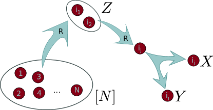
Figure 3: As an example justifying why conditional correlations cannot be erased using a noise rate equal to the CQMI without conditioning on the pivot system, consider random variables $X$, $Y$, and $Z$ constructed in the following way. $Z$ is constructed by picking a random pair of numbers $i_{1}\neq i_{2}$ from $[N]=\{1,2,...,N\}$, and $X=Y=i_{b}$ for a uniformly random bit $b$ that is independent of $Z$. Clearly $I(X:Y|Z)=1$. The classical analogue of a random unitary channel is a random permutation channel. When conditioning on $Z=(i,j)$, one can just randomize the pair $(i,j)$ using one bit of noise. Conversely, for a given pair $(i_{1},i_{2})$, the mutual information $I\left(X:Y|Z=(i_{1},i_{2})\right)$ is erased if and only if this pair is randomized by the random permutation channel. When operating on $X$ alone, this implies that all pairs have to be randomized, which essentially implies that all numbers $1,...,N$ have to be randomized jointly, requiring $\log_{2}N$ bits of noise.

The following example shows that, even for the classical analogue of state deconstruction, access to the conditioning system is necessary. Otherwise, the Markovianizing cost, as it is called in WSM15 , can be arbitrarily large compared to the conditional mutual information. The example is informally explained in Figure 3.

Let $X$ and $Y$ be random variables, each taking values from the alphabet $[n]=\{0,1,\ldots,n-1\}$, and let $Z$ be a random variable taking values in $[n]\times[n]$, such that the joint probability distribution for $(X,Y,Z)$ is as follows:

$$p_{XYZ}(i,j,(k,l))=\begin{cases}\frac{1}{n(n-1)}&\text{ if }k<l,\ i=j\in\{k,l\}\\ 0&\text{ else}\end{cases}.$$ (147)

For $k<l$, conditioned on $Z=(k,l)$, $X$ and $Y$ are maximally correlated fair coins, so that

$$I(X:Y|Z)=1.$$ (148)

One classical analogue of tracing out a subsystem is applying a function $f:[n]\to[m]$ where $n/m\in\mathbb{N}$ such that $|f^{-1}(\{j\})|=n/m$ for all $j\in[m]$.

Let $f:[n]\to[m]$ be such a function and set $X^{\prime}=f(X)$. Let $X^{\prime},Y,Z\sim p^{\prime}$ so that

$$p^{\prime}_{X^{\prime}YZ}(i,j,(k,l))=\\ \begin{cases}\frac{1}{n(n-1)}&\text{ if }k<l,\ i=f(j),j\in\{k,l\}\\ 0&\text{ else}\end{cases}.$$ (149)

Let us look at the fidelity of recovery $F(X^{\prime};Y|Z)$. It is easy to see that we can restrict to classical recovery channels: Let $\mathcal{R}_{Z\to ZX^{\prime}}$ be an arbitrary (quantum) recovery channel, denote the measurement of the computational basis on system $X$ by $\Lambda_{X}$, etc., and let $\rho_{X^{\prime}YZ}$ be the diagonal quantum state representing $p^{\prime}$. The fidelity does not decrease under the application of $\Lambda_{X^{\prime}}\otimes\Lambda_{Z}$ and any classical state is invariant, therefore $\mathcal{R}^{\prime}_{Z\to ZX^{\prime}}=(\Lambda_{X^{\prime}}\otimes\Lambda_{Z})\circ\mathcal{R}_{Z\to ZX^{\prime}}$ is at least as good a recovery channel as $\mathcal{R}_{Z\to ZX^{\prime}}$. Now as $\Lambda_{Z}(\rho_{YZ})=\rho_{YZ}$, we can also precompose a measurement without changing the fidelity; i.e., the desired classical recovery channel that is as good as $\mathcal{R}_{Z\to ZX^{\prime}}$ is $\mathcal{R}^{\prime}_{Z\to ZX^{\prime}}=(\Lambda_{X^{\prime}}\otimes\Lambda_{Z})\circ\mathcal{R}_{Z\to ZX^{\prime}}\circ\Lambda_{Z}$.

Let us then take an arbitrary classical recovery channel given by a conditional probability distribution $q_{X^{\prime}Z^{\prime}|Z}$. The resulting recovered distribution is

$$\hat{p}_{X^{\prime}YZ}(i,j,\{k,l\})$$

$$=\sum_{\begin{subarray}{c}k^{\prime}<l^{\prime}\\ k^{\prime},l^{\prime}\in[n]\end{subarray}}p_{YZ}(j,\{k^{\prime},l^{\prime}\})q_{X^{\prime}Z^{\prime}|Z}(i,\{k,l\}|\{k^{\prime},l^{\prime}\})$$ (150)

$$=\frac{1}{n(n-1)}\sum_{\begin{subarray}{c}k^{\prime}<l^{\prime}\\ k^{\prime},l^{\prime}\in[n]\end{subarray}}(\delta_{k^{\prime}j}+\delta_{l^{\prime}j})q_{X^{\prime}Z^{\prime}|Z}(i,\{k,l\}|\{k^{\prime},l^{\prime}\})$$ (151)

$$=\frac{1}{n(n-1)}\sum_{\begin{subarray}{c}l^{\prime}\in[n]\\ l^{\prime}\neq j\end{subarray}}q_{X^{\prime}Z^{\prime}|Z}(i,\{k,l\}|\{j,l^{\prime}\}).$$ (152)

Now we look at the fidelity with the original distribution, i.e.

$$\sqrt{F(p^{\prime}_{X^{\prime}YZ},\hat{p}_{X^{\prime}YZ})}$$

$$=\sum_{\begin{subarray}{c}k<l\\ k,l\in[n]\end{subarray}}\sum_{i\in[m]}\sum_{j\in[n]}\sqrt{p^{\prime}_{X^{\prime}YZ}(i,j,\{k,l\})\hat{p}_{X^{\prime}YZ}(i,j,\{k,l\})}$$ (153)

$$=\frac{1}{n(n-1)}\sum_{\begin{subarray}{c}k\neq l\\ k,l\in[n]\end{subarray}}\sqrt{\sum_{\begin{subarray}{c}l^{\prime}\in[n]\\ l^{\prime}\neq k\end{subarray}}q_{X^{\prime}Z^{\prime}|Z}(f(k),\{k,l\}|\{k,l^{\prime}\})}$$ (154)

It is obvious that the optimal recovery channel has $q_{X^{\prime}Z^{\prime}|Z}(i,\{k,l\}|\{k^{\prime},l^{\prime}\})=0$ whenever $k,l,k^{\prime},l^{\prime}$ are all different or $f(k)\neq i\neq f(l)$. Let us therefore assume this is the case. Let $\lambda_{kl}=\sum_{\begin{subarray}{c}l^{\prime}\in[n]\\ l^{\prime}\neq k\end{subarray}}q_{X^{\prime}Z^{\prime}|Z}(f(k),\{k,l\}|\{k,l^{\prime}\})$. Then we have

$$\sum_{\begin{subarray}{c}k<l\\ f(k)=f(l)\end{subarray}}\lambda_{kl}+\sum_{\begin{subarray}{c}k\neq l\\ f(k)\neq f(l)\end{subarray}}\lambda_{kl}=n(n-1)/2$$ (155)

due to the normalization of the conditional distribution $q$. Suppose first (155) and $\lambda_{kl}\geq 0$ are the only restrictions on the possible $\lambda_{kl}$. Then the optimal choice is

$$\lambda_{kl}=\frac{(n-1)}{2(n-1)-(n/m-1)},$$

i.e., constant $\lambda_{kl}$. We can now bound the fidelity of recovery

$$\sqrt{F(X^{\prime};Y|Z)_{p^{\prime}}} =\max_{q}\sqrt{F(p^{\prime},\hat{p})}$$ (156)

$$\leq\max_{\lambda_{kl}\geq 0}\frac{1}{n(n-1)}\sum_{\begin{subarray}{c}k\neq l\\ k,l\in[n]\end{subarray}}\sqrt{\lambda_{kl}}$$ (157)

$$=\sqrt{\frac{(n-1)}{2(n-1)-(n/m-1)}}.$$ (158)

Here the maxima are taken over conditional probability distributions and the positive $\lambda_{kl}$ that sum to $n(n-1)/2$, respectively. The inequality is due to the fact that by relaxing the conditions on $\lambda_{kl}$ we maximize over a larger set. For $F(X^{\prime};Y|Z)_{p^{\prime}}\geq 1-\varepsilon$ this implies

$$\log(n/m)\geq\log(n-1)+\log\left(\frac{1-2\varepsilon}{1-\varepsilon}\right)$$ (159)

In words, the required noise can be arbitrarily large compared to the conditional mutual information. A similar analysis can be done for many i.i.d. copies of $X$, $Y$, and $Z$.

References

• [1] Rolf Landauer. Irreversibility and heat generation in the computing process. IBM Journal of Research and Development, 5(3):183–191, July 1961.
• [2] John Goold, Marcus Huber, Arnau Riera, Lidia del Rio, and Paul Skrzypczyk. The role of quantum information in thermodynamics — a topical review. May 2015. arXiv:1505.07835.
• [3] Berry Groisman, Sandu Popescu, and Andreas Winter. Quantum, classical, and total amount of correlations in a quantum state. Physical Review A, 72(3):032317, September 2005. arXiv:quant-ph/0410091.
• [4] Mark M. Wilde. From classical to quantum Shannon theory. 2016. arXiv:1106.1445v7.
• [5] Jonathan Oppenheim. State redistribution as merging: introducing the coherent relay. May 2008. arXiv:0805.1065.
• [6] Anura Abeyesinghe, Igor Devetak, Patrick Hayden, and Andreas Winter. The mother of all protocols: Restructuring quantum information’s family tree. Proceedings of the Royal Society A, 465(2108):2537–2563, August 2009. arXiv:quant-ph/0606225.
• [7] Benjamin Schumacher and Michael D. Westmoreland. Approximate quantum error correction. Quantum Information Processing, 1(1/2):5–12, April 2002. arXiv:quant-ph/0112106.
• [8] Patrick Hayden, Michal Horodecki, Andreas Winter, and Jon Yard. A decoupling approach to the quantum capacity. Open Systems & Information Dynamics, 15(1):7–19, March 2008. arXiv:quant-ph/0702005.
• [9] Mario Berta, Fernando G. S. L. Brandão, Christian Majenz, and Mark M. Wilde. Conditional decoupling of quantum information. Physical Review Letters, 121(4):040504, July 2018. arXiv:1808.00135.
• [10] Patrick Hayden, Richard Jozsa, Denes Petz, and Andreas Winter. Structure of states which satisfy strong subadditivity of quantum entropy with equality. Communications in Mathematical Physics, 246(2):359–374, April 2004. arXiv:quant-ph/0304007.
• [11] Omar Fawzi and Renato Renner. Quantum conditional mutual information and approximate Markov chains. Communications in Mathematical Physics, 340(2):575–611, December 2015. arXiv:1410.0664.
• [12] Mario Berta, Kaushik Seshadreesan, and Mark M. Wilde. Rényi generalizations of the conditional quantum mutual information. Journal of Mathematical Physics, 56(2):022205, February 2015. arXiv:1403.6102.
• [13] Mark M. Wilde, Nilanjana Datta, Min-Hsiu Hsieh, and Andreas Winter. Quantum rate-distortion coding with auxiliary resources. IEEE Transactions on Information Theory, 59(10):6755–6773, October 2013. arXiv:1212.5316.
• [14] Igor Devetak and Jon Yard. Exact cost of redistributing multipartite quantum states. Physical Review Letters, 100(23):230501, June 2008.
• [15] Jon Yard and Igor Devetak. Optimal quantum source coding with quantum side information at the encoder and decoder. IEEE Transactions on Information Theory, 55(11):5339–5351, November 2009. arXiv:0706.2907.
• [16] Kaushik P. Seshadreesan and Mark M. Wilde. Fidelity of recovery, squashed entanglement, and measurement recoverability. Physical Review A, 92(4):042321, October 2015. arXiv:1410.1441.
• [17] Armin Uhlmann. The “transition probability” in the state space of a *-algebra. Reports on Mathematical Physics, 9(2):273–279, 1976.
• [18] Wojciech H. Zurek. Einselection and decoherence from an information theory perspective. Annalen der Physik, 9(11-12):855–864, November 2000. arXiv:quant-ph/0011039.
• [19] Harold Ollivier and Wojciech H. Zurek. Quantum discord: A measure of the quantumness of correlations. Physical Review Letters, 88(1):017901, December 2001. arXiv:quant-ph/0105072.
• [20] Matthias Christandl and Andreas Winter. “Squashed entanglement”: An additive entanglement measure. Journal of Mathematical Physics, 45(3):829–840, March 2004. arXiv:quant-ph/0308088.
• [21] Wojciech H. Zurek. Decoherence, einselection, and the quantum origins of the classical. Reviews of Modern Physics, 75(3):715–775, May 2003. arXiv:quant-ph/0105127.
• [22] Christopher A. Fuchs and Jeroen van de Graaf. Cryptographic distinguishability measures for quantum mechanical states. IEEE Transactions on Information Theory, 45(4):1216–1227, May 1998. arXiv:quant-ph/9712042.
• [23] Alexei Gilchrist, Nathan K. Langford, and Michael A. Nielsen. Distance measures to compare real and ideal quantum processes. Physical Review A, 71(6):062310, June 2005. arXiv:quant-ph/0408063.
• [24] Marco Tomamichel, Roger Colbeck, and Renato Renner. A fully quantum asymptotic equipartition property. IEEE Transactions on Information Theory, 55(12):5840—5847, December 2009. arXiv:0811.1221.
• [25] Elliott H. Lieb and Mary Beth Ruskai. Proof of the strong subadditivity of quantum-mechanical entropy. Journal of Mathematical Physics, 14:1938–1941, 1973.
• [26] Elliott H. Lieb and Mary Beth Ruskai. A fundamental property of quantum-mechanical entropy. Physical Review Letters, 30(10):434–436, March 1973.
• [27] Andreas Winter. Tight uniform continuity bounds for quantum entropies: conditional entropy, relative entropy distance and energy constraints. July 2015. arXiv:1507.07775.
• [28] Ming-Yong Ye, Yan-Kui Bai, and Z. D. Wang. Quantum state redistribution based on a generalized decoupling. Physical Review A, 78(3):030302, September 2008. arXiv:0805.1542.
• [29] Mario Berta, Matthias Christandl, and Dave Touchette. Smooth entropy bounds on one-shot quantum state redistribution. IEEE Transactions on Information Theory, 62(3):1425–1439, March 2016. arXiv:1409.4338.
• [30] Nilanjana Datta, Min-Hsiu Hsieh, and Jonathan Oppenheim. An upper bound on the second order asymptotic expansion for the quantum communication cost of state redistribution. September 2014. arXiv:1409.4352.
• [31] Christian Majenz, Mario Berta, Frédéric Dupuis, Renato Renner, and Matthias Christandl. Catalytic decoupling of quantum information. May 2016. arXiv:1605.00514.
• [32] Eyuri Wakakuwa, Akihito Soeda, and Mio Murao. Markovianizing cost of tripartite quantum states. April 2015. arXiv:1504.05805.
• [33] Eyuri Wakakuwa, Akihito Soeda, and Mio Murao. The cost of randomness for converting a tripartite quantum state to be approximately recoverable. December 2015. arXiv:1512.06920.
• [34] Mario Berta, Fernando G. S. L. Brandao, and Mark M. Wilde. unpublished notes, April 2015.
• [35] Masato Koashi and Nobuyuki Imoto. Operations that do not disturb partially known quantum states. Physical Review A, 66:022318, 2002.
• [36] Eyuri Wakakuwa, Akihito Soeda, and Mio Murao. A coding theorem for bipartite unitaries in distributed quantum computation. May 2015. arXiv:1505.04352.
• [37] Charles H. Bennett. Logical reversibility of computation. IBM Journal of Research and Development, 17(6):525–532, November 1973.
• [38] Andris Ambainis, Michele Mosca, Alain Tapp, and Ronald de Wolf. Private quantum channels. In 41st Annual Symposium on Foundations of Computer Science, pages 547–553, 2000. arXiv:quant-ph/0003101.
• [39] Mario Berta and Marco Tomamichel. The fidelity of recovery is multiplicative. IEEE Transactions on Information Theory, 62(4):1758–1763, April 2016. arXiv:1502.07973.
• [40] Robert Alicki and Mark Fannes. Continuity of quantum conditional information. Journal of Physics A: Mathematical and General, 37(5):L55–L57, February 2004. arXiv:quant-ph/0312081.
• [41] Kavan Modi, Aharon Brodutch, Hugo Cable, Tomasz Paterek, and Vlatko Vedral. The classical-quantum boundary for correlations: Discord and related measures. Reviews of Modern Physics, 84(4):1655–1707, November 2012. arXiv:1112.6238.
• [42] Gerardo Adesso, Thomas R. Bromley, and Marco Cianciaruso. Measures and applications of quantum correlations. May 2016. arXiv:1605.00806.
• [43] Marco Piani. Problem with geometric discord. Physical Review A, 86(3):034101, September 2012. arXiv:1206.0231.
• [44] Kaushik P. Seshadreesan, Mario Berta, and Mark M. Wilde. Rényi squashed entanglement, discord, and relative entropy differences. Journal of Physics A: Mathematical and Theoretical, 48(39):395303, September 2015. arXiv:1410.1443.
• [45] Mark M. Wilde. Multipartite quantum correlations and local recoverability. Proceedings of the Royal Society A, 471:20140941, March 2014. arXiv:1412.0333.
• [46] Vaibhav Madhok and Animesh Datta. Interpreting quantum discord through quantum state merging. Physical Review A, 83(3):032323, March 2011. arXiv:1008.4135.
• [47] Daniel Cavalcanti, Leandro Aolita, Sergio Boixo, Kavan Modi, Marco Piani, and Andreas Winter. Operational interpretations of quantum discord. Physical Review A, 83(3):032324, March 2011. arXiv:1008.3205.
• [48] Ke Li and Andreas Winter. Squashed entanglement, $k$-extendibility, quantum Markov chains, and recovery maps. October 2014. arXiv:1410.4184.
• [49] Jonathan Oppenheim. A paradigm for entanglement theory based on quantum communication. January 2008. arXiv:0801.0458.
• [50] Reinhard F. Werner. An application of Bell’s inequalities to a quantum state extension problem. Letters in Mathematical Physics, 17(4):359–363, May 1989.
• [51] Andrew C. Doherty, Pablo A. Parrilo, and Federico M. Spedalieri. Complete family of separability criteria. Physical Review A, 69(2):022308, February 2004. arXiv:quant-ph/0308032.
• [52] Fernando G. S. L. Brandao and Aram W. Harrow. Quantum de Finetti theorems under local measurements with applications. In Proceedings of the 45th ACM Symposium on Theory of Computing (STOC 2013), pages 861–870, 2013. arXiv:1210.6367.
• [53] Dawei Ding, Patrick Hayden, and Michael Walter. Conditional mutual information of bipartite unitaries and scrambling. August 2016. arXiv:1608.04750.
• [54] Dong Yang, Karol Horodecki, Michal Horodecki, Pawel Horodecki, Jonathan Oppenheim, and Wei Song. Squashed entanglement for multipartite states and entanglement measures based on the mixed convex roof. IEEE Transactions on Information Theory, 55(7):3375–3387, July 2009. arXiv:0704.2236.
• [55] David Avis, Patrick Hayden, and Ivan Savov. Distributed compression and multiparty squashed entanglement. Journal of Physics A: Mathematical and Theoretical, 41(11):115301, March 2008. arXiv:0707.2792.
• [56] Anurag Anshu, Vamsi Krishna Devabathini, and Rahul Jain. Near optimal bounds on quantum communication complexity of single-shot quantum state redistribution. October 2014. arXiv:1410.3031.
• [57] Huzihiro Araki and Elliott H. Lieb. Entropy inequalities. Communications in Mathematical Physics, 18(2):160–170, 1970.