Power corrections to the electromagnetic spectral function and the dilepton rate in QCD plasma within operator product expansion in $D=4$

Abstract

We evaluate the electromagnetic spectral function in QCD plasma in a nonperturbative background of in-medium quark and gluon condensates by incorporating the leading order power corrections in a systematic framework within the ambit of the operator product expansion in $D=4$ dimension. We explicitly show that the mixing of the composite operators removes mass singularities and renders Wilson coefficients finite and well defined. As a spectral property, we then obtain the nonperturbative dilepton production rate from QCD plasma. The operator product expansion automatically restricts the dilepton rate to the intermediate mass range, which is found to be enhanced due to the power corrections. We also compare our result with those from nonperturbative calculations, e.g., lattice QCD and effective QCD models based on Polyakov loop.

1 Introduction

Over the last couple of decades, with the international efforts from the relativistic heavy-ion collision experiments in SPS to LHC, we already have some profound signatures of the high temperature deconfined phase of quantum chromodynamics (QCD), namely quark gluon plasma (QGP). However, a locally equilibrated plasma is short-lived in the collision. However, there are always some initial or final state interactions that may contaminate an observable one is interested in. In this respect the electromagnetic emissivity of the plasma in the form of real or virtual photon is particularly important. The very fact that they do not suffer from final state interactions and carries least contaminated information of the local equilibrium makes real or virtual photon production a desirable candidate for studying QGP. Real photon escapes unperturbed and virtual photon decays into a lepton pair in the process. This is why, the photon and dilepton production rates from QGP phase have been studied vividly in the last three decades Lebellac ; Weldon:1983jn ; Weldon:1990iw ; McLerran:1984ay ; Hwa:1985xg ; Kajantie:1986dh ; Kajantie:1986cu ; Cleymans:1986na ; Cleymans:1992gb ; Gale:1987ey ; Gale:1987ki ; Braaten:1990wp ; Karsch:2000gi ; Bandyopadhyay:2015wua ; Greiner:2010zg ; Aurenche:1998nw ; Mustafa:1999dt ; Karsch:2001uw ; Ding:2010ga ; Ding:2016hua ; Islam:2014sea ; Gale:2014dfa ; Islam:2015koa ; Bandyopadhyay:2016fyd ; Sadooghi:2016jyf ; Tuchin:2013bda ; Srivastava:2002ic ; Kvasnikova:2001zm ; Chatterjee:2007xk ; Laine:2013vma ; Ghisoiu:2014mha ; Ghiglieri:2014kma .

Even though the lepton pairs behave as free particles after production, but they are produced in every stage of the collisions. The high mass dileptons are mostly produced due to collision between hard partons and not particularly very informative about QGP. This is because the Drell-Yan processes Drell:1969km and charmonium decays Dominguez:2009mk ; Dominguez:2010mx are the major processes in that regime. On the other hand the low mass dilepton production is enhanced Adare:2009qk compared to all known sources of electromagnetic decay of the hadronic particles and the contribution of a radiating QGP. So, the low mass dileptons ($\leq 1$ GeV) possibly indicates some nonhadronic sources and the intricacies are discussed in the literature in a more phenomenological way Greiner:2010zg ; Islam:2014sea ; Gale:2014dfa . There also exists dilepton production  Shuryak:1978ij in intermediate range of invariant mass (say $1-3$ GeV) with optimized contribution from the QGP, which is not dominated by hadronic processes, but still treated via perturbative methods. We emphasize that the higher order perturbative calculations Aurenche:1998nw ; Laine:2013vma ; Ghisoiu:2014mha ; Ghiglieri:2014kma of the dilepton rate do not converge in a small strong coupling ($g$) limit. This is because the temperatures attained in recent heavy-ion collisions are not so high to make perturbative calculations applicable. However, the leading order perturbative quark-antiquark annihilation is the only dilepton rate from the QGP phase that has been used extensively in the literature. Nevertheless, this contribution is very appropriate at large invariant mass but not in low and intermediate invariant mass. In this mass regime one expects that the nonperturbative contributions could be important and substantial.

The nonperturbative effects of QCD are taken care by the lattice QCD (LQCD) computations, a first principle based method of QCD. It has very reliably computed the nonperturbative effects associated with the bulk properties (thermodynamics and conserved density fluctuations) of the deconfined phase, around and above the deconfined temperature. Further, the efforts have also been made in lattice within the quenched approximation of QCD Ding:2010ga ; Ding:2016hua ; Karsch:2001uw ; Aarts:2002cc ; Kaczmarek:2011ht ; Aarts:2005hg and in full QCD Amato:2013naa ; Aarts:2014nba for studying the structure of vector correlation functions and their spectral representations. Nevertheless, such studies have provided only critically needed information about various transport coefficients both at zero Aarts:2002cc ; Kaczmarek:2011ht and finite Aarts:2005hg momentum, and the thermal dilepton rate Karsch:2001uw ; Ding:2010ga ; Ding:2016hua . The computation of these quantities proceed by first evaluating the Euclidean time correlation function only for a finite set of discrete Euclidean times to reconstruct the vector spectral function in continuous real time using maximum entropy method (MEM) Asakawa:2000tr ; Nakahara:1999vy , thereby extracting various spectral properties. Unfortunately the lattice techniques are solely applicable in Euclidean spacetime, while the spectral function is an inherently Minkowskian object. Though it can be obtained from the Euclidean correlator in principle, but the process of analytic continuation in the regime of lattice is ill-defined. Because of this complication, in LQCD the spectral function is not defined via Eq. (3) but through a probabilistic method MEM Asakawa:2000tr ; Nakahara:1999vy , which is also in some extent error prone Cuniberti:2001hm . Nevertheless, because of its limitations LQCD data Karsch:2001uw ; Ding:2010ga ; Ding:2016hua also could not shed much light on the low and intermediate mass dileptons as it is indeed a difficult task in lattice.

It is now desirable to have an alternative approach to include nonperturbative effects in dilepton production. It is well known that the QCD vacuum has a nontrivial structure consisting of non-perturbative fluctuations of the quark and gluonic fields. These fluctuations can be traced via a few phenomenological quantities, known as vacuum condensates GellMann:1968rz . In standard perturbation theory for simplicity one works with an apparent vacuum and the theory becomes less effective with relatively lower invariant mass. The vacuum expectation values of the such condensates vanishes in the perturbation theory by definition. But in reality they are non-vanishing Vainshtein:1978sz ; Lavelle:1988eg and thus the idea of the nonperturbative dynamics of QCD is signaled by the emergence of power corrections in physical observables through the inclusion of nonvanishing vacuum expectation values of local quark and gluonic operators such as the quark and gluon condensates. In present calculation we intend to compute intermediate mass (IM) dilepton production using a nonperturbative power corrections.

In this context Shifman-Vainshtein-Zakharov (SVZ) first argued Shifman:1978bx ; Shifman:1978by that Wilson’s Operator Product Expansion (OPE) Wilson:1969zs is valid in presence of the non-perturbative effects Novikov:1980uj . By using OPE judiciously one can exploit both perturbative and non-perturbative domain separately Hubschmid:1982pa ; Mallik:1983nn ; Bagan:1992tg . Unlike QED a favorable situation occurs particularly in QCD that allows us to do the power counting Novikov:1984rf ; Novikov:1984ac . OPE basically assumes a separation of large and short distance effects via condensates and Wilson coefficients. Also according to SVZ, the less effectiveness of ordinary perturbation theory at relatively low invariant mass is a manifestation of the fact that nonperturbative vacuum condensates are appearing as power corrections in the OPE of a Green’s function. So in view of OPE, in the large-momentum (short-distance) limit, a two point current-current correlation function Shifman:1978bx ; Shifman:1978by ; Narison:2002pw can be expanded in terms of local composite operators and $c$-numbered Wilson coefficients as

$$C(p) =\atop{z\rightarrow 0} i\int e^{ip\cdot z}d^{4}z\big{\langle}{\cal T}\left\{J(z)J(0)\right\}\big{\rangle}=\sum\limits_{n}W_{n}(p^{2},\nu^{2})\ \langle O_{n}\rangle_{D},$$ (1)

provided $p^{2}>>\Lambda^{2}$ , where $\Lambda$ is the QCD scale and ${\cal T}$ is the time ordered product. $O_{n}$ is the $D$-dimensional composite operators (condensates) and have non-zero expectation values which were absent to all orders in perturbation theory. $\nu$ is a factorization scale that separates long and short distance dynamics. The power corrections appear through the Wilson coefficients $W$ that contain all information about large momentum (short distance) physics above the scale $\nu$, implying that those are free from any infrared and nonperturbative long distance effects. Alternatively, the factorization scale $\nu$ is chosen to minimize the perturbative contributions to the condensates such that the physical observable should, in principle, be insensitive to the choice of $\nu$. We note that for computing a correlator in vacuum(medium) one should first calculate it in a background of quark and gluonic fields and then average it with respect to these fields in the vacuum(medium) to incorporate the power corrections through relevant condensates.

Before going into our calculation we would like note following points in OPE: The general and important issue in OPE is the separation of various scales. At finite temperature the heatbath introduces a scale $T$, and then OPE has three scales: $\Lambda$, $T$ and $p$ beside the factorization scale $\nu$. Based on this one can have either (i) $\Lambda$ and $T$ soft but $p$ hard ($\Lambda\sim T<p$) or (ii) $\Lambda$ soft but $p$ and $T$ hard ($\Lambda<p\sim T$).

1. The general belief Shuryak:1988ck ; Bochkarev:1985ex that the Wilson coefficients $W(p^{2},\nu^{2})$ are c-numbered and remain same irrespective of the states considered. This means if one takes vacuum average $\langle\cdots\rangle_{0}$ or thermal average $\langle\cdots\rangle_{\beta}$ of eq.(1), the Wilson coefficient functions, $W(p^{2},\nu^{2})$, remain temperature independent whereas the temperature dependence resides only in $\langle O\rangle_{\beta}$. In other way, OPE is an expansion in $1/p$ where $p$ is the typical momentum scale. But thermal effects are essentially down by thermal factors $\exp(-p/T)$. For $\Lambda\sim T<p$, this does not contribute to any order in $1/p$ in OPE. It is like $\exp(-1/x)$ for which all coefficients in the Taylor expansion in $x(=T/p)$ vanish.

2. There are also efforts to extend the OPE to a system with finite temperature Furnstahl:1989ji ; Hansson:1990tt ; Bochkarev:1985ex ; Bochkarev:1984zx ; Dosch:1988vt . At nonzero $T$ the heatbath introduces perturbative contributions to the matrix element in OPE, $\langle O\rangle_{\beta}$ in addition to the nonperturbative contributions of finite dimension composite operator. One needs to determine a temperature $T\sim p$ above which the perturbative calculation of thermal corrections is reliable. Usually these perturbative thermal corrections are incorporated by making the Wilson coefficients temperature dependent through systematically resummed infinite order in the expansion that comes out to be $\sim T$ (but not $\sim gT$). This means if one takes the thermal average of eq.(1), then one requires contributions to infinite order in the expansion to get $W$’s temperature dependent, and it becomes an expansion of $\Lambda/p$ whereas the expansion in $1/(p/T)$ is already resummed Furnstahl:1989ji . Nevertheless, this resummation is appropriate when $T\gtrsim p$, but QCD sum rule approach may break down and lose its predictive power Hansson:1990tt .

   However, for low temperature ($\Lambda\sim T<p$) such resummation does not make much sense. Thus for low $T$ the temperature acts as an infrared effect and cannot change the Wilson coefficients. Since our calculation is intended for low temperature ($\pi T<p<\omega$), the temperature dependence is only considered in the condensates based on the above point 1 vis-a-vis scale separtion as in case (i).

Now the in-medium differential dilepton production rate Weldon:1990iw ; McLerran:1984ay is related to the electromagnetic spectral function as

$$\frac{dR}{d^{4}xd^{4}p}=\frac{\alpha_{\textrm{e}m}}{12\pi^{3}M^{2}}n_{B}\left(\omega\right)\sum\limits_{f}q_{f}^{2}\,\rho_{f}(\omega,|\vec{p}|),$$ (2)

where $n_{B}(x)=(e^{x}-1)^{-1}$ is the Bose-Einstein distribution function, $q_{f}$ is the electric charge of a given quark flavor $f$, $\alpha_{\textrm{e}m}$ is the electromagnetic fine structure constant and the invariant mass of the lepton pair is $M^{2}=p^{2}=\omega^{2}-|\vec{p}|^{2}$ with $p\equiv(\omega,\vec{p})$. The dilepton rate in (2) is valid only at leading order in $\alpha_{\textrm{e}m}$ but to all orders in strong coupling constant $\alpha_{s}$. The quark and lepton masses are neglected in (2).

The electromagnetic spectral function for a given flavor $f$, $\rho_{f}\left(\omega,|\vec{p}|\right)$, is extracted from the timelike discontinuity of the two point correlation function as

$$\rho_{f}\left(\omega,|\vec{p}|\right)=\frac{1}{\pi}\,\mathrm{Im}\left(C^{\mu}_{\mu}\right)_{f}.$$ (3)

The main aim of the present paper is to obtain the in-medium electromagnetic spectral function incorporating the power corrections within OPE in $D=4$ dimension and analyze its effect on the thermal dilepton rate from QGP. To obtain the in-medium electromagnetic spectral function one needs to calculate the two point correlation function via OPE corresponding to the $D=4$ gluonic and quark operators (condensates) in hot QCD medium. The power corrections appears in the spectral function through the nonanalytic behavior of the correlation function in powers of $p^{-D/2}$ or logarithms in the Wilson coefficients within OPE in $D$ dimension.

The plan of the paper is as follows. In section 2 we outline some generalities needed for the purpose. In sections 3 and 4 we discuss how in-medium quark and gluonic composite operators in $D=4$, respectively, can be included in electromagnetic polarization diagram. We then obtain the two point correlators in terms of Wilson coefficients and those composite operators for the case of light quarks. We also demonstrate how the mass singularity appearing in the correlator is absorbed by using minimal subtraction via operator mixing. In section 5 we discuss about the thermal spectral function and it’s modification due to incorporation of leading order power correction, particularly in the range of intermediate invariant mass. As a spectral property the dilepton production is discussed in section 6 and compare our results with some other known perturbative and nonperturbative results and then we conclude in section 7.

2 Setup

We briefly outline some generalities which are essential ingredients in our calculation. In usual notation the nonabelian field tensor in $SU(3)$ is defined as

$$G_{\mu\nu}^{a} = \partial_{\mu}A_{\nu}^{a}-\partial_{\nu}A_{\mu}^{a}+gf^{abc}A_{\mu}^{b}A_{\nu}^{c},$$

$$G_{\mu\nu} = G_{\mu\nu}^{a}t^{a},$$

$$D_{\alpha} = \partial_{\alpha}-igt^{a}A_{\mu}^{a},\$$ (4)

where $a,b,c$ are color indices, $t^{a}$ are the generators and $g_{\mu\nu}=\text{diag}(1,-1,-1,-1)$. Consequently in vacuum it satisfies the projection relation for composite operator

$$\Big{\langle}G_{\mu\nu}^{a}(0)G_{\alpha\beta}^{b}(0)\Big{\rangle} = \frac{1}{96}\delta^{ab}(g_{\mu\alpha}g_{\nu\beta}-g_{\mu\beta}g_{\nu\alpha})\Big{\langle}G_{\rho\sigma}^{c}G^{c~{}\rho\sigma}\Big{\rangle}.$$ (5)

Choosing the Fock-Schwinger aka the fixed point gauge ($x^{\mu}A_{\mu}^{a}(x)=0$) for convenience, the gauge field $A_{\mu}^{a}(x)$ can be expressed easily in terms of gauge covariant quantities Smilga:1982wx ; Reinders:1984sr ; Novikov:1984rf ; Novikov:1984ac as

$$A_{\mu}(x)=\int\limits_{0}^{1}\sigma~{}d\sigma~{}G_{\nu\mu}(\sigma x)x^{\nu}=\frac{1}{2}x^{\nu}G_{\nu\mu}(0)+\frac{1}{3}x^{\alpha}x^{\nu}D_{\alpha}G_{\nu\mu}(0)+\cdots\,,$$

where first the gauge field $G(y)$ has been Taylor expanded in the small $\sigma$ limit and then the integration over $\sigma$ has been performed. Now in momentum space it reads

$$A_{\mu}(k) = \int A_{\mu}(x)e^{ikx}d^{4}x$$ (6)

$$= \frac{-i(2\pi)^{4}}{2}G_{\nu\mu}(0)\frac{\partial}{\partial k_{\nu}}\delta^{4}(k)+\frac{(-i)^{2}(2\pi)^{4}}{2}(D_{\alpha}G_{\nu\mu}(0))\frac{\partial^{2}}{\partial k_{\nu}\partial k_{\alpha}}\delta^{4}(k)+\cdots,$$

where each background gluon line will be associated with a momentum integration as we will see below. Using this one can now evaluate the effective quark propagator in presence of background gluon lines Novikov:1984rf ; Novikov:1984ac by expanding the number of gluon legs attached to the bare quark line as in Fig. 1. So, it can be written as

$$S_{\textrm{eff}} = S_{0}+S_{1}+S_{2}+\cdots,$$ (7)

where the bare propagator for massive quark reads as

$$S_{0} = \frac{i}{\not{k}-m}$$ (8)

where $m$ is the mass of the quark.

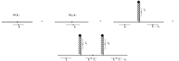
Figure 1: Effective quark propagator in the background gluon field.

With one gluon leg attached to the bare quark (Fig. 1) the expression reads as

$$S_{1} = \frac{-i}{\not{k}-m}\int\frac{d^{4}l_{1}}{(2\pi)^{4}}\frac{\not{A}(l_{1})}{\not{k}-\not{l_{1}}-m}$$ (9)

$$= -\frac{i}{4}gt^{a}G_{\mu\nu}^{a}(0)\frac{1}{(k^{2}-m^{2})^{2}}\{\sigma^{\mu\nu}(\not{k}+m)+(\not{k}+m)\sigma^{\mu\nu}\},$$

where

$$\sigma^{\mu\nu} = \frac{i}{2}[\gamma^{\mu},\gamma^{\nu}],$$

and the background gauge field $\not{A}(l_{1})$ is replaced by the first term of the gauge field as given in Eq. (6). Similarly for the diagram where two gluon legs are attached to the bare quark, we get

$$S_{2} = \frac{i}{\not{k}-m}\int\frac{d^{4}l_{1}}{(2\pi)^{4}}\frac{\not{A}(l_{1})}{\not{k}-\not{l_{1}}-m}\int\frac{d^{4}l_{2}}{(2\pi)^{4}}\frac{\not{A}(l_{2})}{\not{k}-\not{l_{1}}-\not{l_{2}}-m}$$ (10)

$$= -\frac{i}{4}g^{2}t^{a}t^{b}G_{\alpha\beta}^{a}(0)G_{\mu\nu}^{b}(0)\frac{(\not{k}+m)}{(k^{2}-m^{2})^{5}}(f^{\alpha\beta\mu\nu}+f^{\alpha\mu\beta\nu}+f^{\alpha\mu\nu\beta}),$$

where

$$f^{\alpha\beta\mu\nu} = \gamma^{\alpha}(\not{k}+m)\gamma^{\beta}(\not{k}+m)\gamma^{\mu}(\not{k}+m)\gamma^{\nu}(\not{k}+m).$$

In presence of a medium, however, a four-vector $u_{\mu}=(1,0,0,0)$ is usually introduced to restore Lorentz invariance in the rest frame of the heat bath. So, at finite temperature additional scalar operators can be constructed so that the vacuum operators are generalized to in-medium ones. The projection relation of composite operator in (5) gets modified in finite temperature Mallik:1997pq ; Mallik:1983nn ; Antonov:2004mt ; Basar:2014swa as

$$\big{\langle}G_{\mu\nu}^{a}(0)G_{\alpha\beta}^{b}(0)\big{\rangle}_{T} = \big{[}g_{\mu\alpha}g_{\nu\beta}-g_{\mu\beta}g_{\nu\alpha}\big{]}A-\big{[}(u_{\mu}u_{\alpha}g_{\nu\beta}-u_{\mu}u_{\beta}g_{\nu\alpha}-u_{\nu}u_{\alpha}g_{\mu\beta}$$ (11)

$$+u_{\nu}u_{\beta}g_{\mu\alpha})-\frac{1}{2}(g_{\mu\alpha}g_{\nu\beta}-g_{\mu\beta}g_{\nu\alpha})\big{]}B+i\epsilon_{\mu\nu\alpha\beta}C,$$

where $A,B\,\textrm{and}\,C$ are, respectively, given as

$$A=\frac{\delta^{ab}}{96}\big{\langle}G^{2}\big{\rangle}_{T},~{}B=\frac{\delta^{ab}}{12}\big{\langle}u\Theta^{g}u\big{\rangle}_{T},~{}C=\frac{\delta^{ab}}{96}\big{\langle}{\cal E}\cdot{\cal B}\big{\rangle}_{T}$$

with ${\cal E}$ and ${\cal B}$ are, respectively, the electric and magnetic fileds. The traceless gluonic stress tensor, $\Theta^{g}_{\mu\nu}$, is given by

$$\Theta^{g}_{\mu\nu}=-G_{\mu\rho}^{a}G_{\nu}^{a\rho}+\frac{1}{4}g_{\mu\nu}G^{a}_{\rho\sigma}G^{\rho\sigma~{}a}.$$ (12)

QCD vacuum consists of both quark and gluonic fields. We note that the composite operators involving quark fields will be defined below whenever necessary.

3 Composite Quark Operators

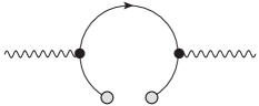
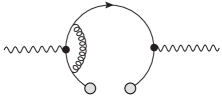
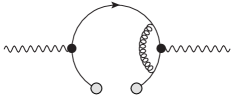
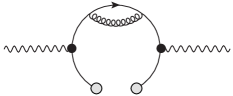
Figure 2: OPE topologies corresponding to $D=4$ composite quark operator that can contribute to the power correction in the one-loop electromagnetic polarization. The composite quark operator is denoted by two gray blobs separated by a gap in the internal quark line. Top left one contributes to the leading order (LO:$e^{2}$) whereas the remaining three are due to gluonic corrections contribute to non-leading order (NLO: $e^{2}g^{2}$).

In this section we would like to discuss the power corrections using composite quark operators (condensates) in OPE. In presence of quark condensate the leading order contribution comes from the top left panel in Fig. 2 where one of the internal quark line is soft in the polarization diagram represented by two gray blobs with a gap. We note that the diagrams here are not thermal field theory diagrams but$``$OPE diagrams” with scales: $\Lambda$ and $T$ soft but $p$ hard ($\Lambda\sim T<p$). The corresponding contributions can be obtained as

$$\Big{[}C^{\textrm{LO}}_{\mu\nu}(p)\Big{]}_{q} = i\int e^{ip\cdot z}d^{4}z\big{\langle}{\cal T}\{j_{\mu}(z)j_{\mu}(0)\}\big{\rangle}$$ (13)

$$= -N_{c}N_{f}\int e^{ip\cdot z}d^{4}z\textrm{Tr}\big{[}\bar{\psi}(z)\gamma_{\mu}S(z,0)\gamma_{\nu}\psi(0)+\bar{\psi}(0)\gamma_{\nu}S(0,z)\gamma_{\mu}\psi(z)\big{]},$$

where $N_{f}$ is the number of quark flavor and $N_{c}$ is the number of color for a given flavor. We also note that the soft quark lines are represented by Heisenberg operators $\psi(z)$ and $\psi(0)$. In the large $p$ limit, $\psi(z)$ can be expanded as

$$\psi(z)=\psi(0)+z^{\mu}D_{\mu}\psi(0).$$ (14)

Now considering only the first term in the expansion of (14) in (13), one gets

$$\Big{[}C^{\textrm{LO}}_{\mu\nu}(p)\Big{]}^{1}_{q} = -N_{c}N_{f}\frac{1}{12}\big{\langle}\bar{\psi}\psi\big{\rangle}\textrm{Tr}\big{[}\gamma_{\mu}S(p)\gamma_{\nu}+\gamma_{\nu}S(p)\gamma_{\mu}\big{]},$$ (15)

which, as expected, vanishes in the chiral limit. This is because of the appearance of the chiral condensate, $\langle\bar{\psi}\psi\rangle$ which is proportional to the quark mass $m$. On the other hand, choosing the second term in the expansion of (14) we get

$$\Big{[}C^{\textrm{LO}}_{\mu\nu}(p)\Big{]}^{2}_{q}\!\! = \!\!-N_{c}N_{f}\!\!\int e^{ip\cdot z}\,\,d^{4}z\,\,\times$$ (16)

$$\textrm{Tr}\left[\bar{\psi}(0)z^{\rho}\overleftarrow{D}_{\rho}\gamma_{\mu}S(z,0)\gamma_{\nu}\psi(0)+\bar{\psi}(0)\gamma_{\nu}S(0,z)\gamma_{\mu}z^{\rho}\overrightarrow{D}_{\rho}\psi(0)\right].$$

Now the most general decomposition of $\langle\bar{\psi}iD_{\rho}\psi\rangle$ for the massless at finite temperature Mallik:1997pq is given as

$$\langle\bar{\psi}iD_{\rho}\psi\rangle_{T} = \left(-\frac{1}{12}\gamma_{\rho}+\frac{1}{3}u_{\rho}\not{u}\right)\langle u\Theta^{f}u\rangle_{T},$$ (17)

where $\Theta^{f}_{\mu\nu}$ is traceless fermionic stress tensor and in the massless limit it is given by

$$\Theta^{f}_{\mu\nu}=\bar{\psi}\gamma_{\mu}iD_{\nu}\psi.$$ (18)

Using (17) in (16), and performing $z$-integration one gets

$$\Big{[}C^{\textrm{LO}}_{\mu\nu}(p)\Big{]}^{2}_{q} = -N_{c}N_{f}~{}\frac{\partial}{\partial p^{\rho}}\textrm{Tr}\Big{[}\big{(}\gamma_{\mu}S(p)\gamma_{\nu}+\gamma_{\nu}S(p)\gamma_{\mu}\big{)}\big{(}-\gamma_{\rho}+4u_{\rho}\not{u}\big{)}\Big{]}\frac{1}{12}\big{\langle}u\Theta^{f}u\big{\rangle}_{T}.$$ (19)

Now treating the Wilson coefficients temperature independent, the LO contribution is obtained as

$$\Big{[}C^{\mu\,\textrm{LO}}_{\mu}(p)\Big{]}_{q} = \Big{[}C^{\mu\,\textrm{LO}}_{\mu}(p)\Big{]}^{2}_{Q}=\frac{8N_{c}N_{f}}{3p^{2}}\left(1-4\frac{\omega^{2}}{p^{2}}\right)\big{\langle}u\Theta^{f}u\big{\rangle}_{T}.$$ (20)

We note that the contributions from NLO order gluonic corrections (Fig. 2) to quark vacuum condensates are already evaluated in Pascual:1981jr . Following the same prescription as LO the total NLO in-medium contributions from remaining three diagrams in Fig.2 in the massless limit is obtained as

$$\Big{[}C^{\mu\,\textrm{NLO}}_{\mu}(p)\Big{]}_{q} = \frac{8N_{c}N_{f}}{3p^{2}}\big{\langle}u\Theta^{f}u\big{\rangle}_{T}\left(1-4\frac{\omega^{2}}{p^{2}}\right)\frac{2g^{2}}{9\pi^{2}}\left(1-\ln\left(\frac{-p^{2}}{\Lambda^{2}}\right)\right).$$ (21)

We note that the logarithmic correction appears from the radiative correction diagrams in Fig.2 when the ultraviolet divergences associated with them are regularized through dimensional regularization peskin . The non-analytic behaviour of this logarithmic term will generate the power tail in the spectral function.

Combining (20) and (21) one obtains power correction upto NLO due to quark operator in the electromagnetic correlation function at finite temperature as

$$\Big{[}C_{\mu}^{\mu}(p)\Big{]}_{q} = \frac{8N_{c}N_{f}}{3p^{2}}\big{\langle}u\Theta^{f}u\big{\rangle}_{T}\left(1-4\frac{\omega^{2}}{p^{2}}\right)\left[1+\frac{2g^{2}}{9\pi^{2}}\left(1-\ln\left(\frac{-p^{2}}{\Lambda^{2}}\right)\right)\right].$$ (22)

4 Composite Gluonic Operators

In this section we compute the power correction to the electromagnetic correlation function from the $D=4$ composite gluonic operator by considering the soft gluon lines attached to the internal quark lines in the electromagnetic polarization diagram. There are two such topologies, as shown in Figs. 3 and 4, depending upon how the soft gluon line is attached to the internal quark lines in electromagnetic polarization diagram.

Using Eqs.(8)-(10), the contribution of the vertex correction diagram (topology-I) in vacuum can be written as

$$\Big{[}C_{\mu}^{\mu}(p)\Big{]}_{g}^{\textrm{I}} = iN_{c}N_{f}\int\frac{d^{4}k}{(2\pi)^{4}}\textrm{Tr}\Big{[}\gamma_{\mu}S_{1}(k)\gamma^{\mu}S_{1}(q)\Big{]}$$ (23)

$$= -\frac{iN_{c}N_{f}}{16}g^{2}t^{a}t^{b}\Big{\langle}G_{\rho\sigma}^{a}(0)G_{\alpha\beta}^{b}(0)\Big{\rangle}$$

$$\times\int\frac{d^{4}k}{(2\pi)^{4}}\frac{\textrm{Tr}\Big{[}\gamma_{\mu}\left(\sigma^{\rho\sigma}(\not{k}+m)+(\not{k}+m)\sigma^{\rho\sigma}\right)\gamma^{\mu}\left(\sigma^{\alpha\beta}(\not{q}+m)+(\not{q}+m)\sigma^{\alpha\beta}\right)\Big{]}}{(k^{2}-m^{2})^{2}(q^{2}-m^{2})^{2}}$$

$$= -iN_{c}N_{f}\Big{\langle}g^{2}G^{2}\Big{\rangle}\int\frac{d^{4}k}{(2\pi)^{4}}\frac{k\cdot q}{(k^{2}-m^{2})^{2}(q^{2}-m^{2})^{2}},$$

where $q=k-p$ and we have also used Eq.(5) in the last step after evaluating the trace.

Similarly, the contribution from the topology-II (including the one where two gluon lines are attached to the other quark propagator in Fig.4) in vacuum can be written as

$$\Big{[}C_{\mu}^{\mu}(p)\Big{]}_{g}^{\textrm{II}} = 2iN_{c}N_{f}\int\frac{d^{4}k}{(2\pi)^{4}}\textrm{Tr}\Big{[}\gamma_{\mu}S_{2}(k)\gamma^{\mu}S_{0}(q)\Big{]}$$ (24)

$$= \frac{iN_{c}N_{f}}{4}g^{2}t^{a}t^{b}\Big{\langle}G_{\rho\sigma}^{a}(0)G_{\alpha\beta}^{b}(0)\Big{\rangle}$$

$$\times\int\frac{d^{4}k}{(2\pi)^{4}}\frac{\textrm{Tr}\Big{[}\gamma_{\mu}(\not{k}+m)(f^{\alpha\beta\mu\nu}+f^{\alpha\mu\beta\nu}+f^{\alpha\mu\nu\beta})\gamma^{\mu}\left(\not{q}+m\right)\Big{]}}{(k^{2}-m^{2})^{5}(q^{2}-m^{2})}$$

$$= -iN_{c}N_{f}\Big{\langle}g^{2}G^{2}\Big{\rangle}\int\frac{d^{4}k}{(2\pi)^{4}}\frac{4m^{2}(k\cdot q-2k^{2})}{(k^{2}-m^{2})^{4}(q^{2}-m^{2})}.$$

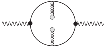
Figure 3: (Topology-I) Vertex correction where one soft gluon line is attached to each internal quark line in the electromagnetic polarization diagram.

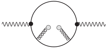
Figure 4: (Topology-II) Self-energy correction where two soft gluon lines are attached to one internal quark line in the electromagnetic polarization diagram. A similar topology will also arise when two soft gluon lines are attached to the other quark line.

Now, we would like to compute both topologies in presence of $D=4$ composite gluonic operators at finite $T$. For the purpose, unlike vacuum case one requires to use in-medium gluon condensates as given in Eq.(11). The vacuum contributions in Eqs.(23) and (24) are, respectively, modified at finite $T$ as

$$\Big{[}C_{\mu}^{\mu}(p)\Big{]}_{g,T}^{\textrm{I}} = -\frac{iN_{c}N_{f}}{16}g^{2}t^{a}t^{b}\Big{\langle}G_{\rho\sigma}^{a}(0)G_{\alpha\beta}^{b}(0)\Big{\rangle}_{T}$$ (25)

$$\times\int\frac{d^{4}k}{(2\pi)^{4}}\frac{\textrm{Tr}\Big{[}\gamma_{\mu}\big{(}\sigma^{\rho\sigma}(\not{k}+m)+(\not{k}+m)\sigma^{\rho\sigma}\big{)}\gamma^{\mu}\big{(}\sigma^{\alpha\beta}(\not{q}+m)+(\not{q}+m)\sigma^{\alpha\beta}\big{)}\Big{]}}{(k^{2}-m^{2})^{2}(q^{2}-m^{2})^{2}}$$

$$= -iN_{c}N_{f}\Big{\langle}g^{2}G^{2}\Big{\rangle}_{T}\int\frac{d^{4}k}{(2\pi)^{4}}\frac{k\cdot q}{(k^{2}-m^{2})^{2}(q^{2}-m^{2})^{2}}$$

$$+\frac{4iN_{c}N_{f}}{3}\Big{\langle}g^{2}u\Theta^{g}u\Big{\rangle}_{T}\int\frac{d^{4}k}{(2\pi)^{4}}\frac{(k\cdot q-4k_{0}q_{0})}{(k^{2}-m^{2})^{2}(q^{2}-m^{2})^{2}},$$

and

$$\Big{[}C_{\mu}^{\mu}(p)\Big{]}_{g,T}^{\textrm{II}} = \frac{iN_{c}N_{f}}{4}g^{2}t^{a}t^{b}\Big{\langle}G_{\rho\sigma}^{a}(0)G_{\alpha\beta}^{b}(0)\Big{\rangle}_{T}$$

$$\times\int\frac{d^{4}k}{(2\pi)^{4}}\frac{\textrm{Tr}\Big{[}\gamma_{\mu}(\not{k}+m)(f^{\alpha\beta\mu\nu}+f^{\alpha\mu\beta\nu}+f^{\alpha\mu\nu\beta})\gamma^{\mu}\left(\not{q}+m\right)\Big{]}}{(k^{2}-m^{2})^{5}(q^{2}-m^{2})}$$

$$= -4iN_{c}N_{f}m^{2}\Big{\langle}g^{2}G^{2}\Big{\rangle}_{T}\int\frac{d^{4}k}{(2\pi)^{4}}\frac{(k\cdot q-2k^{2})}{(k^{2}-m^{2})^{4}(q^{2}-m^{2})}+\frac{32iN_{c}N_{f}}{3}\Big{\langle}g^{2}u\Theta^{g}u\Big{\rangle}_{T}$$ (26)

$$\times\int\frac{d^{4}k}{(2\pi)^{4}}\frac{k\cdot q(2k_{0}^{2}-\frac{1}{2}m^{2})+m^{2}(k^{2}-4k_{0}^{2})-2k_{0}q_{0}(k^{2}-m^{2})}{(k^{2}-m^{2})^{4}(q^{2}-m^{2})}.$$

Now, in the short-distance or large-momentum limit of nonperturbative power correction, one can work with massless quarks without loss of generality. In the massless limit Eq.(25) reduces to

$$\Big{[}C_{\mu}^{\mu}(p)\Big{]}_{g,T}^{\textrm{I}} =\atop{m\rightarrow 0} -iN_{c}N_{f}\Big{\langle}g^{2}G^{2}\Big{\rangle}_{T}\int\frac{d^{4}k}{(2\pi)^{4}}\frac{k\cdot q}{(k^{2})^{2}(q^{2})^{2}}$$ (27)

$$+\frac{4iN_{c}N_{f}}{3}\Big{\langle}g^{2}u\Theta^{g}u\Big{\rangle}_{T}\int\frac{d^{4}k}{(2\pi)^{4}}\frac{(k\cdot q-4k_{0}q_{0})}{(k^{2})^{2}(q^{2})^{2}},$$

whereas for Eq.(26) the coefficient for $\langle g^{2}G^{2}\rangle_{T}$ vanishes and it takes a simple form

$$\Big{[}C_{\mu}^{\mu}(p)\Big{]}_{g,T}^{\textrm{II}} =\atop{m\rightarrow 0} \frac{32iN_{c}N_{f}}{3}\Big{\langle}g^{2}u\Theta^{g}u\Big{\rangle}_{T}\int\frac{d^{4}k}{(2\pi)^{4}}\frac{2(k\cdot qk_{0}^{2}-k_{0}q_{0}k^{2})}{(k^{2})^{4}(q^{2})}.$$ (28)

Here we emphasize the fact that the vacuum correlation function corresponding to topology-II (self-energy correction) in Eq.(24) vanishes in the massless limit. But in medium, one obtains a finite contribution in the massless limit as found in Eq.(28) due to the in-medium condensates. Now, the integrals in the above expressions can be expressed in terms of standard Feynman integrals $\mathcal{I}_{mn}$, $\mathcal{I}_{mn}^{\mu}$ and $\mathcal{I}_{mn}^{\mu\nu}$ which have been evaluated in appendix A.1. Using those results in appendix A.1, Eqs.(27) and (28) in the massless limit ($p_{0}=\omega$), respectively, become

$$\Big{[}C_{\mu}^{\mu}(p)\Big{]}_{g,T}^{\textrm{I}} =\atop{m\rightarrow 0} -iN_{c}N_{f}\langle g^{2}G^{2}\rangle_{T}~{}\frac{1}{2}(2\mathcal{I}_{12}-p^{2}\mathcal{I}_{22})$$ (29)

$$+\frac{4iN_{c}N_{f}}{3}\langle g^{2}u\Theta^{g}u\rangle_{T}~{}\frac{1}{2}(2\mathcal{I}_{12}-p^{2}\mathcal{I}_{22}+8p_{0}\mathcal{I}_{22}^{0}-8\mathcal{I}_{22}^{00})$$

$$= \langle G^{2}\rangle_{T}~{}\frac{g^{2}N_{c}N_{f}}{16\pi^{2}p^{2}}-\langle u\Theta^{g}u\rangle_{T}~{}\frac{g^{2}N_{c}N_{f}}{3\pi^{2}p^{2}}\left[\frac{\omega^{2}}{p^{2}}-\frac{1}{4}\right],$$

and

$$\Big{[}C_{\mu}^{\mu}(p)\Big{]}_{g,T}^{\textrm{II}} =\atop{m\rightarrow 0} \frac{32iN_{c}N_{f}}{3}\langle g^{2}u\Theta^{g}u\rangle_{T}~{}(2p_{0}\mathcal{I}_{31}^{0}-\mathcal{I}_{31}^{00}-p^{2}\mathcal{I}_{41}^{00})$$ (30)

$$= -\frac{g^{2}N_{c}N_{f}}{9\pi^{2}p^{2}}\langle u\Theta^{g}u\rangle_{T}~{}\left[\frac{1}{\tilde{\epsilon}}\left(1-\frac{4\omega^{2}}{p^{2}}\right)+2-6\frac{\omega^{2}}{p^{2}}\right].$$

We note that Eq.(30) has a mass singularity as ${1}/{\tilde{\epsilon}}={1}/{\epsilon}-\ln\left({-p^{2}}/{\Lambda^{2}}\right)$ and the reason for which could be understood in the following way: while computing the self-energy correction corresponding to topology-II in Fig. 4, one actually overcounts a contribution from quark condensate. This is because the quark line in-between two soft gluon lines in Fig. 4 becomes soft, leading to quark condensate. So the actual contribution from the gluonic operators can only be obtained after minimally subtracting the quark condensate contribution Generalis:1983hb ; Broadhurst:1984rr which should cancel the mass singularity arising in the massless limitNikolaev:1982rq ; Nikolaev:1982ra ; Nikolaev:1981ff .

To demonstrate this we begin by considering finite quark mass in which a correlator containing quark condensates ($\mathcal{Q}_{k}$) can be expressed via gluon condensates ($\mathcal{G}_{n}$) Grozin:1994hd in mixed representation as

$$\mathcal{Q}_{k}=\sum_{n}c_{kn}(m)\mathcal{G}_{n},$$ (31)

where, $c_{kn}(m)$ is an expansion in $1/m$. Then one can also represent a correlator with gluon condensates ($\mathcal{G}_{n}$) as

$$\Big{[}C_{\mu}^{\mu}(p)\Big{]}_{g} = \sum_{n}a_{n}(p^{2},m)\mathcal{G}_{n},$$ (32)

whereas for quark condensates ($\mathcal{Q}_{k}$) it can be written as

$$\Big{[}C_{\mu}^{\mu}(p)\Big{]}_{q} = \sum_{k}b_{k}(p^{2},m)\mathcal{Q}_{k},$$ (33)

with $a_{n}$ and $b_{k}$ are the corresponding coefficients for the gluon and quark condensates, respectively. Now, in general a correlator with minimal subtraction using Eqs. (31), (32) and (33) can now be written as

$$\Big{[}C_{\mu}^{\mu}(p)\Big{]}_{g}^{\textrm{a}} = \Big{[}C_{\mu}^{\mu}(p)\Big{]}_{g}-\Big{[}C_{\mu}^{\mu}(p)\Big{]}_{q}=\sum_{n}a_{n}(p^{2},m)\mathcal{G}_{n}-\sum_{n,k}b_{k}(p^{2},m)c_{kn}(m)\mathcal{G}_{n}.$$ (34)

We note here that after this minimal subtraction with massive correlators and then taking the massless limit renders the resulting correlator finite. Since we are working in a massless limit, one requires an appropriate modification Broadhurst:1984rr ; Broadhurst:1985js of Eq.(31). The difference between a renormalized quark condensate and a bare one can be written as Grozin:1994hd ,

$$\mathcal{Q}_{k}-\mathcal{Q}_{k}^{b}=-\frac{1}{\epsilon}\sum_{d_{n}\leq d_{k}}m^{d_{k}-d_{n}}\gamma_{kn}\mathcal{G}_{n},$$ (35)

where $d_{n}$ and $d_{k}$ represents the dimensions of $\mathcal{G}_{n}$ and $\mathcal{Q}_{k}$ and $\gamma_{kn}$ are the mixing coefficients of $\mathcal{Q}_{k}$ with $\mathcal{G}_{n}$. Now if one wants to go to $m\rightarrow 0$ limit, $\mathcal{Q}_{k}^{b}$ vanishes because there is no scale involved in it. Also only $d_{n}=d_{k}$ term survives producing

$$\mathcal{Q}_{k}=-\frac{1}{\epsilon}\sum_{d_{n}=d_{k}}\gamma_{kn}\mathcal{G}_{n}.$$ (36)

Using Eq. (36) in the first line of Eq.(34) one can write

$$\Big{[}C_{\mu}^{\mu}(p)\Big{]}_{g}^{\textrm{a}}=\Big{[}C_{\mu}^{\mu}(p)\Big{]}_{g}+\frac{1}{\epsilon}\sum\limits_{d_{n}=d_{k}}b_{k}(p)\gamma_{kn}\mathcal{G}_{n},$$ (37)

where, $b_{k}(p)$ is the coefficient of the quark condensate $\mathcal{Q}_{k}$ in the massless limit, which is of similar dimension as $\mathcal{G}_{n}$.

So, for minimal subtraction of the quark condensate contribution overestimated in Eq.(30), the in-medium quark condensate (appearing in Eq.(22)) has to be expressed in terms of the in-medium gluon condensates of the same dimension as Zschocke:2011aa

$$\big{\langle}\bar{\psi}\gamma_{\mu}iD_{\nu}\psi\big{\rangle}_{T} = \big{\langle}:\bar{\psi}\gamma_{\mu}iD_{\nu}\psi:\big{\rangle}_{T}+\frac{3}{16\pi^{2}}m^{4}g_{\mu\nu}\left(\ln\frac{\mu^{2}}{m^{2}}+1\right)-\frac{g_{\mu\nu}}{48}\Big{\langle}\frac{g^{2}}{4\pi^{2}}G^{2}\Big{\rangle}_{T}$$ (38)

$$-\frac{1}{18}(g_{\mu\nu}-4u_{\mu}u_{\nu})\left(\ln\frac{\mu^{2}}{m^{2}}-\frac{1}{3}\right)\Big{\langle}\frac{g^{2}}{4\pi^{2}}u\Theta^{g}u\Big{\rangle}_{T},$$

where the first term in the right hand side represents the normal ordered condensate. After contracting Eq.(38) by $u^{\mu}u^{\nu}$ and applying Eq.(18) we obtain,

$$\langle u\Theta^{f}u\rangle = \textrm{Other nonrelevant terms~{}}+\frac{1}{6}\left(\ln\frac{\mu^{2}}{m^{2}}-\frac{1}{3}\right)\Big{\langle}\frac{g^{2}}{4\pi^{2}}u\Theta^{g}u\Big{\rangle}.$$ (39)

Now comparing Eqs.(39) and (36) we find

$$\gamma_{kn}=\frac{1}{6},~{}~{}b_{k}(p)=\frac{8N_{c}N_{f}}{3p^{2}}\left(1-\frac{4\omega^{2}}{p^{2}}\right).$$ (40)

Therefore, the electromagnetic correlator with gluon condensates for self-energy correction (topology-II) in the massless limit can now be written as

$$\Big{[}C_{\mu}^{\mu}(p)\Big{]}_{g,T}^{\textrm{II,a}} =\atop{m\rightarrow 0} \Big{[}C_{\mu}^{\mu}(p)\Big{]}_{g,T}^{\textrm{II}}+\frac{1}{\epsilon}\sum\limits_{d_{n}=d_{k}}b_{k}(p)\gamma_{kn}\mathcal{G}_{n},$$ (41)

$$= -\frac{g^{2}N_{c}N_{f}}{9\pi^{2}p^{2}}\langle u\Theta^{g}u\rangle_{T}\left[\frac{1}{\tilde{\epsilon}}\left(1-\frac{4\omega^{2}}{p^{2}}\right)+2-6\frac{\omega^{2}}{p^{2}}\right]+\frac{1}{\epsilon}\frac{g^{2}N_{c}N_{f}}{9\pi^{2}p^{2}}\left(1-4\frac{\omega^{2}}{p^{2}}\right)\langle u\Theta^{g}u\rangle_{T}$$

$$= -\frac{g^{2}N_{c}N_{f}}{9\pi^{2}p^{2}}\langle u\Theta^{g}u\rangle_{T}\left[-\ln\left(\frac{-p^{2}}{\Lambda^{2}}\right)\left(1-\frac{4\omega^{2}}{p^{2}}\right)+2-6\frac{\omega^{2}}{p^{2}}\right].$$

So, the minimal subtraction eventually cancels the divergence from the expression of gluonic operators. Now combining Eq.(29) and Eq.(41), the final expression for the gluonic contribution in the self-energy power correction is given by,

$$\Big{[}C_{\mu}^{\mu}(p)\Big{]}_{g,T}\!\!\!\!\!\!\!\!=\frac{g^{2}N_{c}N_{f}}{\pi^{2}p^{2}}\left[\frac{1}{9}\big{\langle}u\Theta^{g}u\big{\rangle}_{T}\left(\ln\left(\frac{-p^{2}}{\Lambda^{2}}\right)\!\left(1-\frac{4\omega^{2}}{p^{2}}\right)+9\frac{\omega^{2}}{p^{2}}-\frac{11}{4}\right)-\frac{1}{16}\big{\langle}G^{2}\big{\rangle}_{T}\right].$$ (42)

5 Electromagnetic spectral function

The correlation function with power corrections from both quark and gluonic composite operators can now be written from Eq.(22) and Eq.(42) as

$$\Big{[}C_{\mu}^{\mu}(p)\Big{]}_{T} = \Big{[}C_{\mu}^{\mu}(p)\Big{]}_{g,T}+\Big{[}C_{\mu}^{\mu}(p)\Big{]}_{q,T}$$ (43)

$$= \frac{g^{2}N_{c}N_{f}}{\pi^{2}p^{2}}\left[\frac{1}{9}\big{\langle}u\Theta^{g}u\big{\rangle}_{T}\left(\ln\left(\frac{-p^{2}}{\Lambda^{2}}\right)\!\left(1-\frac{4\omega^{2}}{p^{2}}\right)+9\frac{\omega^{2}}{p^{2}}-\frac{11}{4}\right)-\frac{1}{16}\big{\langle}G^{2}\big{\rangle}_{T}\right]$$

$$+ \frac{8N_{c}N_{f}}{3p^{2}}\big{\langle}u\Theta^{f}u\big{\rangle}_{T}\left(1-4\frac{\omega^{2}}{p^{2}}\right)\left[1+\frac{2g^{2}}{9\pi^{2}}\left(1-\ln\left(\frac{-p^{2}}{\Lambda^{2}}\right)\right)\right].$$

The contribution to spectral function comes from nonanlytic behavior of $\ln\left(\frac{-p^{2}}{\Lambda^{2}}\right)$ having a discontinuity of $2\pi$. Following Eq.(3) the electromagnetic spectral function with leading non-perturbative power corrections in the OPE limit $\pi T<p<\omega$ can be written as

$$\rho^{\textrm{pc}}_{f}(p)=-\frac{16N_{c}\alpha_{s}}{9p^{2}\pi}\left(1-4\frac{\omega^{2}}{p^{2}}\right)\left[\frac{8}{3}\Big{\langle}\Theta^{f}_{00}\Big{\rangle}_{T}-\frac{1}{2}\Big{\langle}\Theta^{g}_{00}\Big{\rangle}_{T}\right],$$ (44)

where the power corrections ($p^{D/2}$) from the QCD vacuum, resides in the denominator of the Wilson coefficient as we have considered the $D=4$ dimensional composite operators. Now, $\Theta_{g}^{00}$ and $\Theta_{f}^{00}$ are respectively the gluonic and fermionic part of the energy density $\mathcal{E}$, and in the Stefan-Boltzmann limit given by

$$\Big{\langle}\Theta^{g}_{00}\Big{\rangle}^{\textrm{SB}}_{T} = \frac{\pi^{2}T^{4}}{15}d_{A},$$

$$\Big{\langle}\Theta^{f}_{00}\Big{\rangle}^{\textrm{SB}}_{T} = \frac{7\pi^{2}T^{4}}{60}d_{F},$$ (45)

where, $d_{A}=N_{c}^{2}-1$ and $d_{F}=N_{c}N_{f}$. So the leading correction to the electromagnetic spectral function is ${\cal O}(g^{2}T^{4})$ and is in conformity with those obtained in Ref.CaronHuot:2009ns using renormalization group equations (RGE). Now the perturbative leading order (PLO) result, or the free spectral function, is given by

$$\rho^{\textrm{PLO}}(p)=\frac{N_{c}N_{f}Tp^{2}}{4\pi^{2}|\vec{p}|}\ln\left[\frac{\cosh\left(\frac{\omega+|\vec{p}|}{4T}\right)}{\cosh\left(\frac{\omega-|\vec{p}|}{4T}\right)}\right].$$ (46)

Now to have a quantitative estimates of the physical quantities considered, one needs the in-medium values of those condensates appearing in Eq.(44) in region of interest ($\pi T<p<\omega$). Unfortunately, the present knowledge of those in-medium condensates are not available in the existing literature. The evaluation of the composite quark and gluon operators (condensates) in Eq.(44), $\langle\Theta_{g}^{00}\rangle_{T}$ and $\langle\Theta_{f}^{00}\rangle_{T}$, respectively, at finite $T$ should proceed via nonperturbative methods of QCD. We expect that LQCD calculations would be able to provide some preliminary estimate of them in near future. Since presently we do not have any information of these in-medium condensates, we just use their Stefan-Boltzman limits, as given in Eq.(45), to have some limiting or qualitative information even though it is not appropriate at the region of interest. For quantitative estimates one should wait until actual estimates of these condensates, $\langle\Theta_{g}^{00}\rangle_{T}$ and $\langle\Theta_{f}^{00}\rangle_{T}$, are made avilable in the literature.

Also we use the one-loop running coupling

$$\alpha_{s}(\Lambda) = \frac{12\pi}{33-2N_{f}}\,\ln\frac{\bar{\Lambda}_{\rm MS}^{2}}{\Lambda^{2}},$$ (47)

with $\bar{\Lambda}_{\rm MS}=176{\rm MeV}$ alphas1 and the renormalisation scale is chosen at its central value, $\Lambda=2\pi T$.

We now demonstrate the importance of the power corrections in the thermal spectral function. Figure 5 displays a comparison between the perturbative leading order contribution in Eq.(46) and the power corrections contribution in Eq.(44). As seen that the nature of the two spectral functions are drastically different to each other as a function of $M/T$, the scaled invariant mass with respect to temperature. While the perturbative leading order result increases with the increase of $M/T$, the leading order power correction starts with a very high value but falls off very rapidly. We, here, emphasize that the low invariant mass region is excluded in the OPE limit, $\pi T<p<\omega$. On the other hand the vanishing contribution of the power corrections at large invariant mass ($M\approx 10T$) is expected because of the appearance of $p^{-2}$ due to dimensional argument as discussed after Eq.(44). So, at large invariant mass the perturbative calculation becomes more effective as can be seen in Fig.5.

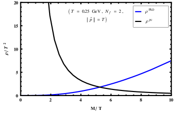
Figure 5: Comparison of the electromagnetic spectral function betwen the perturbative leading order (PLO) and power corrections from $D=4$.

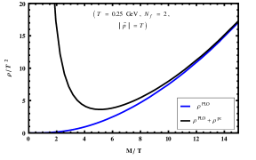
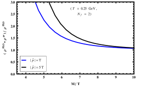
Figure 6: Comparison between $\rho^{\textrm{PLO}}$ in Eq.(46) and $\rho^{\textrm{PLO}}+\rho^{\textrm{pc}}$ in the left panel and their ratio in the right panel.

In figure 6, a comparison (left panel) between the $\rho^{\textrm{PLO}}$ in Eq.(46) and $\rho^{\textrm{PLO}}+\rho^{\textrm{pc}}$ [Eq.(46)+Eq.(44)] and their ratio are displayed, respectively. From the left panel one finds that in the intermediate mass regime, $M\approx 4T$ to $10T$, i.e., (1 to 2.5) GeV, there is a clear indication of enhancement in the electromagnetic spectral function due to the leading order power corrections in $D=4$ dimension. This is also reflected in the ratio plot in the right panel. Both plot assures that the power corrections becomes important in the intermediate mass range of the electromagnetic spectral function.

For convenience the PLO spectral function in Eq.(46) can be simplified in the OPE limit as

$$\rho^{\textrm{PLO}}_{\textrm{sim}}(p) = \frac{N_{c}N_{f}p^{2}}{4\pi^{2}}.$$ (48)

and is also justified through Fig. 7.

The total spectral function with the power correction in the OPE limit can now be written as

$$\rho(p)|^{OPE} = \rho^{\textrm{PLO}}_{\textrm{sim}}(p)+\rho^{\textrm{pc}}(p)$$ (49)

$$= \frac{N_{c}N_{f}p^{2}}{4\pi^{2}}-\frac{16N_{c}N_{f}\alpha_{s}}{9\pi p^{2}}\left(1-4\frac{\omega^{2}}{p^{2}}\right)\left[\frac{8}{3}\Big{\langle}\Theta_{f}^{00}\Big{\rangle}_{T}-\frac{1}{2}\Big{\langle}\Theta_{g}^{00}\Big{\rangle}_{T}\right].$$

Now we note that the virtual photon will decay into two leptons and the features observed in the electromagnetic spectral function will also be reflected in the dilepton production rate, which will be discussed in the next section.

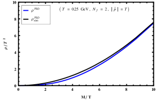
Figure 7: Comparison between $\rho^{\textrm{PLO}}$ in Eq.(46) and simplified one $\rho^{\textrm{PLO}}_{\textrm{sim}}$ in Eq.(48).

6 Dilepton Rate

The modified PLO differential dilepton production rate in presence of leading power correction in OPE with $D=4$ is now obtained in a compact form by combining Eqs.(50) and (49) for $N_{f}=2$ as

$${\frac{dR}{d^{4}xd^{4}p}}\Bigg{|}^{\textrm{OPE}} = \frac{5\alpha^{2}_{\textrm{e}m}}{27\pi^{2}M^{2}}n_{B}\left(\omega\right)$$ (50)

$$\times\left[\frac{N_{c}p^{2}}{4\pi^{2}}-\frac{16N_{c}\alpha_{s}}{9\pi p^{2}}\left(1-4\frac{\omega^{2}}{p^{2}}\right)\left(\frac{8}{3}\Big{\langle}\Theta_{f}^{00}\Big{\rangle}-\frac{1}{2}\Big{\langle}\Theta_{g}^{00}\Big{\rangle}\right)\right],$$

where we have used $\sum_{f}q_{f}^{2}=5/9$, for massless $u$ and $d$ quarks. The leading power corrections within OPE in $D=4$ dimension is of ${\cal O}(\alpha^{2}_{em}\alpha_{s})$ to the PLO of ${\cal O}(\alpha^{2}_{em})$.

In Fig. 8, a comparison is displayed among various thermal dilepton rates as a function of $\omega/T$ with $T=250$ MeV and zero external three momentum. The various dilepton rates considered here are Born (PLO) Greiner:2010zg ; Cleymans:1992gb , PLO plus power corrections within OPE in Eq.(50), LQCD Ding:2010ga ; Ding:2016hua and Polyakov Loop (PL) based models in an effective QCD approach Islam:2014sea ; Gale:2014dfa . The dilepton rate from PL based models and LQCD for $\omega/T>4$ becomes simply perturbative in nature whereas it is so for $\omega/T\geq 10$ in case of the PLO with power corrections in OPE. For $\omega/T>4$, in PL based models the confinement effect due to Polyakov loop becomes very weak whereas in LQCD the spectral function is replaced by the PLO one. On the other hand the enhancement of the dilepton rate at low energy ($\omega/T<4$) for both PL based models and LQCD is due to the presence of some nonperturbative effects (e.g., residual confinement effect etc) whereas in that region the power corrections within OPE is not applicable. However, in the intermediate domain ($4<\omega/T<10$) the dilepton rate is enhanced compared to PL based models and LQCD due to the presence of the nonperturbative composite quark and gluon operators that incorporates power corrections within OPE in $D=4$. We note that the power corrections in OPE considered here may play an important role for intermediate mass dilepton spectra from high energy heavy-ion collisions in RHIC and LHC.

Figure 8: Comparison between different dilepton rates as a function of $\omega/T$ with $T=250$ MeV, obtained from Lattice simulations Ding:2010ga ; Ding:2016hua , PL based model calculations Islam:2014sea ; Gale:2014dfa , Born rate and the nonperturbative power corrections

7 Conclusion

QCD vacuum has a nontrivial structure due to the fluctuations of the quark and gluonic fields which generate some local composite operators of quark and gluon fields, phenomenologically known as condensates. In perturbative approach by definition such condensates do not appear in the observables. However, the nonperturbative dynamics of QCD is evident through the power corrections in physical observables by considering the nonvanishing vacuum expectation values of such local quark and gluonic composite operators. In this paper we, first, have made an attempt to compute the nonperturbative electromagnetic spectral function in QCD plasma by taking into account the power corrections and the nonperturbative condensates within the framework of the OPE in $D=4$ dimension. The power corrections appears in the in-medium electromagnetic spectral function through the nonanalytic behavior of the current-current correlation function in powers of $p^{-D/2}$ or logarithms in the Wilson coefficients within OPE in $D=4$ dimension. The $c$-numbered Wilson coefficients are computed through Feynman diagrams by incorporating the various condensates. In the massless limit of quarks, the self-energy diagram involving local gluonic operator (topology-II in Fig.4) encounters mass singularity. By exploiting the minimal subtraction through operator mixing this mass singularity cancels out, which renders the Wilson coefficients free from any infrared singularity and hence finite. This result is in conformity with the RGE analysis.

The lepton pairs are produced through the electromagnetic interaction in every stage of the hot and dense medium created in high energy heavy-ion collisions. They are considered to be an important probe of QGP formation because they leave, immediately after their production, the hot and dense medium almost without any interaction. As a spectral property of the electromagnetic spectral function, we then evaluated the differential dilepton production rate from QCD plasma in the intermediate mass range to analyze the effects of power corrections and nonperturbative condensates. The power correction contribution is found to be ${\cal O}(\alpha^{2}_{\textrm{em}}\alpha_{s})$ to the PLO, ${\cal O}(\alpha^{2}_{\textrm{em}})$. Further, we note that the intermediate mass range is considered because the low mass regime ($M\leq 4T\sim 1$ GeV; $T=0.25$ GeV) is prohibited by OPE whereas high mass regime ($M\geq 10T\sim 2.5$ GeV) is well described by the perturbative approach. The intermediate mass range ($4T\leq M\leq 10T$) dilepton in presence of power corrections is found to be enhanced compared to other nonpertubative approaches, i.e., LQCD and effective QCD models. However, we note that the power corrections in differential dilepton rate through OPE considered here could be important to describe the intermediate mass dilepton spectra from heavy-ion collisions.

Finally, we would like to note that there is no estimate available in the present literature for the composite quark and gluon operators (condensates), $\langle\Theta_{g}^{00}\rangle_{T}$ and $\langle\Theta_{f}^{00}\rangle_{T}$, respectively, at finite $T$. Since the present knowledge of these in-medium operators are very meagre in the literature, we have exploited the Stefan-Boltzmann limits for these composite operators to have some limiting information of the nonperturbative effects in the electromagnetic spectral function and its spectral properties. We expect that in near future the computation of such phenomenological quantities should be possible via nonperturbative methods of QCD in lattice and some definite estimation of the power corrections within OPE can only be made for spectral function and its spectral properties.

8 Acknowledgements

The authors would like to acknowledge useful discussions with S. Leupold, S. Mallick, C. A. Islam and N. Haque. AB would specially like to thank P. Chakrabarty for very enlighting discussion. This work is supported by Department of Atomic Energy (DAE), India under the project $``$Theoretical Physics Across The Energy Scale (TPAES)” in Theory Division of Saha Institute of Nuclear Physics.

Appendix A Appendix

A.1 Massless Feynman Integrals

While computing the electromagnetic polarization tensor with gluon condensates, the following Feynman integrals for massless quarks have been used:

$$\mathcal{I}_{mn} = \int\frac{d^{d}k}{(2\pi)^{d}}\frac{1}{(k^{2})^{m}((k-p)^{2})^{n}},$$

$$\mathcal{I}_{mn}^{\mu} = \int\frac{d^{d}k}{(2\pi)^{d}}\frac{k^{\mu}}{(k^{2})^{m}((k-p)^{2})^{n}},$$

$$\mathcal{I}_{mn}^{\mu\nu} = \int\frac{d^{d}k}{(2\pi)^{d}}\frac{k^{\mu}k^{\nu}}{(k^{2})^{m}((k-p)^{2})^{n}}.$$

The primary integrals can be represented as follows,

$$\mathcal{I}_{mn} = \frac{i}{(16\pi^{2})^{\frac{d}{4}}}(-1)^{-m-n}(-p^{2})^{-m-n+\frac{d}{2}}\frac{\Gamma[m+n-\frac{d}{2}]}{\Gamma[m]\Gamma[n]}B\left(\frac{d}{2}-n,\frac{d}{2}-m\right),$$ (51)

$$\mathcal{I}_{mn}^{\mu} = \frac{i}{(16\pi^{2})^{\frac{d}{4}}}(-1)^{-m-n}(-p^{2})^{-m-n+\frac{d}{2}}$$ (52)

$$~{}~{}~{}~{}~{}~{}~{}~{}~{}~{}~{}~{}~{}p^{\mu}\Biggl{\{}\frac{\Gamma[m+n-\frac{d}{2}]\Gamma[1+\frac{d}{2}-m]\Gamma[\frac{d}{2}-n]}{\Gamma[m]\Gamma[n]\Gamma[1+d-m-n]}\Biggr{\}},$$

$$\mathcal{I}_{mn}^{\mu\nu} = \frac{i}{(16\pi^{2})^{\frac{d}{4}}}(-1)^{-m-n}(-p^{2})^{-m-n+\frac{d}{2}}$$ (53)

$$~{}~{}~{}~{}~{}~{}~{}~{}~{}~{}~{}~{}~{}\Biggl{\{}p^{2}g^{\mu\nu}\frac{\Gamma[m+n+2-\frac{d}{2}]\Gamma[1+\frac{d}{2}-m]\Gamma[1+\frac{d}{2}-n]}{2\Gamma[m]\Gamma[n]\Gamma[2+d-m-n]}$$

$$~{}~{}~{}~{}~{}~{}~{}~{}~{}~{}~{}~{}~{}~{}+p^{\mu}p^{\nu}\frac{\Gamma[m+n-\frac{d}{2}]\Gamma[2+\frac{d}{2}-m]\Gamma[\frac{d}{2}-n]}{2\Gamma[m]\Gamma[n]\Gamma[2+d-m-n]}\Biggr{\}}.$$

Now putting $d=4-2\epsilon$, we obtain required results of $\mathcal{I}_{mn},\mathcal{I}_{mn}^{\mu}$ and $\mathcal{I}_{mn}^{\mu\nu}$ for some given values of $m$ and $n$ needed for our purpose:

$$\mathcal{I}_{12} = \mu^{-\epsilon}\frac{i}{16\pi^{2}}\frac{1}{p^{2}}\left(-\frac{1}{\tilde{\epsilon}}\right),$$

$$\mathcal{I}_{22} = \mu^{-\epsilon}\frac{i}{16\pi^{2}}\frac{1}{p^{4}}2\left(-\frac{2}{\tilde{\epsilon}}-2\right),$$

$$\mathcal{I}_{22}^{0} = \mu^{-\epsilon}\frac{i}{16\pi^{2}}\frac{p^{0}}{p^{4}}\left(-\frac{1}{\tilde{\epsilon}}-1\right),$$

$$\mathcal{I}_{31}^{0} = \mu^{-\epsilon}\frac{i}{16\pi^{2}}\frac{p^{0}}{p^{4}}\left(-\frac{1}{2\tilde{\epsilon}}-\frac{1}{2}\right),$$

$$\mathcal{I}_{22}^{00} = \mu^{-\epsilon}\frac{i}{16\pi^{2}}\frac{1}{p^{4}}\left[\frac{p^{2}}{2}+\left(-\frac{1}{\tilde{\epsilon}}-2\right)(p^{0})^{2}\right],$$

$$\mathcal{I}_{31}^{00} = \mu^{-\epsilon}\frac{i}{16\pi^{2}}\frac{1}{(p^{2})^{2}}\left[p^{2}\left(-\frac{1}{4\tilde{\epsilon}}-\frac{1}{4}\right)+\frac{(p^{0})^{2}}{2}\right],$$

$$\mathcal{I}_{41}^{00} = \mu^{-\epsilon}\frac{i}{16\pi^{2}}\frac{1}{(p^{2})^{3}}\left[p^{2}\left(\frac{1}{12\tilde{\epsilon}}-\frac{1}{12}\right)+(p^{0})^{2}\left(-\frac{1}{3\tilde{\epsilon}}-\frac{1}{2}\right)\right],$$

where

$$\mu = e^{\frac{\gamma_{E}}{2}}\frac{\Lambda^{2}}{4\pi},$$

$$\frac{1}{\tilde{\epsilon}} = \frac{1}{\epsilon}-\log\left(\frac{-p^{2}}{\Lambda^{2}}\right),$$

with $\mu$ as the renormalization scale, $\Lambda$ as $\overline{\rm MS}$ renormalization scale and $\gamma_{E}$ as Euler-Mascheroni constant.

References

- (1) M. Le Bellac, Thermal field theory, Cambridge University Press, Cambridge (1996).
- (2) H. A. Weldon, Simple Rules for Discontinuities in Finite Temperature Field Theory, Phys. Rev. D28 (1983) 2007.
- (3) H. A. Weldon, Reformulation of finite temperature dilepton production, Phys. Rev. D42 (1990) 2384–2387.
- (4) L. D. McLerran and T. Toimela, Photon and Dilepton Emission from the Quark - Gluon Plasma: Some General Considerations, Phys. Rev. D31 (1985) 545.
- (5) R. C. Hwa and K. Kajantie, Diagnosing Quark Matter by Measuring the Total Entropy and the Photon Or Dilepton Emission Rates, Phys. Rev. D32 (1985) 1109.
- (6) K. Kajantie, J. I. Kapusta, L. D. McLerran, and A. Mekjian, Dilepton Emission and the QCD Phase Transition in Ultrarelativistic Nuclear Collisions, Phys. Rev. D34 (1986) 2746.
- (7) K. Kajantie, M. Kataja, L. D. McLerran, and P. V. Ruuskanen, Transverse Flow Effects in Dilepton Emission, Phys. Rev. D34 (1986) 811.
- (8) J. Cleymans, J. Fingberg, and K. Redlich, Transverse Momentum Distribution of Dileptons in Different Scenarios for the QCD Phase Transition, Phys. Rev. D35 (1987) 2153.
- (9) J. Cleymans and I. Dadic, Lepton pair production from a quark - gluon plasma to first order in alpha-s, Phys. Rev. D47 (1993) 160–172.
- (10) C. Gale and J. I. Kapusta, WHAT IS INTERESTING ABOUT DILEPTON PRODUCTION AT BEVALAC / SIS/ AGS ENERGIES?, Nucl. Phys. A495 (1989) 423C–444C.
- (11) C. Gale and J. I. Kapusta, Dilepton radiation from high temperature nuclear matter, Phys. Rev. C35 (1987) 2107–2116.
- (12) E. Braaten, R. D. Pisarski, and T.-C. Yuan, Production of Soft Dileptons in the Quark - Gluon Plasma, Phys. Rev. Lett. 64 (1990) 2242.
- (13) F. Karsch, M. G. Mustafa, and M. H. Thoma, Finite temperature meson correlation functions in HTL approximation, Phys. Lett. B497 (2001) 249–258, [hep-ph/0007093].
- (14) A. Bandyopadhyay, N. Haque, M. G. Mustafa, and M. Strickland, Dilepton rate and quark number susceptibility with the Gribov action, Phys. Rev. D93 (2016), no. 6 065004, [arXiv:1508.0624].
- (15) C. Greiner, N. Haque, M. G. Mustafa, and M. H. Thoma, Low Mass Dilepton Rate from the Deconfined Phase, Phys. Rev. C83 (2011) 014908, [arXiv:1010.2169].
- (16) P. Aurenche, F. Gelis, R. Kobes, and H. Zaraket, Bremsstrahlung and photon production in thermal QCD, Phys. Rev. D58 (1998) 085003, [hep-ph/9804224].
- (17) M. G. Mustafa, A. Schafer, and M. H. Thoma, Nonperturbative dilepton production from a quark gluon plasma, Phys. Rev. C61 (2000) 024902, [hep-ph/9908461].
- (18) F. Karsch, E. Laermann, P. Petreczky, S. Stickan, and I. Wetzorke, A Lattice calculation of thermal dilepton rates, Phys. Lett. B530 (2002) 147–152, [hep-lat/0110208].
- (19) H. T. Ding, A. Francis, O. Kaczmarek, F. Karsch, E. Laermann, and W. Soeldner, Thermal dilepton rate and electrical conductivity: An analysis of vector current correlation functions in quenched lattice QCD, Phys. Rev. D83 (2011) 034504, [arXiv:1012.4963].
- (20) H.-T. Ding, O. Kaczmarek, and F. Meyer, Thermal dilepton rates and electrical conductivity of the QGP from the lattice, arXiv:1604.0671.
- (21) C. A. Islam, S. Majumder, N. Haque, and M. G. Mustafa, Vector meson spectral function and dilepton production rate in a hot and dense medium within an effective QCD approach, JHEP 02 (2015) 011, [arXiv:1411.6407].
- (22) A. Bandyopadhyay, C. A. Islam and M. G. Mustafa, Electromagnetic spectral properties and Debye screening of a strongly magnetized hot medium, arXiv:1602.06769 [hep-ph].
- (23) N. Sadooghi and F. Taghinavaz, Dilepton production rate in a hot and magnetized quark-gluon plasma, arXiv:1601.04887 [hep-ph].
- (24) K. Tuchin, Magnetic contribution to dilepton production in heavy-ion collisions, Phys. Rev. C 88, 024910 (2013) [arXiv:1305.0545 [nucl-th]].
- (25) C. Gale, Y. Hidaka, S. Jeon, S. Lin, J.-F. Paquet, R. D. Pisarski, D. Satow, V. V. Skokov, and G. Vujanovic, Production and Elliptic Flow of Dileptons and Photons in a Matrix Model of the Quark-Gluon Plasma, Phys. Rev. Lett. 114 (2015) 072301, [arXiv:1409.4778].
- (26) C. A. Islam, S. Majumder, and M. G. Mustafa, Vector meson spectral function and dilepton rate in the presence of strong entanglement effect between the chiral and the Polyakov loop dynamics, Phys. Rev. D92 (2015), no. 9 096002, [arXiv:1508.0406].
- (27) D. K. Srivastava, C. Gale, and R. J. Fries, Large mass dileptons from the passage of jets through quark gluon plasma, Phys. Rev. C67 (2003) 034903, [nucl-th/0209063].
- (28) I. Kvasnikova, C. Gale, and D. K. Srivastava, Production of intermediate mass dileptons in relativistic heavy ion collisions, Phys. Rev. C65 (2002) 064903, [hep-ph/0112139].
- (29) R. Chatterjee, D. K. Srivastava, U. W. Heinz, and C. Gale, Elliptic flow of thermal dileptons in relativistic nuclear collisions, Phys. Rev. C75 (2007) 054909, [nucl-th/0702039].
- (30) M. Laine, NLO thermal dilepton rate at non-zero momentum, JHEP 1311, 120 (2013) doi:10.1007/JHEP11(2013)120 [arXiv:1310.0164 [hep-ph]].
- (31) I. Ghisoiu and M. Laine, Interpolation of hard and soft dilepton rates, JHEP 1410, 83 (2014) doi:10.1007/JHEP10(2014)083 [arXiv:1407.7955 [hep-ph]].
- (32) J. Ghiglieri and G. D. Moore, Low Mass Thermal Dilepton Production at NLO in a Weakly Coupled Quark-Gluon Plasma, JHEP 1412, 029 (2014) doi:10.1007/JHEP12(2014)029 [arXiv:1410.4203 [hep-ph]].
- (33) S. D. Drell and T.-M. Yan, Connection of Elastic Electromagnetic Nucleon Form-Factors at Large Q**2 and Deep Inelastic Structure Functions Near Threshold, Phys. Rev. Lett. 24 (1970) 181–185.
- (34) C. A. Dominguez, M. Loewe, J. C. Rojas, and Y. Zhang, Charmonium in the vector channel at finite temperature from QCD sum rules, Phys. Rev. D81 (2010) 014007, [arXiv:0908.2709].
- (35) C. A. Dominguez, M. Loewe, J. C. Rojas, and Y. Zhang, (Pseudo)Scalar Charmonium in Finite Temperature QCD, Phys. Rev. D83 (2011) 034033, [arXiv:1010.4172].
- (36) PHENIX Collaboration, A. Adare et al., Detailed measurement of the pair continuum in and Au+Au collisions at GeV and implications for direct photon production, Phys. Rev. C81 (2010) 034911, [arXiv:0912.0244].
- (37) E. V. Shuryak, Quark-Gluon Plasma and Hadronic Production of Leptons, Photons and Psions, Phys. Lett. B78 (1978) 150. [Yad. Fiz.28,796(1978)].
- (38) G. Aarts and J. M. Martinez Resco, Transport coefficients, spectral functions and the lattice, JHEP 04 (2002) 053, [hep-ph/0203177].
- (39) O. Kaczmarek and A. Francis, Electrical conductivity and thermal dilepton rate from quenched lattice QCD, J. Phys. G38 (2011) 124178, [arXiv:1109.4054].
- (40) G. Aarts and J. M. Martinez Resco, Continuum and lattice meson spectral functions at nonzero momentum and high temperature, Nucl. Phys. B726 (2005) 93–108, [hep-lat/0507004].
- (41) A. Amato, G. Aarts, C. Allton, P. Giudice, S. Hands and J. I. Skullerud, Electrical conductivity of the quark-gluon plasma across the deconfinement transition, Phys. Rev. Lett. 111, no. 17, 172001 (2013) [arXiv:1307.6763 [hep-lat]].
- (42) G. Aarts, C. Allton, A. Amato, P. Giudice, S. Hands and J. I. Skullerud, Electrical conductivity and charge diffusion in thermal QCD from the lattice, JHEP 1502, 186 (2015) [arXiv:1412.6411 [hep-lat]].
- (43) M. Asakawa, T. Hatsuda, and Y. Nakahara, Maximum entropy analysis of the spectral functions in lattice QCD, Prog. Part. Nucl. Phys. 46 (2001) 459–508, [hep-lat/0011040].
- (44) Y. Nakahara, M. Asakawa, and T. Hatsuda, Hadronic spectral functions in lattice QCD, Phys. Rev. D60 (1999) 091503, [hep-lat/9905034].
- (45) G. Cuniberti, E. De Micheli, and G. A. Viano, Reconstructing the thermal Green functions at real times from those at imaginary times, Commun.Math.Phys. 216 (2001) 59–83, [cond-mat/0109175].
- (46) M. Gell-Mann, R. J. Oakes, and B. Renner, Behavior of current divergences under SU(3) x SU(3), Phys. Rev. 175 (1968) 2195–2199.
- (47) A. I. Vainshtein, V. I. Zakharov, and M. A. Shifman, Gluon condensate and leptonic decays of vector mesons, JETP. Lett. 27 (1978) 60.
- (48) M. J. Lavelle and M. Schaden, Propagators and Condensates in QCD, Phys. Lett. B208 (1988) 297–302.
- (49) M. A. Shifman, A. I. Vainshtein, and V. I. Zakharov, QCD and Resonance Physics. Theoretical Foundations, Nucl. Phys. B147 (1979) 385–447.
- (50) M. A. Shifman, A. I. Vainshtein, and V. I. Zakharov, QCD and Resonance Physics: Applications, Nucl. Phys. B147 (1979) 448–518.
- (51) K. G. Wilson, Nonlagrangian models of current algebra, Phys.Rev. 179 (1969) 1499–1512.
- (52) V. A. Novikov, M. A. Shifman, A. I. Vainshtein, and V. I. Zakharov, OPERATOR EXPANSION IN QUANTUM CHROMODYNAMICS BEYOND PERTURBATION THEORY, Nucl. Phys. B174 (1980) 378–396.
- (53) W. Hubschmid and S. Mallik, OPERATOR EXPANSION AT SHORT DISTANCE IN QCD, Nucl. Phys. B207 (1982) 29–42.
- (54) S. Mallik, Operator Product Expansion in QCD at Short Distance. 2., Nucl. Phys. B234 (1984) 45–60.
- (55) E. Bagan, M. R. Ahmady, V. Elias, and T. G. Steele, Equivalence of plane wave and coordinate space techniques in the operator product expansion, Z. Phys. C61 (1994) 157–170.
- (56) V. Novikov, M. A. Shifman, A. Vainshtein, and V. I. Zakharov, Wilson’s Operator Expansion: Can It Fail?, Nucl.Phys. B249 (1985) 445–471.
- (57) V. Novikov, M. A. Shifman, A. Vainshtein, and V. I. Zakharov, Two-Dimensional Sigma Models: Modeling Nonperturbative Effects of Quantum Chromodynamics, Phys.Rept. 116 (1984) 103.
- (58) S. Narison, QCD as a theory of hadrons from partons to confinement, Camb. Monogr. Part. Phys. Nucl. Phys. Cosmol. 17 (2001) 1, [hep-ph/0205006].
- (59) S. Caron-Huot, Asymptotics of thermal spectral functions, Phys.Rev. D79 (2009) 125009, [arXiv:0903.3958].
- (60) E. V. Shuryak, The QCD vacuum, hadrons and the superdense matter, World Sci. Lect. Notes Phys. 71, 1 (2004) [World Sci. Lect. Notes Phys. 8, 1 (1988)].
- (61) A. I. Bochkarev and M. E. Shaposhnikov, Spectrum of the Hot Hadronic Matter and Finite Temperature QCD Sum Rules, Nucl. Phys. B 268, 220 (1986).
- (62) R. J. Furnstahl, T. Hatsuda and S. H. Lee, Applications of QCD Sum Rules at Finite Temperature, Phys. Rev. D 42, 1744 (1990).
- (63) T. H. Hansson and I. Zahed, Qcd Sum Rules At High Temperature, PRINT-90-0339 (STONY-BROOK).
- (64) A. I. Bochkarev and M. E. Shaposhnikov, The First Order Quark - Hadron Phase Transition in QCD, Phys. Lett. 145B, 276 (1984).
- (65) H. G. Dosch and S. Narison, rho MESON SPECTRUM AT FINITE TEMPERATURE, Phys. Lett. B 203, 155 (1988).
- (66) A. V. Smilga, CALCULATION OF THE DEGREE CORRECTIONS IN FIXED POINT GAUGE. (IN RUSSIAN), Sov.J.Nucl.Phys. 35 (1982) 271–277.
- (67) L. J. Reinders, H. Rubinstein, and S. Yazaki, Hadron Properties from QCD Sum Rules, Phys. Rept. 127 (1985) 1.
- (68) S. Mallik, Operator product expansion at finite temperature, Phys.Lett. B416 (1998) 373–378, [hep-ph/9710556].
- (69) D. Antonov, Heavy-quark condensate at zero and finite temperatures for various forms of the short-distance potential, Nucl.Phys.Proc.Suppl. 152 (2006) 144–147, [hep-ph/0411066].
- (70) G. Basar, D. E. Kharzeev, and E. V. Shuryak, Magneto-sonoluminescence and its signatures in photon and dilepton production in relativistic heavy ion collisions, Phys. Rev. C90 (2014), no. 1 014905, [arXiv:1402.2286].
- (71) P. Pascual and E. de Rafael, Gluonic Corrections to Quark Vacuum Condensate Contributions to Two Point Functions in QCD, Z. Phys. C12 (1982) 127.
- (72) M. E. Peskin and D. V. Schroeder, An Introduction to Quantum Field Theory [Addison-Wesley Advanced Book Program, 1995].
- (73) S. Generalis and D. J. Broadhurst, The Heavy Quark Expansion and QCD Sum Rules for Light Quarks, Phys.Lett. B139 (1984) 85.
- (74) D. J. Broadhurst and S. Generalis, CAN MASS SINGULARITIES BE MINIMALLY SUBTRACTED?, Phys.Lett. B142 (1984) 75.
- (75) S. N. Nikolaev and A. V. Radyushkin, Vacuum Corrections to QCD Charmonium Sum Rules: Basic Formalism and O () Results, Nucl. Phys. B213 (1983) 285–304.
- (76) S. N. Nikolaev and A. V. Radyushkin, QCD CHARMONIUM SUM RULES UP TO O (G**4) ORDER. (IN RUSSIAN), Phys. Lett. B124 (1983) 243–246.
- (77) S. N. Nikolaev and A. V. Radyushkin, Method for Computing Higher Gluonic Power Corrections to QCD Charmonium Sum Rules, Phys. Lett. B110 (1982) 476. [Erratum: Phys. Lett.B116,469(1982)].
- (78) A. Grozin, Methods of calculation of higher power corrections in QCD, Int.J.Mod.Phys. A10 (1995) 3497–3529, [hep-ph/9412238].
- (79) D. J. Broadhurst and S. C. Generalis, DIMENSION EIGHT CONTRIBUTIONS TO LIGHT QUARK QCD SUM RULES, Phys. Lett. B165 (1985) 175–180.
- (80) S. Zschocke, T. Hilger, and B. Kampfer, In-medium operator product expansion for heavy-light-quark pseudoscalar mesons, Eur.Phys.J. A47 (2011) 151, [arXiv:1112.2477].
- (81) J. Beringer et al. (Particle Data Group), Phys. Rev. D 86, 010001 (2012)