Two-dimensional collective Hamiltonian for chiral and wobbling modes

Abstract

A two-dimensional collective Hamiltonian (2DCH) on both azimuth and polar motions in triaxial nuclei is proposed to investigate the chiral and wobbling modes. In the 2DCH, the collective potential and the mass parameters are determined from three-dimensional tilted axis cranking (TAC) calculations. The broken chiral and signature symmetries in the TAC solutions are restored by the 2DCH. The validity of the 2DCH is illustrated with a triaxial rotor ($\gamma=-30^{\circ}$) coupling to one $h_{11/2}$ proton particle and one $h_{11/2}$ neutron hole. By diagonalizing the 2DCH, the angular momenta and energy spectra are obtained. These results agree with the exact solutions of the particle rotor model (PRM) at high rotational frequencies. However, at low frequencies, the energies given by the 2DCH are larger than those by the PRM due to the underestimation of the mass parameters. In addition, with increasing angular momentum, the transitions from the chiral vibration to chiral rotation and further to longitudinal wobbling motion have been presented in the 2DCH.

I Introduction

The investigation of various exotic shapes in the atomic nucleus is a long-standing subject in nuclear physics. The observations of chiral doublet bands and wobbling bands provide direct evidence for the stable triaxiality of nuclei. Nuclear chirality was first predicted in 1997 by Frauendorf and Meng Frauendorf and Meng (1997). Experimentally, more than 30 candidate chiral nuclei have been reported in the $A\sim 80$, $100$, $130$, and $190$ mass regions. For more details see, e.g., Refs. Meng et al. (2008); Meng and Zhang (2010); Meng et al. (2014); Bark et al. (2014). The wobbling motion was originally suggested by Bohr and Mottelson in the 1970s Bohr and Mottelson (1975), and has been found mainly in the $A\sim 160$ mass region Odegaard et al. (2001); Amro et al. (2003); Schönwaßer et al. (2003); Bringel et al. (2005); Hartley et al. (2009), and very recently in the $A\sim 130$ region Matta et al. (2015).

Theoretically, many approaches have been developed to investigate nuclear chirality and wobbling motion, such as the particle rotor model (PRM) Frauendorf and Meng (1997); Peng et al. (2003); Koike et al. (2004); Zhang et al. (2007); Higashiyama and Yoshinaga (2007); Qi et al. (2009); Chen et al. (2010); Lawrie and Shirinda (2010); Rohozinski et al. (2011); Shirinda and Lawrie (2012); Zhang and Chen (2016); Bohr and Mottelson (1975); Hamamoto (2002); Hamamoto and Mottelson (2003); Frauendorf and Dönau (2014); Shi and Chen (2015), the tilted axis cranking model (TAC) Frauendorf and Meng (1997); Dimitrov et al. (2000); Olbratowski et al. (2004, 2006); Matta et al. (2015), the tilted axis cranking plus random phase approximation (TAC+RPA) Mukhopadhyay et al. (2007); Almehed et al. (2011); Shimizu and Matsuzaki (1995); Matsuzaki et al. (2002); Matsuzaki et al. (2004a, b); Matsuzaki and Ohtsubo (2004); Shimizu et al. (2005, 2008); Shoji and Shimizu (2009); Frauendorf and Dönau (2015), the interacting boson fermion-fermion model (IBFFM) Brant et al. (2004), the pair truncated shell model (PTSM) Higashiyama et al. (2005), and the projected shell model (PSM) Bhat et al. (2014). The PRM is a quantal model, where the spin is a good quantum number and the quantum tunnelings between the partner bands are obtained automatically. However, it requires some physical quantities, such as the quadrupole deformation parameters and the moments of inertia, as its inputs. In addition, the separation between the single particles and the rotor is sometimes obscure. The TAC is based on the mean-field approximation, and it can be easily extended to treat multi-quasiparticle configurations. However, to describe the chiral or wobbling partners is beyond the scope of the TAC. Thus, the TAC+RPA going beyond the mean-field approximation was developed, but it is restricted to only small amplitude motions such as chiral vibrations or harmonic wobbling modes.

Recently, a collective Hamiltonian (CH) method based on the TAC approach was constructed and applied to the description of chiral vibration and rotation for the system with one $h_{11/2}$ proton particle and one $h_{11/2}$ neutron hole coupled to a triaxial rotor Chen et al. (2013). This CH introduces the orientation of the rotational axis, the azimuth angle $\varphi$, as a dynamical variable; it differs from the Bohr Hamiltonian Bohr and Mottelson (1975) where the deformation parameters $\beta$ and $\gamma$ and the Euler angles $\bm{\Omega}$ are the collective coordinates. It was found that the CH achieves nice agreement with the exact solutions of the PRM for the energy spectra of the chiral partners Chen et al. (2013); Chen (2015). Similar successes have also been achieved for the wobbling motions in the simple, longitudinal, and transverse wobblers Chen et al. (2014).

In principle, the orientation of a rotational axis in triaxial nuclei should be parameterized by the azimuth angle $\varphi$ and the polar angle $\theta$ Frauendorf and Meng (1997). However, in the previous studies Chen et al. (2013, 2014), only the dynamical motions along the $\varphi$ direction was considered, i.e., a one-dimensional collective Hamiltonian (1DCH). It was constructed with a one-dimensional collective potential $V(\varphi)$, which is determined by minimizing the total Routhian $E^{\prime}(\theta,\varphi)$ with respect to $\theta$ at each given value of $\varphi$. Despite the successes of the 1DCH, it is interesting to extend the collective Hamiltonian to two dimensions, by considering both $\theta$ and $\varphi$ as collective variables, and to explore the related new physics.

In this work, the collective potential and the mass parameters in the two-dimensional collective Hamiltonian (2DCH) are extracted from the TAC calculations. As an example, the developed 2DCH will be applied for a system with one $h_{11/2}$ proton particle and one $h_{11/2}$ neutron hole coupled to a triaxial rotor with the triaxial deformation parameter $\gamma=-30^{\circ}$. The obtained results will be compared with those obtained by the 1DCH and the exact solutions calculated by the PRM.

This paper is organized as follows. In Sec. II, the construction and solution of the 2DCH are introduced based on the TAC solutions. The numerical details are given in Sec. III. In Sec. IV, the calculated results from the 2DCH are presented and discussed in details. Finally, the summary and perspective are given in Sec. V.

II Theoretical framework

II.1 Two dimensional collective Hamiltonian

The collective Hamiltonian has a solid microscopic basis and can be derived by the generator coordinate method (GCM) Ring and Schuck (1980), the adiabatic time-dependent Hartree-Fock (ATDHF) method Baranger and Kumar (1968); Ring and Schuck (1980), or the adiabatic self-consistent collective coordinate (ASCC) method Matsuo et al. (2000); Matsuyanagi et al. (2010). The ASCC method was developed based on the self-consistent collective coordinate (SCC) method formulated by Marumori et al. Marumori et al. (1980), who aimed to extract the optimal collective path, maximally decoupled from non-collective degrees of freedom, from the TDHF phase space of large dimension in a fully self-consistent manner. By introducing the adiabatic approximation for the collective momenta, one can expand the collective states in the SCC equations with respect to the collective momenta, and obtain the ASCC equations Matsuo et al. (2000). Solving the ASCC equations, the collective potential and the mass parameters can be obtained to construct the collective Hamiltonian.

According to the ASCC method, the collective Hamiltonian is defined as the expectation of the total energy in the collective states, given by Matsuo et al. (2000)

$$\mathcal{H}(q,p) =\langle\phi(q,p)|\hat{H}|\phi(q,p)\rangle$$

$$=\frac{1}{2}\sum_{ij}B^{-1}_{ij}(q)p_{i}p_{j}+\mathcal{V}(q)$$

$$=\frac{1}{2}\sum_{ij}B_{ij}(q)\dot{q}_{i}\dot{q}_{j}+\mathcal{V}(q),$$ (1)

where $q$ and $p$ are the collective coordinates and momenta, respectively, and the adiabatic assumption of the collective motion has been introduced Matsuo et al. (2000). The collective potential $\mathcal{V}(q)$ and the mass parameters $B_{ij}(q)$ are expressed as functions of the collective coordinates and can be calculated by

$$\mathcal{V}(q)=\mathcal{H}(q,p)|_{p=0},\quad B_{ij}^{-1}(q)=\frac{\partial^{2}\mathcal{H}(q,p)}{\partial p_{i}\partial p_{j}}\Big{|}_{p=0}.$$ (2)

It has been mentioned that the orientation of a rotational axis in triaxial nuclei could be parametrized by the azimuth angle $\varphi$ and the polar angle $\theta$. Thus, to describe the chiral and wobbling modes, the collective coordinates are chosen as $\theta$ and $\varphi$. Correspondingly, the form of the collective Hamiltonian is written as

$$\mathcal{H}(\theta,\varphi) =\mathcal{H}_{\rm kin}(\theta,\varphi)+\mathcal{V}(\theta,\varphi)$$ (3)

$$=\frac{1}{2}B_{\theta\theta}\dot{\theta}^{2}+\frac{1}{2}B_{\theta\varphi}\dot{\theta}\dot{\varphi}+\frac{1}{2}B_{\varphi\theta}\dot{\varphi}\dot{\theta}+\frac{1}{2}B_{\varphi\varphi}\dot{\varphi}^{2}+\mathcal{V}(\theta,\varphi),$$ (4)

in which $\mathcal{V}(\theta,\varphi)$ is the collective potential in the $\theta$-$\varphi$ plane, and $B_{\theta\theta}$, $B_{\theta\varphi}$, $B_{\varphi\theta}$, and $B_{\varphi\varphi}$ are the corresponding mass parameters.

Making use of the general Pauli prescription Pauli (1933), the quantal collective Hamiltonian reads

$$\hat{\mathcal{H}}(\theta,\varphi) =-\frac{\hbar^{2}}{2\sqrt{w}}\Big{[}\frac{\partial}{\partial\varphi}\frac{B_{\theta\theta}}{\sqrt{w}}\frac{\partial}{\partial\varphi}-\frac{\partial}{\partial\varphi}\frac{B_{\varphi\theta}}{\sqrt{w}}\frac{\partial}{\partial\theta}-\frac{\partial}{\partial\theta}\frac{B_{\theta\varphi}}{\sqrt{w}}\frac{\partial}{\partial\varphi}+\frac{\partial}{\partial\theta}\frac{B_{\varphi\varphi}}{\sqrt{w}}\frac{\partial}{\partial\theta}\Big{]}+V(\theta,\varphi),$$ (5)

in which $w$ is the determinant of the mass parameter tensor,

$$w=\det B=\left|\begin{array}[]{cc}B_{\theta\theta}&B_{\theta\varphi}\\ B_{\varphi\theta}&B_{\varphi\varphi}\\ \end{array}\right|=B_{\theta\theta}B_{\varphi\varphi}-B_{\theta\varphi}B_{\varphi\theta}.$$ (8)

As a result, the integral volume element in the collective space is

$$\int d\tau_{\rm coll}=\int_{0}^{\pi}d\theta\int_{-\pi/2}^{\pi/2}d\varphi\sqrt{w}=\int_{0}^{\pi}d\theta\int_{-\pi/2}^{\pi/2}d\varphi\sqrt{B_{\varphi\varphi}B_{\theta\theta}-B_{\varphi\theta}B_{\theta\varphi}}.$$ (9)

Here, it should be noted that the collective Hamiltonian is applied in the rotating frame with a given rotational frequency $\omega$. Namely, for a given $\omega$, we will first determine the collective parameters from the TAC model, and then solve the collective Hamiltonian to obtain the collective energy levels and wave functions.

II.2 Collective potential

The collective potential $V(\theta,\varphi)$ in the 2DCH in Eq. (5) is calculated by the TAC model Chen et al. (2013). We consider a system of one $h_{11/2}$ proton particle and one $h_{11/2}$ neutron hole coupled to a triaxial rotor. The cranking Hamiltonian reads

$$\hat{h}^{\prime} =\hat{h}_{\rm def}-\bm{\omega}\cdot\hat{\bm{j}},$$ (10)

$$\hat{\bm{j}} =\hat{\bm{j}}_{\pi}+\hat{\bm{j}}_{\nu},$$ (11)

$$\bm{\omega} =(\omega\sin\theta\cos\varphi,\omega\sin\theta\sin\varphi,\omega\cos\theta).$$ (12)

The Hamiltonian of the deformed field is the sum of the proton and neutron single-particle Hamiltonian as $\hat{h}_{\rm def}=\hat{h}_{\rm def}^{\rm\pi}+\hat{h}_{\rm def}^{\rm\nu}$. Here, $\hat{h}_{\rm def}^{\rm\pi(\nu)}$ is taken as a triaxial single-$j$ shell Hamiltonian

$$\hat{h}_{\rm def}^{\rm\pi(\nu)}=\frac{1}{2}C_{\pi(\nu)}\Big{\{}(\hat{j}_{3}^{2}-\frac{j(j+1)}{3})\cos\gamma+\frac{1}{2\sqrt{3}}(\hat{j}_{+}^{2}+\hat{j}_{-}^{2})\sin\gamma\Big{\}}$$ (13)

with the positive (negative) value of $C_{\pi(\nu)}$ referring to particles (holes), and the triaxial deformation parameter $\gamma$.

The TAC solutions are obtained self-consistently by minimizing the total Routhian surface Frauendorf and Meng (1996, 1997)

$$E^{\prime}(\theta,\varphi)=\langle h^{\prime}\rangle-\frac{1}{2}\sum_{k=1}^{3}\mathcal{J}_{k}\omega_{k}^{2}$$ (14)

with respect to the tilted angles $\theta$ and $\varphi$, where the moments of inertia of the irrotational flow type Ring and Schuck (1980) are adopted, i.e.,

$$\mathcal{J}_{k}=\mathcal{J}_{0}\sin^{2}\Big{(}\gamma-\displaystyle\frac{2\pi}{3}k\Big{)},$$ (15)

with $\mathcal{J}_{0}$ as an input parameter.

It should be noted that in Ref. Chen et al. (2013), the 1DCH was constructed with the collective potential $V(\varphi)$, which is obtained by minimizing the total Routhian in Eq. (14) with respect to $\theta$ at each given value of $\varphi$. Here, in the 2DCH, one needs $V(\theta,\varphi)$ in the full ($\theta$, $\varphi$) plane. The obtained total Routhian $E^{\prime}(\theta,\varphi)$ is the collective potential $V(\theta,\varphi)$.

II.3 Mass parameters

A fully self-consistent solution of the mass parameters within the ASCC method is very time-consuming Matsuo et al. (2000). However, if the residual interaction in the Hamiltonian $\hat{H}$ is neglected, a simple formalism for mass parameter can be obtained, which corresponds to the cranking formula Ring and Schuck (1980):

$$B_{\theta\theta} =2\sum_{mi}\frac{\Big{|}\langle m|\displaystyle\frac{\partial\bm{\omega}}{\partial\theta}\cdot\hat{\bm{j}}|i\rangle\Big{|}^{2}}{(\varepsilon_{m}-\varepsilon_{i})^{3}},$$ (16)

$$B_{\theta\varphi} =2\sum_{mi}\frac{\langle m|\displaystyle\frac{\partial\bm{\omega}}{\partial\theta}\cdot\hat{\bm{j}}|i\rangle\langle i|\displaystyle\frac{\partial\bm{\omega}}{\partial\varphi}\cdot\hat{\bm{j}}|m\rangle}{(\varepsilon_{m}-\varepsilon_{i})^{3}},$$ (17)

$$B_{\varphi\theta} =2\sum_{mi}\frac{\langle m|\displaystyle\frac{\partial\bm{\omega}}{\partial\varphi}\cdot\hat{\bm{j}}|i\rangle\langle i|\displaystyle\frac{\partial\bm{\omega}}{\partial\theta}\cdot\hat{\bm{j}}|m\rangle}{(\varepsilon_{m}-\varepsilon_{i})^{3}},$$ (18)

$$B_{\varphi\varphi} =2\sum_{mi}\frac{\Big{|}\langle m|\displaystyle\frac{\partial\bm{\omega}}{\partial\varphi}\cdot\hat{\bm{j}}|i\rangle\Big{|}^{2}}{(\varepsilon_{m}-\varepsilon_{i})^{3}}.$$ (19)

Here, the $\varepsilon_{m}$ and $\varepsilon_{i}$ are the energies of the single-particle states $|m\rangle$ and $|i\rangle$, respectively. They are obtained by diagonalizing the cranking Hamiltonian $\hat{h}^{\prime}$ in Eq. (10). Here, $m$ denotes the particle states and $i$ the hole states. The matrix elements are respectively

$$\langle m|\frac{\partial\bm{\omega}}{\partial\theta}\cdot\bm{j}|i\rangle =\omega\Big{(}\cos\theta\cos\varphi\langle m|\hat{j}_{1}|i\rangle+\cos\theta\sin\varphi\langle m|\hat{j}_{2}|i\rangle-\sin\theta\langle m|\hat{j}_{3}|i\rangle\Big{)},$$ (20)

$$\langle m|\frac{\partial\bm{\omega}}{\partial\varphi}\cdot\bm{j}|i\rangle =\omega\Big{(}-\sin\theta\sin\varphi\langle m|\hat{j}_{1}|i\rangle+\sin\theta\cos\varphi\langle m|\hat{j}_{2}|i\rangle\Big{)}.$$ (21)

One easily finds that $B_{\theta\theta}$ and $B_{\varphi\varphi}$ are symmetric, while $B_{\theta\varphi}=B_{\varphi\theta}$ is antisymmetric, under the transformation $\varphi\to-\varphi$ or $\theta\to\pi-\theta$.

Note that in our previous study Chen et al. (2013), the mass parameter $B_{\varphi\varphi}$ is derived with the adiabatic perturbation theory by assuming a harmonic motion of $\varphi$ with the vibrational frequency $\Omega_{\varphi}$: $\ddot{\varphi}=-\Omega_{\varphi}^{2}\varphi$. In such way, we obtain the corresponding mass parameter

$$B_{\varphi\varphi}=2\sum_{mi}\frac{(\varepsilon_{m}-\varepsilon_{i})\Big{|}\langle m|\displaystyle\frac{\partial\bm{\omega}}{\partial\varphi}\cdot\hat{\bm{j}}|i\rangle\Big{|}^{2}}{[(\varepsilon_{m}-\varepsilon_{i})^{2}-\hbar^{2}\Omega_{\varphi}^{2}]^{2}}.$$ (22)

This is the same as Eq. (19) with a vanishing vibrational frequency $\hbar\Omega_{\varphi}$, which is associated with the neglect of the residual interaction in the Hamiltonian $\hat{H}$ in the derivation of Eq. (19).

Here we would like to add some discussions for the mass parameters presented in Eqs. (16)-(19) and (22). In Ref. Chen et al. (2013), we have proposed to calculate the vibrational frequency $\Omega_{\varphi}$ in Eq. (22). Namely, (a) for a potential with two minima, the case of chiral rotation, it can be approximately taken as zero since the barrier penetration between the left-handed and right-handed states is low; (b) for a potential with one minimum, the case of chiral vibration, it is calculated by evaluating the curvature of the potential $K$, and self-consistently solving the equation $B(\Omega_{\varphi})=K/\Omega_{\varphi}^{2}$. Thus the vanishing of vibration frequencies in Eqs. (16)-(19) is a good approximation for the potential with two minima (at the high rotational frequency regions), while could lead to an underestimation for the potential with one minimum (at the low rotational frequency regions). In addition, it is noted that the numerator in the formulas of the mass parameters in Eqs. (16)-(19) and (22) are proportional to $\omega^{2}$ as shown in Eqs. (20)-(21). Therefore, in general, if $\omega$ is very small, the mass parameter would be rather small.

II.4 Basis space

It is easy to verify that the 2DCH in Eq. (5) is invariant under the transformation $\varphi\to-\varphi$ or $\theta\to\pi-\theta$. We define two operators $\hat{P}_{\theta}$ and $\hat{P}_{\varphi}$ associated with the transformations $\varphi\to-\varphi$ and $\theta\to\pi-\theta$, respectively. The eigenvalues of the $\hat{P}_{\theta}$ and $\hat{P}_{\varphi}$ are “$+$” or “$-$”, depending on whether the state is symmetric or antisymmetric with respect to the transformations. Therefore, the 2DCH can be diagonalized in the four individual subspaces.

In each subspace, the bases used to diagonalize the two dimensional collective Hamiltonian are denoted as $\psi_{mn}^{(P_{\theta}P_{\varphi})}(\theta,\varphi)$, where $P_{\theta}$ ($P_{\varphi}$) denotes the eigenvalues of the $\hat{P}_{\theta}$ ($\hat{P}_{\varphi}$). The bases are chosen as the Fourier series

$$\psi_{mn}^{(++)}(\theta,\varphi) =\sqrt{\frac{4}{\pi^{2}(1+\delta_{m0})(1+\delta_{n0})}}\frac{\cos 2m\theta\cos 2n\varphi}{w^{1/4}},\quad m,n\geq 0,$$ (23)

$$\psi_{mn}^{(+-)}(\theta,\varphi) =\sqrt{\frac{4}{\pi^{2}(1+\delta_{m0})}}\frac{\cos 2m\theta\sin 2n\varphi}{w^{1/4}},\quad m\geq 0,n\geq 1,$$ (24)

$$\psi_{mn}^{(-+)}(\theta,\varphi) =\sqrt{\frac{4}{\pi^{2}(1+\delta_{n0})}}\frac{\sin 2m\theta\cos 2n\varphi}{w^{1/4}},\quad m\geq 1,n\geq 0,$$ (25)

$$\psi_{mn}^{(--)}(\theta,\varphi) =\sqrt{\frac{4}{\pi^{2}}}\frac{\sin 2m\theta\sin 2n\varphi}{w^{1/4}},\quad m,n\geq 1.$$ (26)

One can easily prove that these bases fulfill the normalization conditions with the collective measure in Eq. (9), and satisfy the following periodic boundary conditions

$$\psi_{mn}^{(P_{\theta}P_{\varphi})}(\theta,\varphi) =\psi_{mn}^{(P_{\theta}P_{\varphi})}(\theta+\pi,\varphi),$$

$$\psi_{mn}^{(P_{\theta}P_{\varphi})}(\theta,\varphi) =\psi_{mn}^{(P_{\theta}P_{\varphi})}(\theta,\varphi+\pi).$$ (27)

Finally, we obtain the wave functions of the collective Hamiltonian

$$\Psi(\theta,\varphi) =\sum_{mn}c_{mn}^{P_{\theta}P_{\varphi}}\psi_{mn}^{(P_{\theta}P_{\varphi})}(\theta,\varphi),$$ (28)

where the expansion coefficients $c_{mn}^{P_{\theta}P_{\varphi}}$ are obtained by diagonalizing the 2DCH.

III Numerical details

In the present work, we consider a system with the particle-hole configuration $\pi(1h_{11/2})^{1}\otimes\nu(1h_{11/2})^{-1}$ with triaxial deformation parameter $\gamma=-30^{\circ}$. The 1, 2, and 3 axes correspond to the short ($s$), intermediate ($i$), and long ($l$) axes, respectively. The coupling parameter $C_{\pi(\nu)}$ in the single-$j$ shell Hamiltonian in Eq. (13) is chosen as $C_{\pi}=0.25~{}\mathrm{MeV}$ for the proton particle and $C_{\nu}=-0.25~{}\mathrm{MeV}$ for the neutron hole. The moment of inertia of the triaxial rotor is taken as $\mathcal{J}_{0}=40~{}\hbar^{2}/\mathrm{MeV}$. These numerical details are the same as in Refs. Frauendorf and Meng (1997); Chen et al. (2013).

IV Results and discussion

IV.1 Collective parameters

The collective parameters of the 2DCH, including the collective potential $V(\theta,\varphi)$ and mass parameters $B_{\theta\theta}(\theta,\varphi)$, $B_{\theta\varphi}(\theta,\varphi)$, and $B_{\varphi\varphi}(\theta,\varphi)$, are provided based on the TAC calculations.

IV.1.1 Collective potential

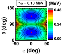
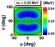
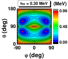
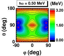
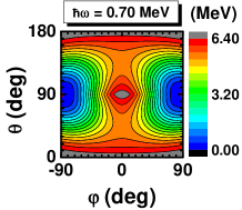
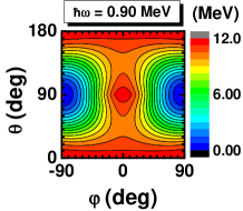
Figure 1: (Color online) Total Routhian surface calculations for one $h_{11/2}$ proton particle and one $h_{11/2}$ neutron hole coupled to a triaxial rotor with $\gamma=-30^{\circ}$ at the frequencies $\hbar\omega=0.10$, 0.20, 0.30, 0.50, 0.70, 0.90 MeV. All energies are normalized with respect to the absolute minima (stars). Note that different scales have been used in different panels. In each panel, twenty contour lines are shown.

The potential energy surfaces in the rotating frame, i.e., the total Routhian $E^{\prime}(\theta,\varphi)$ in Eq. (14) as functions of $\theta$ and $\varphi$, are shown in Fig. 1 at the frequencies $\hbar\omega=0.10$, 0.20, 0.30, 0.50, 0.70, and 0.90 MeV. The present results are consistent with those presented in Refs. Frauendorf and Meng (1997); Chen et al. (2013).

One can see in Fig. 1 that all the potential energy surfaces are symmetric with respect to the $\varphi=0^{\circ}$ and $\theta=90^{\circ}$ lines. This is due to the $D_{2}$ symmetry for a quadrupole deformed nucleus. With the increase of frequency, the minima in the potential energy surfaces change from $\varphi=0^{\circ}$ to $\varphi\neq 0^{\circ}$ ($\hbar\omega\sim 0.20~{}\mathrm{MeV}$), showing that the rotating mode changes from a planar to an aplanar rotation Frauendorf and Meng (1997). When $\hbar\omega\sim 0.70~{}\mathrm{MeV}$, the minima change to $\theta=90^{\circ}$ and $\varphi=\pm 90^{\circ}$, and the yrast rotating mode becomes a principal axis rotation along the $i$ axis.

In addition, it is seen that the potential energy surfaces are rather soft in the direction of $\varphi$ at the low rotational frequencies ($\hbar\omega\leq 0.20$ MeV). In the high frequency region ($\hbar\omega\geq 0.50$ MeV), however, considerable softness is observed also in the $\theta$ direction. This indicates that the fluctuations along the $\theta$ direction would play a remarkable role at high frequencies.

IV.1.2 Mass parameters

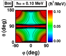
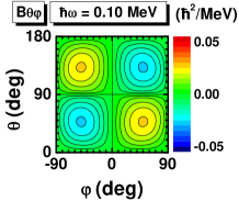
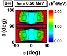
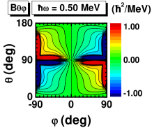
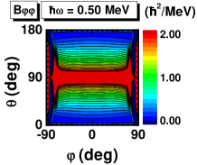
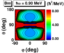
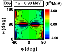
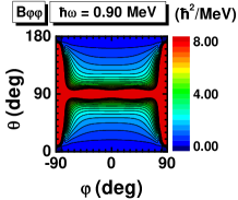
Figure 2: (Color online) The mass parameters $B_{\theta\theta}$, $B_{\theta\varphi}$, and $B_{\varphi\varphi}$ as functions of $\theta$ and $\varphi$ at the frequencies $\hbar\omega=0.10$, 0.50, and 0.90 MeV calculated based on TAC. Note that different scales have been used in different panels. In each panel, twenty contour lines are shown.

The mass parameters in the 2DCH include $B_{\theta\theta}$, $B_{\theta\varphi}$, $B_{\varphi\theta}$, and $B_{\varphi\varphi}$, and they govern the kinetic energy of the collective motion. In the present study, they are calculated with Eqs. (16)-(19), and we show the obtained results in Fig. 2 at $(\theta,\varphi)$ plane for the frequencies $\hbar\omega=0.10$, 0.50, and 0.90 MeV. Here, only $B_{\theta\theta}$, $B_{\theta\varphi}$, and $B_{\varphi\varphi}$ are shown since $B_{\theta\varphi}$ and $B_{\varphi\theta}$ are identical.

In Fig. 2, one can see clearly that $B_{\theta\theta}$ and $B_{\varphi\varphi}$ are symmetric, while $B_{\theta\varphi}$ is antisymmetric with respect to $\varphi=0^{\circ}$ and $\theta=90^{\circ}$. These behaviors, together with the symmetrical collective potential in Fig. 1, ensure the invariance of the collective Hamiltonian with the transformations of $\varphi\to-\varphi$ and $\theta\to 180^{\circ}-\theta$. All the mass parameters $B_{\theta\theta}$, $B_{\theta\varphi}$, and $B_{\varphi\varphi}$ generally increase with frequency, since they are proportional to $\omega^{2}$ as in Eqs. (16)-(19). However, $B_{\theta\theta}$ and $B_{\varphi\varphi}$ behave differently in the $(\theta,\varphi)$ plane. $B_{\theta\theta}$ is more sensitive than $B_{\varphi\varphi}$ in the $\varphi$ direction, while the latter varies more strongly in the $\theta$ direction than the former. Specifically, $B_{\theta\theta}$ ($B_{\varphi\varphi}$) varies in a near-parabolic way with respect to $\varphi$ ($\theta$), and the minimum locates at $\varphi=0^{\circ}$ ($\theta=0^{\circ}$). Note that both $B_{\theta\theta}$ and $B_{\varphi\varphi}$ are considerably large at $\theta\sim 90^{\circ}$ or $\varphi\sim\pm 90^{\circ}$, and such singularities result from the rather small energy differences between the two lowest cranking energy levels in Eqs. (16)-(19). These singularities might disappear by including pairing correlations, which requires the replacement of the denominators in Eqs. (16)-(19) by the sum of two quasiparticle energies.

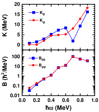
Figure 3: (Color online) The $B_{\theta\theta}$ and $B_{\varphi\varphi}$ and the curvatures $K_{\theta}$ and $K_{\varphi}$ at the minimum of the potential energy surface as functions of rotational frequency.

In Fig. 3, the mass parameters $B_{\theta\theta}$ and $B_{\varphi\varphi}$ and the curvatures $K_{\theta}$ and $K_{\varphi}$ at the minimum of the potential energy surface (PES) as functions of rotational frequency are shown. The curvatures are calculated by

$$K_{\theta}=\frac{\partial^{2}V(\theta,\varphi)}{\partial^{2}\theta}\Big{|}_{\theta_{\min},\varphi_{\min}},\quad K_{\varphi}=\frac{\partial^{2}V(\theta,\varphi)}{\partial^{2}\varphi}\Big{|}_{\theta_{\min},\varphi_{\min}},$$ (29)

where $\theta_{\min}$ and $\varphi_{\min}$ are the values of the $\theta$ and $\varphi$ at the minimum. It is seen that $B_{\theta\theta}$ and $B_{\varphi\varphi}$ at the minimum of the potential energy surface are nearly the same. They increase with rotational frequency up to $\hbar\omega=0.70~{}\rm{MeV}$, and then decrease slightly. It is noted that they change about two orders of magnitude from the low $(\hbar\omega=0.10~{}\rm{MeV})$ to high $(\hbar\omega=0.90~{}\rm{MeV})$ frequencies. This can be understood since the mass parameter is proportional to $\omega^{2}$ as seen in Eqs. (18) and (19). For the curvature $K_{\varphi}$, it first exhibits a decrease behavior up to $\hbar\omega=0.20~{}\rm{MeV}$, and then gradually increases with the increase of rotational frequency. For the $K_{\theta}$, there is a jump from $\hbar\omega=0.60~{}\rm{MeV}$ to $\hbar\omega=0.70~{}\rm{MeV}$. These behaviors are consistent with the picture that the rotating mode changes from a planar to an aplanar rotation (at $\hbar\omega=0.20$ MeV), and to a principal axis rotation (at $\hbar\omega=0.70$ MeV).

IV.2 Collective energy levels and wave functions

IV.2.1 Collective energy levels

The diagonalization of the 2DCH yields the energy levels and wave functions at each cranking frequency. Since the 2DCH is invariant with the transformations $\varphi\to-\varphi$ and $\theta\to\pi-\theta$, one could group the eigenenergies and eigenstates into four categories with different combinations of the symmetries $P_{\theta}$ and $P_{\varphi}$, i.e., $(P_{\theta}P_{\varphi})=(++)$, $(+-)$, $(-+)$, and $(--)$.

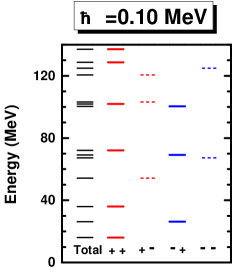
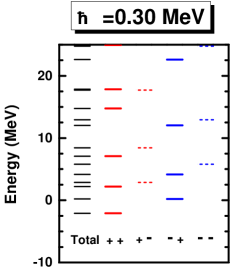
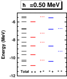
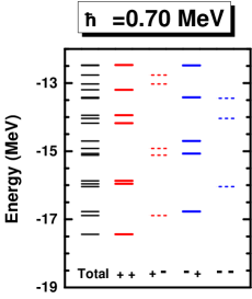
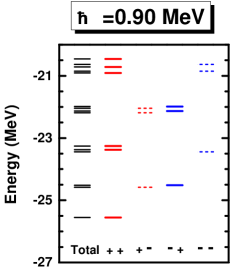
Figure 4: (Color online) Collective energy levels obtained from the two-dimensional collective Hamiltonian at the frequencies $\hbar\omega=0.10$, 0.20, 0.30, 0.50, 0.70, and 0.90 MeV. Note that different scales have been used in different panels.

In Fig. 4, the obtained collective energy levels at the frequencies $\hbar\omega=0.10$, 0.20, 0.30, 0.50, 0.70, and 0.90 MeV are shown (labeled as “Total” in each panel). They can be grouped according to four symmetries $(P_{\theta}P_{\varphi})=(++)$, $(+-)$, $(-+)$, and $(--)$. The lowest energy level corresponds to the zero-phonon oscillation along both the $\theta$ and $\varphi$ directions, and it is always in the group $(++)$. In fact, the energy levels in different groups are associated with different phonon excitation modes. For instance, each energy level in the group $(++)$ is from even-phonon excitations along both the $\theta$ and $\varphi$ directions, while for the group $(--)$, it is from odd-phonon excitations in both directions. Similarly, the energy levels in the group $(+-)$ [$(-+)$] correspond to even (odd) phonons excitations along the $\theta$ direction and an odd (even) ones along the $\varphi$ direction.

One can see in Fig. 4 that the energy levels are sparsely distributed at low rotational frequencies, e.g., $\hbar\omega=0.10$ MeV. It should be kept in mind that the vibrational frequency $\hbar\Omega$ is neglected in the present calculations and, thus, the obtained mass parameters at lower rotational frequencies can be relatively too small (see Sec. II.3). This leads to the extremely high excitation energies at low frequencies. At higher rotational frequencies, although the $\hbar\Omega$ is also neglected, the collective potentials in these cases are with two minima (see Fig. 1) and, thus, the neglect of $\hbar\Omega$ becomes a reasonable approximation.

At $\hbar\omega\leq 0.50$ MeV, the lowest energy state in the group $(+-)$ is higher than that in the group $(-+)$, while they become nearly degenerate at $\hbar\omega\geq 0.70~{}\rm{MeV}$. This indicates that the motion along the $\theta$ direction is more favorable than that of the $\varphi$ direction at low rotational frequencies, while they become comparable at high frequencies. One can understand these behaviors by the collective mass parameters as the variation of the collective potential along the $\theta$ and $\varphi$ directions are comparable. Thus the excitation energies along the $\theta$ and $\varphi$ directions are mainly determined by the kinetic terms. From Fig. 2, we observe that $B_{\varphi\varphi}$ is remarkably smaller than $B_{\theta\theta}$ at low frequencies, and $B_{\varphi\varphi}$ is comparable with $B_{\theta\theta}$ at high frequencies.

IV.2.2 Collective wave functions

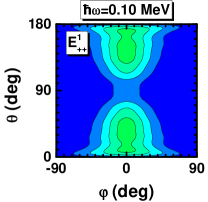
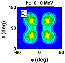
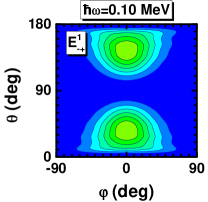
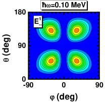
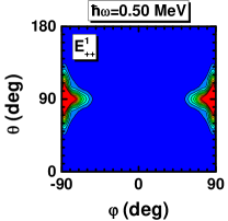
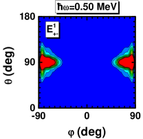
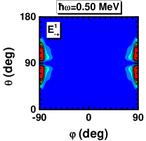
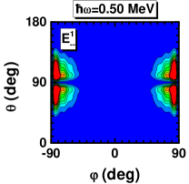
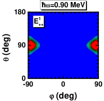
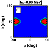
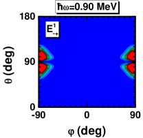
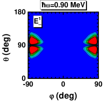
Figure 5: (Color online) The density profiles of of the lowest states in groups $(++)$, $(+-)$, $(-+)$, and $(--)$ at the frequencies $\hbar\omega=0.10$, 0.50, and 0.90 MeV calculated by the 2DCH.

The symmetric features of different energy states are well revealed by their wave functions. In Fig. 5, the probability density distributions of the lowest states in the four groups (labeled as $E_{++}^{1}$, $E_{+-}^{1}$, $E_{-+}^{1}$, and $E_{--}^{1}$, respectively), obtained from the 2DCH for the rotational frequencies $\hbar\omega=0.10$, 0.50, and 0.90 MeV, are shown in the $(\theta,\varphi)$ plane. Here, the probability density distribution is defined according to the collective wave function in Eq. (28) as

$$\rho(\theta,\varphi)=|\Psi(\theta,\varphi)|^{2}\sqrt{w},$$ (30)

which satisfies the normalization condition

$$\int_{0}^{\pi}d\theta\int_{-\pi/2}^{\pi/2}d\varphi\rho(\theta,\varphi)=1.$$ (31)

It is shown in Fig. 5 that the densities are symmetric with respect to $\theta=90^{\circ}$ and $\varphi=0^{\circ}$. This is expected since the broken $P_{\theta}$ and $P_{\varphi}$ symmetries in the TAC solutions have been fully restored in the 2DCH. For $\hbar\omega=0.10~{}\rm{MeV}$, the peak of the density of $E_{++}^{1}$ is located at ($\theta\approx 50^{\circ}$, $\varphi=0^{\circ}$), which corresponds to the region of the minimum in the PES as shown in Fig. 1. The density profiles of $E_{+-}^{1}$ and $E_{-+}^{1}$ are separated into two parts by $\varphi=0^{\circ}$ and $\theta=90^{\circ}$, respectively. This indicates that the one-phonon excitation is mainly along the $\varphi$ direction for $E_{+-}^{1}$ and the $\theta$ one for $E_{-+}^{1}$. As for $E_{--}^{1}$ state, its density profile is separated into four parts, so there are one phonon excitations along both the directions of $\varphi$ and $\theta$. Furthermore, the summation of $E_{+-}^{1}$ and $E_{-+}^{1}$ is very close to $E_{--}^{1}$, and this reveals a weak coupling between the phonon excitations along the $\varphi$ and $\theta$ directions.

The above features can also be found in the obtained density profiles for other rotational frequencies. However, the density profiles of all states at $\hbar\omega=0.50$ and $0.90~{}\rm{MeV}$ exhibit quite different locations of the maxima from those at $\hbar\omega=0.10$ MeV, since the corresponding collective potentials are quite different (see Fig. 1). On the other hand, similar collective potentials and mass parameter distributions have been obtained at $\hbar\omega=0.50$ and $0.90~{}\rm{MeV}$, and this leads to the similarity of the corresponding density profiles at these two rotational frequencies. In such high frequencies, the nuclear yrast mode corresponds to a principal rotation, where the orientation of the total angular momentum is along the intermediate axis with the largest moment of inertia. Therefore, the multi phonon excitation modes are all in the vicinity of the intermediate axis, and these can be regarded as the wobbling motions. One may classify these wobbling motions into two types: $\varphi$ wobbling where the wobbling motion occurs along the $\varphi$ direction, and $\theta$ wobbling along the $\theta$ direction. Here, we would like to emphasize that such a classification is naturally obtained since the $\theta$ and $\varphi$ are treated as the collective degrees of freedom in the collective Hamiltonian. This is analogous to that the concepts of $\beta$ band and $\gamma$ band appear in the Bohr Hamiltonian. In addition, as the $\theta$ and $\varphi$ already appeared separately in the collective Hamiltonian, the wobbling picture appears in the way of oscillations along the $\theta$ or $\varphi$ directions, rather than their combinations. As the $E_{+-}^{1}$ and $E_{-+}^{1}$ are nearly degenerate, as shown in Fig. 4, the $\varphi$-wobbling and the $\theta$-wobbling motions are comparable in magnitude here. This is associated with the fact that, in the present discussed system with $\gamma=-30^{\circ}$, the moments of inertia of the short and long axes are the same, and, as mentioned before, such a system also leads to the similar softness of the potential energy surfaces along the $\varphi$ and $\theta$ directions at high frequencies, as shown in Fig. 1.

IV.3 Comparison of one- and two- dimensional collective Hamiltonians

In this section, taking $\hbar\omega=0.10$, 0.50, and 0.90 MeV as examples, the collective energy levels and the wave functions obtained by the 2DCH will be compared with those obtained by the 1DCH. Here, it should be noted that the results of 1DCH presented here are obtained with the basis states under the periodic boundary condition

$$\psi_{n}^{(+)}(\varphi) =\sqrt{\frac{2}{\pi(1+\delta_{n0})}}\frac{\cos 2n\varphi}{B^{1/4}(\varphi)},\quad n\geq 0,$$

$$\psi_{n}^{(-)}(\varphi) =\sqrt{\frac{2}{\pi}}\frac{\sin 2n\varphi}{B^{1/4}(\varphi)},\quad n\geq 1.$$ (32)

This boundary condition is different from the box boundary condition adopted in Ref. Chen et al. (2013), but is consistent with the boundary condition in Eq. (II.4) adopted here. It is noted that compared with the box boundary condition, the periodic one is more reasonable, as both the collective potential and the mass parameters in the collective Hamiltonian are of periodicity. In addition, it can naturally give the fluctuations of the collective coordinate at the boundary, which is essential in the situation that the minima of the potential energy surface locate at the boundary.

IV.3.1 Energy levels

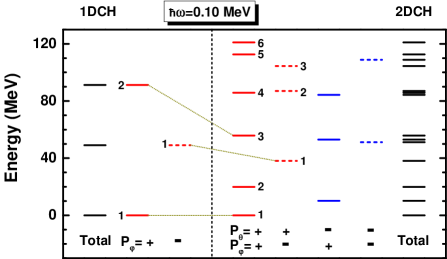
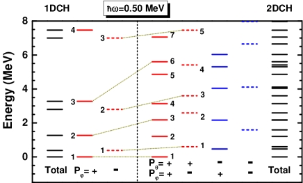
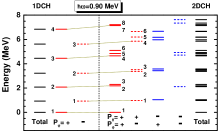
Figure 6: (Color online) Collective energy levels obtained from the two-dimensional collective Hamiltonian in comparison with those from the one-dimensional collective Hamiltonian for $\hbar\omega=0.10$, 0.50, and 0.90 MeV. Note that different scales have been used in different panels.

The comparisons for the collective energy levels at $\hbar\omega=0.10$, 0.50, and 0.90 MeV are shown in Fig. 6. As we have mentioned above, for each cranking frequency, the energy levels of the 2DCH are grouped into $(P_{\theta}P_{\varphi})=(++)$, $(+-)$, $(-+)$, and $(--)$. For the 1DCH, it is invariant with respect to $\varphi\to-\varphi$ and, thus, its solutions can be grouped as $(P_{\varphi})=(+)$ and $(-)$. In Fig. 6, the collective energy levels of the two- and one-dimensional collective Hamiltonians are normalized to the corresponding lowest energy levels $(++)$ and $(+)$, respectively.

Apparently, one obtains more energy levels by solving the 2DCH than solving the 1DCH, since one more degree of freedom $\theta$ has been taken into account. Of course, one cannot find the corresponding energy levels in the groups of $(-+)$ and $(--)$ in the 1DCH results. Only the 2DCH energy levels in the groups of $(++)$ and $(+-)$ with zero-phonon excitation along the $\theta$ direction have their counterparts in the 1DCH. By analyzing the behaviors of the wave functions, one can easily build the connections between the solutions of the one- and two-dimensional Hamiltonians, as shown in Fig. 6 with the dotted lines.

IV.3.2 Wave functions

The comparison of the wave functions can be found in Fig. 7. Here, we take only $\hbar\omega=0.50~{}\rm MeV$ as an example. In order to compare 2DCH wave functions with the 1DCH ones, we chose $\theta=78^{\circ}$ for all the wave functions, and this $\theta$ value is also the position of the minimum in the collective potential (see Fig. 1). In Fig. 7, we present the wave functions of the six lowest energy states in the $(++)$ and $(+-)$ groups of the 2DCH for $\hbar\omega=0.50~{}\rm MeV$, as well as the corresponding wave functions in the 1DCH.

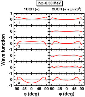
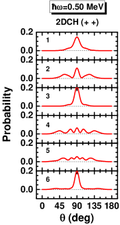
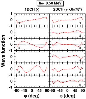
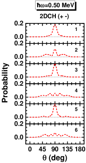
Figure 7: (Color online) Left: The wave functions along the $\varphi$ direction obtained by the 2DCH in comparison with those by the 1DCH. Right: The probability distributions $P(\theta)$ (33) along the $\theta$ direction obtained by the 2DCH.

It can be seen that the behaviors of the wave functions for the 2DCH $(++)$ levels 1, 3, and 6 are similar to those for the one-dimensional $(+)$ levels 1, 2, and 3, respectively. Similar connections can be also found between the two-dimensional $(+-)$ levels 1, 3, and 5, and the one-dimensional $(-)$ levels 1, 2, and 3. This is consistent with the fact that the zero phonon excitation modes along the $\theta$ direction are weakly coupled with the excitations along the $\varphi$ direction.

However, in Fig. 7, no one-dimensional counterpart has been found for the two-dimensional $(++)$ levels 2, 4, and 5, and the $(+-)$ levels 2, 4, and 6. To further examine this point, we also plot the probability distributions of the 2DCH along the $\theta$ direction as shown in Fig. 7. The probability distributions are calculated from the wave functions (28), and the $\varphi$ direction has been integrated by

$$P(\theta)=\int_{-\pi/2}^{\pi/2}|\Psi(\theta,\varphi)|^{2}d\varphi.$$ (33)

Apparently, for each 2DCH level which has an one-dimensional correspondence, i.e., 1, 3, 6 in the $(++)$ group and 1, 3, 5 in the $(+-)$ group, the corresponding probability distribution along the $\theta$ direction has only one peak, and this is associated with a zero-phonon vibration mode along the $\theta$ direction. In contrast, the probability distributions of the other levels have more than one peak, and they correspond to nonzero-phonon vibration mode along the $\theta$ direction. As a result, they have no counterpart in the solutions of the 1DCH. Note that we have also checked the wave functions for other rotational frequencies, and a similar conclusion can be obtained. To avoid repetition, the results are not shown here.

In Fig. 6, we label the counterparts between the 2DCH levels and the 1DCH ones with dashed lines. One can see that, with increasing energy, the energy differences between the 2DCH and 1DCH solutions become larger. This indicates that the one-dimensional approximation is reasonable at low excitation energy. On the other hand, at high rotational frequencies, e.g., $\hbar\omega=0.90~{}\rm MeV$, the 1DCH levels and their 2DCH counterparts are very close to each other. This demonstrates that the one-dimensional approximation may be good at high rotational frequencies, where the rotation mode is close to a principal axis rotation.

IV.4 Excitation modes

In the preceding two sections, the 2DCH collective energy levels and wave functions have been discussed in comparison with the 1DCH ones. As was demonstrated in our previous work Chen et al. (2013), the 1DCH restores the broken chiral symmetry in the aplanar TAC solutions and provides the collective wave functions, which are either symmetric ($P_{\varphi}=+$) or antisymmetric ($P_{\varphi}=-$) with respect to $\varphi\to-\varphi$ transformation. In such a way, it forms pairs of chiral doublet bands along with the increasing rotational frequency. By mapping these one-dimensional solutions to the two-dimensional ones as discussed above (see Figs. 6 and 7), one can certainly expect that the solutions of 2DCH, which have zero-phonon excitation along the $\theta$ direction, can form pairs of chiral doublet bands as well.

Before discussing the other states obtained in the 2DCH, we here recall that the two-dimensional solutions are grouped into four categories with the combination of the symmetries $P_{\theta}$ and $P_{\varphi}$. In fact, the operator $\hat{P}_{\varphi}$ is equivalent to the chiral operator $\hat{\mathcal{T}}\hat{\mathcal{R}}_{2}(\pi)$, while the operator $\hat{P}_{\theta}$ is equivalent to $\hat{\mathcal{T}}\hat{\mathcal{R}}_{3}(\pi)$, or equivalently, the combination of the signature operator $\hat{\mathcal{R}}_{1}(\pi)$ and chiral operators $\hat{P}_{\varphi}$. Here, $\hat{\mathcal{T}}$ and $\hat{\mathcal{R}}_{k}(\pi)$ denote the time-reversal operator and a rotational operator around the $k$ axis by $\pi$, respectively. As the 2DCH is invariant under the $\hat{P}_{\theta}$ and $\hat{P}_{\varphi}$, it is very clear that the broken chiral and signature symmetries in the cranking solutions are both restored in the solutions of 2DCH. In particular, a pair of chiral partner states must be in the groups of $(++)$ and $(+-)$ or of $(-+)$ and $(--)$, differing only in the quantum number associated with $P_{\varphi}$, while a pair of signature partner states must be in the groups of $(++)$ and $(-+)$ or of $(+-)$ and $(--)$ differing only in the quantum number associated with $P_{\theta}$.

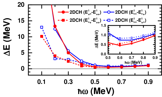
Figure 8: (Color online) The energy splittings between the chiral partner states (open and solid circles) and the signature partner states (open and solid squares) as functions of rotational frequency obtained by 2DCH. Inset: For visibility, the results at the rotational frequency region $0.50\leq\hbar\omega\leq 0.90~{}\rm{MeV}$ are shown at a small scale.

In Fig. 8, the energy splittings between the chiral partner states (open and solid circles), and the signature partner states (open and solid squares) as functions of rotational frequency are shown. Note that we consider here only the lowest level in each group associated with $P_{\theta}$ and $P_{\varphi}$. With the increasing rotational frequency, all the energy splittings show decreasing tendency up to $\hbar\omega\leq 0.60~{}\rm{MeV}$, while they slightly increase at $\hbar\omega>0.60~{}\rm{MeV}$ (see the inset of Fig. 8). The decrease of the energy splittings at $\hbar\omega\leq 0.60~{}\rm{MeV}$ has been discussed in Ref. Chen et al. (2013). They are caused, at low frequencies, mainly by the gradual increase of the mass parameters (see Fig. 2), and at high frequencies, mainly by the appearance of the potential barrier in the collective potentials (see Fig. 1). Note that in this region of rotational frequency, the energy splittings between the signature partners are smaller than those between the chiral partners, and this can be understood from the behaviors of the mass parameters $B_{\theta\theta}$ and $B_{\varphi\varphi}$, as discussed in Sec. IV.2.

The energy splittings increase when $\hbar\omega>0.60~{}\rm{MeV}$, and here the minima of the corresponding TAC solutions are at $(\theta=90^{\circ},\varphi=\pm 90^{\circ})$, which means that the total angular momentum aligns along the intermediate axis, i.e., the axis with the largest moment of inertia. The solutions of 2DCH are mainly from the vibrational motions around the minima $(\theta=90^{\circ},\varphi=\pm 90^{\circ})$ of the TAC solutions. In addition, we note that the angular momenta of the proton and neutron also align along the intermediate axis due to the strong Coriolis interaction. This is reminiscent of the so-called longitudinal wobbling motion Frauendorf and Dönau (2014), in which the wobbling frequency increases with the rotational frequency. Therefore, we clearly provide, in the present framework, a transition from the chiral rotation to the longitudinal wobbling motion.

IV.5 Referring to PRM

For a system with a triaxial rotor coupled to one particle and one hole, its exact solution can be obtained by the diagonalization of the PRM Hamiltonian. Therefore, to examine the quality of the collective Hamiltonian, it is necessary to compare its results with those obtained by the PRM. For the 1DCH, this comparison was made and it was found that not only the yrast band but also the excited partner band in the PRM can be reproduced by the 1DCH Chen et al. (2013). Compared with the 1DCH, the 2DCH further takes the dynamical motion of the $\theta$ degree of freedom into account and, thus, requires again a comparison with the PRM results.

In Fig. 9, the angular momenta of the lowest states in the groups $(++)$, $(+-)$, $(-+)$, and $(--)$ as functions of rotational frequency obtained from the 2DCH are shown in comparison with the yrast and yrare bands (labeled as bands 1 and 2) in the PRM, and the yrast band (labeled as band 1) in the TAC calculations. In the 2DCH, the angular momentum is calculated by considering the fluctuations along the $\theta$ and $\varphi$ directions on top of the TAC solutions:

$$J_{\rm coll}=\int_{0}^{\pi}d\theta\int_{-\pi/2}^{\pi/2}d\varphi\sqrt{w}|\Psi_{\rm coll}(\theta,\varphi)|^{2}J_{\rm TAC}(\theta,\varphi).$$ (34)

Here, $J_{\rm TAC}(\theta,\varphi)$ is the angular momentum calculated by TAC at a given value of $(\theta,\varphi)$, i.e.,

$$J_{\rm TAC}(\theta,\varphi)=\sqrt{J_{1}^{2}(\theta,\varphi)+J_{2}^{2}(\theta,\varphi)+J_{3}^{2}(\theta,\varphi)},$$ (35)

and each component of the angular momentum $J_{k}(\theta,\varphi)$ is the sum of the angular momenta of the particle, the hole, and the rotor at a given $(\theta,\varphi)$:

$$J_{k}(\theta,\varphi) =\langle\psi(\theta,\varphi)|\hat{j}_{k}|\psi(\theta,\varphi)\rangle+R_{k}(\theta,\varphi)$$

$$=\langle\psi(\theta,\varphi)|\hat{j}_{k}|\psi(\theta,\varphi)\rangle+\mathcal{J}_{k}\omega_{k}(\theta,\varphi).$$ (36)

Similar to the TAC calculations, a quantal correction $I_{\rm coll}=J_{\rm coll}-1/2$ Frauendorf (2000) to the angular momentum $J_{\rm coll}$ has also been applied.

Figure 9: (Color online) The angular momenta of the lowest states in groups $(++)$, $(+-)$, $(-+)$, and $(--)$ as functions of rotational frequency obtained from the 2DCH in comparison with the yrast and yrare bands 1 and 2 in the PRM and the yrast band 1 in the TAC. The angular momenta are relative to a rigid-rotor reference $40\omega$.

It is seen that the $I$-$\hbar\omega$ relation in the PRM can be reproduced by both the TAC and the 2DCH. At $\hbar\omega=0.20~{}\rm{MeV}$, a kink appears in the result of the TAC, which is caused by a reorientation of the angular momentum from the 1-3 plane towards to the 2 axis, i.e., from planar to aplanar rotation. In the 2DCH, this kink becomes smooth since the fluctuations around the minima of the collective potential are included. Compared with the TAC solutions, the results obtained from the 2DCH agree slightly better with those of the PRM.

In Fig. 10, we show the calculated energy spectra of these bands. For the TAC calculations, the energy spectra are calculated from the total Routhian as

$$E(I)=E^{\prime}(\omega)+\omega J(\omega).$$ (37)

For the 2DCH, they are calculated with the same method, but the total Routhians are obtained by solving the Hamiltonian in Eq. (5). In the presented results, the energy references of the TAC and the 2DCH are the same.

It has been known that the PRM results show a change of the rotational mode from chiral vibration to chiral rotation, and to wobbling motion at extremely high spins Frauendorf and Meng (1997); Bohr and Mottelson (1975). As mentioned in above discussions (see Sec. IV.2), this feature can be given in the present 2DCH results. Moreover, in the high-spin region, the calculated bands with both the PRM and the 2DCH split into four signature branches, while the TAC solutions cannot provide such splitting. Quantitatively, the 2DCH can reasonably reproduce the PRM results. The favored signature branch of band 1 in the PRM is reproduced by the lowest band in the $(++)$ group of the solutions of the 2DCH. The unfavored signature branch of band 1 and the favored one in band 2 are nearly degenerate in the PRM, and this is well reproduced by the states in the groups of $(+-)$ and $(-+)$ in the 2DCH solutions.

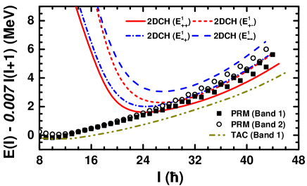
Figure 10: (Color online) The energy spectra of the lowest states in the groups $(++)$, $(+-)$, $(-+)$, and $(--)$ as functions of spin obtained by the 2DCH in comparison with the exact solutions of the PRM, and also the solution of the TAC. The energies are relative to a rigid-rotor reference $0.007I(I+1)$.

In the low-spin region, however, the 2DCH provides decreasing energies with spin up to $I\sim 20\hbar$, and this is inconsistent with the PRM results and also the TAC ones. This may be due to the vibrational frequencies in the mass parameters being neglected in the present calculations; it may not be a good approximation at the low-spin region, because in such cases, the collective potential is harmonic-like with one minimum.

In order to clarify this issue, we include here the vibrational frequencies in our calculations of the mass parameters, but simply by assuming them as constants. The formula of the mass parameter $B_{\varphi\varphi}$ can be found in Eq. (22). For $B_{\theta\theta}$ and $B_{\theta\varphi}$, one can calculate them by

$$B_{\theta\theta} =2\sum_{mi}\frac{(\varepsilon_{m}-\varepsilon_{i})\Big{|}\langle m|\displaystyle\frac{\partial\bm{\omega}}{\partial\theta}\cdot\hat{\bm{j}}|i\rangle\Big{|}^{2}}{[(\varepsilon_{m}-\varepsilon_{i})^{2}-\hbar^{2}\Omega_{\theta}^{2}]^{2}},$$

$$B_{\theta\varphi} =B_{\varphi\theta}=2\sum_{mi}\frac{(\varepsilon_{m}-\varepsilon_{i})\langle m|\displaystyle\frac{\partial\bm{\omega}}{\partial\theta}\cdot\hat{\bm{j}}|i\rangle\langle i|\displaystyle\frac{\partial\bm{\omega}}{\partial\varphi}\cdot\hat{\bm{j}}|m\rangle}{[(\varepsilon_{m}-\varepsilon_{i})^{2}-\hbar^{2}\Omega_{\theta}^{2}][(\varepsilon_{m}-\varepsilon_{i})^{2}-\hbar^{2}\Omega_{\varphi}^{2}]}.$$ (38)

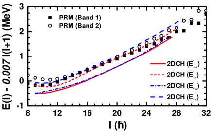
Figure 11: (Color online) Same as Fig. 10, but with the mass parameter calculated by assuming constant vibrational frequencies $\hbar\Omega_{\theta}=\hbar\Omega_{\varphi}=1.10~{}\rm{MeV}$ (see text).

By assuming $\hbar\Omega_{\theta}=\hbar\Omega_{\varphi}=1.10~{}\rm MeV$, in Fig. 11, we show the obtained energy spectra in comparison with the PRM results for the low-spin region. One can see that the energy spectra of the PRM can now be well reproduced. However, a microscopic derivation of these vibrational frequencies $\hbar\Omega_{\theta}$ and $\hbar\Omega_{\varphi}$ is still unresolved, and requires intensive studies in the future.

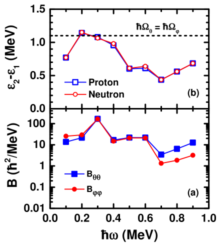
Figure 12: (Color online) The mass parameters $B_{\theta\theta}$ and $B_{\varphi\varphi}$ calculated by Eq. (36) with the vibrational frequencies $\hbar\Omega_{\theta}=\hbar\Omega_{\varphi}=1.10~{}\rm{MeV}$ and the energy differences $\varepsilon_{2}-\varepsilon_{1}$ between the lowest two levels for the proton and neutron obtained by TAC at the minimum of the potential energy surface.

In Fig. 12, we show the mass parameters $B_{\theta\theta}$ and $B_{\varphi\varphi}$ calculated by Eq. (IV.5) with $\hbar\Omega_{\theta}=\hbar\Omega_{\varphi}=1.10~{}\rm MeV$ and the energy differences, $\varepsilon_{2}-\varepsilon_{1}$, between the lowest two levels for the proton and neutron. They are obtained by TAC at the minimum of the potential energy surface. As shown in Fig. 12(b), the energy differences, $\varepsilon_{2}-\varepsilon_{1}$, are high at low $\hbar\omega$, which results in the small mass parameters at low $\hbar\omega$. In Fig. 12(a), with vibrational frequencies $\hbar\Omega_{\theta}=\hbar\Omega_{\varphi}=1.10~{}\rm MeV$ included, the mass parameters are significantly enhanced in low $\hbar\omega$ region and change moderately with $\hbar\omega$ in contrast with the mass parameters calculated with $\hbar\Omega_{\theta}=\hbar\Omega_{\varphi}=0$. This is due to the cancellation between the vibrational frequencies and the energy differences, $\varepsilon_{2}-\varepsilon_{1}$. Therefore the denominators in Eq. (IV.5) are remarkably reduced, which results in the enhanced mass parameters at low $\hbar\omega$. Thus the effects of $\hbar\Omega_{\theta}$ and $\hbar\Omega_{\varphi}$ will reduce the excitation energy and improve the agreement with the results from PRM for lower spins, and maintain the good agreement for higher spins.

V Summary and perspective

In summary, the collective Hamiltonian for chiral and wobbling modes is extended to two dimensions that includes the dynamic motions of both $\theta$ and $\varphi$ and their couplings. Starting from the tilted axis cranking solutions, the collective potential and three mass parameters appearing in the 2DCH are determined on the full $(\theta,\varphi)$ plane. This newly developed model is applied to a triaxial rotor with $\gamma=-30^{\circ}$ coupled with one $h_{11/2}$ proton particle and one $h_{11/2}$ neutron hole.

More excitation modes have been obtained in the 2DCH calculations in comparison with the 1DCH ones. The 2DCH levels, which have the zero-phonon excitation along the $\theta$ direction, have their counterparts in the 1DCH solutions. The 2DCH remains invariant under the chiral and signature operators and, thus, the broken chiral and signature symmetries in the TAC solutions have been restored. As a result, both chiral partners and signature ones can be found in the solutions of the 2DCH. Moreover, the transition from the chiral vibration to the chiral rotation, and to the longitudinal wobbling motion with increasing spin, has been revealed by analyzing the energy splittings of chiral partners and of signature partners in the 2DCH.

The angular momenta and energy spectra calculated by the 2DCH are compared with those by the TAC approach and the exact solutions of PRM. It is demonstrated that the 2DCH can well reproduce the PRM results in the high-spin region by taking the fluctuations along the $\theta$ and $\varphi$ directions into account. However, deviations appear in the low-spin region. By including a constant vibrational frequency in the calculation of the mass parameters, the energy spectra of PRM in the low-spin region can be reproduced.

In the present model, we employed a single-$j$ shell Hamiltonian in the TAC calculations. This is, of course, a rather rough model for describing a realistic nucleus. Therefore, it will be interesting to implement the present collective Hamiltonian on top of a more realistic and microscopic tilted axis cranking theory, e.g., the TAC covariant density functional theory (TAC-CDFT) Madokoro et al. (2000); Peng et al. (2008); Zhao et al. (2011a); Meng et al. (2013); Zhao et al. (2015a); Meng (2016); Meng and Zhao (2016). In particular, the TAC-CDFT has achieved great successes in describing the novel rotational modes, such as the magnetic rotation Zhao et al. (2011a), the antimagnetic rotation Zhao et al. (2011b), and the exotic shape at extreme spin Zhao et al. (2015b). To this end, a three-dimensional axis cranking covariant density functional theory is required. Works along this direction are in progress.

References

- Frauendorf and Meng (1997) S. Frauendorf and J. Meng, Nucl. Phys. A 617, 131 (1997).
- Meng et al. (2008) J. Meng, B. Qi, S. Q. Zhang, and S. Y. Wang, Mod. Phys. Lett. A 23, 2560 (2008).
- Meng and Zhang (2010) J. Meng and S. Q. Zhang, J. Phys. G: Nucl. Part. Phys. 37, 064025 (2010).
- Meng et al. (2014) J. Meng, Q. B. Chen, and S. Q. Zhang, Int. J. Mod. Phys. E 23, 1430016 (2014).
- Bark et al. (2014) R. A. Bark, E. O. Lieder, R. M. Lieder, E. A. Lawrie, J. J. Lawrie, S. P. Bvumbi, N. Y. Kheswa, S. S. Ntshangase, T. E. Madiba, P. L. Masiteng, et al., Int. J. Mod. Phys. E 23, 1461001 (2014).
- Bohr and Mottelson (1975) A. Bohr and B. R. Mottelson, Nuclear structure, vol. II (Benjamin, New York, 1975).
- Odegaard et al. (2001) S. W. Odegaard, G. B. Hagemann, D. R. Jensen, M. Bergström, B. Herskind, G. Sletten, S. Törmänen, J. N. Wilson, P. O. Tjøm, I. Hamamoto, et al., Phys. Rev. Lett. 86, 5866 (2001).
- Amro et al. (2003) H. Amro, W. C. Ma, G. B. Hagemann, R. M. Diamond, J. Domscheit, P. Fallon, A. Gorgen, B. Herskind, H. Hubel, D. R. Jensen, et al., Phys. Lett. B 553, 197 (2003).
- Schönwaßer et al. (2003) G. Schönwaßer, H. Hübel, G. B. Hagemann, P. Bednarczyk, G. Benzoni, A. Bracco, P. Bringel, R. Chapman, D. Curien, J. Domscheit, et al., Phys. Lett. B 552, 9 (2003).
- Bringel et al. (2005) P. Bringel, G. B. Hagemann, H. Hübel, A. Al-khatib, P. Bednarczyk, A. Bürger, D. Curien, G. Gangopadhyay, B. Herskind, D. R. Jensen, et al., Eur. Phys. J. A 24, 167 (2005).
- Hartley et al. (2009) D. J. Hartley, R. V. F. Janssens, L. L. Riedinger, M. A. Riley, A. Aguilar, M. P. Carpenter, C. J. Chiara, P. Chowdhury, I. G. Darby, U. Garg, et al., Phys. Rev. C 80, 041304 (2009).
- Matta et al. (2015) J. T. Matta, U. Garg, W. Li, S. Frauendorf, A. D. Ayangeakaa, D. Patel, K. W. Schlax, R. Palit, S. Saha, J. Sethi, et al., Phys. Rev. Lett. 114, 082501 (2015).
- Peng et al. (2003) J. Peng, J. Meng, and S. Q. Zhang, Phys. Rev. C 68, 044324 (2003).
- Koike et al. (2004) T. Koike, K. Starosta, and I. Hamamoto, Phys. Rev. Lett. 93, 172502 (2004).
- Zhang et al. (2007) S. Q. Zhang, B. Qi, S. Y. Wang, and J. Meng, Phys. Rev. C 75, 044307 (2007).
- Higashiyama and Yoshinaga (2007) K. Higashiyama and N. Yoshinaga, Eur. Phys. J. A 33, 355 (2007).
- Qi et al. (2009) B. Qi, S. Q. Zhang, J. Meng, S. Y. Wang, and S. Frauendorf, Phys. Lett. B 675, 175 (2009).
- Chen et al. (2010) Q. B. Chen, J. M. Yao, S. Q. Zhang, and B. Qi, Phys. Rev. C 82, 067302 (2010).
- Lawrie and Shirinda (2010) E. A. Lawrie and O. Shirinda, Phys. Lett. B 689, 66 (2010).
- Rohozinski et al. (2011) S. G. Rohozinski, L. Prochniak, K. Starosta, and C. Droste, Eur. Phys. J. A 47, 90 (2011).
- Shirinda and Lawrie (2012) O. Shirinda and E. A. Lawrie, Eur. Phys. J. A 48, 118 (2012).
- Zhang and Chen (2016) H. Zhang and Q. B. Chen, Chin. Phys. C 40, 024101 (2016).
- Hamamoto (2002) I. Hamamoto, Phys. Rev. C 65, 044305 (2002).
- Hamamoto and Mottelson (2003) I. Hamamoto and B. R. Mottelson, Phys. Rev. C 68, 034312 (2003).
- Frauendorf and Dönau (2014) S. Frauendorf and F. Dönau, Phys. Rev. C 89, 014322 (2014).
- Shi and Chen (2015) W. X. Shi and Q. B. Chen, Chin. Phys. C 39, 054105 (2015).
- Dimitrov et al. (2000) V. I. Dimitrov, S. Frauendorf, and F. Dönau, Phys. Rev. Lett. 84, 5732 (2000).
- Olbratowski et al. (2004) P. Olbratowski, J. Dobaczewski, J. Dudek, and W. Płóciennik, Phys. Rev. Lett. 93, 052501 (2004).
- Olbratowski et al. (2006) P. Olbratowski, J. Dobaczewski, and J. Dudek, Phys. Rev. C 73, 054308 (2006).
- Mukhopadhyay et al. (2007) S. Mukhopadhyay, D. Almehed, U. Garg, S. Frauendorf, T. Li, P. V. M. Rao, X. Wang, S. S. Ghugre, M. P. Carpenter, S. Gros, et al., Phys. Rev. Lett. 99, 172501 (2007).
- Almehed et al. (2011) D. Almehed, F. Dönau, and S. Frauendorf, Phys. Rev. C 83, 054308 (2011).
- Shimizu and Matsuzaki (1995) Y. R. Shimizu and M. Matsuzaki, Nucl. Phys. A 588, 559 (1995).
- Matsuzaki et al. (2002) M. Matsuzaki, Y. R. Shimizu, and K. Matsuyanagi, Phys. Rev. C 65, 041303 (2002).
- Matsuzaki et al. (2004a) M. Matsuzaki, Y. R. Shimizu, and K. Matsuyanagi, Eur. Phys. J. A 20, 189 (2004a).
- Matsuzaki et al. (2004b) M. Matsuzaki, Y. R. Shimizu, and K. Matsuyanagi, Phys. Rev. C 69, 034325 (2004b).
- Matsuzaki and Ohtsubo (2004) M. Matsuzaki and S. Ohtsubo, Phys. Rev. C 69, 064317 (2004).
- Shimizu et al. (2005) Y. R. Shimizu, M. Matsuzaki, and K. Matsuyanagi, Phys. Rev. C 72, 014306 (2005).
- Shimizu et al. (2008) Y. R. Shimizu, T. Shoji, and M. Matsuzaki, Phys. Rev. C 77, 024319 (2008).
- Shoji and Shimizu (2009) T. Shoji and Y. R. Shimizu, Progr. Theor. Phys. 121, 319 (2009).
- Frauendorf and Dönau (2015) S. Frauendorf and F. Dönau, Phys. Rev. C 92, 064306 (2015).
- Brant et al. (2004) S. Brant, D. Vretenar, and A. Ventura, Phys. Rev. C 69, 017304 (2004).
- Higashiyama et al. (2005) K. Higashiyama, N. Yoshinaga, and K. Tanabe, Phys. Rev. C 72, 024315 (2005).
- Bhat et al. (2014) G. H. Bhat, J. A. Sheikh, W. A. Dar, S. Jehangir, R. Palit, and P. A. Ganai, Phys. Lett. B 738, 218 (2014).
- Chen et al. (2013) Q. B. Chen, S. Q. Zhang, P. W. Zhao, R. V. Jolos, and J. Meng, Phys. Rev. C 87, 024314 (2013).
- Chen (2015) Q. B. Chen, Acta Phys. Pol. B Proc. Suppl. 8, 545 (2015).
- Chen et al. (2014) Q. B. Chen, S. Q. Zhang, P. W. Zhao, and J. Meng, Phys. Rev. C 90, 044306 (2014).
- Ring and Schuck (1980) P. Ring and P. Schuck, The nuclear many body problem (Springer Verlag, Berlin, 1980).
- Baranger and Kumar (1968) M. Baranger and K. Kumar, Nucl. Phys. A 122, 241 (1968).
- Matsuo et al. (2000) M. Matsuo, T. Nakatsukasa, and K. Matsuyanagi, Prog. Theor. Phys. 103, 959 (2000).
- Matsuyanagi et al. (2010) K. Matsuyanagi, M. Matsuo, T. Nakatsukasa, N. Hinohara, and K. Sato, J. Phys. G: Nucl. Part. Phys. 37, 064018 (2010).
- Marumori et al. (1980) T. Marumori, T. Maskawa, F. Sakata, and A. Kuriyama, Prog. Theor. Phys. 64, 1294 (1980).
- Pauli (1933) W. Pauli, in Handbuch der Physik, vol. XXIV, p. 120 (Springer Verlag, Berlin, 1933).
- Frauendorf and Meng (1996) S. Frauendorf and J. Meng, Z. Phys. A 356, 263 (1996).
- Frauendorf (2000) S. Frauendorf, Nucl. Phys. A 677, 115 (2000).
- Madokoro et al. (2000) H. Madokoro, J. Meng, M. Matsuzaki, and S. Yamaji, Phys. Rev. C 62, 061301 (2000).
- Peng et al. (2008) J. Peng, J. Meng, P. Ring, and S. Q. Zhang, Phys. Rev. C 78, 024313 (2008).
- Zhao et al. (2011a) P. W. Zhao, S. Q. Zhang, J. Peng, H. Z. Liang, P. Ring, and J. Meng, Phys. Lett. B 699, 181 (2011a).
- Meng et al. (2013) J. Meng, J. Peng, S. Q. Zhang, and P. W. Zhao, Front. Phys. 8, 55 (2013).
- Zhao et al. (2015a) P. W. Zhao, S. Q. Zhang, and J. Meng, Phys. Rev. C 92, 034319 (2015a).
- Meng (2016) J. Meng, ed., Relativistic density functional for nuclear structure (World Scientific, Singapore, 2016).
- Meng and Zhao (2016) J. Meng and P. W. Zhao, Phys. Scr. 91, 053008 (2016).
- Zhao et al. (2011b) P. W. Zhao, J. Peng, H. Z. Liang, P. Ring, and J. Meng, Phys. Rev. Lett. 107, 122501 (2011b).
- Zhao et al. (2015b) P. W. Zhao, N. Itagaki, and J. Meng, Phys. Rev. Lett. 115, 022501 (2015b).