Quantum Tunneling In Deformed Quantum Mechanics with Minimal Length

Abstract

In the deformed quantum mechanics with a minimal length, one WKB connection formula through a turning point is derived. We then use it to calculate tunnelling rates through potential barriers under the WKB approximation. Finally, the minimal length effects on two examples of quantum tunneling in nuclear and atomic physics are discussed.

I Introduction

Various theories of quantum gravity, such as string theory, loop quantum gravity and quantum geometry, predict the existence of a minimal length IN-Townsend:1977xw ; IN-Amati:1988tn ; IN-Konishi:1989wk . For a review of a minimal length in quantum gravity, see IN-Garay:1994en . Some realizations of the minimal length from various scenarios have been proposed. Specifically, one of the most popular models is the Generalized Uncertainty Principle (GUP) IN-Maggiore:1993kv ; IN-Kempf:1994su , derived from the modified fundamental commutation relation:

$$[X,P]=i\hbar(1+\beta P^{2}),$$ (1)

where $\beta=\beta_{0}\ell_{p}^{2}/\hbar^{2}=\beta_{0}/c^{2}m_{pl}^{2}$, $m_{pl}$ is the Planck mass, $\ell_{p}$ is the Planck length, and $\beta_{0}$ is a dimensionless parameter. With this modified commutation relation, one can easily find

$$\Delta X\Delta P\geq\frac{\hbar}{2}[1+\beta(\Delta P)^{2}],$$ (2)

which leads to the minimal measurable length:

$$\Delta X\geq\Delta_{\text{min}}=\hbar\sqrt{\beta}=\sqrt{\beta_{0}}\ell_{p}.$$ (3)

The GUP has been extensively studied recently, see for example IN-Chang:2001bm ; IN-Brau:1999uv ; IN-Das:2008kaa ; IN-Hossenfelder:2003jz ; IN-Ali:2009zq ; IN-Li:2002xb ; IN-Brau:2006ca ; IN-Wang:2015bwa . For a review of the GUP, see IN-Hossenfelder:2012jw .

To study 1D quantum mechanics with the deformed commutators $(\ref{1dGUP})$, one can exploit the following representation for $X$ and $P$:

$$X=X_{0}\text{, }P=P_{0}\left(1+\frac{\beta}{3}P_{0}^{2}\right),$$ (4)

where $[X_{0},P_{0}]=i\hbar$. It can easily show that such representation fulfills the relation $(\ref{1dGUP})$ to $\mathcal{O}\left(\beta\right)$. Furthermore, we can adopt the position representation:

$$X_{0}=x\text{, }P_{0}=\frac{\hbar}{i}\frac{\partial}{\partial x}\text{.}$$ (5)

Therefore for a quantum system described by

$$H=\frac{P^{2}}{2m}+V\left(X\right),$$ (6)

the deformed stationary Schrodinger equation in the position representation is

$$\frac{d^{2}\psi\left(x\right)}{dx^{2}}-\ell_{\beta}^{2}\frac{d^{4}\psi\left(x\right)}{dx^{4}}+\frac{2m\left[E-V\left(x\right)\right]}{\hbar^{2}}\psi\left(x\right)=0.$$ (7)

where $\ell_{\beta}^{2}\equiv\frac{2}{3}\hbar^{2}\beta$ and terms of order $\beta^{2}$ are neglected.

If eqn. $\left(\ref{eq: Sch-eqn}\right)$ with $\beta=0$ can be solved exactly, one could use the perturbation method to solve eqn. $\left(\ref{eq: Sch-eqn}\right)$ by treating the term with $\ell_{\beta}^{2}$ as a small correction. However for the general $V\left(x\right)$, one might need other methods to solve eqn. $\left(\ref{eq: Sch-eqn}\right)$. In fact, the WKB approximation in deformed space have been considered IN-Fityo:2005lwa . In IN-Fityo:2005lwa , the authors considered the deformed commutation relation

$$\left[X,P\right]=i\hbar f\left(P\right),$$ (8)

where $f\left(P\right)$ is some function. For $f\left(P\right)$, one could solve the differential equation

$$\frac{dP\left(p\right)}{dp}=f\left(P\right)$$ (9)

for $P\left(p\right)$, and $p\left(P\right)$ denotes the inverse function of $P\left(p\right)$. It is interesting to note that there might be more than one inverse function for $P\left(p\right)$. However, one usually finds that there is only one inverse function $p\left(P\right)$ which vanishes at $P=0$. The rest ones are called ”runaway” solutions, which are not physical and should be discarded IN-Simon:1990ic ; IN-Mu:2015qna . Then, they used the WKB approximation to show that the solution to the deformed Schrodinger equation:

$$P^{2}\left(\frac{\hbar}{i}\frac{d}{dx}\right)\psi\left(x\right)+2m\left[V\left(x\right)-E\right]\psi\left(x\right)=0,$$ (10)

was

$$\psi\left(x\right)=\frac{1}{\sqrt{\left|P\left(x\right)f\left(P\left(x\right)\right)\right|}}\left(C_{1}\exp\left[\frac{i}{\hbar}\int^{x}p\left(P\left(x\right)\right)dx\right]+C_{2}\exp\left[-\frac{i}{\hbar}\int^{x}p\left(P\left(x\right)\right)dx\right]\right),$$ (11)

where $P\left(x\right)=\sqrt{2m\left[E-V\left(x\right)\right]}$. Moreover, it also showed that the condition

$$\left|P^{2}\left(x\right)\right|\gg\hbar\left|\frac{d}{dx}P\left(x\right)f\left(P\left(x\right)\right)\right|,$$ (12)

had to be satisfied to make the WKB approximation valid. However, the condition $\left(\ref{eq:Condition}\right)$ fails near a turning point where $P\left(x\right)=0$.

For the case with $f\left(P\right)=1+\beta P^{2}$, we derived one WKB connection formula through turning points and Bohr-Sommerfeld quantization rule in IN-Tao:2012fp . In this paper, we continue to consider other WKB connection formulas and calculate tunnelling rates through potential barriers. The remainder of our paper is organized as follows. In section II, we derive one WKB connection formula and use it to find the formula for the tunnelling rate through a potential barrier. Then two examples of quantum tunneling in nuclear and atomic physics are discussed in section III. Section IV is devoted to our conclusions.

II Tunneling Through Potential Barriers

We now consider WKB description of tunneling through a potential barrier $V\left(x\right)$, which vanishes as $x\rightarrow\pm\infty$ and rises monotonically to its maximum $V_{\max}$ at $x=x_{0}$ as $x$ approaches $x_{0}$ from either the left or the right side of $x_{0}$. In FIG. 1, we plot the potential $V\left(x\right)$. For a particle of energy $E$, there are two turning points $x=x_{1}\$and $x=x_{2}$, $x_{1}<x_{2}$, at which $V\left(x\right)=E$. There are two classical allowed regions, Region I with $x<x_{1}$ and Region III with $x>x_{2}$. To describe tunneling, we need to choose appropriate boundary conditions in the classical allowed regions. We postulate an incident right-moving wave in Region I, where the WKB approximation solution to eqn. $\left(\ref{eq:deformed-Sch-general}\right)$ includes a wave incident the barrier and a reflected wave:

$$\psi\left(x\right)=\frac{A\exp\left[-\frac{i}{\hbar}\int_{x}^{x_{1}}p\left(P\left(x\right)\right)dx\right]}{\sqrt{\left|P\left(x\right)f\left(P\left(x\right)\right)\right|}}+\frac{B\exp\left[\frac{i}{\hbar}\int_{x}^{x_{1}}p\left(P\left(x\right)\right)dx\right]}{\sqrt{\left|P\left(x\right)f\left(P\left(x\right)\right)\right|}}.$$ (13)

In Region III, there is only a transmitted wave:

$$\psi\left(x\right)=\frac{F\exp\left[\frac{i}{\hbar}\int_{x_{2}}^{x}p\left(P\left(x\right)\right)dx\right]}{\sqrt{\left|P\left(x\right)f\left(P\left(x\right)\right)\right|}}.$$ (14)

In the classically forbidden Region II, there are exponentially growing and decaying solutions:

$$\psi\left(x\right) =\frac{C\exp\left[-\frac{1}{\hbar}\int_{x_{1}}^{x}\left|p\left(P\left(x\right)\right)\right|dx\right]}{\sqrt{\left|P\left(x\right)f\left(P\left(x\right)\right)\right|}}+\frac{D\exp\left[\frac{1}{\hbar}\int_{x_{1}}^{x}\left|p\left(P\left(x\right)\right)\right|dx\right]}{\sqrt{\left|P\left(x\right)f\left(P\left(x\right)\right)\right|}}$$

$$=\frac{C^{\prime}\exp\left[\frac{1}{\hbar}\int_{x}^{x_{2}}\left|p\left(P\left(x\right)\right)\right|dx\right]}{\sqrt{\left|P\left(x\right)f\left(P\left(x\right)\right)\right|}}+\frac{D^{\prime}\exp\left[-\frac{1}{\hbar}\int_{x}^{x_{2}}\left|p\left(P\left(x\right)\right)\right|dx\right]}{\sqrt{\left|P\left(x\right)f\left(P\left(x\right)\right)\right|}},$$ (15)

where

$$C^{\prime} =Ce^{-\eta},D^{\prime}=De^{\eta},$$

$$\eta \equiv\frac{1}{\hbar}\int_{x_{1}}^{x_{2}}\left|p\left(P\left(x\right)\right)\right|dx.$$ (16)

To calculate the tunneling rate, we need to use connection formulas to relate $F$, $C/C^{\prime}$, and $D/D^{\prime}$ to $A$. In IN-Tao:2012fp , we derived one WKB connection formula around $x=x_{1}$ in the case with $f\left(P\right)=1+\beta P^{2}$. If $D=0$, we found that

$$\frac{C}{\sqrt{\left|P\left(x\right)f\left(P\left(x\right)\right)\right|}}\exp\left(-\frac{1}{\hbar}\int_{x_{1}}^{x}\left|p\left(P\left(x\right)\right)\right|dx\right)$$

$$\rightarrow\frac{2C}{\sqrt{\left|P\left(x\right)f\left(P\left(x\right)\right)\right|}}\sin\left(\frac{1}{\hbar}\int_{x_{1}}^{x}p\left(P\left(x\right)\right)dx+\frac{\pi}{4}\right)\text{, to }\mathcal{O}\left(\beta^{2}\right),$$ (17)

which gives

$$A=Ce^{-\frac{i\pi}{4}}.$$ (18)

In what follows, we will derive a WKB connection formula around $x=x_{2}$ to relate $C^{\prime}$ and $D^{\prime}$ to $F$ and then calculate the tunneling rate through the potential barrier.

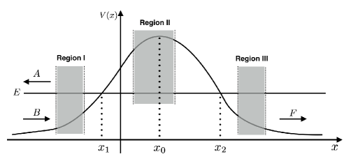
Figure 1: Scattering from a potential barrier.

To match WKB solutions, we need to solve the deformed Schrodinger equation $\left(\ref{eq: Sch-eqn}\right)$ in the vicinity of the turning point $x=x_{2}$. A linear approximation to the potential $V\left(x\right)$ near the turning point $x=x_{2}$ is

$$V\left(x\right)\approx V\left(x_{2}\right)-\left|V^{\prime}\left(x_{2}\right)\right|\left(x-x_{2}\right),$$ (19)

where $V\left(x_{2}\right)=E$. To simplify eqn. $\left(\ref{eq: Sch-eqn}\right)$, a new dimensionless variable $\rho$ could be introduced:

$$\rho=\left(x_{2}-x\right)\left(2m\left|V^{\prime}\left(x_{2}\right)\right|/\hbar^{2}\right)^{\frac{1}{3}}.$$ (20)

Thus, eqn. $\left(\ref{eq: Sch-eqn}\right)$ becomes

$$-\alpha^{2}\frac{d^{4}\psi\left(\rho\right)}{d\rho^{4}}+\frac{d^{2}\psi\left(\rho\right)}{d\rho^{2}}-\rho\psi\left(\rho\right)=0,$$ (21)

where $\alpha^{2}=\left(2m\left|V^{\prime}\left(x_{2}\right)\right|/\hbar^{2}\right)^{\frac{2}{3}}\ell_{\beta}^{2}$. The differential equation $\left(\ref{eq: Sch-eqn}\right)$ can be solved by Laplace’s method IN-Tao:2012fp . Integral representations of the solutions are

$$I\left(\rho\right)=\int_{C}\exp\left(\rho t+\frac{\alpha^{2}t^{5}}{5}-\frac{t^{3}}{3}\right)dt,$$ (22)

where the contour $C$ is chosen so that the integrand vanishes at endpoints of $C$. Specifically, define five sectors:

$$\Theta_{n}\equiv\left[\frac{2n\pi+\frac{\pi}{2}}{5},\frac{2n\pi+\frac{3\pi}{2}}{5}\right],\text{ }n=0,1,2,3,4.$$ (23)

The contour $C$ must originate at one of them and terminate at another.

The asymptotic expressions of $I\left(\rho\right)$ for large values of $\rho$ can be obtained by evaluating the integral $\left(\ref{eq:solution}\right)$ using the method of steepest descent. To do this, we make the change of variables $t=\left|\rho\right|^{\frac{1}{2}}s$ and find

$$I\left(\rho\right)=\left|\rho\right|^{\frac{1}{2}}\int_{C}\exp\left[\left|\rho\right|^{\frac{3}{2}}f_{\pm}\left(s\right)\right]ds,$$ (24)

where $f_{\pm}\left(s\right)$ $\equiv\pm s-\frac{s^{3}}{3}+\frac{as^{5}}{5}$ with $+$ for $\rho>0$ and $-$ for $\rho<0$, and $a\equiv\alpha^{2}\left|\rho\right|\ll 1$ in the physical region IN-Tao:2012fp . We will show below that there exists a steepest descent contour ranging from $s=\infty\exp\left(\frac{7\pi i}{5}\right)$ to $s=\infty\exp\left(\frac{9\pi i}{5}\right)$, which is the red contour in FIG. 3. Such contour could let us match the asymptotic expression of $I\left(\rho\right)$ at large negative value of $\rho$ with the WKB solution $\left(\ref{eq:Trans-WKB}\right)$ in Region III. Note that $\infty\exp\left(\frac{7\pi i}{5}\right)\in\Theta_{3}$ and $\infty\exp\left(\frac{7\pi i}{5}\right)\in\Theta_{4}$.

The method of steepest descent is very powerful to calculate integrals of the form

$$I\left(x\right)=\int_{C}g\left(z\right)e^{xf\left(z\right)}dz,$$ (25)

where $C$ is a contour in the complex plane. We are usually interested in the behavior of $I\left(x\right)$ as $x\rightarrow\infty$. The key step of the method of steepest descent is applying Cauchy’s theorem to deform the contours $C$ to the contours coinciding with steepest descent paths. Around a saddle point $z_{0}$ where $f^{\prime}\left(z_{0}\right)=0$, there are two cosntant-phase (steepest) contours, on which $\operatorname{Im}f\left(z\right)$ is constant, passing through $z_{0}$ if $f^{\prime\prime}\left(z_{0}\right)\neq 0$. One of them is a steepest descent contour, along which $\operatorname{Re}f\left(z\right)$ increases as we go towards $z_{0}$. The other is a steepest ascent contour, along which $\operatorname{Re}f\left(z\right)$ decreases as we go towards $z_{0}$. If $I\left(x\right)$ is integrated along the steepest descent contour, the asymptotic behavior of $I\left(x\right)$ is dominated by the contribution from the saddle point $z_{0}$.

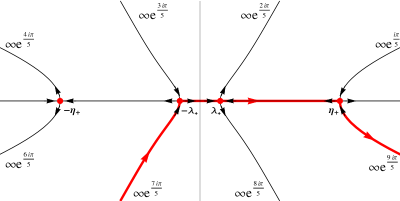
Figure 2: Saddle points and cosntant-phase (steepest) contours of $f_{+}\left(s\right)$. The red contour is a steepest descent contour, along which $I\left(\rho\right)$ is integrated. The black arrows on the cosntant-phase contours around saddle points denote the directions in which values of $\operatorname{Re}f_{+}\left(s\right)$ increase.

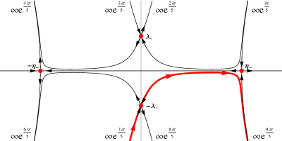
Figure 3: Saddle points and cosntant-phase (steepest) contours of $f_{-}\left(s\right)$. The red contour is a steepest descent contour, along which $I\left(\rho\right)$ is integrated. The black arrows on the cosntant-phase contours around saddle points denote the directions in which values of $\operatorname{Re}f_{-}\left(s\right)$ increase.

In FIGs. 2 and 3, we plot saddle points (red points in figures) of $f_{+}\left(s\right)$ and $f_{-}\left(s\right)$, respectively, and cosntant-phase contours passing through them. Specifically, saddle points of $f_{+}\left(s\right)$ are

$$s=\pm\lambda_{+}\equiv\pm\frac{\sqrt{1-\sqrt{1-4a}}}{\sqrt{2a}}\text{ and }s=\pm\eta_{+}\equiv\pm\frac{\sqrt{1+\sqrt{1-4a}}}{\sqrt{2a}},$$ (26)

and these of $f_{-}\left(s\right)$ are

$$s=\pm\lambda_{-}\equiv\pm\frac{\sqrt{1-\sqrt{1+4a}}}{\sqrt{2a}}\text{ and }s=\pm\eta_{-}\equiv\pm\frac{\sqrt{1+\sqrt{1+4a}}}{\sqrt{2a}}.$$ (27)

The red contours in FIGs. 2 and 3 are the steepest descent contours connecting $s=\infty\exp\left(\frac{7\pi i}{5}\right)$ to $s=\infty\exp\left(\frac{9\pi i}{5}\right)$, along which the integral $\left(\ref{eq:int-rho}\right)$ is integrated. Note that red arrows on them denote the steepest contours’ directions. On the other hand, the black arrows on the cosntant-phase contours around saddle points denote the directions in which values of $\operatorname{Re}f_{\pm}\left(s\right)$ increase. Following the black arrows on the red contour in FIG. 2, we find that $\operatorname{Re}f_{+}\left(-\lambda_{+}\right)$ and $\operatorname{Re}f_{+}\left(\eta_{+}\right)$ are smaller than $\operatorname{Re}f_{+}\left(\lambda_{+}\right)$. Thus for the case with $\rho>0$, the asymptotic expression of $I\left(\rho\right)$ is dominated by the contribution from the saddle $s=\lambda_{+}$. The method of steepest descent gives

$$I\left(1\ll\rho\ll\alpha^{-2}\right) \sim\frac{\sqrt{\pi}\exp\left[\rho^{\frac{3}{2}}f_{+}\left(\lambda_{+}\right)\right]}{\rho^{\frac{1}{4}}}\sqrt{\frac{2}{\left|f_{+}^{\prime\prime}\left(\lambda_{+}\right)\right|}}$$

$$\sim\frac{\sqrt{\pi}\left(1+\frac{3}{4}a\right)}{\rho^{\frac{1}{4}}}\exp\left[\frac{2\rho^{\frac{3}{2}}}{3}\left(1+\frac{3a}{10}\right)\right],$$ (28)

where $a\ll 1$ is used, and terms of $\mathcal{O}\left(a^{2}\right)$ are neglected in the second line. For the case with $\rho>0$, FIG. 3 shows that the asymptotic expression of $I\left(\rho\right)$ is dominated by the contribution from the saddle $s=-\lambda_{-}$, and hence we find

$$I\left(-1\gg\rho\gg-\alpha^{-2}\right) \sim\frac{\sqrt{\pi}\exp\left(\frac{\pi}{4}i\right)\exp\left[\left|\rho\right|^{\frac{3}{2}}f_{-}\left(-\lambda_{-}\right)\right]}{\left|\rho\right|^{\frac{1}{4}}}\sqrt{\frac{2}{\left|f_{-}^{\prime\prime}\left(-\lambda_{+}\right)\right|}}$$

$$\sim\frac{\sqrt{\pi}\exp\left(\frac{\pi}{4}i\right)\left(1-\frac{3}{4}a\right)}{\left|\rho\right|^{\frac{1}{4}}}\exp\left[\frac{2i\left|\rho\right|^{\frac{3}{2}}}{3}\left(1-\frac{3a}{10}\right)\right],$$ (29)

where terms of $\mathcal{O}\left(a^{2}\right)$ are neglected in the second line.

Around the turning point $x=x_{2}$, $\left|x-x_{2}\right|\ll 1$ and $P\left(x\right)\sim\sqrt{2m\left|V^{\prime}\left(x_{2}\right)\right|}\sqrt{x-x_{2}}$. In this region, we find that WKB solutions $\left(\ref{eq:Trans-WKB}\right)$ and $\left(\ref{eq:Forb-WKB}\right)$ become

$$\psi\left(x\right) \sim\frac{F}{\left(2m\left|V^{\prime}\left(x_{2}\right)\right|/\hbar^{2}\right)^{\frac{1}{3}}\hbar}\frac{1-\frac{3a}{4}}{\left|\rho\right|^{\frac{1}{4}}}\exp\left[\frac{2i\left|\rho\right|^{\frac{3}{2}}}{3}\left(1-\frac{3a}{10}\right)\right],$$

$$\psi\left(x\right) \sim\frac{1}{\left(2m\left|V^{\prime}\left(x_{2}\right)\right|/\hbar^{2}\right)^{\frac{1}{3}}\hbar}\frac{1+\frac{3}{4}a}{\rho^{\frac{1}{4}}}\left\{C^{\prime}\exp\left[\frac{2\rho^{\frac{3}{2}}}{3}\left(1+\frac{3a}{10}\right)\right]+D^{\prime}\exp\left[-\frac{2\rho^{\frac{3}{2}}}{3}\left(1+\frac{3a}{10}\right)\right]\right\},$$ (30)

where we use $p\left(P\right)\approx P-\frac{\beta}{3}P^{3}$ and terms of $\mathcal{O}\left(a^{2}\right)$ are neglected, and we express $x$ in terms of $\rho$ using eqn. $\left(\ref{eq:rho-x}\right)$. In the overlap regions where $\left|\rho\right|\gg 1$ and $\left|x-x_{2}\right|\ll 1$, matching WKB solutions $\left(\ref{eq:WKB-Aprro}\right)$ with the $I\left(\rho\right)$’s asymptotic expressions $\left(\ref{eq:I-largeP-rho}\right)$ and $\left(\ref{eq:I-largeN-rho}\right)$ gives

$$C^{\prime}=F\exp\left(-\frac{\pi}{4}i\right)\text{ and }D^{\prime}=0\text{,}$$ (31)

which by eqns. $\left(\ref{eq:CD-CDprime}\right)$ lead to $C=F\exp\left(-\frac{\pi}{4}i\right)e^{\eta}$ and $D=0$. Since $D=0$, eqn. $\left(\ref{eq:A-C}\right)$ gives

$$F=iAe^{-\eta},$$ (32)

and the transmission probability is

$$T=\frac{\left|F\right|^{2}}{\left|A\right|^{2}}\sim e^{-2\eta}.$$ (33)

III Examples

The dimensionless number $\beta_{0}=c^{2}m_{pl}^{2}\beta=\hbar^{2}\beta/\ell_{p}^{2}$ plays an important role when implications and applications of non-zero minimal length are discussed. Normally, if the minimal length is assumed to be order of the Planck length $\ell_{p}$, one has $\beta_{0}\sim 1$. In IN-Das:2008kaa , based on the precision measurement of STM current, an upper bound of $\beta_{0}$ was given by $\beta_{0}<10^{21}$. In the following, we use eqn. $\left(\ref{eq:tunneling}\right)$ to study effects of GUP on $\alpha$ decay and cold electrons emission from metal via strong external electric field.

III.1 $\alpha$ Decay

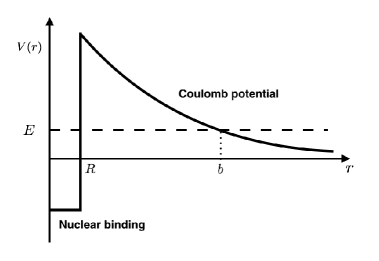
Figure 4: The potential energy of an $\alpha$-particle in a radioactive nucleus.

The decay of a nucleus into an $\alpha$-particle (charge $2e$) and a daughter nucleus (charge $Ze$) can be described as the tunneling of an $\alpha$-particle through a barrier caused by the Coulomb potential between the daughter and the $\alpha$-particle (FIG. 4) APP-Gamow:1928zz . For an $\alpha$-particle of energy $E$ in the potential in FIG. 4, there are two turning points, the nuclear radius $R$ and the outer turning point $b$, which is determined by

$$E=\frac{Ze^{2}}{2\pi\varepsilon_{0}r}\Rightarrow b=\frac{Ze^{2}}{2\pi\varepsilon_{0}E}.$$ (34)

The exponent $\eta$ in eqn. $\left(\ref{eq:tunneling}\right)$ is

$$\eta =\frac{1}{\hbar}\int_{R}^{b}\left|p\left(\sqrt{2mE}\sqrt{1-\frac{Z_{1}Z_{2}e^{2}}{4\pi\varepsilon_{0}Er}}\right)\right|dx$$

$$\approx\frac{\sqrt{2mE}}{\hbar}\left\{b\arccos\left(\sqrt{\frac{R}{b}}\right)-\sqrt{R\left(b-R\right)}\right.$$

$$\left.+\frac{2mE\beta}{3}\left[3b\operatorname{arcsec}\sqrt{\frac{b}{R}}-\sqrt{R\left(b-R\right)}-2b\sqrt{\frac{b-R}{R}}\right]\right\},$$ (35)

where $m$ is the mass of the $\alpha$-particle. At low energies (relative to the height of the Coulomb barrier at $r=R$), we have $b\gg R$ and then

$$\eta\approx\frac{\sqrt{2m}e^{2}}{4\varepsilon_{0}\hbar}\left[1-\frac{8mE\beta}{3\pi}\sqrt{\frac{b}{R}}\right]\frac{Z}{\sqrt{E}}.$$ (36)

The probability of emission of an $\alpha$-particle is proportional to $e^{-2\eta}$ and hence the lifetime of the parent nucleus is about

$$\tau\sim e^{2\eta}.$$ (37)

The density of nuclear matter is relatively constant, so $R^{3}$ is proportional to the number of nucleons $A$. Empirically, we have

$$R\sim A^{\frac{1}{3}}\text{fm.}$$ (38)

Therefore, we find

$$\ln\tau^{-1}\approx\text{const}-\frac{\sqrt{2m}e^{2}}{2\varepsilon_{0}\hbar}\left[1-\beta_{0}\left(\frac{E}{\text{MeV}}\right)^{\frac{1}{2}}\sqrt{ZA^{-\frac{1}{3}}}\times 10^{-40}\right]\frac{Z}{\sqrt{E}}.$$ (39)

On the other hand, a large collection of data shows that a good fit to the lifetime data obeys the Geiger–Nuttall law APP-Geiger

$$\ln\tau^{-1}=C_{1}-C_{2}\frac{Z}{\sqrt{E}},$$ (40)

where $C_{1}$ and $C_{2}$ are constants. If the effects of GUP does not make eqn. $\left(\ref{eq:eta}\right)$ differ too much from the Geiger–Nuttall law, it will put an upper bound

$$\beta_{0}<10^{40}.$$ (41)

The GUP correction to the $\alpha$-decay has also been considered in APP-Blado:2015ada . We both find that the effects of the GUP would increase the tunneling probability and hence decrease the lifetime $\tau$.

III.2 Electron Emission from the Surface of Cold Metals

If a metal is placed in a very strong electric field, then there exists cold emission of electrons from the surface of the metal. This emission of the electrons can be explained via quantum tunneling. In APP-Fowler:1928bv , the shape of a tunneling barrier was assumed to be the exact triangular barrier, which has been known as the Fowler-Nordheim tunnelling. Note that work must be done to remove an electron from the surface of a metal. In ”free electron gas” model, one could hence take the potential energy of the electron inside the metal to be zero and for the outside to be $V\left(x\right)=V_{0}>0$. At the absolute zero temperature, if the Fermi energy of these electrons $E_{F}$ is less than $V_{0}$, therefore after reaching the surface of the metal, they are reflected back into the metal. Now if the external electric field is applied toward the surface of the metal, the potential energy becomes

$$V\left(x\right)=\left\{\begin{array}[c]{c}V_{0}-eEx\text{ \ for }x>0\\ 0\text{ \ \ \ \ \ \ \ \ for }x<0\end{array}\right.,$$ (42)

where $E$ is the magnitude of the electric field. This potential is shown in FIG. 5.

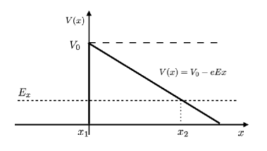
Figure 5: The potential energy inside and outside of a metallic surface when an external electric field $E$ is added.

We now use eqn. $\left(\ref{eq:tunneling}\right)$ to calculate the GUP modified transmission probability. For an electron of energy $E_{x}\leq E_{F}<V_{0}$, there are two turning points:

$$x_{1}=0\text{ and }x_{2}=\frac{V_{0}-E_{x}}{eE}.$$ (43)

The exponent $\eta$ in eqn. $\left(\ref{eq:tunneling}\right)$ is

$$\eta\left(E_{x}\right) \equiv\frac{1}{\hbar}\int_{x_{1}}^{x_{2}}\left|p\left(\sqrt{2m\left[E_{x}-V_{0}+eEx\right]}\right)\right|dx$$

$$\approx\frac{2\sqrt{2m}\left(V_{0}-E_{x}\right)^{\frac{3}{2}}}{3eE\hbar}\left[1-\frac{2m\beta\left(V_{0}-E_{x}\right)}{5}\right],$$ (44)

which gives the transmission probability $T\left(E_{x}\right)\approx e^{-2\eta\left(E_{x}\right)}$.

Next we want to calculate the electric current density in this case. As a consequence of the GUP, the number of quantum states should be changed to APP-Wang:2010ct

$$\frac{Vd^{3}p}{\left(2\pi\hbar\right)^{3}\left(1+\beta p^{2}\right)^{3}},$$ (45)

where $p^{2}=p_{i}p^{i}$. Therefore, the electric current density is given by

$$J=e\int\frac{2dp_{x}dp_{y}dp_{z}}{\left(2\pi\hbar\right)^{3}\left(1+\beta p^{2}\right)^{3}}\frac{p_{x}}{m}T\left(E_{x}\right)$$ (46)

where $E_{x}=\frac{p_{x}^{2}}{2m}$. The range of $p_{x}$, $p_{y}$, are $p_{z}$ are inside the Fermi sphere:

$$p_{x}^{2}+p_{y}^{2}+p_{z}^{2}\leq 2mE_{F}.$$ (47)

To calculate $J$, we use cylindrical coordinates:

$$p_{y}=\rho\cos\phi\text{, }p_{z}=\rho\sin\phi\text{, and }\rho^{2}+p_{x}^{2}\leq 2mE_{F},$$ (48)

and have

$$J =\frac{4\pi e}{\left(2\pi\hbar\right)^{3}}\int_{0}^{\sqrt{2mE_{F}}}\frac{p_{x}}{m}T\left(E_{x}\right)dp_{x}\int_{0}^{\sqrt{2mE_{F}-p_{x}^{2}}}\frac{\rho d\rho}{\left[1+\beta\left(\rho^{2}+p_{x}^{2}\right)\right]^{3}}$$

$$\approx\frac{2\pi e}{\left(2\pi\hbar\right)^{3}}\int_{0}^{\sqrt{2mE_{F}}}\frac{p_{x}}{m}T\left(E_{x}\right)\left(2mE_{F}-p_{x}^{2}\right)\left[1-\frac{3\beta}{2}\left(2mE_{F}+p_{x}^{2}\right)\right]dp_{x}.$$ (49)

To simplify the result, we change $E_{x}$ to

$$\epsilon=E_{F}-E_{x}.$$ (50)

Therefore, one has

$$J\approx\frac{em}{2\pi^{2}\hbar^{3}}\int_{0}^{E_{F}}\epsilon T\left(\epsilon\right)\left[1-3\beta m\left(2E_{F}-\epsilon\right)\right]d\epsilon.$$ (51)

Since $T\left(\epsilon\right)$ decreases rapidly with increasing $\epsilon$, therefore in $T\left(\epsilon\right)$ we can expand $\left(V_{0}-E_{F}+\epsilon\right)^{\frac{3}{2}}$:

$$\left(V_{0}-E_{F}+\epsilon\right)^{\frac{3}{2}}\approx\left(V_{0}-E_{F}\right)^{\frac{3}{2}}+\frac{3}{2}\epsilon\left(V_{0}-E_{F}\right)^{\frac{1}{2}}.$$ (52)

We find

$$J\approx\frac{em}{2\pi^{2}\hbar^{3}}\exp\left[-\frac{2Q}{3}\right]\frac{\left(V_{0}-E_{F}\right)^{2}}{Q^{2}}\left[1+\frac{4\beta m\left(V_{0}-E_{F}\right)Q}{15}\right],$$ (53)

where we extend the range of integration in eqn. $\left(\ref{eq:J}\right)$ to $\left(0,\infty\right)$, and

$$Q=\frac{2\sqrt{2m}\left(V_{0}-E_{F}\right)^{\frac{3}{2}}}{\hbar eE}.$$ (54)

In APP-Depas , the Fowler-Nordheim tunneling in device grade ultra-thin $3$-$6$ nm $n^{+}$poly-Si/SiO₂/$n$-Si structures has been analyzed. Typically for this electron tunnelling, we have

$$Q\sim 10\text{, }V_{0}-E_{F}\sim 1\text{eV, and }m\sim 0.5\text{MeV.}$$ (55)

Therefore from eqn. $\left(\ref{eq:JJ}\right)$, the correction due to GUP is given by

$$\frac{\delta J}{J}\sim 10^{-50}\beta_{0}.$$ (56)

The comparison of the calculated and experimental tunnel current was plotted in FIG. 8 of APP-Depas , which implies $\frac{\delta J}{J}\lesssim 10^{-2}$. Then the upper bound on $\beta_{0}$ follows:

$$\beta_{0}<10^{48}.$$ (57)

IV Conclusions

In this paper, we considered quantum tunneling in the deformed quantum mechanics with a minimal length. We first found one WKB connection formula through a turning point. Then the tunnelling rates through potential barriers were derived using the WKB approximation. Finally, effects of the minimal length on quantum tunneling were discussed in two examples in nuclear and atomic physics, $\alpha$ decay and the Fowler-Nordheim tunnelling. Upper bounds on $\beta_{0}$ were given in these two examples.

- (1) P. K. Townsend, “Small Scale Structure of Space-Time as the Origin of the Gravitational Constant,” Phys. Rev. D 15, 2795 (1977). doi:10.1103/PhysRevD.15.2795
- (2) D. Amati, M. Ciafaloni and G. Veneziano, “Can Space-Time Be Probed Below the String Size?,” Phys. Lett. B 216, 41 (1989). doi:10.1016/0370-2693(89)91366-X
- (3) K. Konishi, G. Paffuti and P. Provero, “Minimum Physical Length and the Generalized Uncertainty Principle in String Theory,” Phys. Lett. B 234, 276 (1990). doi:10.1016/0370-2693(90)91927-4
- (4) L. J. Garay, “Quantum gravity and minimum length,” Int. J. Mod. Phys. A 10, 145 (1995) doi:10.1142/S0217751X95000085 [gr-qc/9403008].
- (5) M. Maggiore, “The Algebraic structure of the generalized uncertainty principle,” Phys. Lett. B 319, 83 (1993) doi:10.1016/0370-2693(93)90785-G [hep-th/9309034].
- (6) A. Kempf, G. Mangano and R. B. Mann, “Hilbert space representation of the minimal length uncertainty relation,” Phys. Rev. D 52, 1108 (1995) doi:10.1103/PhysRevD.52.1108 [hep-th/9412167].
- (7) L. N. Chang, D. Minic, N. Okamura and T. Takeuchi, “The Effect of the minimal length uncertainty relation on the density of states and the cosmological constant problem,” Phys. Rev. D 65, 125028 (2002) doi:10.1103/PhysRevD.65.125028 [hep-th/0201017].
- (8) F. Brau, “Minimal length uncertainty relation and hydrogen atom,” J. Phys. A 32, 7691 (1999) doi:10.1088/0305-4470/32/44/308 [quant-ph/9905033].
- (9) S. Das and E. C. Vagenas, “Universality of Quantum Gravity Corrections,” Phys. Rev. Lett. 101, 221301 (2008) doi:10.1103/PhysRevLett.101.221301 [arXiv:0810.5333 [hep-th]].
- (10) S. Hossenfelder, M. Bleicher, S. Hofmann, J. Ruppert, S. Scherer and H. Stoecker, “Collider signatures in the Planck regime,” Phys. Lett. B 575, 85 (2003) doi:10.1016/j.physletb.2003.09.040 [hep-th/0305262].
- (11) A. F. Ali, S. Das and E. C. Vagenas, “Discreteness of Space from the Generalized Uncertainty Principle,” Phys. Lett. B 678, 497 (2009) doi:10.1016/j.physletb.2009.06.061 [arXiv:0906.5396 [hep-th]].
- (12) X. Li, “Black hole entropy without brick walls,” Phys. Lett. B 540, 9 (2002) doi:10.1016/S0370-2693(02)02123-8 [gr-qc/0204029].
- (13) F. Brau and F. Buisseret, “Minimal Length Uncertainty Relation and gravitational quantum well,” Phys. Rev. D 74, 036002 (2006) doi:10.1103/PhysRevD.74.036002 [hep-th/0605183].
- (14) P. Wang, H. Yang and S. Ying, “Minimal length effects on entanglement entropy of spherically symmetric black holes in the brick wall model,” Class. Quant. Grav. 33, no. 2, 025007 (2016) doi:10.1088/0264-9381/33/2/025007 [arXiv:1502.00204 [gr-qc]].
- (15) S. Hossenfelder, “Minimal Length Scale Scenarios for Quantum Gravity,” Living Rev. Rel. 16, 2 (2013) doi:10.12942/lrr-2013-2 [arXiv:1203.6191 [gr-qc]].
- (16) T. V. Fityo, I. O. Vakarchuk and V. M. Tkachuk, “WKB approximation in deformed space with minimal length,” J. Phys. A 39, no. 2, 379 (2006). doi:10.1088/0305-4470/39/2/0088
- (17) J. Z. Simon, “Higher Derivative Lagrangians, Nonlocality, Problems and Solutions,” Phys. Rev. D 41, 3720 (1990). doi:10.1103/PhysRevD.41.3720
- (18) B. Mu, P. Wang and H. Yang, “Thermodynamics and Luminosities of Rainbow Black Holes,” JCAP 1511, no. 11, 045 (2015) doi:10.1088/1475-7516/2015/11/045 [arXiv:1507.03768 [gr-qc]].
- (19) J. Tao, P. Wang and H. Yang, “Homogeneous Field and WKB Approximation In Deformed Quantum Mechanics with Minimal Length,” Adv. High Energy Phys. 2015, 718359 (2015) doi:10.1155/2015/718359 [arXiv:1211.5650 [hep-th]].
- (20) G. Gamow, “Zur Quantentheorie des Atomkernes,” Z. Phys. 51, 204 (1928). doi:10.1007/BF01343196
- (21) H. Geiger, J. M. Nuttall, “The ranges of the particles from various radioactive substances and a relation between range and period of transformation,” Philos. Mag. 22, 613 (1911).
- (22) G. Blado, T. Prescott, J. Jennings, J. Ceyanes and R. Sepulveda, “Effects of the Generalized Uncertainty Principle on Quantum Tunneling,” Eur. J. Phys. 37, 025401 (2016) doi:10.1088/0143-0807/37/2/025401 [arXiv:1509.07359 [quant-ph]].
- (23) R. H. Fowler and L. Nordheim, “Electron emission in intense electric fields,” Proc. Roy. Soc. Lond. A 119, 173 (1928). doi:10.1098/rspa.1928.0091
- (24) P. Wang, H. Yang and X. Zhang, “Quantum gravity effects on statistics and compact star configurations,” JHEP 1008 (2010) 043 doi:10.1007/JHEP08(2010)043 [arXiv:1006.5362 [hep-th]].
- (25) M. Depas, B. Vermeire, P. W. Mertens, R. L. Van Meirhaeghe and M. M. Heyns, “Determination of tunneling parameters in ultra-thin oxide layer poly-Si/SiO2/Si structures,” Solid-State Electronics, vol. 38, pp. 1465-1471, Aug. 1995.