Phase diagram of the off-diagonal Aubry-André model
Abstract
We study a one-dimensional quasiperiodic system described by the off-diagonal Aubry-André model and investigate its phase diagram by using the symmetry and the multifractal analysis. It was shown in a recent work (Phys. Rev. B 93, 205441 (2016)) that its phase diagram was divided into three regions, dubbed the extended, the topologically-nontrivial localized and the topologically-trivial localized phases, respectively. Out of our expectation, we find an additional region of the extended phase which can be mapped into the original one by a symmetry transformation. More unexpectedly, in both “localized” phases, most of the eigenfunctions are neither localized nor extended. Instead, they display critical features, that is, the minimum of the singularity spectrum is in a range instead of for the localized state or for the extended state. Thus, a mixed phase is found with a mixture of localized and critical eigenfunctions.
pacs:
71.23.An, 71.23.Ft, 05.70.JkI Introduction
Since Anderson’s seminal paper in 1958 1an the metal-insulator transition has been studied in a wide range of systems. The scaling theory 2scal predicts that there is no metal-insulator transition in one-dimensional (1D) systems with randomly-distributed impurities. On the other hand, 1D quasiperiodic systems 1PRB ; 2PRA ; 3PRA ; He ; Gramsch can host localized, extended or critical eigenstates. The Aubry-André (AA) model 7aubry is an important paradigm of 1D quasiperiodic systems. It can be derived from the reduction of a two-dimensional quantum Hall system in the magnetic field 20SU . Due to recent advances in experimental techniques, the AA model has been realized in ultracold atoms 8BILLY ; 9ROATI and photonic crystals 10PRL ; 11PRL . The phase diagram of the AA model has been well understood with extensive researches 21SO ; 22SOU ; 23ZD ; 24GE ; 25MA ; 26WI . And many different variations of the AA model were studied also. By including a long-range hopping term or modulating the on-site potentials, some authors found a mobility edge in the spectrum which can be precisely addressed by the duality symmetry 12PRL ; 13PRL . The others addressed a transition from the topological superconducting phase to the localized phase in the AA model with p-wave pairing interaction 14PRL ; 15PRL ; 16PRB ; Cao .
Among different variations, the off-diagonal Aubry-André model displays an abundant phase diagram. It brings up either the zero-energy topological edge modes 17PRL or preserves the critical states in a large parameter space 18PRB , depending on different ways of modulating the nearest-neighbor hopping amplitude.
In a very recent paper 19PRB , the authors combined both the commensurate and incommensurate modulations to explore the corresponding phase diagram. The model Hamiltonian is expressed as
| (1) |
where is a fermionic annihilation operator, is the total number of sites, and and denote the commensurate and incommensurate modulations, respectively. A typical choice of the parameters is , and . For convenience, is set as the energy unit.
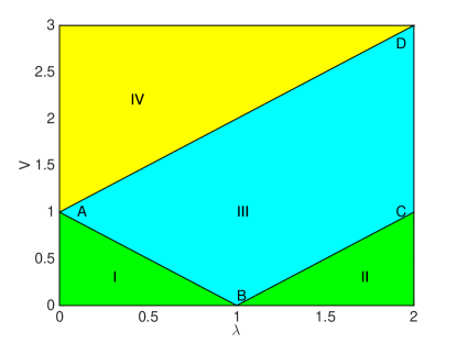
It was argued that the phase diagram of this model can be divided into three regions, which are the extended, the topologically-nontrivial localized and the topologically-trivial localized phases, respectively. In this paper we revisit this model by using the symmetry and the multifractal analysis. Our findings are summarized in the phase diagram (Fig. 1). The main results includes (i) there exists an additional region of extended phase (region II) which can be mapped into region I by a newly-discovered symmetry transformation, and (ii) region III and IV are mixed phases instead of localized phases in which most of the eigenstates are critical states.
The rest of the paper is organized as follows. In Sec. II, we present the symmetry transformation for Hamiltonian (1), and use it to determine the boundaries between different phases. We further show that region I and II are in the extended phase by calculating the inverse participation ratio numerically. In Sec. III, we apply the multifractal analysis in two different approaches. In both approaches we verify that region III and IV are mixed phases with most of the eigenstates being critical states.
II Symmetry transformation and inverse participation ratio
We identify the phase boundaries of the off-diagonal Aubry-André model by finding its symmetry transformation. For our purpose, the Schrödinger equation is expressed every four sites as
| (2) |
where denotes the eigenfunction in the first-quantization language and is the eigenenergy. is an arbitrary integer. We find a transformation with a period of four sites which keeps the Schrödinger equation invariant. The transformation is , , , , , and . This transformation changes the sign of the wave function, but has no influence on whether the wave function is localized or not. The shift of by keeps the absolute value of invariant at each site. Therefore, as we exchange and while keeping invariant the wave function only changes the sign at some sites. The transformation of from to does not change whether the eigenstate is localized or extended. Furthermore, multiplying the Hamiltonian by an arbitrary number does not change its eigenfunctions. As is fixed, the simultaneous transformation and must relate two points in the phase diagram that belong to the same phase.
Under this transformation, region I in the phase diagram (Fig. 1) is mapped into region II. For example, the boundary (), after the transformation, becomes (). Especially, all the region below the boundary can be mapped into the region below . Therefore, region I and II are dual and belong to the same phase. The boundary is . It keeps invariant under the symmetry transformation. Region III and IV are both mapped into themselves under the symmetry transformation.
By numerically calculating the inverse participation ratio (IPR) and the mean inverse participation ratio (MIPR), we find that region I and II are both the extended phase. The IPR of a normalized wave function is defined as 27TH ; 28KO
| (3) |
where denotes the total number of sites and is the energy level index. It is well known that the IPR of an extended state scales like which goes to in thermodynamic limit. But for a localized state IPR is finite even in thermodynamic limit. For a critical state IPR scales as with . There are different eigenfunctions for a specific Hamiltonian. We then define the mean inverse participation ratio (MIPR) as
| (4) |
where denotes the IPR of the th eigenstate.
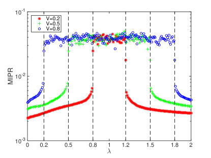
In Fig. 2, we plot MIPR as a function of at three disorder amplitudes: , , and . Here we used . There are two turning points of MIPR located at and , respectively. At the turning points MIPR becomes very steep. We also checked that with increasing number of sites the change of MIPR at the turning points becomes even sharper. In the thermodynamic limit , a singularity behavior of MIPR is expected signaling a transition between the extended phase and the localized (or critical) phase. So the thermodynamically vanishing MIPR suggests that the system is in the extended regions for and .
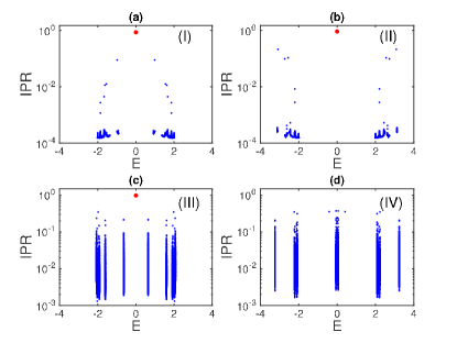
We further study the distribution of IPR with different eigenstates. The results are plotted in Fig. 3. We find the zero-energy modes (the red dots) in the region I, II and III. Thus, these three regions are in the topologically-nontrivial phase. But region IV is topologically trivial. Fig. 3(a) and Fig. 3(b) plot the IPR distribution in region I and II, respectively. The distribution has the same characteristics in these two regions. For almost all the eigenstates, their IPR are close to each other, being very low (around ). This indicates that region I and II has a pure energy spectrum, that all the eigenstates are extended. The extended, critical and localized states do not coexist in these two regions.
On the other hand, region III and IV have the significantly different IPR distribution (see Fig. 3(c) and Fig. 3(d)). In these two regions, the value of IPR is at least one order of magnitude larger than that of the extended state (). At the same time, the IPRs of different eigenstates disperse widely in a range over two orders of magnitude (from to ). Such a dispersed distribution suggests that region III and IV should not be the pure localized phase. Instead, there should exist critical states in these two regions. To clarify the nature of them, we will apply the multifractal analysis to the eigenfunctions in next section.
III Multifractal analysis
We carry out the multifractal analysis in two different approaches. In the first approach, we fix the total number of sites in the system, while dividing the system into a series of boxes with the box length tunable. This is called the box-counting method 29SI ; 30HU . In the second approach, we obtain the scaling behavior of the wave functions by changing the total number of sites.
III.1 Box-counting method
Let us consider a normalized wave function defined over a chain of sites. The probability of finding the particle at site is given by which satisfies . In the multifractal analysis of wave functions, is viewed as an increase at site for the eigenvalue. And the increase is supposed to satisfy a local power law everywhere along the chain.
We divide the chain into segments with each segment containing sites. The total increase in the th segment is given by . We then introduce a partition function
| (5) |
The partition function obeys a power law where the exponent is related to the multifractal dimension by . Following previous literatures we set . It has been found that tends to for a localized state but to for an extended state. signals a critical state.
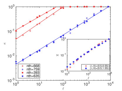
We select two typical points in region III and IV, which are and , respectively. Fig. 4 plots the corresponding as a function of on the logarithmic scale. By carefully checking the eigenstates in region III and IV, we find that the system has a mixed spectrum either of a localized or of a critical eigenstate. Here we take few typical eigenstates as examples. For the th eigenstate at (red crosses in Fig. 4), scales as as , but tends to 0 for larger segment. The existence of a turning point in the curve of is the typical feature of a localized state. Indeed, the localized states display multifractal feature up to the localization length. Similarly, the th eigenstate at is also a localized state (see red stars in Fig. 4). But for the th eigenstate at (blue crosses) and the th eigenstate at (blue stars), scales as over the whole domain of . The lack of turning point and a fractional together indicate that these two states are critical. Therefore, in region III and IV the system has a mixed spectrum in which the localized and critical states coexist.
We further study the average of over different eigenstates, defined as
| (6) |
where denotes the partition function of the th eigenstate. The inset of Fig. 4 plots as a function of on the logarithmic scale. In both region III and IV, scales approximately as over the whole domain of . No obvious turning point is found. And is a fraction. This indicates that most of the eigenstates in region III and IV are critical states. Otherwise, would have a turning point and display a platform for larger . Because for larger , tends to 0 for a localized state but bigger than 0 for a critical state. If there were a significant fraction of localized states in the spectrum, their contribution to would dominate, and would then display a platform.
It is worth mentioning that the Legendre transformation of is no more than the singularity spectrum. The latter is an important quantity characterizing the multifractal nature of the system. We will discuss the singularity spectrum in next subsection. Considering numerical stability, we will employ a different method for calculating it.
III.2 Finite size scaling
In the box-counting method, the segment length is tunable. An extreme case is that each segment contains only a single site. The segment length is then . Note that the length of the whole chain is usually normalized to unity in the multifractal analysis. Therefore, the segment length can also be changed by changing the total number of sites . According to previous works 1PRB ; 31HI ; 32WA , it is convenient to choose where is the th Fibonacci number. The advantage of this choice is that the golden ratio can be expressed as .
In a multifractal system the increase at any site satisfies a local power law:
| (7) |
where is the singularity exponent. The set of sites that share the same singularity exponent is a fractal set of dimension . is just the so-called singularity spectrum. The approach of obtaining is summarized as follows. The partition function is now defined as . We then introduce the free energy . The singularity spectrum is the Legendre transformation of the free energy, given by
| (8) |
with and . For a critical wave function, is nonzero in an interval in which changes continuously. In the thermodynamic limit , the value of can be used to distinguish the extended state (), the localized state () and the critical state (). Since there are eigenstates for each Hamiltonian, we use the average of over all the eigenstates as the indicator, which is denoted by .
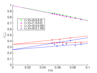
We plot as a function of for different in Fig. 5. We find that extrapolates to for and which are both in the extended phase. This fits our expectation. extrapolates to for , and to for . The fractional is another evidence that most of the states in region III and IV are critical states.
IV Conclusions
In summary, we clarify the phase diagram of the off-diagonal AA model. For this purpose, we discovered a symmetry transformation which changes the sign of the wave function but keeps its amplitude invariant. We also apply the box-counting and the finite size scaling methods in analyzing the eigenfunctions. These two different approaches both show that the wave functions display multifractal behavior. We believe that the methods employed in this paper are useful in a wide range of variations of the AA model.
Acknowledgements.
This work was supported by the NSF of Zhejiang Province (Grant No. Z15A050001), the NSF of China (Grant Nos. 11374266 and 11304280), and the Program for New Century Excellent Talents in University.References
- (1) P. W. Anderson, Phys. Rev. 109, 1492 (1958).
- (2) E. Abrahams, P. W. Anderson, D. C. Licciardello, and T. V. Ramakrishnan, Phys. Rev. Lett. 42, 673 (1979).
- (3) M. Kohmoto and D. Tobe, Phys. Rev. B 77, 134204 (2008).
- (4) X. Cai, S. Chen, and Y. Wang, Phys. Rev. A 81, 023626 (2010).
- (5) L. Zhou, H. Pu, and W. Zhang, Phys. Rev. A 87, 023625 (2013).
- (6) K. He, I. I. Satija, C. W. Clark, A. M. Rey, and M. Rigol, Phys. Rev. A 85, 013617 (2012).
- (7) C. Gramsch and M. Rigol, Phys. Rev. A 86, 053615 (2012).
- (8) S. Aubry and G. André, Ann. Israel Phys. Soc. 3, 133 (1980).
- (9) I. M. Suslov, Zh. Eksp. Teor. Fiz. 83, 1079 (1982).
- (10) J. Billy, V. Josse, Z. Zuo, A. Bernard, B. Hambrecht, P. Lugan, D. Clément, L. Sanchez-Palencia, P. Bouyer, and A. Aspect, Nature 453, 891 (2008).
- (11) G. Roati, C. D’Errico, L. Fallani, M. Fattori, C. Fort, M. Zaccanti, G. Modugno, M. Modugno, and M. Inguscio, Nature 453, 895 (2008).
- (12) Y. Lahini, R. Pugatch, F. Pozzi, M. Sorel, R. Morandotti, N. Davidson, and Y. Silberberg, Phys. Rev. Lett. 103, 013901 (2009).
- (13) Y. E. Kraus, Y. Lahini, Z. Ringel, M. Verbin, and O. Zilberberg, Phys. Rev. Lett. 109, 106402 (2012).
- (14) J. B. Sokoloff, Phys. Rep. 126, 189 (1985).
- (15) C. M. Soukoulis and E. N. Economou, Phys. Rev. Lett. 48, 1043 (1982).
- (16) A. D. Zdetsis, C. M. Soukoulis, and E. N. Economou, Phys. Rev. B 33, 4936 (1985).
- (17) T. Geisel, R. Ketzmerick, and G. Petschel, Phys. Rev. Lett. 66,1651 (1991).
- (18) K. Machida and M. Fujita, Phys. Rev. B 34, 7367 (1986).
- (19) M. Wilkinson, Proc. R. Soc. Lond. A 391, 305 (1984).
- (20) S. Ganeshan, J. H. Pixley, and S. Das Sarma, Phys. Rev. Lett. 114, 146601 (2015).
- (21) J. Biddle and S. Das Sarma, Phys. Rev. Lett. 104, 070601 (2010).
- (22) X. Cai, L.-J. Lang, S. Chen, and Y. Wang, Phys. Rev. Lett. 110, 176403 (2013).
- (23) W. DeGottardi, D. Sen, and S. Vishveshwara, Phys. Rev. Lett. 110, 146404 (2013).
- (24) J. Wang, X.-J. Liu, G. Xianlong, and H. Hu, Phys. Rev. B 93, 104504 (2016).
- (25) Y. Cao, G. Xianlong, X.-J. Liu, and H. Hu, Phys. Rev. A 93, 043621 (2016).
- (26) S. Ganeshan, K. Sun, and S. Das Sarma, Phys. Rev. Lett. 110, 180403 (2013).
- (27) F. Liu, S. Ghosh, and Y. D. Chong, Phys. Rev. B 91, 014108 (2015).
- (28) J. C. C. Cestari, A. Foerster, and M. A. Gusmão, Phys. Rev. B 93, 205441 (2016).
- (29) D. J. Thouless, J. Phys. C 5, 77 (1972).
- (30) M. Kohmoto, Phys. Rev. Lett 51, 1198 (1983).
- (31) A. P. Siebesma and L. Pietronero, Europhys.Lett. 4, 597 (1987).
- (32) B. Huckestein and L. Schweitzer, Phys. Rev. Lett. 72, 713 (1994).
- (33) H. Hiramoto, M. Kohmoto, Phys. Rev. B 40, 8225 (1989).
- (34) Y. Wang, Y. Wang, and S. Chen, arxiv:1603.09206 (2016).