Quantum Neural Machine Learning - Backpropagation and Dynamics

Abstract

The current work addresses quantum machine learning in the context of Quantum Artificial Neural Networks such that the networks’ processing is divided in two stages: the learning stage, where the network converges to a specific quantum circuit, and the backpropagation stage where the network effectively works as a self-programing quantum computing system that selects the quantum circuits to solve computing problems. The results are extended to general architectures including recurrent networks that interact with an environment, coupling with it in the neural links’ activation order, and self-organizing in a dynamical regime that intermixes patterns of dynamical stochasticity and persistent quasiperiodic dynamics, making emerge a form of noise resilient dynamical record.

Keywords: Quantum Artificial Neural Networks, Machine Learning, Open Quantum Systems, Complex Quantum Systems

University of Lisbon, Institute of Social and Political Sciences, cgoncalves@iscsp.ulisboa.pt

1 Introduction

Quantum Artificial Neural Networks (QuANNs) provide an approach to quantum machine learning based on networked quantum computation (Chrisley, 1995; Kak, 1995; Menneer and Narayanan, 1995; Behrman et al., 1996; Menneer, 1998; Ivancevic and Ivancevic, 2010; Schuld et al., 2014a; Schuld et al., 2014b; Gonçalves, 2015a, 2015b).

In the current work, we address two major building blocks for quantum neural machine learning: feedforward dynamics and quantum backpropagation, introduced as a quantum circuit selection control dynamics that introduces a feeding back of the neural network, thus, after propagating quantum information in the feedforward direction, during the quantum learning stage, quantum information is, then, propagated backwards so that the network effectively functions as a self-programming quantum computing system, efficiently solving computational problems.

The concept of quantum neural backpropagation with which we work is different from the classical ANNs’ error backpropagation. The quantum backpropagation dynamics is integrated in a two stage neural cognition scheme: there is a feedforward learning stage such that the output neurons’ states, initially separable from the input neurons’ states, converge during a neural processing time $\triangle t_{o}$ to correlated states with the input layer, and then there is a backpropagation stage, where the output neurons act as a control system that triggers different quantum circuits that are implemented on the input neurons, conditionally transforming their state in such a way that a given computational problem is solved.

The approach to quantum machine learning that we assume here is, therefore, worked from a notion of measurement-based quantum machine learning, where the learning stage corresponds to a quantum measurement dynamics, in which the system records the state of the target, in order to later use that record for solving some task that involves the conditional transformation of the target’s state, conditional, in this case, on the computational record.

In the present work, we first show (section 2) how this approach to quantum machine learning can be integrated, within a supervised learning setting, in feedforward neural networks, to solve computational problems. We, thus, begin by introducing an Hamiltonian framework for quantum neural machine learning with basic feedforward neural networks (subsection 2.1), integrating quantum measurement theory and dividing the quantum neural dynamics in the learning stage and the backpropagation stage, we then apply the framework to two example problems: the firing pattern selection problem (addressed in subsection 2.2.), where the neural network places the input layer in a specific well-defined firing configuration, from an initially arbitrary superposition of neural firing patterns, the n-to-m Boolean functions’ representation problem (addressed in subsection 2.3), where the goal for the network is to correct the input layer so that it represents an arbitrary n-to-m Boolean function. The first problem is solved with a network size equal to $2m$ (where $m$ is the size of the input layer), the second problem is solved for a network size of $n+2m$.

In section 3, the results from section 2 are expanded to more general architectures that can be represented by any finite digraph (subsection 3.1) dealing with an unsupervised learning framework, where the network’s neural processing is comprised of feedforward computations and backpropagation dynamics that close recurrent loops. We address how these networks compute an environment in terms of the iterated activation of the network, such that the computation is conditional on the neural links’ activation order.

Section 3’s computational framework is, therefore, that of open systems quantum computation with changing orders of gates. The changing orders of gates comes from Aharonov et al.’s (1990) original work on superpositions of time evolutions of quantum systems, and has received recent attention regarding the possibility of quantum computation with greater computing power than the fixed quantum circuit model (Procopio, et al., 2015; Brukner, 2014; Chiribella, et al., 2013). The main advantage of this approach is that it allows the research on how a QuANN may process an environment without giving it a specific final state goal that may direct its computation, thus, the QuANN behaves as an (artificial) complex adaptive system that responds to the environment solely based on its networked architecture and the initial state of the environment plus network. In this case, the way in which the network responds to the environment must be analyzed at the level of the different emergent dynamics for the network’s quantum averages.

In subsection 3.2, we analyze the mean total neural firing energy’s emergent dynamics, for an example of a recurrent neural network, showing that the computation of the environment by the network makes emerge complex neural dynamics that combine elements of regularity, in the form of persistent quasiperiodic recurrences, and elements of emergent dynamical stochasticity (a form of emergent neural noise), the presence of both elements at the level of the mean total neural firing energy shares dynamical signatures akin to the edge of chaos dynamics found in classical cellular automata and nonlinear dynamical systems (Packard, 1988; Crutchfield and Young, 1990; Langton, 1990; Wolfram, 2002), random Boolean networks (Kauffman and Johnsen, 1991; Kauffman, 1993) and classical neural networks (Gorodkin et al., 1993; Bertschinger and Natschläger, 2004).

The quasiperiodic recurrences constitute a form of “noise” resilient dynamical record. We also find, in the simulations, patterns that are closer to a noisy chaotic regime, as well as stronger resilient quasiperiodic patterns with toroidal attractors that show up in the mean energy dynamics.

In section 4, a final reflection is provided on the article’s main results including the relation of section 3’s results and research on classical neural networks.

2 Quantum Neural Machine Learning

2.1 Learning and Backpropagation in Feedforward Networks

In classical ANNs, a neuron with a binary firing activity can be described in terms a binary alphabet $\mathbb{A}_{2}=\left\{0,1\right\}$, with $0$ representing a nonfiring neural state and $1$ representing a firing neural state. For QuANNs, on the other hand, the neuron’s quantum neural states are described by a two-dimensional Hilbert Space $\mathcal{H}_{2}$, spanned by the computational basis $\mathcal{B}_{2}=\left\{\left|0\right\rangle,\left|1\right\rangle\right\}$, where $\left|0\right\rangle$ encodes a nonfiring neural state and $\left|1\right\rangle$ encodes a firing neural state. These states have a physical description as the eigenstates of a neural firing Hamiltonian:

$$\hat{H}=\frac{2\pi}{\tau}\hbar\left(\frac{\hat{1}-\hat{\sigma}_{3}}{2}\right)$$ (1)

where $\tau$ is measured seconds, so that the corresponding neural firing frequency given by $(1/\tau)$Hz, and $\hat{\sigma}_{3}$ is Pauli’s operator:

$$\hat{\sigma}_{3}=\left|0\right\rangle\left\langle 0\right|-\left|1\right\rangle\left\langle 1\right|=\left(\begin{array}[]{cc}1&0\\ 0&-1\end{array}\right)$$ (2)

The computational basis $\mathcal{B}_{2}$, then, satisfies the eigenvalue equation:

$$\hat{H}\left|r\right\rangle=\frac{2\pi}{\tau}\hbar r\left|r\right\rangle$$ (3)

with $r=0,1$. Thus, the nonfiring state corresponds to an energy eigenstate of zero Joules and the firing state corresponds to an energy eigenstate of $\hbar 2\pi/\tau$ Joules. In the special case where the neural firing frequency is such that the following condition holds:

$$\frac{2\pi}{\tau}\hbar=1\textrm{J}$$ (4)

then, the nonfiring energy eigenvalue is zero Joules (0J) and the firing eigenvalue is one Joule (1J). In this special case, the numbers associated to the ket vector notation $\left|0\right\rangle$ and $\left|1\right\rangle$, which usually take the role of logical values (bits) in standard quantum computation, coincide exactly with the energy eigenvalues of the quantum artificial neuron. The three Pauli operators’ actions on the neuron’s firing energy eigenstates are given, respectively, by:

$$\hat{\sigma}_{1}\left|r\right\rangle=\left|1-r\right\rangle$$ (5)

$$\hat{\sigma}_{2}\left|r\right\rangle=i(-1)^{r}\left|1-r\right\rangle$$ (6)

$$\hat{\sigma}_{3}\left|r\right\rangle=(-1)^{r}\left|r\right\rangle$$ (7)

with $\hat{\sigma}_{3}$ described by Eq.(2) and $\hat{\sigma}_{1}$, $\hat{\sigma}_{2}$ defined as:

$$\hat{\sigma}_{1}=\left|0\right\rangle\left\langle 1\right|+\left|1\right\rangle\left\langle 0\right|=\left(\begin{array}[]{cc}0&1\\ 1&0\end{array}\right)$$ (8)

$$\hat{\sigma}_{2}=-i\left|0\right\rangle\left\langle 1\right|+i\left|1\right\rangle\left\langle 0\right|=\left(\begin{array}[]{cc}0&-i\\ i&0\end{array}\right)$$ (9)

A neural network with $N$ neurons has, thus, an associated Hilbert space, given by the $N$-tensor product of copies of $\mathcal{H}_{2}$: $\mathcal{H}_{2}^{\otimes N}$, which is spanned by the basis $\mathcal{B}_{2}^{\otimes N}=\left\{\left|\mathbf{r}\right\rangle:\mathbf{r}\in\mathbb{A}_{2}^{N}\right\}$, where $\mathbb{A}_{2}^{N}$ is the set of all length $N$ binary strings: $\mathbb{A}_{2}^{N}=\left\{r_{1}r_{2}...r_{N}:r_{k}\in\mathbb{A}_{2},k=1,2,...,N\right\}$. The basis $\mathcal{B}_{2}^{\otimes N}$ corresponds to the set of well-defined firing patterns for the neural network, which coincide with the classical states of a corresponding classical ANN, the general state of the quantum network can, however, exhibit a superposition of neural firing patterns described by a normalized ket vector, in the space $\mathcal{H}_{2}^{\otimes N}$, defined as:

$$\left|\psi\right\rangle=\sum_{\mathbf{r}\in\mathbb{A}_{2}^{N}}\psi(\mathbf{r})\left|\mathbf{r}\right\rangle$$ (10)

with the normalization condition:

$$\sum_{\mathbf{r}\in\mathbb{A}_{2}^{N}}|\psi(\mathbf{r})|^{2}=1$$ (11)

For such an $N$ neuron network we can introduce the local operators for $k=1,2,...,N$:

$$\hat{H}_{k}=\hat{1}^{\otimes(k-1)}\otimes\hat{H}\otimes\hat{1}^{\otimes(N-k)}$$ (12)

with $\hat{H}_{1}=\hat{H}\otimes\hat{1}^{\otimes(N-1)}$ and $\hat{H}_{N}=\hat{1}^{\otimes(N-1)}\otimes\hat{H}$, where $\hat{H}$ has the structure defined in Eq.(1) and $\hat{1}=\left|0\right\rangle\left\langle 0\right|+\left|1\right\rangle\left\langle 1\right|$ is the unit operator on $\mathcal{H}_{2}$. The network’s total Hamiltonian $\hat{H}_{Net}$ is, thus, given by the sum:

$$\hat{H}_{Net}=\sum_{k=1}^{N}\hat{H}_{k}$$ (13)

which yields the Hamiltonian for the total neural firing energy, satisfying the equation:

$$\hat{H}_{Net}\left|r_{1}r_{2}...r_{N}\right\rangle=\left(\sum_{k=1}^{N}\frac{2\pi}{\tau}\hbar r_{k}\right)\left|r_{1}r_{2}...r_{N}\right\rangle$$ (14)

An elementary example of a QuANN is the two-layer feedforward network composed of a system of $m$ input neurons and $n$ output neurons. The output neurons are transformed conditionally on the input neurons’ states, so that the neural network has an associated neural links’ operator with the structure:

$$\hat{L}_{\triangle t}=\sum_{\mathbf{r}\in\mathbb{A}_{2}^{m}}\left|\mathbf{r}\right\rangle\left\langle\mathbf{r}\right|\bigotimes_{k=1}^{n}e^{-\frac{i}{\hbar}\triangle t\hat{H}_{k,\mathbf{r}}}$$ (15)

where $\triangle t$ is a neural processing period and the conditional Hamiltonians $\hat{H}_{k,\mathbf{r}}$ are operators on $\mathcal{H}_{2}$ with the general structure given by:

$$\hat{H}_{k,\mathbf{r}}=-\frac{\hbar}{2}\frac{\omega_{k}(\mathbf{r})}{\triangle t_{o}}\hat{1}+\frac{\theta_{k}(\mathbf{r})}{\triangle t_{o}}\sum_{j=1}^{3}u_{j,k}(\mathbf{r})\frac{\hbar}{2}\hat{\sigma}_{j}$$ (16)

such that the angles $\omega_{k}(\mathbf{r})$ and $\theta_{k}(\mathbf{r})$ are measured in radians and $\triangle t_{o}$ is a learning period measured in seconds (the time interval $\triangle t_{o}$ will play here a role analogous to the inverse of the learning rate of classical ANNs), the $u_{j,k}(\mathbf{r})$ terms are the components of a real unit vector $\mathbf{\hat{u}}_{k}(\mathbf{r})$ and $\hat{\sigma}_{j}$ are Pauli’s operators. Thus, the conditional unitary evolution for each output neuron’s state, expressed by the neural links’ operator, is given by the conditional U(2) transformations:

$$e^{-\frac{i}{\hbar}\triangle t\hat{H}_{k,\mathbf{r}}}=e^{i\frac{\omega_{k}(\mathbf{r})\triangle t}{2\triangle t_{o}}}\hat{U}_{\hat{\mathbf{u}}_{k}(\mathbf{r})}\left[\frac{\theta_{k}(\mathbf{r})\triangle t}{\triangle t_{o}}\right]$$ (17)

with the rotation operators defined as:

$$\hat{U}_{\hat{\mathbf{u}}_{k}(\mathbf{r})}\left[\frac{\theta_{k}(\mathbf{r})\triangle t}{\triangle t_{o}}\right]=$$ (18)

$$=\cos\left(\frac{\theta_{k}(\mathbf{r})\triangle t}{2\triangle t_{o}}\right)\hat{1}-i\sin\left(\frac{\theta_{k}(\mathbf{r})\triangle t}{2\triangle t_{o}}\right)\sum_{j=1}^{3}u_{j,k}(\mathbf{r})\hat{\sigma}_{j}$$

where the phase transform angles $\omega_{k}(\mathbf{r})$, the rotation angles $\theta_{k}(\mathbf{r})$ and the unit vectors $\hat{\mathbf{u}}_{k}(\mathbf{r})$ can be different for different output neurons, so that each output neuron’s state is transformed conditionally on the input layer’s neurons’ firing patterns. Depending on the Hamiltonian parameters, we can have a full connection, where the parameters’ values are different for each different input layer’s firing pattern, or local connections, where the Hamiltonian parameters only depend on some of the input neurons’ firing patterns.

The operator $\hat{L}_{\triangle t}$ is, thus, given by:

$$\hat{L}_{\triangle t}=\sum_{\mathbf{r}\in\mathbb{A}_{2}^{m}}\left|\mathbf{r}\right\rangle\left\langle\mathbf{r}\right|\bigotimes_{k=1}^{n}e^{-\frac{i}{\hbar}\triangle t\hat{H}_{k,\mathbf{r}}}=$$ (19)

$$=\sum_{\mathbf{r}\in\mathbb{A}_{2}^{m}}\left|\mathbf{r}\right\rangle\left\langle\mathbf{r}\right|\bigotimes_{k=1}^{n}e^{i\frac{\omega_{k}(\mathbf{r})\triangle t}{2\triangle t_{o}}}\hat{U}_{\hat{\mathbf{u}}_{k}(\mathbf{r})}\left[\frac{\theta_{k}(\mathbf{r})\triangle t}{\triangle t_{o}}\right]$$

For $\triangle t\rightarrow\triangle t_{o}$, the unitary evolution operators described by Eqs.(17) and (18) converge to the result:

$$e^{-\frac{i}{\hbar}\triangle t_{o}\hat{H}_{k,\mathbf{r}}}=$$ (20)

$$=e^{i\frac{\omega_{k}(\mathbf{r})}{2}}\hat{U}_{\hat{\mathbf{u}}_{k}(\mathbf{r})}\left[\theta_{k}(\mathbf{r})\right]=$$

$$=e^{i\frac{\omega_{k}(\mathbf{r})}{2}}\left[\cos\left(\frac{\theta_{k}(\mathbf{r})}{2}\right)\hat{1}-i\sin\left(\frac{\theta_{k}(\mathbf{r})}{2}\right)\sum_{j=1}^{3}u_{j,k}(\mathbf{r})\hat{\sigma}_{j}\right]$$

Assuming, now, an initial state for the neural network given by the general structure:

$$\left|\psi_{0}\right\rangle=\sum_{\mathbf{r}\in\mathbb{A}_{2}^{m}}\psi_{0}(\mathbf{r})\left|\mathbf{r}\right\rangle\bigotimes_{k=1}^{n}\left|\phi_{k}\right\rangle$$ (21)

with $\left|\phi_{k}\right\rangle=\phi_{k}(0)\left|0\right\rangle+\phi_{k}(1)\left|1\right\rangle$, then, the state after a neural processing period of $\triangle t$ is given by:

$$\left|\psi_{\triangle t}\right\rangle=\hat{L}_{\triangle t}\left|\psi_{0}\right\rangle=$$ (22)

$$=\sum_{\mathbf{r}\in\mathbb{A}_{2}^{m}}\psi_{0}(\mathbf{r})\left|\mathbf{r}\right\rangle\bigotimes_{k=1}^{n}e^{-\frac{i}{\hbar}\triangle t\hat{H}_{k,\mathbf{r}}}\left|\phi_{k}\right\rangle$$

From, Eq.(20), as $\triangle t\rightarrow\triangle t_{o}$ the neural network’s state converges to:

$$\left|\psi_{\triangle t_{o}}\right\rangle=$$ (23)

$$=\sum_{\mathbf{r}\in\mathbb{A}_{2}^{m}}\psi_{0}(\mathbf{r})\left|\mathbf{r}\right\rangle\bigotimes_{k=1}^{n}e^{i\frac{\omega_{k}(\mathbf{r})}{2}}\hat{U}_{\hat{\mathbf{u}}_{k}(\mathbf{r})}\left[\theta_{k}(\mathbf{r})\right]\left|\phi_{k}\right\rangle$$

so that each ouput neuron’s state undergoes a parametrized U(2) transformation that is conditional on the input neurons’ firing patterns.

A specific framework for the neural state transition, during the learning period, can be implemented, assuming the state for each output neuron at the beginning of the learning period to be given by:

$$\left|\phi_{k}\right\rangle=\left|+\right\rangle=\frac{\left|0\right\rangle+\left|1\right\rangle}{\sqrt{2}}$$ (24)

In the context of supervised learning, a computational problem with expression in terms of binary firing patterns can be addressed, as illustrated in the next subsections, by introducing functions of the form $f_{k}:\mathbf{\mathbb{A}}_{2}^{m}\rightarrow\mathbb{A}_{2}$, so that the Hamiltonian parameters are given by:

$$\omega_{k}(\mathbf{r})=\left(1-f_{k}(\mathbf{r})\right)\pi$$ (25)

$$\theta_{k}(\mathbf{r})=\frac{2-f_{k}(\mathbf{r})}{2}\pi$$ (26)

$$\hat{\mathbf{u}}_{k}(\mathbf{r})=\left(\frac{1-f_{k}(\mathbf{r})}{\sqrt{2}},f_{k}(\mathbf{r}),\frac{1-f_{k}(\mathbf{r})}{\sqrt{2}}\right)$$ (27)

then, the state of the neural network converges to the final result:

$$\left|\psi_{\triangle t_{o}}\right\rangle=\sum_{\mathbf{r}\in\mathbb{A}_{2}^{m}}\psi_{0}(\mathbf{r})\left|\mathbf{r}\right\rangle\bigotimes_{k=1}^{n}\left|f_{k}(\mathbf{r})\right\rangle$$ (28)

this means that the ouput neurons, which are, at the beginning of the neural learning period, in an equally-weighted symmetric superposition of firing and nonfiring states (separable from the input neurons’ states and from each other), tend, as $\triangle t\rightarrow\triangle t_{o}$, to a correlated state, such that each neuron fires for the branches $\left|\mathbf{r}\right\rangle$ in which $f_{k}(\mathbf{r})=1$ and does not fire for the branches in which $f_{k}(\mathbf{r})=0$. The lower the learning period $\triangle t_{o}$ is, the faster the convergence takes place, which means that the time interval $\triangle t_{o}$ plays a role akin to the inverse of the learning rate in classical neural networks.

Now, the concept of backpropagation we work with, as stated previously, involves transforming the input neurons’ state conditionally on the output neurons’ state so that a certain computational task is solved, this means that the feedforward network behaves as a quantum computer, defined as a system of quantum registers, which uses the output layer’s neurons (the output registers) to select the appropriate quantum circuits to be applied to the input layer’s neurons (input registers). The backpropagation operator $\hat{B}$ allows for this quantum computational scheme, so that we have:

$$\hat{B}=\sum_{\mathbf{s}\in\mathbb{A}_{2}^{n}}\hat{C}_{\mathbf{s}}\otimes\left|\mathbf{s}\right\rangle\left\langle\mathbf{s}\right|$$ (29)

where each $\hat{C}_{\mathbf{s}}$ corresponds to a different quantum circuit defined on the input neurons’ Hilbert space $\mathcal{H}_{2}^{\otimes m}$. Thus, the backpropagation dynamics means that the neural network will implement different quantum circuits on the input layer depending on the firing patterns of the output layer. Instead of being restricted to a single quantum algorithm, the neural network is thus able to implement different quantum algorithms, taking advantage of a form of quantum parallel computation, where the output neurons assume the role of an internal control system for a quantum circuit selection dynamics.

With this framework, the whole feedforward neural network functions as a form of self-programming quantum computer with a two-stage computation: the first stage is the neural learning stage, where the neural links’ operator is applied, the second stage is the backpropagation, where the backpropagation operator is applied, leading to the state transition rule:

$$\left|\psi_{0}\right\rangle\rightarrow\hat{B}\hat{L}_{\triangle t_{o}}\left|\psi_{0}\right\rangle$$ (30)

Since, instead of a single algorithm, the network conditionally applies different algorithms, depending upon the result of the learning stage, there takes place a form of (parallel) quantum computationally-based adaptive cognition, such that the cognitive system (the network) selects the appropriate algorithm to be applied, in order to efficiently solve a given computational problem.

In the case of Eq.(28), applying the general form of the backpropagation operator (Eq.(29)) leads to:

$$\hat{B}\hat{L}_{\triangle t_{o}}\left|\psi_{0}\right\rangle$$ (31)

$$\sum_{\mathbf{r}\in\mathbb{A}_{2}^{m}}\psi_{0}(\mathbf{r})\hat{C}_{f_{1}(\mathbf{r})f_{2}(\mathbf{r})...f_{n}(\mathbf{r})}\left|\mathbf{r}\right\rangle\bigotimes_{k=1}^{n}\left|f_{k}(\mathbf{r})\right\rangle$$

where $f_{1}(\mathbf{r})f_{2}(\mathbf{r})...f_{n}(\mathbf{r})$ is the $n$-bit string that results from the concatenation of the outputs of the functions $f_{k}(\mathbf{r})$, with $k=1,2,...,n$. In this last case, for each input layer’s firing pattern $\left|\mathbf{r}\right\rangle$, there is a corresponding firing pattern for the output neurons $\bigotimes_{k=1}^{n}\left|f_{k}(\mathbf{r})\right\rangle$, resulting from the learning stage which triggers a corresponding quantum circuit to be applied to the input layer in the backpropagation stage.

While the operator $\hat{B}$ can have a general structure, the examples of most interest, in terms of networked quantum computation, come from the cases in which the operator $\hat{B}$ has the form of a neural links’ operator, thus, quantum information can propagate backwards from the output layer to the input layer transforming the input layer by following the neural connections, so that we get:

$$\hat{B}=\sum_{\mathbf{s}\in\mathbb{A}_{2}^{n}}\left(\bigotimes_{k=1}^{m}e^{-\frac{i}{\hbar}\triangle t\hat{H}_{k,\mathbf{s}}}\right)\otimes\left|\mathbf{s}\right\rangle\left\langle\mathbf{s}\right|$$ (32)

In this later case, one is dealing with recurrent QuANNs. We will return to these types of networks in section 3. We now apply the above approach to two computational problems.

2.2 Firing Pattern Selection

The firing pattern selection problem for a two-layer feedforward network is such that given $m$ input neurons, at the end of the backpropagation stage, the input neurons always exhibit a specific firing pattern, to solve this problem we need the output layer to also have $m$ neurons. The network’s state at the beginning of the neural processing is assumed to be of the form:

$$\left|\psi_{0}\right\rangle=\left(\sum_{\mathbf{r}\in\mathbb{A}_{2}^{m}}\psi_{0}(\mathbf{r})\left|\mathbf{r}\right\rangle\right)\otimes\left|+\right\rangle^{\otimes m}$$ (33)

Given two $m$ length Boolean strings $\mathbf{r}$ and $\mathbf{q}$, let $r_{k}$ and $q_{k}$ denote, respectively, the $k$-th symbol in $\mathbf{r}$ and $\mathbf{q}$, then, let $f_{k,\mathbf{q}}$ be an $m$-to-one parametrized Boolean function defined such that:

$$f_{k,\mathbf{q}}(\mathbf{r})=r_{k}\oplus q_{k}$$ (34)

thus, $f_{k,\mathbf{q}}$ always takes the $k$-th symbol in the string $\mathbf{r}$ and the $k$-th symbol in the string $\mathbf{q}$ yielding the value of $1$ if they are different and $0$ if they coincide.

Using the previous section’s framework, the Hamiltonian parameters are defined as:

$$\omega_{k}(\mathbf{r})=\left(1-f_{k,\mathbf{q}}(\mathbf{r})\right)\pi$$ (35)

$$\theta_{k}(\mathbf{r})=\frac{2-f_{k,\mathbf{q}}(\mathbf{r})}{2}\pi$$ (36)

$$u_{1}(\mathbf{r})=u_{3}(\mathbf{r})=\frac{1-f_{k,\mathbf{q}}(\mathbf{r})}{\sqrt{2}}$$ (37)

$$u_{2}(\mathbf{r})=f_{k,\mathbf{q}}(\mathbf{r})$$ (38)

with $k=1,2,...,m$. As $\triangle t\rightarrow\triangle t_{o}$, we get:

$$e^{-\frac{i}{\hbar}\triangle t_{o}\hat{H}_{k,\mathbf{r}}}=$$ (39)

$$=e^{i\frac{1-f_{k,\mathbf{q}}(\mathbf{r})}{2}\pi}\left[\cos\left(\frac{2-f_{k,\mathbf{q}}(\mathbf{r})}{4}\pi\right)\hat{1}-\right.$$

$$\left.-i\sin\left(\frac{2-f_{k,\mathbf{q}}(\mathbf{r})}{4}\pi\right)\left(\left(1-f_{k,\mathbf{q}}(\mathbf{r})\right)\hat{W}+f_{k,\mathbf{q}}(\mathbf{r})\hat{\sigma}_{2}\right)\right]$$

where $\hat{W}$ is the Walsh-Haddamard transform $\left(\hat{\sigma}_{1}+\hat{\sigma}_{3}\right)/2$.

Thus, the learning stage, with $\triangle t\rightarrow\triangle t_{o}$, leads to the quantum state transition for the neural network:

$$\hat{L}_{\triangle t_{o}}\left|\psi_{0}\right\rangle=\sum_{\mathbf{r}\in\mathbb{A}_{2}^{m}}\psi_{0}(\mathbf{r})\left|\mathbf{r}\right\rangle\bigotimes_{k=1}^{m}e^{-\frac{i}{\hbar}\triangle t_{o}\hat{H}_{k,\mathbf{r}}}\left|+\right\rangle$$ (40)

$$=\sum_{\mathbf{r}\in\mathbb{A}_{2}^{m}}\psi_{0}(\mathbf{r})\left|\mathbf{r}\right\rangle\bigotimes_{k=1}^{m}\left|r_{k}\oplus q_{k}\right\rangle$$

This means that the $k$-th output neuron fires when the $k$-th input neuron’s firing pattern differs from $q_{k}$ (when the input neuron is in the wrong state) and does not fire otherwise, so that the neuron effectively identifies an error in corresponding input neuron. The backpropagation operator is defined as:

$$\hat{B}=\sum_{\mathbf{s}\in\mathbb{A}_{2}^{m}}\hat{C}_{\mathbf{s}}\otimes\left|\mathbf{s}\right\rangle\left\langle\mathbf{s}\right|=\sum_{\mathbf{s}\in\mathbb{A}_{2}^{m}}\left(\bigotimes_{k=1}^{m}\left[\left(1-s_{k}\right)\hat{1}+s_{k}\hat{\sigma}_{1}\right]\right)\otimes\left|\mathbf{s}\right\rangle\left\langle\mathbf{s}\right|$$ (41)

where $s_{k}$ is the $k$-th symbol in the binary string $\mathbf{s}$.

In quantum computation terms, Eq.(41) is structured around controlled negations (CNOT gates), such that if the $k$-th output neuron is firing then the NOT gate (which has the form of Pauli’s operator $\hat{\sigma}_{1}$) will be applied to the corresponding input neuron, otherwise the input neuron will stay unchanged, thus, for each alternative firing pattern of the output neurons, a different quantum circuit is applied, comprised of the tensor product of unit gates and NOT gates. After the learning and backpropagation stages, the final state of the neural network is, then, given by:

$$\hat{B}\hat{L}_{\triangle t_{o}}\left|\psi_{0}\right\rangle=\left|\mathbf{q}\right\rangle\otimes\left(\sum_{\mathbf{r}\in\mathbb{A}_{2}^{m}}\psi_{0}(\mathbf{r})\bigotimes_{k=1}^{m}\left|r_{k}\oplus q_{k}\right\rangle\right)$$ (42)

that is, the input layer’s state exhibits the firing pattern $\left|\mathbf{q}\right\rangle$, while the ouput neurons’ state is described by the superposition:

$$\left|\chi\right\rangle=\sum_{\mathbf{r}\in\mathbb{A}_{2}^{m}}\psi_{0}(\mathbf{r})\bigotimes_{k=1}^{m}\left|r_{k}\oplus q_{k}\right\rangle$$ (43)

where the sum is over each firing pattern state $\bigotimes_{k=1}^{m}\left|r_{k}\oplus q_{k}\right\rangle$ which records whether or not the corresponding input neurons’ states had to be transformed to lead to the well-defined firing pattern $\left|\mathbf{q}\right\rangle$. The QuANN, thus, changes each alternative firing pattern of the input layer so that it always exhibits a specific firing pattern from an arbitrary initial superposition of firing patterns. The firing pattern selection problem is thus solved in two steps (the two stages) with a network of size $2m$. The solution to the firing pattern selection problem can be incorporated in the solution to the $n$-to-$m$ Boolean functions’ representation as we show next.

2.3 Representation of $n$-to-$m$ Boolean Functions

While, in the firing pattern selection problem, the goal was for the network to place the input layer in a well-defined firing pattern, the goal for the Boolean functions’ representation problem is to place it in an equally weighted superposition of firing patterns that represent all the alternative sequences of an $n$ to $m$ Boolean function, where the first $n$ input neurons correspond to the input string for the Boolean function and the remaining $m$ input neurons correspond to the function’s output string. Again we have a conditional correction of the input layer so that it represents a specific quantum state solving a computational problem.

Let, then, $g:\mathbb{A}_{2}^{n}\rightarrow\mathbb{A}_{2}^{m}$ be a Boolean function. For $\mathbf{h}\in\mathbb{A}_{2}^{n}$, we define $g(\mathbf{h})_{k}$ to be the the $k$-th symbol in the Boolean string $g(\mathbf{h})\in\mathbb{A}_{2}^{m}$, we also denote the concatenation of two strings $\mathbf{h}\in\mathbb{A}_{2}^{n}$, $\mathbf{r}\in\mathbb{A}_{2}^{m}$ as $\mathbf{hr}$, then, let $f_{k}$ be an $(n+m)$-to-one parametrized Boolean function defined as follows:

$$f_{k}(\mathbf{h}\mathbf{r})=r_{k}\oplus g(\mathbf{h})_{k}$$ (44)

Considering, now, a two-layer feedforward network with $n+m$ input neurons and $m$ output neurons, and setting again the Hamiltonian parameters, such that, instead of the Boolean function applied in Eqs.(35) to (38) we now use $f_{k}(\mathbf{h}\mathbf{r})$, then, we obtain the unitary operators for $\triangle t\rightarrow\triangle t_{o}$:

$$e^{-\frac{i}{\hbar}\triangle t_{o}\hat{H}_{k,\mathbf{hr}}}=$$ (45)

$$=e^{i\frac{1-f_{k}(\mathbf{hr})}{2}\pi}\left[\cos\left(\frac{2-f_{k}(\mathbf{hr})}{4}\pi\right)\hat{1}-\right.$$

$$\left.-i\sin\left(\frac{2-f_{k}(\mathbf{hr})}{4}\pi\right)\left(\left(1-f_{k}(\mathbf{hr})\right)\hat{W}+f_{k}(\mathbf{hr})\hat{\sigma}_{2}\right)\right]$$

with $k=1,2,...,m$. Let us, now, consider an initial state for the neural network given by:

$$\left|\psi_{0}\right\rangle=\left|\psi_{input}\right\rangle\otimes\left|+\right\rangle^{\otimes m}$$ (46)

with the input layer’s state $\left|\psi_{input}\right\rangle$ defined by the tensor product:

$$\left|\psi_{input}\right\rangle=\left|+\right\rangle^{\otimes n}\otimes\left|+\right\rangle^{\otimes m}$$ (47)

The state transition for the learning stage, then, yields:

$$\hat{L}_{\triangle t_{o}}\left|\psi_{0}\right\rangle=\sum_{\mathbf{h}\in\mathbb{A}_{2}^{n}}2^{-\frac{n}{2}}\left|\mathbf{h}\right\rangle\otimes\left(\sum_{\mathbf{r}\in\mathbb{A}_{2}^{m}}2^{-\frac{m}{2}}\left|\mathbf{r}\right\rangle\bigotimes_{k=1}^{m}e^{-\frac{i}{\hbar}\triangle t_{o}\hat{H}_{k,\mathbf{hr}}}\left|+\right\rangle\right)=$$ (48)

$$=\sum_{\mathbf{h}\in\mathbb{A}_{2}^{n}}2^{-\frac{n}{2}}\left|\mathbf{h}\right\rangle\otimes\left(\sum_{\mathbf{r}\in\mathbb{A}_{2}^{m}}2^{-\frac{m}{2}}\left|\mathbf{r}\right\rangle\bigotimes_{k=1}^{m}\left|r_{k}\oplus g(\mathbf{h})_{k}\right\rangle\right)$$

The backpropagation operator is now defined as:

$$\hat{B}=\sum_{\mathbf{s}\in\mathbb{A}_{2}^{m}}\hat{C}_{\mathbf{s}}\otimes\left|\mathbf{s}\right\rangle\left\langle\mathbf{s}\right|=\sum_{\mathbf{s}\in\mathbb{A}_{2}^{m}}\left(\hat{1}^{\otimes n}\bigotimes_{k=1}^{m}\left[\left(1-s_{k}\right)\hat{1}+s_{k}\hat{\sigma}_{1}\right]\right)\otimes\left|\mathbf{s}\right\rangle\left\langle\mathbf{s}\right|$$ (49)

again with $s_{k}$ being the $k$-th symbol in the binary string $\mathbf{s}$.

The final state, after neural learning and backpropagation, is given by:

$$\hat{B}\hat{L}_{\triangle t_{o}}\left|\psi_{0}\right\rangle=\left(\sum_{\mathbf{h}\in\mathbb{A}_{2}^{n}}2^{-\frac{n}{2}}\left|\mathbf{h}g(\mathbf{h})\right\rangle\right)\otimes\left|+\right\rangle^{\otimes m}$$ (50)

so that the input layer represents the Boolean function $g$ and the output layer remains in its initial state $\left|+\right\rangle^{\otimes m}$. The general Boolean function representation problem is, thus, solved in two steps, with a neural network size of $n+2m$.

While the present section’s examples show the implementation of QuANNs to solve computational problems, QuANNs can also be used to implement a form of adaptive cognition of an environment where the network functions as an open quantum networked computing system. We now explore this later type of application of QuANNs connecting it to networks with general architectures and to an approach to quantum computation where the ordering of quantum gates is not fixed (Procopio, et al., 2015; Brukner, 2014; Chiribella, et al., 2013; Aharonov, et al., 1990).

3 General Architectures and Quantum Neural Cognition

The previous section addressed the solution of computational problems by feedforward QuANNs with backpropagation. In the current section, instead of a fixed layered structure, the connectivity of the network can be described by any finite digraph. For these networks, the feedforward and the backpropagation resurface as basic building blocks for more complex dynamics. Namely, the feedforward neural computation takes place at the local neuron level connections, and the backpropagation occurs whenever recurrence is present, that is, whenever the network has closed cycles.

The main problem addressed, in the present section, is the network’s cognition of an environment taken as a target system and processed iteratively by the network such that, at each iteration, the network does not have a fixed activation order but, instead, is conditionally transformed on the environment’s eigenstates in terms of different neural activation orders, also, instead of a final state, encoding a certain neural firing pattern, the network’s processing of the environment must be addressed in terms of the emergent dynamics at the level of the quantum averages.

3.1 General Architecture Networks

Let us consider a neuron collection $\mathcal{N}=\left\{N_{1},N_{2},...,N_{n}\right\}$, and define a general digraph $\mathcal{G}$ for neural connections between neurons such that if $(N_{j},N_{k})\in\mathcal{G}$, then $N_{j}$ takes the role of an input neuron and $N_{k}$ the role of the output neuron, we define for each neuron $N_{k}\in\mathcal{N}$ its set of input neurons under $\mathcal{G}$ as $\mathcal{N}_{k}=\left\{N_{j}:\left(N_{j},N_{k}\right)\in\mathcal{G}\right\}$, then, we can consider the subset of $\mathcal{N}$ composed of the neurons that receive input links from other neurons, that is $\mathcal{N}_{0}=\left\{N_{k}:\mathcal{N}_{k}\neq\textrm{\O},k=1,2,...,n\right\}$. Using these definitions we can introduce the neural links’ operator set $\mathcal{L}$, comprised of the neural links’ operators for each neuron that receives, under $\mathcal{G}$, input neural links from other neurons:

$$\mathcal{L}=\left\{\hat{L}_{k}:N_{k}\in\mathcal{N}_{0}\right\}$$ (51)

with the neural links’ operators $\hat{L}_{k}$ defined as operators on the Hilbert space $\mathcal{H}_{2}^{\otimes n}$ with the general structure (Gonçalves, 2015b):

$$\hat{L}_{k}=\sum_{\mathbf{s}\in\mathbb{A}_{2}^{k-1},\mathbf{s^{\prime}}\in\mathbb{A}_{2}^{n-k}}\left|\mathbf{s}\right\rangle\left\langle\mathbf{s}\right|\otimes L_{k}(\mathbf{s}_{in})\otimes\left|\mathbf{s^{\prime}}\right\rangle\left\langle\mathbf{s^{\prime}}\right|$$ (52)

where $\mathbf{s}_{in}$ is a substring, taken from the binary word $\mathbf{s}\mathbf{s^{\prime}}$, that matches in $\mathbf{s}\mathbf{s^{\prime}}$ the activation pattern of the input neurons for the $k$-th neuron, under the neural network’s architecture, in the same order and binary sequence as it appears in $\mathbf{s}\mathbf{s^{\prime}}$, $L_{k}(\mathbf{s}_{in})$ is a neural links’ function that maps the input substring $\mathbf{s}_{in}$ to a U(2) operator on the two-dimensional Hilbert space $\mathcal{H}_{2}$, thus, the k-th neuron is transformed conditionally on the firing patterns of its input neurons under $\mathcal{G}$. This means that the network has a feedforward expression at each neuron level.

The architecture of a QuANN satisfying the above conditions is thus given by the structure:

$$\mathcal{A}=\left(\mathcal{N},\mathcal{G},\mathcal{H}_{2}^{\otimes n},\mathcal{L}\right)$$ (53)

Now, considering the set of indices $\mathcal{I}=\left\{k:N_{k}\in\mathcal{N}_{0}\right\}$, if we define the natural ordering of indices $k_{1},k_{2},...,k_{\#\mathcal{I}}$, such that $k_{i}<k_{j}$ for $i<j$, then, we can define a general neural network operator as a product of the form:

$$\hat{L}_{\Pi}=\hat{L}_{\Pi(k_{\#\mathcal{I}})}...\hat{L}_{\Pi(k_{2})}\hat{L}_{\Pi(k_{1})}$$ (54)

where $\Pi$ is a permutation operation on the indices $k_{1},k_{2},...,k_{\#\mathcal{I}}$. There are, thus, $\#\mathcal{I}!$ alternative permutations. Of these alternative permutations some may coincide up to a global phase factor, which leads to the same final state for the network up to a global phase factor.

We can, thus, define a set $\mathcal{L}_{Net}$ of neural network operators $\hat{L}_{\Pi}$ such that for there is no pair of operators $\hat{L}_{\Pi}$ and $\hat{L}_{\Pi^{\prime}}\in\mathcal{L}_{Net}$, with $\Pi\neq\Pi^{\prime}$, that coincides up to a global phase factor. The cardinality of any such set $\mathcal{L}_{Net}$ therefore, always satisfies the inequality $\#\mathcal{L}_{Net}\leq\#\mathcal{I}!$.

For a given operator $\hat{L}_{\Pi}$, the sequence of feedorward transformations (local neural activations) is fixed, the backpropagation occurs in the form of recurrence whenever there is a a closed loop, so that information eventually feeds back to a neuron.

Now, given a basis for an environment, taken as a target system to be processed by the neural network:

$$\mathcal{\mathcal{B}}_{E}=\left\{\left|\varepsilon_{1}\right\rangle,\left|\varepsilon_{2}\right\rangle,...,\left|\varepsilon_{m}\right\rangle\right\}$$ (55)

with $m=\#\mathcal{L}_{Net}$, spanning the Hilbert space $\mathcal{H}_{E}$, the neural processing of the environment by the network is defined by the operator on the combined space $\mathcal{H}_{E+Net}=\mathcal{H}_{E}\otimes\mathcal{H}_{2}^{\otimes n}$:

$$\hat{U}_{Net}=\sum_{k=1}^{m}\left|\varepsilon_{k}\right\rangle\left\langle\varepsilon_{k}\right|\otimes F_{Net}(k)$$ (56)

where $F_{Net}$ is a bijection from $\left\{1,2,...,m\right\}$ onto $\mathcal{L}_{Net}$. Assuming an initial state of the network plus environment to be described by a density operator on the space $\mathcal{H}_{E+Net}$, with the general form:

$$\hat{\rho}_{E+Net}(0)=\sum_{k,k^{\prime}=1}^{m}\left|\varepsilon_{k}\right\rangle\left\langle\varepsilon_{k^{\prime}}\right|\otimes\sum_{\mathbf{r},\mathbf{r^{\prime}}\in\mathbb{A}_{2}^{n}}\rho_{k,k^{\prime},\mathbf{r},\mathbf{r^{\prime}}}(0)\left|\mathbf{r}\right\rangle\left\langle\mathbf{r^{\prime}}\right|$$ (57)

The state transition for the environment plus neural network, is, thus, given by the rule:

$$\hat{U}_{Net}\hat{\rho}_{E+Net}(0)\hat{U}_{Net}^{\dagger}=$$ (58)

$$=\sum_{k,k^{\prime}=1}^{m}\left|\varepsilon_{k}\right\rangle\left\langle\varepsilon_{k^{\prime}}\right|\otimes\left(\sum_{\mathbf{r},\mathbf{r^{\prime}}\in\mathbb{A}_{2}^{n}}\rho_{k,k^{\prime},\mathbf{r},\mathbf{r^{\prime}}}(0)F_{Net}(k)\left|\mathbf{r}\right\rangle\left\langle\mathbf{r^{\prime}}\right|F_{Net}(k^{\prime})^{\dagger}\right)$$

The above results allow for an iterative scheme for the neural state transition. Assuming, for the above structure, a repeated (iterated) activation of the neural network in its interaction with the environment, we obtain a sequence of density operators $\hat{\rho}_{E+Net}(0),\hat{\rho}_{E+Net}(1),...,\hat{\rho}_{E+Net}(l),...$. Expanding the general density operator at the step $l-1$ as:

$$\hat{\rho}_{E+Net}(l-1)=$$ (59)

$$=\sum_{k,k^{\prime}=1}^{m}\left|\varepsilon_{k}\right\rangle\left\langle\varepsilon_{k^{\prime}}\right|\otimes\left(\sum_{\mathbf{r},\mathbf{r^{\prime}}\in\mathbb{A}_{2}^{n}}\rho_{k,k^{\prime},\mathbf{r},\mathbf{r^{\prime}}}(l-1)\left|\mathbf{r}\right\rangle\left\langle\mathbf{r^{\prime}}\right|\right)$$

the dynamical rule for the network’s state transition is, thus, given by:

$$\hat{\rho}_{E+Net}(l)=\hat{U}_{Net}\hat{\rho}_{E+Net}(l-1)\hat{U}_{Net}^{\dagger}=$$ (60)

$$=\sum_{k,k^{\prime}=1}^{m}\left|\varepsilon_{k}\right\rangle\left\langle\varepsilon_{k^{\prime}}\right|\otimes\left(\sum_{\mathbf{r},\mathbf{r^{\prime}}\in\mathbb{A}_{2}^{n}}\rho_{k,k^{\prime},\mathbf{r},\mathbf{r^{\prime}}}(l-1)F_{Net}(k)\left|\mathbf{r}\right\rangle\left\langle\mathbf{r^{\prime}}\right|F_{Net}(k^{\prime})^{\dagger}\right)$$

Using Eq.(13), the iterative scheme for the neural processing of the environment leads to a sequence of values for the mean total neural firing energy:

$$\left\langle\hat{H}_{Net}\right\rangle_{l}=\textrm{Tr}\left(\hat{\rho}_{E+Net}(l)\hat{1}_{E}\otimes\hat{H}_{Net}\right)=$$ (61)

$$=\sum_{j=1}^{n}\textrm{Tr}\left(\hat{\rho}_{E+Net}(l)\hat{1}_{E}\otimes\hat{H}_{j}\right)=$$

$$=\sum_{j=1}^{n}\left\langle\hat{H}_{j}\right\rangle_{l}$$

where $\hat{1}_{E}=\sum_{k=1}^{m}\left|\varepsilon_{k}\right\rangle\left\langle\varepsilon_{k}\right|$ is the unit operator on the environment’s Hilbert space $\mathcal{H}_{E}$. The emergent neural dynamics that results from the network’s computation of the environment can, thus, be analyzed in terms of the sequence of means $\left\langle\hat{H}_{Net}\right\rangle_{l}$.

As shown in Gonçalves (2015b), the iteration of QuANNs has a correspondence with nonlinear dynamical maps at the level of the quantum means for Hermitian operators that can be represented, in the neural firing basis, as a sum of projectors on those basis vectors. This implies that some of the tools from nonlinear dynamics can be imported to the analysis of quantum neural networks with respect to the relevant quantum averages. Namely, in regards to the sequences of means $\left\langle\hat{H}_{Net}\right\rangle_{l}$, we have a real-valued time series and can applying delay embedding techniques to address, statistically, the main geometric and topological properties of the newtork’s mean energy dynamics.

For a lag of $h$, $T$ iterations of the neural network and an embedding dimension of $d_{E}$, setting $\xi=(d_{E}-1)h$ we can obtain, from the original series of means, an ordered sequence of points in $d_{E}$-dimensional Euclidean space $\mathbb{R}^{d_{E}}$:

$$\mathbf{x}_{u}=\left(\left\langle\hat{H}_{Net}\right\rangle_{u+\xi},\left\langle\hat{H}_{Net}\right\rangle_{u+\xi-h},...,\left\langle\hat{H}_{Net}\right\rangle_{u+\xi-(d_{E}-1)h}\right)$$ (62)

with $u=1,2,...,T_{d_{E}}=T-(d_{E}-1)h$. Given the embedded sequence $\mathbf{x}_{u}$, we can take advantage of the Euclidean space metric topology and calculate the distance matrix for each pair of values:

$$\mathbf{D}_{u,u^{\prime}}=\left\|\mathbf{x}_{u}-\mathbf{x}_{u^{\prime}}\right\|$$ (63)

where $\left\|.\right\|$ is the Euclidean norm. Since the matrix is symmetric, all the relevant information is present in either one of the two halves divided by the main diagonal, considering one of these halves, we have $T_{d}=T_{d_{E}}-1$ diagonal lines parallel to the main diagonal corresponding to the distances between points $\theta$ periods away from each other, for $\theta=1,2,...,T_{d}$, the number of embedded points is, in turn, $T_{d_{E}}$, which means that the number of points in the parallel diagonal lines is $(T_{d_{E}}^{2}-T_{d_{E}})/2$.

If the sequence of embedded points is periodic with period $\theta$, then, all diagonals corresponding to the periods $\theta^{\prime}=b\cdot\theta$, with $b=1,2,...$, have zero distance, therefore the we get $\mathbf{x}_{u+b\theta}=\mathbf{x}_{u}$, which leads to the condition for the mean energy:

$$\left\langle\hat{H}_{Net}\right\rangle_{u+b\theta+\xi-th}=\left\langle\hat{H}_{Net}\right\rangle_{u+\xi-th}$$ (64)

for $b=1,2,...$ and $t=0,1,...,d_{E}-1$. This condition is not met for emergent aperiodic dynamics.

The analysis of the embedded dynamics can be introduced by using the Euclidean space metric topology and working with the open $\delta$-neighborhoods, thus, for each period (each diagonal) $\theta=1,2,...,T_{d}$ we can define the sum:

$$S_{\theta,d_{E}}(\delta)=\sum_{u=1}^{T_{d_{E}}-\theta}\Theta_{\delta}\left(\mathbf{D}_{u+\theta,u}\right)$$ (65)

where $\Theta_{\delta}$ is the step function for the open neighborhood:

$$\Theta_{\delta}\left(\mathbf{D}_{u,u^{\prime}}\right)=\left\{\begin{array}[]{cc}0,&\mathbf{D}_{u,u^{\prime}}<\delta\\ 1,&\mathbf{D}_{u,u^{\prime}}\geq\delta\end{array}\right.$$ (66)

Using the above sum we can calculate the recurrence frequency along each diagonal:

$$C_{d_{E},\delta,\theta}=\frac{S_{\theta,d_{E}}(\delta)}{T_{d_{E}}-\theta}$$ (67)

the higher this value is, the more the system’s dynamics comes within a $\delta$ neighborhood of the periodic orbit with period $\theta$. In the case of (predominantely) periodic dynamics, as $\delta$ decreases, the only diagonals with recurrence have 100% recurrence ($C_{d_{E},\delta,\theta}=1$). This is no longer the case when stochastic dynamics emerges at the level of the network’s mean total neural firing energy, in this case, there may be finite radii after which there are no lines with 100% recurrence. In this case, for a given embedding dimension, the research on any emergent order present at the level of recurrence patterns must be analyzed in terms of the different recurrence frequencies as the radii are increased.

If the dynamics has a attractor-like structure with a stationary measure, then, $C_{d_{E},\delta,\theta}$ provides an estimate for the probability of recurrence conditional on the periodicity $\theta$. The total recurrence frequency for the points lying in the diagonals, on the other hand, can be calculated as:

$$C_{d_{E},\delta}=\frac{2\sum_{\theta=1}^{T_{d}}S_{\theta,d_{E}}(\delta)}{T_{d_{E}}^{2}-T_{d_{E}}}$$ (68)

which corresponds to the proportion of recurrent points under the main diagonal of the distance matrix. The correlation dimension of a dynamical attractor can be estimated as the slope of the linear regression of $\log\left(C_{d_{E},\delta}\right)$ on $\log\left(\delta\right)$ for different values of $\delta$ (Grassberger and Procaccia, 1983a, 1983b; Kaplan and Glass, 1995). One can find a reference embedding dimension to capture the main structure of an attractor by estimating the correlation dimensions for different embedding dimensions and checking for convergence.

A third measure that we can use is the probability of finding a diagonal line with $C_{d_{E},\delta,\theta}=1$ given that $C_{d_{E},\delta,\theta}>0$:

$$P\left[\left.C_{d_{E},\delta,\theta}=1\right|C_{d_{E},\delta,\theta}>0\right]=\frac{\#\left\{\theta:C_{d_{E},\delta,\theta}=1\right\}}{\#\left\{\theta^{\prime}:C_{d_{E},\delta,\theta^{\prime}}>0\right\}}$$ (69)

this corresponds to the probability of finding a line with 100% recurrence in a random selection of lines with recurrence. This measure, provides a picture of stochasticity versus periodic and quasiperiodic recurrences. Indeed, if for the radius $\delta$ there are lines with recurrence and lines with no recurrence, and all the lines with recurrence have $C_{d_{E},\delta,\theta}=1$, then, for that radius the recurrence is either periodic or quasiperiodic, on the other hand the lower the above probability is the more lines we get without 100% recurrence, which means that for that sample data there is a strong presence of divergence from regular periodic or quasiperiodic dynamics. The greater the level of stochastic dynamics the lower the above value is. For emergent chaotic dynamics, given a sufficiently long time (dependent on the largest Lyapunov exponent), all cycles become unstable, which means that the above probability becomes zero, for a sufficiently long time.

3.2 Mean Energy Dynamics of a Thee-Neuron Network

Let us consider the QuANN with the following architecture:

• $\mathcal{N}=\left\{N_{1},N_{2},N_{3}\right\}$;

• $\mathcal{G}=\left\{(N_{2},N_{1}),(N_{3},N_{1}),(N_{1},N_{2}),(N_{1},N_{3}),(N_{2},N_{3})\right\}$;

• $\mathcal{H}_{2}^{\otimes 3}$;

• $\mathcal{L}=\left\{\hat{L}_{1},\hat{L}_{2},\hat{L}_{3}\right\}$, with $\hat{L}_{1},\hat{L}_{2},\hat{L}_{3}$, respectively, given by:

  $$\hat{L}_{1}=\hat{1}\otimes\left(\left|00\right\rangle\left\langle 00\right|+\left|11\right\rangle\left\langle 11\right|\right)+$$ (70)

  $$+\hat{W}\otimes\left(\left|01\right\rangle\left\langle 01\right|+\left|10\right\rangle\left\langle 10\right|\right)$$

  $$\hat{L}_{2}=\left|0\right\rangle\left\langle 0\right|\otimes\hat{1}\otimes\hat{1}+\left|1\right\rangle\left\langle 1\right|\otimes\hat{W}\otimes\hat{1}$$ (71)

  $$\hat{L}_{3}=\left(\left|00\right\rangle\left\langle 00\right|+\left|11\right\rangle\left\langle 11\right|\right)\otimes\hat{\sigma}_{1}+$$ (72)

  $$+\left(\left|01\right\rangle\left\langle 01\right|+\left|10\right\rangle\left\langle 10\right|\right)\otimes\hat{1}$$

In this case, there are $6=3!$ alternative neural activations, there is no pair of activation sequences that coincides up a global phase factor.

For the simulations of the neural network, we assume that the environment is an ensemble in a maximum (von Neumann) entropy state and set the main initial condition for the environment plus network as:

$$\hat{\rho}_{E+Net}(0)=\left(\frac{1}{6}\sum_{k=1}^{6}\left|\varepsilon_{k}\right\rangle\left\langle\varepsilon_{k}\right|\right)\otimes\left|p\right\rangle\left\langle p\right|$$ (73)

where the density $\left|p\right\rangle\left\langle p\right|$ is defined as:

$$\left|p\right\rangle\left\langle p\right|=\hat{U}_{p}^{\otimes 3}\left|000\right\rangle\left\langle 000\right|\hat{U}_{p}^{\otimes 3\dagger}$$ (74)

with the operator $\hat{U}_{p}$ given by:

$$\hat{U}_{p}=\sqrt{1-p}\hat{\sigma}_{3}+\sqrt{p}\hat{\sigma}_{1}$$ (75)

If $p$ is set to $1/2$ we get the Haddamard transform, so that the initial network’s state is the pure state $\left|+\right\rangle^{\otimes 3}$, otherwise, we get a biased superposition of firing and nonfiring for each neuron. In the simulations for the network we assume the condition expressed in Eq.(4) to hold, since, in this case, the quantum mean for the total neural firing energy coincides numerically (though not in units) with the quantum mean for the number of firing neurons. Setting the energy of the neural firing to a different value affects the scale of the graphs but not the resulting dynamics, so there is no loss of generality in the results that follow.

From Eqs.(73) to (75), it follows that the greater the value of $p$ is, the greater is the initial amplitude associated with the neural firing for each neuron, likewise, the lower the value of $p$ is, the lower is this amplitude.

In figure 1, we plot the mean total neural firing energy dynamics for different values of $p$.

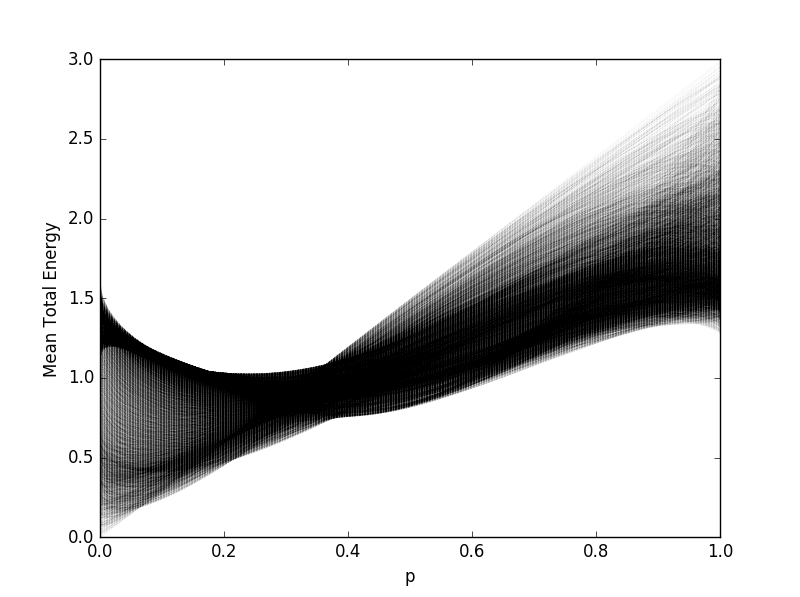
Figure 1: Mean total neural firing energy dynamics $\left\langle\hat{H}_{Net}\right\rangle_{l}$, for different values of $p$. In each case, 10000 iterations are plotted after initial 1000 iterations, which were dropped out for possible transients. The parameter $p$ proceeds in steps of $0.001$, starting at $p=0$ up until it reaches $1$.

A first point that can be noticed is that there are no visible periodic windows. On the other hand, the network seems to exhibit nonuniform behavior, namely, there are darker regions in the plot that correspond to concentrated fluctuations of the network for those values of $p$ and lighter regions that are less “explored”. This implies that the network may tend to show markers of turbulence for different values of $p$ associated with an asymmetric behavior. Figure 2 below illustrates this for a value of $p$ near 0.9. The fluctuations are concentrated in the region between 1.4J and 1.8J. Then, with less frequency there are those energy fluctuations above 2J, where the network is more active, the overall dynamics in figure 2 shows evidence of turbulence in the mean neural activation energy, illustrating figure 1’s profile for a specific value of $p$.

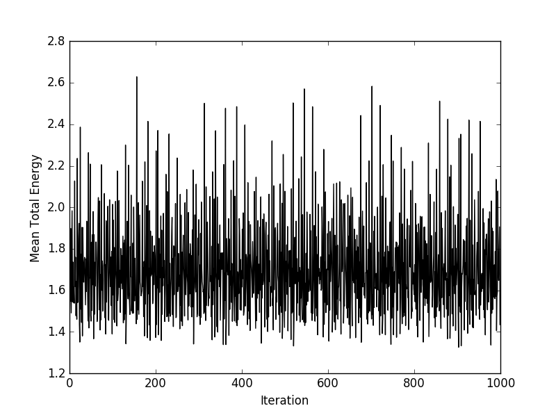
Figure 2: Mean total neural firing energy dynamics $\left\langle\hat{H}_{3}\right\rangle_{l}$, for 1000 iterations of the three-neuron neural network, with $p$ randomly chosen in the interval $[0,1]$, the value that $p$ obtained for this simulation was $0.8918547337153693$.

Another feature evident in figure 1 is that there is a transition in the dynamics profile. For lower values of $p$, the distribution for the mean total neural firing energy dynamics is asymmetric negative, that is, the deviations correspond to lower energy peaks. As $p$ approaches a region between 0.2 and 0.5, there is a bottleneck, where the dynamics becomes more uniformly distributed showing less dispersion of values. When $p$ rises further, the symmetry changes with the peaks corresponding to higher activation energy.

While the standard time series plot for $\left\langle\hat{H}_{3}\right\rangle_{l}$ allows us to picture the temporal evolution of the mean total energy. A delay embedding in three-dimensional space allows us to visualize, geometrically, possible emergent patterns for the mean energy, providing a geometric picture of the resulting emergent dynamics. In figure 3, we show the result of an embedding of the neural network’s mean total neural firing energy dynamics in three dimensional Euclidean space, for the same value of $p$ as in figure 2.

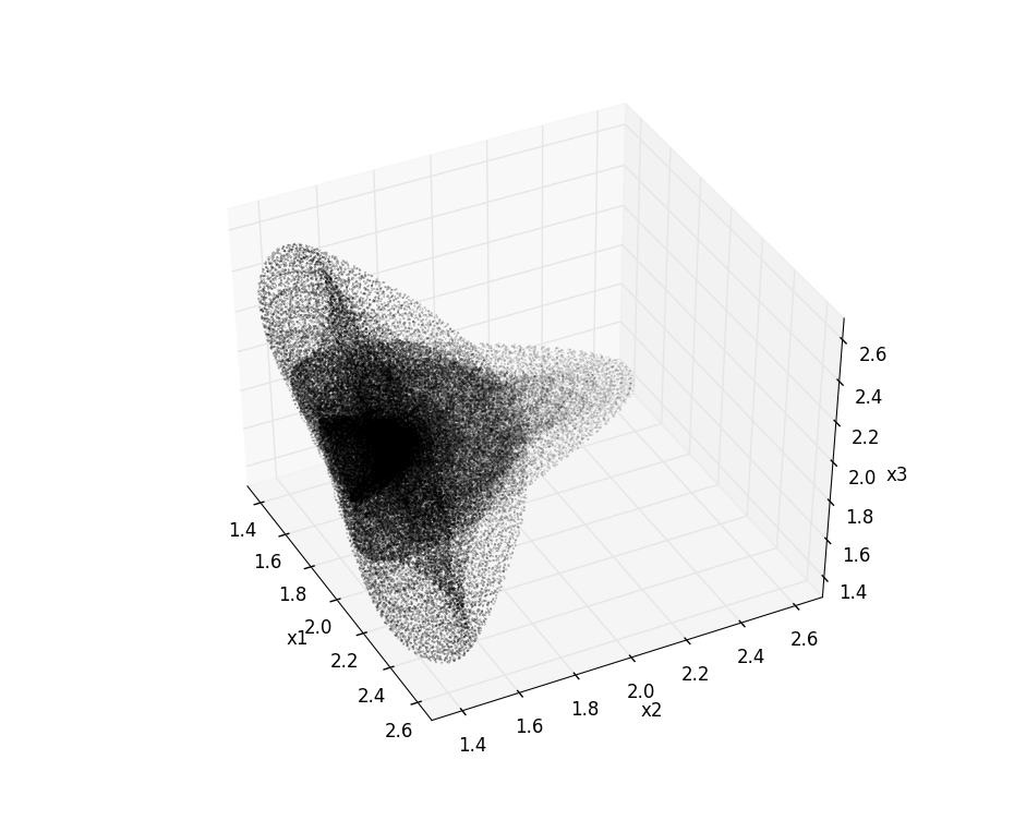
Figure 3: Delay coordinate embedding of the mean total neural firing energy dynamics for $p=0.8918547337153693$. For the time delay embedding we used a lag of 1 since this is the first zero crossing of the autocorrelation function, the embedding was obtained from $10^{5}$ iterations after 1000 initial iterations discarded for transients.

The embedded dynamics shows evidence of a complex structure. To address this structure we estimated first the correlation dimensions for different embedding dimensions. Table 1 in appendix shows the correlation dimensions estimated for four sequential epochs, each epoch containing 1000 embedded points. The estimates’ profiles are the same in the four epochs: for each embedding dimension, we get a statistically significant estimation, with an $R^{2}$ around 99% and there is a convergence to a correlation dimension between 4 and 5 dimensions, with a slowing down of the differences between each estimated correlation dimension, as the embedding dimension approximates the range from $d_{E}=6$ to $d_{E}=9$. In this range, $d_{E}=7$ has the lowest standard error.

Considering a delay embedding with $d_{E}=7$, table 2, in appendix, shows the estimated recurrence frequencies (expressed in percentage) calculated for each diagonal line of the distance matrix, for increasing radii, with the radii defined proportionally to the non-embedded sample series’ standard-deviation (in this case, a 5000 data points’ series).

The recurrence structure reveals that the mean energy dynamics has elements of dynamical stochasticity. Indeed, for radii between 0.5 and 0.7 standard-deviations the maximum percentage of diagonal line recurrence ranges from around 39% to around 89%, this means that the embedded trajectory is not periodic but there is at least one cycle with high recurrence (around 39%, in the case of 0.5 standard-deviations, around 68%, in the case of 0.6 standard-deviations, and around 89%, in the case of 0.7 standard-deviations). The mean cycle recurrence is, however, for this range of radii, very small, less that 1%, the median is 0% which means that half the diagonal lines have 0% recurrence and the other half have more than 0% recurrence, the standard-deviation of the recurrence percentage is also small.

Since, for a low radius, we do not have a full line with 100% recurrence, the dynamics, for the embedded sample trajectory, is not periodic. This profile changes as the radius is increased, indeed, as the radius is increased, a few number of diagonal lines with 100% recurrence start to appear, following a power law progression. For a radius of 2 standard-deviations we get 26 lines with 100% recurrence, we also get a median recurrence percentage of 4.1322% and a mean recurrence percentage of 8.8508%, wich means that the percentage of recurrence along the different cycles tends to be low.

The lines with 100% recurrence are not evenly separated, pointing towards an emergent quasiperiodic structure. The fact that a quasiperiodic recurrence pattern only appears for a rising radius, and the low (on average) recurrence indicates that the system has an emergent stochastic dynamical component and, simultaneously, persistent recurrence signatures that are proper of quasiperiodic dynamics, intermixing dynamical stochasticity and persistent quasiperiodic recurrences.

This is illustrated in figure 4, where we show a recurrence plot for a radius of 2 standard-deviations $d_{E}=7$ and a simulation comprised of 10000 data points. In the recurrence plot, we see the predominance of almost isolated dots typical of noise data, broken diagonal lines indicating unstable cycles typical of unstable divergence that takes place in chaotic dynamics, and the long full diagonal lines with 100% recurrence and unneven spacing, which is typical of quasiperiodic recurrences.

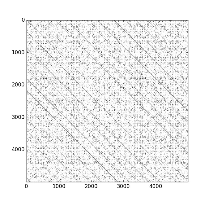
Figure 4: Recurrence plot for the table 2 data, with the radius of 2 standard-deviations, the embedded trajectory pairs with $\left\|\mathbf{x}_{u}-\mathbf{x}_{u^{\prime}}\right\|<\delta$ are marked in black, the other points are marked in white. The diagram’s orientation is from top to bottom and left to right, following the structure of the distance matrix.

In computer science and complex systems science, the dynamical regime that most closely matches the above dynamics is captured by the concept of edge of chaos, where stochastic dynamics and persistent regular dynamics coexist, expanding the systems’ adaptive ability due to a self-organization in an intermediate region between regular and stochastic dynamics (Kauffman and Johnsen, 1991; Kauffman, 1993). The intermixing of stochasticity and regular dynamics, as addressed above, show up as the radius is increased, indeed, for a low radius, the dynamics only shows noisy recurrences, as the radius is increased, however, resilient quasiperiodic recurrences, in the form of unevenly spaced diagonal lines with 100% recurrence, start to appear in the recurrence structure of the embedded series, following a power-law progression.

The quasiperiodic recurrences constitute, in this case, a form of noise resilient dynamical record, which may have possible applications in quantum technologies, namely in regards to the ability for a networked open quantum system to dynamically encode patterns in resilient recurrences. Table 3, in appendix, illustrates the level of resilience associated to the quasiperiodic recurrences. For that table, we divided 100000 iterations of the network into five epochs of 10000 iterations each and calculated the diagonal line recurrences on the delay-embedded series using a fixed radius of $\delta=0.4$ (slightly below 1.7 standard-deviations) and an embedding dimension of 7.

On average, the diagonal line recurrence frequencies are low for each epoch (around 4.3%) with a standard-deviation around 9.8%, which confirms the presence of dynamical stochasticity with a high dispersion around the mean. We identified, however, a fixed number of 28 diagonal lines with 100% recurrence that remain the same for each epoch, and represent 0.5607% of the total number of diagonal lines. The lowest period with 100% recurrence is 157, and the highest is 9871.

As shown in table 3, the observed distances between cycles ranges from 2 to 1111 embedded points, which shows the unevenness of the distances between the 100% recurrence lines, typical of quasiperiodic dynamics. The mean distance between the lines with 100% recurrence is 359.778.

Table 4, in appendix, shows the distribution of distances between the diagonal lines. There are two dominant distances which represent roughly 51.85% of the distribution: 157 (which occurs 9 times) and 389 (which occurs 5 times), besides these two main dominant distances, we get a uniform distribution on the distances 26, 131, 363, 562, 722 and 1111, and an adicional single case of a distance equal to 520. The fact that there is no third dominant distance, as occurs for a standard quasiperiodic motion on a torus (Zou, 2007), and the uniform distribution over an unneven set of distances representing about 44.44% of the distance distribution indicates a form of emergent erratic quasiperiodicity, present at that radius.

We can trace back the interplay between dynamical stochasticity and emergent persistent quasiperiodicity, present in the mean total neural firing energy dynamics, to the network’s cognition of the environment. Indeed, in this case, since the environment is an ensemble in a maximum (von Neumann) entropy distribution over the eigenstates $\left|\varepsilon_{k}\right\rangle\left\langle\varepsilon_{k}\right|$, the final dynamics results from the mixture over the different neural activation orders.

If we consider the processing of each environment’s eigenstate by the network, then, we can identify the differences in the network’s dynamics which contribute to the final emergent pattern identified above. For instance, for the environment’s state $\left|\varepsilon_{1}\right\rangle\left\langle\varepsilon_{1}\right|$, we obtain a more regular attractor structure (figure 5, left) than for the environment’s state $\left|\varepsilon_{5}\right\rangle\left\langle\varepsilon_{5}\right|$ (figure 5, right).

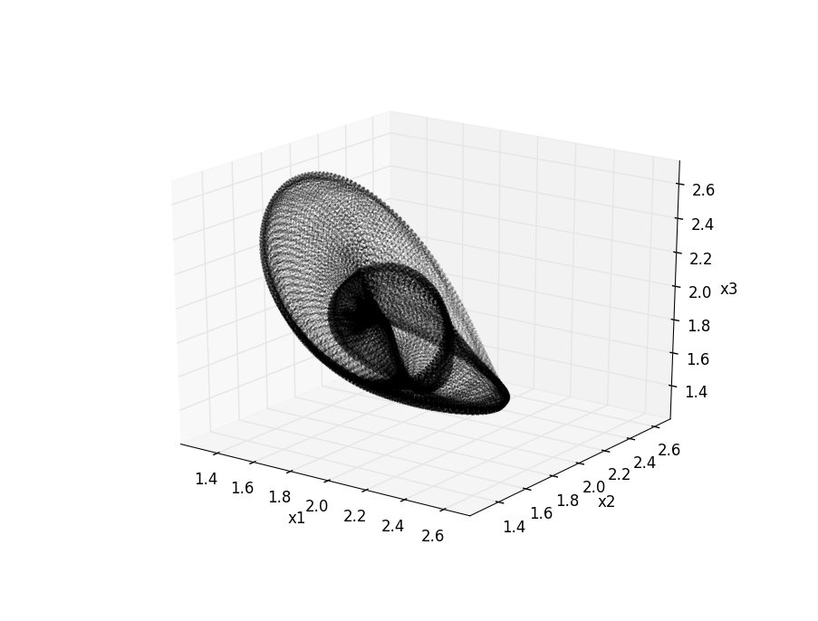
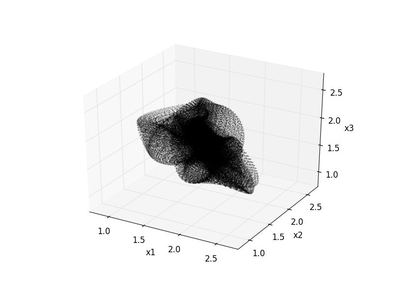
Figure 5: Delay coordinate embedding of the mean total neural firing energy dynamics for $p=0.8918547337153693$, with the environment’s initial state set to the basis state $\left|\varepsilon_{1}\right\rangle\left\langle\varepsilon_{1}\right|$ (left) and in the basis state $\left|\varepsilon_{5}\right\rangle\left\langle\varepsilon_{5}\right|$ (right). For the time delay embedding, we used a lag of 1 since this is the first zero crossing of the autocorrelation function, the embedding was obtained from 100000 iterations after 1000 initial iterations discarded for transients.

Table 5, in appendix, illustrates the recurrences obtained for each environment’s eigenstate using, for comparison purposes, a seven dimensional delay embeding of 10000 iterations of the network, and defining a radius $\delta=0.4$. From table 5, it follows that the dynamics depends critically on the feedforward and backpropagation neural processing triggered by the environment. Indeed, there are more regular dynamics triggered, respectively, by the network’s processing of the environment in the states $\left|\varepsilon_{1}\right\rangle\left\langle\varepsilon_{1}\right|$ and $\left|\varepsilon_{6}\right\rangle\left\langle\varepsilon_{6}\right|$, leading, in both cases, to a total number of 105 diagonal lines with 100% recurrence, and a mean recurrence around 2.5%.

In the network’s processing of the environment in the state $\left|\varepsilon_{1}\right\rangle\left\langle\varepsilon_{1}\right|$, there is first a feedforward activation, where $N_{1}$’s state is transformed conditionally on $N_{2}$ and $N_{3}$’s states, then, there is a sequence of two backpropagation transformations from $N_{1}$ to $N_{2}$ (completing the recurrent loop) and to $N_{3}$ (completing the second recurrent loop), where $N_{3}$’s state is transformed conditionally on $N_{1}$ (recurrent activation) and on $N_{2}$ (which, in this case, is a feedforward activation).

In the case of the network’s processing of the environment state $\left|\varepsilon_{6}\right\rangle\left\langle\varepsilon_{6}\right|$, there are two feedforward transformations: the transformation of $N_{3}$’s state, conditional on the other two neurons, then, there is a second feedforward activation where $N_{2}$’s state is transformed conditionally on $N_{1}$. After these two feedforward activations there is a backpropagation from $N_{2}$ and $N_{3}$ to the neuron $N_{1}$ closing the recurrent loops. The element in common to the neural processing of the states $\left|\varepsilon_{1}\right\rangle\left\langle\varepsilon_{1}\right|$ and $\left|\varepsilon_{6}\right\rangle\left\langle\varepsilon_{6}\right|$ is the second transformation which is, in both cases, $N_{1}\rightarrow N_{2}$.

A similar pattern is present in the other dynamical profiles. Thus, the neural processing of the states $\left|\varepsilon_{2}\right\rangle\left\langle\varepsilon_{2}\right|$ and $\left|\varepsilon_{4}\right\rangle\left\langle\varepsilon_{4}\right|$ lead to the lowest recurrence, for those embedding parameters, with 6 and 7 diagonal lines with 100% recurrence, and a mean recurrence around 0.57%, furthermore, the diagonal lines with 100% recurrence are less resilient with divergence occurring for repeated simulations in sequential epochs of size 10000. These two low recurrence dynamics are also characterized by the same second neural activation.

Indeed, the neural processing of the environment in the state $\left|\varepsilon_{2}\right\rangle\left\langle\varepsilon_{2}\right|$ is such that the feedforward transformation $N_{2}\rightarrow N_{1}\leftarrow N_{3}$ is activated first, then, follows the activation of the neural circuit $N_{1}\rightarrow N_{3}\leftarrow N_{2}$, where $N_{1}$ is feeding backward (backpropagation) to $N_{3}$ and $N_{2}$ is feeding forward to $N_{3}$, finally there is a feeding backward from $N_{1}$ to $N_{2}$.

Similarly, the neural processing of the environment in the state $\left|\varepsilon_{4}\right\rangle\left\langle\varepsilon_{4}\right|$, is such that $N_{1}$ first feeds forward to $N_{2}$, and then both neurons feed forward to $N_{3}$ (following the circuit $N_{1}\rightarrow N_{3}\leftarrow N_{2}$), and then $N_{2}$ and $N_{3}$ feed backward to $N_{1}$.

The third pair of dynamics comes from the neural processing of the environment in the states $\left|\varepsilon_{3}\right\rangle\left\langle\varepsilon_{3}\right|$ and $\left|\varepsilon_{5}\right\rangle\left\langle\varepsilon_{5}\right|$. Again, the second transformation coincides. Indeed, when the environment is in the state $\left|\varepsilon_{3}\right\rangle\left\langle\varepsilon_{3}\right|$, the neural network first activates the feedforward connection $N_{1}\rightarrow N_{2}$, then the neural circuit $N_{2}\rightarrow N_{1}\leftarrow N_{3}$ is activated, where $N_{2}$ is feeding backward to $N_{1}$ and $N_{3}$ is feeding forward to $N_{1}$, after this transformation the final neural circuit $N_{1}\rightarrow N_{3}\leftarrow N_{2}$ is activated, where $N_{1}$ feeds backward to $N_{3}$ and $N_{2}$ feeds forward to $N_{3}$. When the environment is in the state $\left|\varepsilon_{5}\right\rangle\left\langle\varepsilon_{5}\right|$, the feedforward direction is $N_{1}\rightarrow N_{3}\leftarrow N_{2}$, followed by the neural circuit $N_{2}\rightarrow N_{1}\leftarrow N_{3}$ activation, where $N_{3}$ is feeding backward to $N_{1}$ and $N_{2}$ is feeding forward, finally there is a last transformation where $N_{1}$ feeds backward to $N_{2}$.

In both of these cases we, again, have the same second transformation, the number of lines with 100% recurrence obtained are equal to 10 and the mean recurrence is around 1%.

This shows how the relation between the way in which information flows in the network in its processing of the environment can have an effect on the network’s dynamics. Besides the initial state of the environment, the initial state of the network also matters. The above examples were worked from $p$ in the region of values above the bottleneck shown in figure 1.

If the value of $p$ is lowered, then, the quasiperiodic order becomes more significant even though there is always a strong presence of stochastic dynamics, so that for lower values of $p$ we get emergent torus-shaped attractors, as is shown in figure 6’s example.

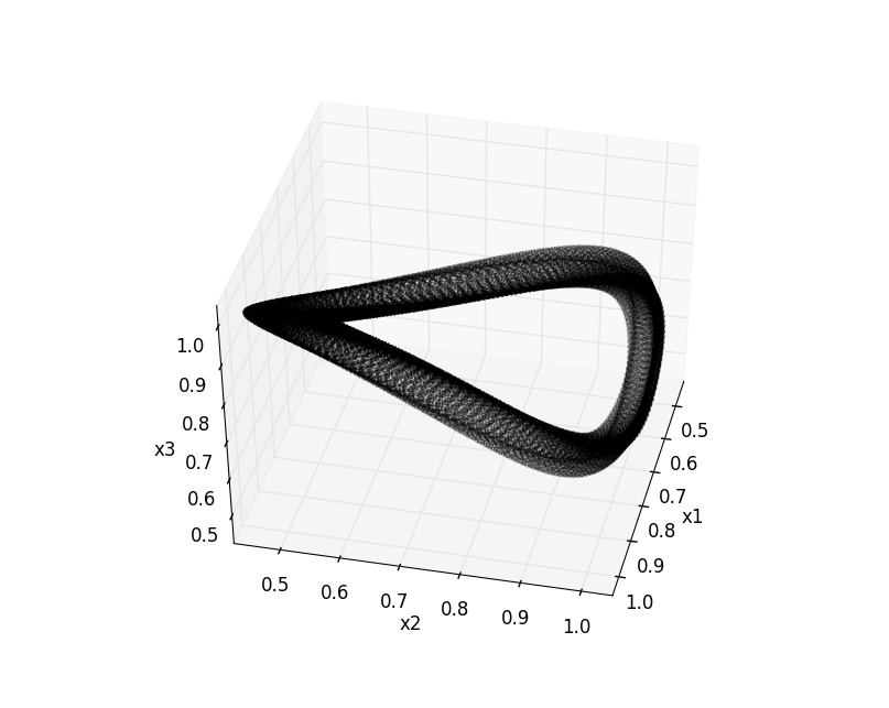
Figure 6: Delay coordinate embedding of the mean total neural firing energy dynamics, with $p=0.19232544805500018$. For the time delay embedding we used a lag of 1 since this is the first zero crossing of the autocorrelation function, the embedding was obtained from 100000 iterations after 1000 initial iterations discarded for transients, the initial state is described by Eq.(73).

In figure 7, we plot the conditional probabilities of getting a 100% recurrence line from a random selection of lines with recurrence points (these correspond to the probabilities $P\left[\left.C_{d_{E},\delta,\theta}=1\right|C_{d_{E},\delta,\theta}>0\right]$ defined in Eq.(69)), using a radius of 1 standard-deviation, for different values of $p$ and different embedding dimensions and for cycle lengths from an original series of 2000 data points (thus, we get the probability of 100% recurrence, given that the line shows recurrence for low period cycles).

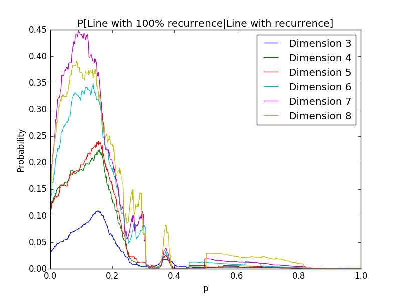
Figure 7: Probability of 100% recurrence diagonal line given that the line contains recurrence points, for the mean total neural firing energy dynamics $\left\langle\hat{H}_{3}\right\rangle_{l}$, applying a delay embedding on a 2000 iterations’ simulation of the network, after initial 1000 iterations dropped for transients. The parameter $p$ proceeds in steps of $0.001$, starting at $p=0$ up until it reaches $1$, the embedding dimensions range from 3 to 8 and the delay period is in each case set as the first zero crossing of the autocorrelation function. The radius $\delta$ was set to 1 standard-deviation

For all cases, shown in figure 7, the probability is less than 1, which means that the system always exhibits a combination of stochastic dynamics and quasiperiodic recurrences, however, the probability of finding 100% recurrence lines in a random selection of lines with recurrent points, for an open neighborhood size of 1 standard-deviation, increases for a region of $p$ that goes from below 0.1 up to 0.2 and then again, although with lower values, around 0.3 and 0.4 (which includes the bottleneck region). In these cases we get emergent toroidal attractors with evidence of noisy quasiperiodic dynamics. These regions are the ones in which the network produces a more resilient quasiperiodic dynamics.

As $p$ is raised, the quasiperiodicity tends to be less representative and the network tends progressively to a form of emergent stochastic dynamics. Even though, for high value of $p$, as we showed above, we still get edge of chaos-like dynamical markers, the level of proximity to a stochastic dynamics increases with the initial amplitude associated with each neuron’s active firing state, the higher this amplitude is, the more the network tends to a predominantely stochastic dynamics.

4 Conclusion

As models of networked quantum computation, QuANNs introduce novel features for both quantum computer science as well as for machine learning in general. While a QuANN can be designed such that a certain computational problem is solved by parallel networked quantum processors, the main purpose of a QuANN, as a computational system, is to go beyond a programmed networked quantum computer.

Namely, a QuANN should work as an artificial cognitive system that is capable of evaluating the task with respect to a certain computational goal and select accordingly the best quantum circuits to implement that allow it to solve the problem efficiently.

The first part of the present work was aimed at the implementation of this type of quantum neural cognition, using a feedforwad neural network structure with quantum backpropagation. In this case, the output neurons take on the task of evaluating the input firing patterns with respect to the intended task, this is the first stage of the neural processing dynamics, where the network’s computation tends, during the neural learning temporal interval, towards a quantum circuit that is adapted to the computational problem. The second stage of the task (the backpropagation stage) is to conditionally transform the input layer’s state so as to solve the problem.

The quantum backpropagation effectively implements a form of adaptive error correction, in the sense that the input layer’s state is conditionally transformed in such a way that it exhibits the firing patterns that solve the computational problem. This is illustrated in both examples provided in section 2, where, for the first problem (subsection 2.1), the network adaptively transforms the input layer so that it exhibits a specific firing pattern, and, for the second problem, the network adaptively transforms the input layer so that it represents a general n-to-m Boolean function, exemplifying the application of the neural learning scheme to a computer science problem. The first problem shows how the quantum network can adaptively set the energy levels of each neuron in a layer, an ability that may be relevant for future quantum networked technologies, namely, in what regards the ability of quantum networks to self-manage energy levels.

While the framework, addressed in section 2, introduces a quantum neural learning scheme to adaptively solve specific computational problems, in section 3, the feedforward and backpropagation take on a role as building blocks for an unsupervised dynamical neural processing of an environment, with the conditional neural state transition taking place with respect to the different neural activation orders, thus extending the formalism of quantum computation with changing orders of gates (Procopio, et al., 2015; Brukner, 2014; Chiribella, et al., 2013; Aharonov, et al., 1990) to the context of quantum machine learning.

The example shown in section 3, recovers, in a quantum setting, specific features that have been addressed in classical Hopfield networks and classical models of neural computation, namely the relation with chaos as a way to extend the memory capacity of neural networks in learning new patterns (Watanabe et al., 1997; Akhmet and Fen, 2014) as well as the ability of ANNs to simulate neural synchronization and adaptive dynamics taking advantage of a transition between chaos and quasiperiodic recurrences (Akhmet and Fen, 2014).

In the network simulated in section 3, we get a simultaneous presence of two levels of emergent dynamics: a stochastic dynamics and a resilient quasiperiodic dynamics, evident in the recurrence statistics. The higher the initial amplitude for each neuron to be in the active state, the stronger the stochastic dynamics is, with the recurrence patterns showing markers of stochastic noise-like dynamics, however, with a sufficiently high radius used for the neighborhood structure analysis, resilient quasiperiodic recurrences start to appear, so that the network’s mean neural firing energy dynamics exhibits a coexistence of stochastic dynamics and resilient quasiperiodic dynamics.

The quasiperiodic dynamics becomes more dominant when the initial amplitude for each neuron to be in the nonfiring state is high, for these values toroidal attractors appear, although there is still evidence of the presence of stochastic dynamics.

The network exhibits, thus, a self-organization towards a dynamical regime where it is able to sustain a persistent order alongside stochastic dynamics, intermixing both randomness and resilient quasiperiodic dynamical patterns that constitute a form of noise resilient dynamical record. The dynamical markers are typical of the concept of edge of chaos. At the edge of chaos, a complex adaptive system is simultaneously capable of change and structure conservation, producing the order it needs to survive, maximizing its adaptability since it neither falls into a rigid unchanging structure (ceasing to adapt) nor falls into the opposite chaotic side leading to a collapse of conserved structures (Packard, 1988; Langton, 1990; Crutchfield and Young, 1990; Kauffman and Johnsen, 1991; Kauffman, 1993). Future work on QuANN dynamics is needed in order to produce a theory of open system’s quantum cognition in the context of quantum machine learning research, in particular in what regards forms of distributed system-wide awareness in large QuANNs and dynamical memory formation.

Aharonov Y, Anandan J, Popescu S and Vaidman L. Superpositions of time evolutions of a quantum system and a quantum time-translation machine. Phys. Rev. Lett. 1990; 64(25):2965-2968.

Akhmet M and Fen MO. Generation of cyclic/toroidal chaos by Hopfield neural networks. Neurocomputing, 2014; 145:230-239.

Behrman EC, Niemel J, Steck JE, Skinner SR. A Quantum Dot Neural Network, In: T. Toffoli T and M. Biafore, Proceedings of the 4th Workshop on Physics of Computation, Elsevier Science Publishers, Amsterdam, 1996; 22-24.

Bertschinger N and Natschläger T. Real-time computation at the edge of chaos in recurrent neural networks. Neural Comput., 2004; 16(7):1413-36.

Brukner Č. Quantum causality. Nature Physics, 2014; 10:259-263.

Chiribella G, D’Ariano GM, Perinotti P and Valiron B. Quantum computations without definite causal structure. Phys. Rev. A, 2013; 88(2):022318.

Chrisley R. Quantum learning, In: Pylkkänen P and Pylkkö P (eds.), New directions in cognitive science: Proceedings of the international symposium, Saariselka, 4-9 August, Lapland, Finland, Finnish Artificial Intelligence Society, Helsinki, 1995; 77-89.

Crutchfield JP and Young K. Computation at the Onset of Chaos, In: Zurek W. Entropy, Complexity, and the Physics of Information. SFI Studies in the Sciences of Complexity. Proceedings Volume VIII in the Sante Fe Institute Studies in the Sciences of Complexity, Addison-Wesley, Reading, Massachusetts, 1990; 223-269.

Gonçalves CP. Quantum Cybernetics and Complex Quantum Systems Science - A Quantum Connectionist Exploration. NeuroQuantology, 2015a; 13(1): 35-48.

Gonçalves CP. Financial Market Modeling with Quantum Neural Networks. Review of Business and Economics Studies, 2015b; 3(4):44-63.

Gorodkin J, Sørensen A and Winther O. Neural Networks and Cellular Automata Complexity. Complex Systems, 1993, 7:1-23.

Grassberger P and Proccacia I. Characterization of strange attractors. Phys. Rev. Lett, 1983a; 50:346-349.

Grassberger P and Proccacia I. Measuring the Strangeness of Strange Attractors. Physica D, 1983b; 9:189-208.

Haake F, Kuś M and Scharf R. Classical and Quantum Chaos for a Kicked Top. Z. Phys. B. - Condensed Matter, 1987; 65:381-395.

Ivancevic VG and Ivancevic TT. Quantum Neural Computation, Springer, Dordrecht, 2010.

Kak S. Quantum Neural Computing. Advances in Imaging and Electron Physics, 1995; 94:259-313.

Kaplan D and Glass L. Understanding Nonlinear Dynamics. Springer, New York, 1995.

Kauffman SA and Johnsen S. Coevolution to the Edge of Chaos: Coupled Fitness Landscapes, Poised States, and Coevolutionary Avalanches. J. theor. Biol., 1991; 149:467-505.

Kauffman SA. The Origins of Order: Self-Organization and Selection in Evolution. Oxford University Press, New York, 1993.

Langton C. Computation at the Edge of Chaos: Phase Transitions and Emergent Computation. Physica D, 1990; 42:12-37.

Menneer T and Narayanan A. Quantum-inspired Neural Networks, technical report R329, Department of Computer Science, University of Exeter, Exeter, United Kingdom, 1995.

Menneer T Quantum Artificial Neural Networks, Ph. D. thesis, The University of Exeter, UK, 1998.

Nayfeh, AH and Balachandran, B. Applied Nonlinear Dynamics - Analytical, Computational and Experimental Methods, Wiley-VCH, Germany, 2004.

Packard, NH. Adaptation toward the edge of chaos. University of Illinois at Urbana-Champaign, Center for Complex Systems Research, 1988.

Procopio LM, Moqanaki A, Araújo M, Costa F, Calafell IA, Dowd EG, Hamel DR, Rozema LA, Brukner Č and Walther P. Experimental superposition of orders of quantum gates. Nature Communications, 2015; 6:7913.

Schuld M, Sinayskiy I and Petruccione F. The quest for a Quantum Neural Network. Quantum Information Processing, 2014a; 13(11): 2567-2586.

Schuld M, Sinayskiy I and Petruccione F. Quantum walks on graphs representing the firing patterns of a quantum neural network. Phys. Rev. A, 2014b; 89: 032333.

Watanabe M, Aihara K and Kondo S. Self-organization dynamics in chaotic neural networks. Control Chaos Math. Model., 1997; 8:320-333

Wolfram S. A New Kind of Science. Wolfram Research, Canada, 2002.

Zou Y. Exploring Recurrences in Quasiperiodic Dynamical Systems. Ph. D. Thesis, University of Potsdam, 2007.

Appendices - Tables

$d_{E}$	Epoch 1	Epoch 2	Epoch 3	Epoch 4
3	$\begin{array}[]{c}D_{2}\simeq 2.1051\\ R^{2}\simeq 0.9992\\ sig.\simeq 2.35e-07\\ S.E.\simeq 0.0296\end{array}$	$\begin{array}[]{c}D_{2}\simeq 2.1295\\ R^{2}\simeq 0.9992\\ sig.\simeq 2.35e-07\\ S.E.\simeq 0.0300\end{array}$	$\begin{array}[]{c}D_{2}\simeq 2.1001\\ R^{2}\simeq 0.9991\\ sig.\simeq 3.24e-07\\ S.E.\simeq 0.0321\end{array}$	$\begin{array}[]{c}D_{2}\simeq 2.1230\\ R^{2}\simeq 0.9990\\ sig.\simeq 3.92e-07\\ S.E.\simeq 0.0340\end{array}$
4	$\begin{array}[]{c}D_{2}\simeq 2.8127\\ R^{2}\simeq 0.9991\\ sig.\simeq 2.75e-07\\ S.E.\simeq 0.0412\end{array}$	$\begin{array}[]{c}D_{2}\simeq 2.8327\\ R^{2}\simeq 0.9993\\ sig.\simeq 1.61e-07\\ S.E.\simeq 0.0363\end{array}$	$\begin{array}[]{c}D_{2}\simeq 2.7935\\ R^{2}\simeq 0.9990\\ sig.\simeq 3.89e-07\\ S.E.\simeq 0.0363\end{array}$	$\begin{array}[]{c}D_{2}\simeq 2.8550\\ R^{2}\simeq 0.9989\\ sig.\simeq 4.69e-07\\ S.E.\simeq 0.0478\end{array}$
5	$\begin{array}[]{c}D_{2}\simeq 3.5127\\ R^{2}\simeq 0.9992\\ sig.\simeq 2.15e-07\\ S.E.\simeq 0.0483\end{array}$	$\begin{array}[]{c}D_{2}\simeq 3.5111\\ R^{2}\simeq 0.9995\\ sig.\simeq 8.36e-08\\ S.E.\simeq 0.0382\end{array}$	$\begin{array}[]{c}D_{2}\simeq 3.4820\\ R^{2}\simeq 0.9991\\ sig.\simeq 2.74e-07\\ S.E.\simeq 0.0509\end{array}$	$\begin{array}[]{c}D_{2}\simeq 3.5544\\ R^{2}\simeq 0.9992\\ sig.\simeq 2.55e-07\\ S.E.\simeq 0.0511\end{array}$
6	$\begin{array}[]{c}D_{2}\simeq 4.0670\\ R^{2}\simeq 0.9996\\ sig.\simeq 5.69e-08\\ S.E.\simeq 0.0401\end{array}$	$\begin{array}[]{c}D_{2}\simeq 4.0916\\ R^{2}\simeq 0.9998\\ sig.\simeq 1.51e-08\\ S.E.\simeq 0.0290\end{array}$	$\begin{array}[]{c}D_{2}\simeq 4.0690\\ R^{2}\simeq 0.9997\\ sig.\simeq 3.43e-08\\ S.E.\simeq 0.0354\end{array}$	$\begin{array}[]{c}D_{2}\simeq 4.1488\\ R^{2}\simeq 0.9998\\ sig.\simeq 1.40e-08\\ S.E.\simeq 0.0354\end{array}$
7	$\begin{array}[]{c}D_{2}\simeq 4.4239\\ R^{2}\simeq 0.9999\\ sig.\simeq 1.23e-09\\ S.E.\simeq 0.0168\end{array}$	$\begin{array}[]{c}D_{2}\simeq 4.4417\\ R^{2}\simeq 0.9999\\ sig.\simeq 1.73e-09\\ S.E.\simeq 0.0182\end{array}$	$\begin{array}[]{c}D_{2}\simeq 4.4001\\ R^{2}\simeq 0.9997\\ sig.\simeq 2.70e-08\\ S.E.\simeq 0.0360\end{array}$	$\begin{array}[]{c}D_{2}\simeq 4.4438\\ R^{2}\simeq 0.9998\\ sig.\simeq 1.13e-08\\ S.E.\simeq 0.0293\end{array}$
8	$\begin{array}[]{c}D_{2}\simeq 4.5664\\ R^{2}\simeq 0.9999\\ sig.\simeq 5.07e-09\\ S.E.\simeq 0.0246\end{array}$	$\begin{array}[]{c}D_{2}\simeq 4.4989\\ R^{2}\simeq 0.9999\\ sig.\simeq 4.06e-07\\ S.E.\simeq 0.0726\end{array}$	$\begin{array}[]{c}D_{2}\simeq 4.4183\\ R^{2}\simeq 0.9981\\ sig.\simeq 1.32e-06\\ S.E.\simeq 0.0958\end{array}$	$\begin{array}[]{c}D_{2}\simeq 4.4756\\ R^{2}\simeq 0.9983\\ sig.\simeq 1.04e-06\\ S.E.\simeq 0.0914\end{array}$
9	$\begin{array}[]{c}D_{2}\simeq 4.300\\ R^{2}\simeq 0.9986\\ sig.\simeq 7.84e-06\\ S.E.\simeq 0.0818\end{array}$	$\begin{array}[]{c}D_{2}\simeq 4.2369\\ R^{2}\simeq 0.9964\\ sig.\simeq 4.92e-06\\ S.E.\simeq 0.1277\end{array}$	$\begin{array}[]{c}D_{2}\simeq 4.0665\\ R^{2}\simeq 0.9953\\ sig.\simeq 8.15e-06\\ S.E.\simeq 0.1391\end{array}$	$\begin{array}[]{c}D_{2}\simeq 4.2330\\ R^{2}\simeq 0.9961\\ sig.\simeq 5.71e-06\\ S.E.\simeq 0.1324\end{array}$

?tablename? 1: Correlation dimensions estimated for four epochs of 1000 embedded points each, the epochs were obtained after 1000 iterations initially dropped for transients, with $p=0.8918547337153693$, and a lag of 1. In each case, the radius ranges in the region of power-law scaling, between 1 sample standard-deviation up to 1.7 sample standard-deviations, with steps of 0.1 standard-deviations.

$\delta/\sigma$	Max	Min	Mean	Median	Std. Dev.	#Lines (100% Rec.)
0.5	39.6761%	0%	0.0217%	0%	0.6161%	0
0.6	68.6640%	0%	0.0557%	0%	1.2144%	0
0.7	89.9595%	0%	0.1099%	0%	1.8920%	0
0.8	100%	0%	0.1951%	0%	2.7087%	1
0.9	100%	0%	0.3224%	0%	3.6264%	1
1	100%	0%	0.4885%	0%	4.2603%	3
1.1	100%	0%	0.7173%	0.0497%	4.8634%	5
1.2	100%	0%	1.0312%	0.1285%	5.5636%	5
1.3	100%	0%	1.4541%	0.2553%	6.3387%	6
1.4	100%	0%	2.0026%	0.4564%	7.1779%	7
1.5	100%	0%	2.6985%	0.7475%	8.0889%	9
1.6	100%	0%	3.5636%	1.1313%	9.0840%	12
1.7	100%	0%	4.5100%	1.6380%	10.1223%	14
1.8	100%	0%	5.8131%	2.2629%	11.1719%	17
1.9	100%	0%	7.2334%	3.0865%	12.2404%	21
2	100%	0%	8.8508%	4.1322%	13.3660%	26

?tablename? 2: Recurrence frequencies calculated for the three neuron neural network, the frequencies were calculated for a delay embedding with $d_{E}=7$ for a 5000 iterations series taken from a 6000 iterations simulation, with the first 1000 iterations removed for transients and $p=0.8918547337153693$. The radii presented were obtained from the standard-deviation of the original series ranging from 0.5 standard deviations to up to 2 standard-deviations in steps of 0.1 standard-deviations.

Epoch	Mean	Median	Std. Dev.
E1	4.2885	1.5046	9.8745
E2	4.2868	1.4957	9.8370
E3	4.2832	1.5021	9.8236
E4	4.3016	1.5035	9.8620
E5	4.3052	1.5094	9.8470
E6	4.2830	1.5038	9.8607
E7	4.3096	1.5006	9.8459
E8	4.2967	1.5062	9.8299
E9	4.2680	1.4858	9.8475
E10	4.3235	1.5038	9.8846
Lines with 100% Recurrence Statistics
# Lines with 100% recurrence			28
% Lines with 100% recurrence			0.5607%
Min Period			157
Max Period			9871
Min Distance			2
Max Distance			1111
Mean Distance			359.778

?tablename? 3: Diagonal line recurrence statistics for 10 sequential epochs’ division of 100000 iterations of the neural network, with 10000 mean total firing energy data points for each epoch size. The statistics were calculated for a delay embedding of each epoch’s data using $d_{E}=7$ and $\delta=0.4$, and $p=0.8918547337153693$.

Distance	Frequency
26	2
131	2
157	9
363	2
389	5
520	1
565	2
722	2
1111	2
Total	27

?tablename? 4: Distance distribution for the 100% recurrence lines identified in the previous table’s simulations.

Environment	Permutations	# Lines	Mean Rec.
$\left|\varepsilon_{1}\right\rangle\left\langle\varepsilon_{1}\right|$	$\hat{L}_{3}\hat{L}_{2}\hat{L}_{1}$	105	2.4952%
$\left|\varepsilon_{2}\right\rangle\left\langle\varepsilon_{2}\right|$	$\hat{L}_{2}\hat{L}_{3}\hat{L}_{1}$	6	0.5670%
$\left|\varepsilon_{3}\right\rangle\left\langle\varepsilon_{3}\right|$	$\hat{L}_{3}\hat{L}_{1}\hat{L}_{2}$	10	1.0225%
$\left|\varepsilon_{4}\right\rangle\left\langle\varepsilon_{4}\right|$	$\hat{L}_{1}\hat{L}_{3}\hat{L}_{2}$	7	0.5703%
$\left|\varepsilon_{5}\right\rangle\left\langle\varepsilon_{5}\right|$	$\hat{L}_{2}\hat{L}_{1}\hat{L}_{3}$	10	1.0249%
$\left|\varepsilon_{6}\right\rangle\left\langle\varepsilon_{6}\right|$	$\hat{L}_{1}\hat{L}_{2}\hat{L}_{3}$	105	2.4996%

?tablename? 5: Number of lines with 100% recurrence and mean recurrence, for different initial states of the environment, the data comes from a delay embedding for a simulation of 10000 iterations using $d_{E}=7$, $\delta=0.4$, and $p=0.8918547337153693$.