Constraints on galaxy formation models from the galaxy stellar mass function and its evolution

Abstract

We explore the parameter space of the semi-analytic galaxy formation model galform, studying the constraints imposed by measurements of the galaxy stellar mass function (GSMF) and its evolution. We use the Bayesian Emulator method to quickly eliminate vast implausible volumes of the parameter space and zoom in on the most interesting regions, allowing us to identify a set of models that match the observational data within model uncertainties. We find that the GSMF strongly constrains parameters related to quiescent star formation in discs, stellar and AGN feedback and threshold for disc instabilities, but weakly restricts other parameters. Constraining the model using local data alone does not usually select models that match the evolution of the GSMF well. Nevertheless, we show that a small subset of models provides acceptable match to GSMF data out to redshift 1.5. We explore the physical significance of the parameters of these models, in particular exploring whether the model provides a better description if the mass loading of the galactic winds generated by starbursts ($\beta_{0,\text{burst}}$) and quiescent disks ($\beta_{0,\text{disc}}$) is different. Performing a principal component analysis of the plausible volume of the parameter space, we write a set of relations between parameters obeyed by plausible models with respect to GSMF evolution. We find that while $\beta_{0,\text{disc}}$ is strongly constrained by GSMF evolution data, constraints on $\beta_{0,\text{burst}}$ are weak. Although it is possible to find plausible models for which $\beta_{0,\text{burst}}=\beta_{0,\text{disc}}$, most plausible models have $\beta_{0,\text{burst}}>\beta_{0,\text{disc}}$, implying – for these – larger SN feedback efficiency at higher redshifts.

1 Introduction

Semi-analytic models of galaxy formation (SAMs) are well established tools for exploring galaxy formation scenarios in their cosmological context. The problem of how galaxies form and evolve is described by a set of coupled differential equations dealing with well-defined astrophysical processes. These are driven by dark matter halo merger trees that determine the source terms in the equation network (for reviews see e.g. Benson, 2010; Baugh, 2006; Somerville & Davé, 2015). Due to the approximate nature of the methods used in these simulations, and the uncertainties in the physical process that are modelled, these models include a large number of uncertain parameters. While order of magnitude estimates for these parameters can be made, their precise values must be determined by comparison to observational data.

Traditionally, parameter values have been set through a trial-and-error approach, where the galaxy formation modeller varies an individual parameter developing intuition about its effects on the model predictions for a particular observable and then uses this understanding to select a parameter set that gives a good description of the observations. Despite its simplicity, and obvious limitations, this procedure has led to substantial progress in the field. Recently, however, several papers have employed more rigorous statistical methods to explore the high dimensional parameter space systematically (Kampakoglou et al., 2008; Henriques et al., 2009; Bower et al., 2010; Henriques et al., 2013; Benson, 2014; Lu et al., 2014; Henriques et al., 2015). Such approaches provide a richer analysis, and seek to identify the regions of parameter space that are in agreement with observational data, and not just to find optimal parameter values. This therefore informs as to the uniqueness of the parameter choices, and provides understanding of the degeneracies between different parameters.

In this work we study which constraints are imposed on the semi-analytic model galform by the observations of galaxy stellar mass function (GSMF). We first consider the constraints imposed by local observations and then investigate how the parameters are further constrained by the introduction of high redshift data. This makes powerful use of the iterative emulator technique described by Bower et al. (2010), which provides an efficient way of probing a high dimensional parameter space. Importantly, the method allows additional constraints to be added in post-processing. Thus, we start by finding the region in the parameter space which contains models that produce a good match to the local Universe GSMF. This region is, then, further probed to check whether a match to higher redshift data is possible. By analysing 2D projections of the plausible models sub-volume and performing a principal component analysis of it, we are able to study the degeneracies and interactions between the most constrained parameters. We note that typical approaches to analysing comparable models using Bayesian MCMC require millions of model runs (at least), while the approach used here, which utilises Bayesian emulation, only required tens of thousands of model runs, representing a substantial improvement in efficiency.

Closely reproducing the observed high-redshift galaxy mass function (Cirasuolo et al., 2010; Henriques et al., 2013) is problematic for many galaxy formation models. Henriques et al. (2013), for example, concludes that the effectiveness of galaxy feedback (specifically the re-incorporation time of expelled gas) must depend on the virial mass of the dark matter halo on the basis of a Monte Carlo exploration of the parameter space of their model. This is not fully satisfactory, however, since one would expect the re-incorporation time to be physically related to the halo dynamical time and not the halo mass.

In this paper, we explore an appealing and well-motivated alternative. Observations of galaxy winds (eg., Heckman et al., 1990; Martin et al., 2012) suggest that the effective mass loading is strongly dependent on the surface density of star formation. It appears that efficient outflows are more readily generated when star formation occurs in dense bursts than when the star formation occurs in a smooth and quiescent disk. These observations motivate a more careful exploration of the treatment of galaxy winds from starburst and quiescent disks, and in this paper we parametrize the mass loading of the wind independently in these two cases. This may naturally resolve the difficulty presented by observations of the high redshift GSMF since the cosmic star formation rate density may be more dominated by starbursts at high redshift, while it is dominated by quiescent star formation at low redshift (Malbon et al., 2007).

This paper is organized as follows. In §2 we describe the galaxy formation model, specifying which parameters were varied and briefly reviewing the physical meaning of the most relevant of them. In §3 the iterative history matching methodology is reviewed. In §2 we present our results for the matching to the local GSMF. In §4.2 we examine the effects of including higher redshift data. In §4.3, 2D projections of the parameter space are analysed. In §4.4, the results of a principal component analysis of the non-implausible volume are shown. Finally, in §5, we summarize our conclusions.

2 Galaxy formation model

The basis of this paper is the semi-analytic model galform, first introduced by Cole et al. (2000). Our starting point is the model discussed by Gonzalez-Perez et al. (2014, hereafter GP14), which re-calibrates the version described in Lagos et al. (2012) to match observational data taking into account the best-fitting cosmological parameters obtained by WMAP7 (Komatsu et al., 2011). The model of Lagos et al. (2012) is itself a development of the version presented by Bower et al. (2006) – which introduced AGN feedback and disc instabilities to the original galform model – introducing a modified prescription for star formation in galaxy discs (§2.2.1, see Lagos et al. 2011 for an in-depth discussion).

We note that there is now a more modern variant of the galform model which differs from the base model used here. This model, described comprehensively by Lacey et al. (2016), assumes two initial mass functions (IMFs), one for quiescent star formation and a different one for star bursts – an approach which improves the model predictions for number counts and redshift distribution of sub-millimetre galaxies. The model presented here assumes a universal IMF, which considerably simplifies comparison with the galaxy stellar mass function. A universal IMF is compatible with direct observational measurements: see Bastian et al. (2010) and Smith et al. (2015) for a recent discussion.

2.1 Differences from GP14

Although the model we use here is based on GP14, there are a number of small, but important, differences. Firstly, the merger trees in the present study were constructed using the Monte Carlo algorithm described by Parkinson et al. (2008), which is based on the Extended Press-Schechter theory (Bower, 1991; Lacey & Cole, 1993), while GP14 uses merger trees extracted from a Millenium-class N-body simulation (Guo et al., 2013). – the use of Monte Carlo merger trees allows galform to run significantly faster since it is possible to control the number of haloes with a given final mass in the simulation, whereas in the case of the N-body trees, most of the computational time is spent on over-represented small mass haloes. In GP14, ram-pressure stripping is modelled by completely and instantaneously removing the hot gas halo when a galaxy becomes a satellite. Here we follow the same prescription as Font et al. (2008), which uses the McCarthy et al. (2008) ram-pressure stripping model that is based on hydrodynamic simulations – a similar update to the model is used in Lagos et al. (2014). Finally, the present model adopts the IMF obtained by Chabrier (2003), while GP14 uses a Kennicutt (1983) IMF.

2.2 Varied parameters

Table 1: Parameters varied in this work, the physical processes and their ranges. For reference, values of these parameters used in GP14 are shown.

Process modelled	Section	Parameter name [units]	Range		GP14	Scaling
Star formation (quiescent)	§2.2.1	$\nu_{\text{sf}}$ [Gyr-1]	0.025	1.0	0.5	lin
		$P_{\text{sf}}/k_{\text{B}}$ [cm-3K]	$1\times 10^{4}$	$5\times 10^{4}$	$1.7\times 10^{4}$	log
		$\beta_{\text{sf}}$	0.65	1.10	0.8	lin
Star formation (bursts)	§2.2.2	$f_{\text{dyn}}$	1.0	100.0	10	log
		$\tau_{\text{min,burst}}$ [Gyr]	$10^{-3}$	1	0.05	log
SNe feedback	§2.2.3	$\alpha_{\text{hot}}$	1.0	3.7	3.2	lin
		$\beta_{0,\text{burst}}$	0.5	40.0	11.16	lin
		$\beta_{0,\text{disc}}$	0.5	40.0	11.16	lin
		$\alpha_{\text{reheat}}$	0.15	1.5	1.26027	lin
AGN feedback	§2.2.4	$\alpha_{\text{cool}}$	0.1	2.0	0.6	log
		$\epsilon_{\text{edd}}$	0.004	0.1	0.03979	log
		$f_{\text{smbh}}$	0.001	0.01	0.005	lin
Galaxy mergers		$f_{\text{burst}}$	0.01	0.5	0.1	log
		$f_{\text{ellip}}$	0.01	0.5	0.3	log
Disk stability	§2.2.5	$f_{\text{stab}}$	0.61	1.1	0.8	lin
Reionization		$V_{\text{cut}}$ [km s-1]	20	60	30	lin
		$z_{\text{cut}}$	5	15	10	lin
Metal enrichment		$p_{\text{yield}}$	0.02	0.05	0.021	lin
Ram pressure stripping		$\epsilon_{\text{strip}}$	0.01	0.99	n/a	lin
		$\alpha_{\text{rp}}$	1.0	3.0	n/a	lin

The semi-analytic approach to the problem of galaxy formation relies on a large number of parameters which codify the uncertainties associated with the many astrophysical processes involved. Since the emulator technique allows us to survey a parameter space of high dimensionality both quickly and at a relatively low computational cost, we are able to vary parameters simultaneously. One should bear in mind that varying a larger number of parameters in the present approach corresponds to a more conservative choice, since it requires less a priori assumptions about the role of each parameter.

We varied 20 parameters, all of which are listed, together with their ranges, in table 1. We outline the physical meaning of parameters related to star formation and feedback in the subsections below, for further details, we refer the reader to the original papers, and to Lacey et al. (2016).

For the purposes of sampling, computations of volumes and principal components analysis, the parameters were rescaled to $[-1,1]$ within the initial range, either linearly,

$$p^{(s)}=2\left(\frac{p-p_{\text{min}}}{p_{\text{max}}-p_{\text{min}}}\right)-1\,,$$ (1)

or logarithmically,

$$p^{(l)}=2\left[\frac{\log_{10}(p/p_{\text{min}})}{\log_{10}(p_{\text{max}}/p_{\text{min}})}\right]-1\,.$$ (2)

The scaling used is also listed in table 1.

2.2.1 Quiescent star formation

It is assumed in the model that the surface density of the star formation rate is set by the surface density of molecular gas (see Lagos et al. 2011 and references therein),

$$\dot{\Sigma}_{\star}=\nu_{0,\text{sf}}\,\Sigma_{\text{mol}}=\nu_{0,\text{sf}}f_{\text{mol}}\Sigma_{\text{gas}}\,,$$ (3)

where $\Sigma_{\text{gas}}$ is the surface density of cold gas in the disc and the fraction of molecular hydrogen, $f_{\text{mol}}=R_{\text{mol}}/(R_{\text{mol}}+1)$, is computed using the pressure relation of Blitz & Rosolowsky (2006)

$$R_{\text{mol}}=\left(\frac{P_{\text{ext}}}{P_{\text{sf}}}\right)^{\beta_{\text{sf}}}\,,$$ (4)

with

$$P_{\text{ext}}=\frac{\pi}{2}G\Sigma_{\text{gas}}\left[\Sigma_{\text{gas}}+\left(\frac{\sigma_{\text{gas}}}{\sigma_{\star}}\right)\Sigma_{\star}\right]\,.$$ (5)

2.2.2 Star formation bursts

During a starburst the star formation rate is set to

$$\text{SFR}_{\text{burst}}=\frac{M_{\text{gas,bulge}}}{\tau_{\star,\text{burst}}}$$ (6)

with

$$\tau_{\star,\text{burst}}=\max\left(f_{\text{dyn}}\tau_{\text{dyn}},\,\,\tau_{\text{min,burst}}\right)$$ (7)

where $\tau_{\text{dyn}}$ is the dynamical time of the newly formed spheroid and $f_{\text{dyn}}$ and $\tau_{\text{min,burst}}$ are model parameters.

2.2.3 Supernovae feedback

The outflow of gas from the disc or the bulge of a galaxy is modelled using

$$\dot{M}_{\text{out,disc/burst}}=\beta\times\text{SFR}_{\text{disc/burst}}$$ (8)

where $\text{SFR}_{\text{disc/burst}}$ are the total star formation rates in the quiescent and starburst cases and $\beta$ is the mass loading, given by

$$\beta=\beta_{0,\text{disc/burst}}\left(\frac{V_{\text{disc/bulge}}}{200\,\text{km}\,\text{s}^{-1}}\right)^{-\alpha_{\text{hot}}}$$ (9)

where $V_{\text{disc/bulge}}$ are the circular velocity associated with with the disc (in the quiescent case) or with the newly formed spheroid (bulge) component (in a starburst).

In previous galform works the mass loadings associated with discs and bursts were assumed to share the same normalization, i.e. $\beta_{0,\text{burst}}=\beta_{0,\text{disc}}=\beta_{0}$. This assumption was relaxed in the present work. The notation in previous works was also slightly different: the equivalent parameter

$$V_{\text{hot}}~{}\equiv~{}(200\,\text{km}\,\text{s}^{-1})~{}\times~{}\beta_{0}^{-1/\alpha_{\text{hot}}}$$ (10)

was used instead.

The outflowed gas is assumed to be once more available to cool and form stars on a time-scale

$$t_{\text{reinc}}=\frac{\tau_{\text{halo}}}{\alpha_{\text{reheat}}},$$ (11)

where $\tau_{\text{halo}}$ is the dynamical time of the halo. The amount of cold gas available (as well as the amount of stars formed) is determined by simultaneously solving for both the star formation rate and the outflow rate.

2.2.4 AGN feedback

The model assumes the cooling of gas from the hot gas halo can be disrupted by the injection of energy by the AGN. This is assumed to happen only at haloes under ‘quasi-hydrostatic equilibrium’, defined by

$$t_{\text{cool}}(r_{\text{cool}})>\alpha_{\text{cool}}^{-1}t_{\text{ff}}(r_{\text{cool}})$$ (12)

where $t_{\text{cool}}$ and $r_{\text{cool}}$ are the cooling time and radius and $t_{\text{ff}}$ is the free fall time. Thus, the parameter $\alpha_{\text{cool}}$ determines the halo mass at which AGN feedback is effective (i.e. lower values of $\alpha_{\text{cool}}$ implies AGN feedback active in smaller mass haloes).

The cooling of gas from the hot gas halo is interrupted if a galaxy satisfies equation (12), and

$$L_{\text{cool}}<\epsilon_{\text{edd}}L_{\text{edd}}$$ (13)

where $L_{\text{edd}}$ is the Eddington luminosity of the central galaxy’s black hole.

2.2.5 Disc stability

Discs are considered stable if they satisfy

$$\frac{V_{\text{max}}}{\sqrt{{1.68}\,GM_{\text{disc}}/r_{\text{disc}}}}<f_{\rm stab}$$ (14)

where $f_{\rm stab}$ is a model parameter close to 1. If at any timestep this criterion is not satisfied, it is assumed that the disc is quickly converted into an spheroid due to a disc instability and a starburst is triggered – i.e. all the gas and stars are instantaneously moved into the spheroid component where the star formation follows equation (7).

3 Bayesian Emulation Methodology

The use of complex simulation models, such as galform, is now widespread across many scientific areas. Slow simulators with high dimensional input and/or output spaces give rise to several major problems, the most ubiquitous being that of matching the model to observed data, and the subsequent global parameter search that such a match entails.

The general area of Uncertainty Analysis has been developed within the Bayesian statistical community to solve the corresponding problems associated with slow simulators (Craig et al., 1997; Kennedy & O’Hagan, 2001). A core part of this area is the use of emulators: an emulator is a stochastic function that mimics the galform model but which is many orders of magnitude faster to evaluate, with specified prediction uncertainty that varies across the input space (O’Hagan, 2006; Vernon et al., 2010a, 2014). Any subsequent calculation one wishes to do with galform can instead be performed far more efficiently using an emulator (Heitmann et al., 2009). For example, an emulator can be used within an MCMC algorithm to greatly speed up convergence (Kennedy & O’Hagan, 2001; Higdon et al., 2004; Henderson et al., 2009). This is especially useful as for scenarios possessing moderate to high numbers of input parameters, MCMC algorithms often require vast numbers (billions, trillions or more) of model evaluations to adequately explore the input space and reach convergence: see for example the excellent discussion in Geyer (2011). Such numbers of evaluations are clearly impractical for models that possess substantial run time, such as galform. Another major issue with MCMC is that of pseudo convergence: an MCMC algorithm may after a large number of iterations appear to have converged and hence pass every convergence test, but continued running would eventually reveal a sudden and substantial change in chain location, showing that the chain had not in fact reached equilibrium at all (Geyer, 2011).

Hence, although we fully support the Bayesian paradigm, we do not use an MCMC algorithm here, due both to the reasons discussed above, and to the fact that a Bayesian MCMC approach requires a full joint probabilistic specification across all uncertain quantities, that is often hard to make and hard to justify. We instead outline a more efficient and robust approach known as iterative history matching using Bayesian emulation (Vernon et al., 2010a). Here the set of all inputs corresponding to acceptable matches to the observed data is found, by iteratively removing unacceptable regions of the input space in waves. History matching naturally incorporates Bayesian emulation and has been successfully employed in a range of scientific disciplines including galaxy formation (Vernon et al., 2010a, b; Bower et al., 2010; Vernon et al., 2014), epidemiology (Andrianakis et al., 2015, 2016a), oil reservoir modelling (Craig et al., 1996, 1997; Cumming & Goldstein, 2009a; Cumming & Goldstein., 2009b), climate modelling (Williamson et al., 2013) and environmental science (Goldstein et al., 2013). History matching can be viewed as a useful precursor to a fully Bayesian analysis that is often in itself sufficient for model checking and model development. Here we use it within a Bayes Linear framework, a simpler, more tractable version of Bayesian statistics, where only expectations, variances and covariances need to be specified (Goldstein, 1999; Goldstein & Wooff, 2007). However, if one is committed to a full Bayesian MCMC approach, performing an a priori history match can dramatically improve the subsequent efficiency of the MCMC by first removing the vast regions of input parameter space that would have extremely low posterior probability.

3.1 Emulator Construction

We now outline the core emulator methodology (see Vernon et al., 2010a; Bower et al., 2010, for further description). We represent the galform model as a function $f(x)$, where $x=~{}\!(\nu_{0,\text{sf}},P_{\text{sf}}/k_{\text{B}},\dots,\epsilon_{\text{strip}},\alpha_{\text{rp}})$ is a vector composed of the 20 input parameters given in table 1, and $f$ is a vector containing all galform outputs of interest, specifically the GSMF at various mass bins and redshifts. To construct an emulator we generally perform an initial space filling set of wave 1 runs, using a maximin latin hypercube design over the full 20 dimensional input space (see Bower et al., 2010; Sacks et al., 1989; Santner et al., 2003; Currin et al., 1991, for details). For each output $f_{i}(x)$, $i=1\dots q$, a Bayesian emulator can be structured as follows:

$$f_{i}(x)=\sum_{j}\beta_{ij}g_{ij}(x_{A_{i}})+u_{i}(x_{A_{i}})+v_{i}(x)$$ (15)

Here $\beta_{ij}$, $u_{i}(x_{A_{i}})$ and $v_{i}(x)$ are uncertain quantities to be informed by the current set of runs. The active variables $x_{A_{i}}$ are a subset of the inputs that are found to be most influential for output $f_{i}(x)$. The $g_{ij}$ are known deterministic functions of $x_{A_{i}}$, with a common choice being low order polynomials, and the $\beta_{ij}$ are unknown regression coefficients. $u_{i}(x_{A_{i}})$ is a Gaussian process with, for example, zero mean and possible covariance function:

$${\rm Cor}(u_{i}(x_{A_{i}}),u_{i}(x^{\prime}_{A_{i}}))=\sigma^{2}_{u_{i}}{\rm exp}\left\{-\|x_{A_{i}}-x_{A_{i}}^{\prime}\|^{2}/\theta_{i}^{2}\right\}$$ (16)

where $\sigma^{2}_{u_{i}}$ and $\theta_{i}$ are the variance and correlation length of $u_{i}(x_{A_{i}})$ which must be specified, and $v_{i}(x)$ is an uncorrelated nugget with expectation zero and ${\rm Var}(v_{i}(x))=\sigma^{2}_{v_{i}}$, that represents the effect of the remaining inactive input variables, and/or any stochasticity exhibited by the model (Vernon et al., 2010a).

We could employ a fully Bayesian approach by specifying joint prior distributions for all uncertain quantities in equation (15), and subsequently updating beliefs about $f_{i}(x)$ in light of the wave 1 runs via Bayes theorem. Here instead we prefer to use the more tractable Bayes Linear approach, a version of Bayesian statistics that requires only expectations, variances and covariances for the prior specification, and which uses only efficient matrix calculations, and no MCMC (Goldstein & Wooff, 2007). Therefore if we are prepared to specify ${\rm E}(\beta_{ij})$, ${\rm Var}(\beta_{ij})$, $\sigma^{2}_{u_{i}}$, $\sigma^{2}_{v_{i}}$ and $\theta_{i}$, we can obtain the corresponding Bayes Linear priors for $f_{i}(x)$ namely ${\rm E}(f_{i}(x)),{\rm Var}(f_{i}(x))$ and ${\rm Cov}(f_{i}(x),f_{i}(x^{\prime}))$ using equations (15) and (16).

The initial wave of $n$ runs is performed at input locations $x^{(1)},x^{(2)},\dots,x^{(n)}$ which give model output values $D_{i}=(f_{i}(x^{(1)}),f_{i}(x^{(2)}),\dots,f_{i}(x^{(n)}))$, where $i$ labels the model output. We obtain the Bayes Linear adjusted expectation ${\rm E}_{D_{i}}(f_{i}(x))$ and variance ${\rm Var}_{D_{i}}(f_{i}(x))$ for $f_{i}(x)$ at new input point $x$ using:

$${\rm E}_{D_{i}}(f_{i}(x))= \;{\rm E}(f_{i}(x))$$

$$+\,{\rm Cov}(f_{i}(x),D_{i}){\rm Var}(D_{i})^{-1}(D_{i}-{\rm E}(D_{i}))$$ (17)

$${\rm Var}_{D_{i}}(f_{i}(x))= \;{\rm Var}(f_{i}(x))$$

$$-\,{\rm Cov}(f_{i}(x),D_{i}){\rm Var}(D_{i})^{-1}{\rm Cov}(D_{i},f_{i}(x))$$ (18)

The emulator thus provides a prediction ${\rm E}_{D_{i}}(f_{i}(x))$ for the behaviour of the galform model at new input point $x$ along with a corresponding $x$ dependent uncertainty ${\rm Var}_{D_{i}}(f_{i}(x))$. It is the later feature that strongly contributes to emulators being more advanced than interpolators. These two quantities ${\rm E}_{D_{i}}(f_{i}(x))$ and ${\rm Var}_{D_{i}}(f_{i}(x))$ are used directly in the implausibility measures that form the basis of the global parameter search described below.

3.2 Simple 1-dimensional Example

To clarify the above description we outline the construction of a simple 1-dimensional emulator of the function

$$f(x)\;\;=\;\;3\,x\sin\left(\frac{5\pi(x-0.1)}{0.4}\right)$$ (19)

for which we perform a set of $n=10$ equally spaced wave 1 runs at locations $x^{(j)}=0.1,\dots,0.5$ giving rise to run data

$$D=(f(x^{(1)}),f(x^{(2)}),\dots,f(x^{(n)}))$$ (20)

where we have dropped the $i$ subscript as the output is only 1-dimensional.

For simplicity we reduce the emulator’s regression terms $\beta_{ij}g_{ij}(x_{A})$, in equation (15), to a constant $\beta_{0}$ and remove the nugget $v_{i}(x)$ as there are no inactive inputs. The emulator equation (15) therefore reduces to:

$$f(x)\;\;=\;\;\beta_{0}+u(x)$$ (21)

A possible prior specification is to treat the constant or mean term $\beta_{0}$ as known, with ${\rm E}(\beta_{0})=0.1$ and hence ${\rm Var}(\beta_{0})=0$. We also set $\sigma_{u}=0.6$ and $\theta=0.06$: a choice that represents curves of moderate smoothness. We can now calculate all terms on the rhs of equations (3.1) and (3.1) using equations (21), (16) and (20), for example:

$${\rm E}(f(x)) = \beta_{0}$$ (22)

$${\rm Var}(f(x)) = \sigma_{u}^{2}$$ (23)

$${\rm E}(D) = (\beta_{0},\dots,\beta_{0})^{T}$$ (24)

while ${\rm Cov}(f(x),D)$ is now a row vector of length $n$ with $j$th component

$${\rm Cov}(f(x),D)_{j} = {\rm Cov}(u(x),u(x^{(j)}))$$

$$= \sigma^{2}_{u}{\rm exp}\left\{-\|x-x^{(j)}\|^{2}/\theta^{2}\right\}$$

and ${\rm Var}(D)$ is an $n\times n$ matrix with $(j,k)$ element

$${\rm Var}(D)_{jk} = {\rm Cov}(u(x^{(j)}),u(x^{(k)}))$$

$$= \sigma^{2}_{u}{\rm exp}\left\{-\|x^{(j)}-x^{(k)}\|^{2}/\theta^{2}\right\}$$

We can now construct the emulator by calculating the adjusted expectation and variance ${\rm E}_{D}(f(x))$ and ${\rm Var}_{D}(f(x))$ from equations (3.1) and (3.1) respectively, for any new input point $x$.

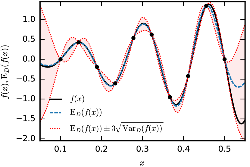
Figure 1: The 1-dimensional emulator as constructed in §3.2. The dashed (blue) line is the emulator prediction ${\rm E}_{D}(f(x))$ as a function of $x$, and the credible interval ${\rm E}_{D}(f(x))\pm 3\sqrt{{\rm Var}_{D}(f(x))}$ is given by the dotted (red) lines. The true function $f(x)$ is shown as the black solid line, and the 10 model runs that make up the vector $D$ used to build the emulator are given as the red points.

Fig. 1 shows the 1-dimensional emulator where ${\rm E}_{D}(f(x))$ as a function of $x$ is given by the dashed blue line, and the credible interval ${\rm E}_{D}(f(x))\pm 3\sqrt{{\rm Var}_{D}(f(x))}$ by the dotted red lines. We can see that ${\rm E}_{D}(f(x))$ precisely interpolates the known runs at outputs $D$, with zero uncertainty (as the red lines touch at these points): a desirable feature as here $f(x)$ is a deterministic function. The credible regions get wider the further we are from known runs, appropriately reflecting our lack of knowledge in these regions. The true function $f(x)$ is given by the solid black line which lies within the credible region for all $x$, only getting close to the boundary for $x>0.5$. This demonstrates the power of an emulator: using only a small number of runs we can successfully mimic relatively complex functions to a known accuracy, a feature that scales well in higher dimensions due to the chosen form of the emulator. The speed of Bayesian emulators is also crucial for global parameter searches where we may need to evaluate the emulator a huge number of times to fully explore the input space. Note that the emulator calculation is extremely fast because it only requires matrix multiplication for each new $x$. The inverse ${\rm Var}(D_{i})^{-1}$ that features in equations (3.1) and (3.1) is independent of $x$ (and indeed of $D_{i}$) and hence can be performed only once, offline and in advance of even the run evaluations $D_{i}$.

3.3 Emulating in Higher Dimensions

When emulating functions possessing high input dimension, the polynomial regression terms $\beta_{ij}g_{ij}(x_{A_{i}})$ in the emulator equation (15) become more important, as they efficiently capture many of the more global features often present in the physical model (Vernon et al., 2010a, b). Prior specifications for the $\beta_{ij}$ can be given, based say on structural knowledge of the model, or on past experience running a faster but simpler previous version of the model (Cumming & Goldstein, 2009a). However, if no strong prior knowledge is available and the number of runs performed is reasonably high, a vague prior limit can be taken in the Bayes Linear update equations (3.1) and (3.1), resulting in the adjusted expectation and variance of the $\beta_{ij}$ terms tending toward their Generalised Least Squares (GLS) estimates. For space filling runs, such as those from a maximin latin hypercube, the GLS estimates can be accurately approximated by the corresponding Ordinary Least Squares (OLS) estimates, which can also be used to estimate $\sigma_{u_{i}}^{2}$, providing further efficiency gains (Vernon et al., 2010a).

In addition, the choice of active input variables $x_{A_{i}}$ and the choice of the specific regression terms $\beta_{ij}g_{ij}(x_{A_{i}})$ that feature in the emulator, can both be made using linear model selection techniques based on AIC or BIC criteria. For example, these can be simply employed using the lm() and step() functions in R (Vernon et al., 2010a; R, 2015). The use of active variables $x_{A_{i}}$ can lead to substantial dimensional reduction of the input space of each of the outputs, and hence convert a high dimensional problem into a collection of low dimensional problems, which is often far easier to analyse (see Vernon et al., 2010b, for further discussion of this benefit). It is worth noting that reasonably accurate emulators can often be constructed just using such regression models. This can be a sensible first step (see Andrianakis et al., 2016b), before one attempts the construction of a full emulator of the form given in equation (15).

3.4 Iterative History Matching via Implausibility

We now describe the powerful iterative global search method known as History Matching (Craig et al., 1996, 1997), which naturally incorporates the use of Bayesian emulators, and which has been successfully applied across a variety of scientific disciplines. It aims to identify the set $\mathcal{W}$ of all inputs $x$ that would give rise to an acceptable match between the galform outputs $f(x)$ and the corresponding vector of observed data $w$, and proceeds iteratively, discarding regions of input space which are deemed implausible based on information from the emulators. For more detail on the contents of this section see (Vernon et al., 2010a, b).

For an output $f_{i}(x)$ we define the implausibility measure:

$$I_{i}^{2}(x,w_{i})\;\;=\;\;\frac{({\rm E}_{D_{i}}(f_{i}(x))-w_{i})^{2}}{{\rm Var}_{D_{i}}(f_{i}(x))+\sigma^{2}_{\epsilon_{i}}+\sigma^{2}_{e_{i}}}$$ (27)

which takes the distance between the emulator’s prediction of the $i$th output ${\rm E}_{D_{i}}(f_{i}(x))$ and the actual observed data $w_{i}$ and standardises it with respect to the variances of the three major uncertainties: the emulator uncertainty ${\rm Var}_{D_{i}}(f_{i}(x))$, the model discrepancy $\sigma^{2}_{\epsilon_{i}}$ and the observation error $\sigma^{2}_{e_{i}}$.

The least familiar of these is the model discrepancy $\sigma^{2}_{\epsilon_{i}}$ which is an upfront acknowledgement of the deficiencies of the galform model in terms of assumptions used, missing physics and simplifying approximations. In addition to ensuring the analysis is more meaningful, this term guards against overfitting, and the subsequent technical and robustness problems this can cause for a global parameter search. See Kennedy & O’Hagan (2001); Brynjarsdottir & O’Hagan (2014); Goldstein & Rougier (2009) for extended discussions on this point. The form of the implausibility comes from the “best input approach” which models the link between the galform model evaluated at its best possible input $x^{*}$ and the real Universe $y$ as $y=f(x^{*})+\epsilon$, where $\epsilon$ is a random quantity representing the model discrepancy with variance $\sigma^{2}_{\epsilon}$, and assumes that the observed data $w$ is measured with uncertain error $e$ with variance $\sigma^{2}_{e}$, such that $w=y+e$. See Craig et al. (1997); Vernon et al. (2010a, b) for further justifications and discussions.

Most importantly, a large value of the implausibility $I_{i}(x,w_{i})$ for any output implies that the point $x$ is unlikely to yield an acceptable match between $f(x)$ and $w$ were we to run the galform model there, hence $x$ is deemed implausible and can be discarded from further analysis. We therefore impose cutoffs of the form $I_{i}(x,w_{i})<c$ to rule out regions of input space, where the choice of $c$ is motivated from Pukelsheim’s 3-sigma rule (Pukelsheim, 1994). We can combine the implausibility measures from several outputs in various ways e.g.

$$I_{M}(x,w)\;\;=\;\;\max_{i\in Q}I_{i}(x,w_{i})$$ (28)

where $Q$ represents the subset of outputs currently considered (often we will only emulate a small subset of outputs in early iterations). We may use the second or third maximum implausibility instead for robustness reasons, or use multivariate implausibility measures to incorporate correlations (Vernon et al., 2010a, b).

History matching proceeds iteratively, discarding implausible regions of the input parameter space in waves. At the $k$th wave we define the current set of non-implausible input points as $\mathcal{W}_{k}$ and the set of outputs that have so far been considered for emulation as $Q_{k}$. We proceed according to the following algorithm:

• 1. Design and evaluate a space filling set of wave $k$ runs over the current non-implausible space $\mathcal{W}_{k}$.

  2. Check if there are informative outputs that can now be emulated accurately (that were difficult to emulate in previous waves) and add them to $Q_{k}$, to define $Q_{k+1}$.

  3. Use the wave $k$ runs to construct new, more accurate emulators defined only over the region $\mathcal{W}_{k}$ for each output in $Q_{k+1}$.

  4. Recalculate the implausibility measures $I_{i}(x,w_{i})$, $i\in Q_{k+1}$, over $\mathcal{W}_{k}$, using the new emulators.

  5. Impose cutoffs $I_{i}(x,w_{i})<c$ to define a new, smaller non-implausible volume $\mathcal{W}_{k+1}$ which satisfies $\mathcal{W}\subset\mathcal{W}_{k+1}\subset\mathcal{W}_{k}$.

  6. Unless:

     1. the emulator variances ${\rm Var}_{D_{i}}(f_{i}(x))$ are now small in comparison to the other sources of uncertainty: $\sigma^{2}_{\epsilon_{i}}+\sigma^{2}_{e_{i}}$,

     2. the entire input space has been deemed implausible or

     3. computational resources have been exhausted,

     return to step 1.

  7. If 6A is true, generate a large number of acceptable runs from the final non-implausible volume $\mathcal{W}$, using appropriate sampling for the scientific purpose.

We are then free to analyse the structure of the non-implausible volume $\mathcal{W}$ and the behaviour of model evaluations from different locations within it. The history matching approach is powerful for several reasons:

• As we progress through the waves and reduce the non-implausible volume, we expect the function $f(x)$ to become smoother, and hence to be more accurately approximated by the regression part of the emulator $\beta_{ij}g_{ij}(x_{A_{i}})$ (which is often composed of low order polynomials – see equation 15).

• At each new wave we have a higher density of points in a smaller volume, therefore the emulator’s Gaussian process term $u_{i}(x_{A_{i}})$ will be more effective, as it depends mainly on the proximity of $x$ to the nearest runs.

• In later waves the previously strongly dominant active inputs $x_{A_{i}}$ from early waves will have had their effects curtailed, and hence it will be easier to select additional active inputs, unnoticed before.

• There may be several outputs that are difficult to emulate in early waves (often due to their erratic behaviour in scientifically uninteresting parts of the input space) but simple to emulate in later waves, once we have restricted the input space to a much smaller and more physically realistic region.

History matching can be viewed as the appropriate analysis suitable for model investigation, model checking and model development. Should one wish to perform a fully Bayesian analysis using say MCMC, history matching can be used as a highly effective precursor to such a calculation in order to rule out vast regions of input space that would only contain extremely low posterior probability. However such an MCMC analysis would only be warranted assuming one is willing to specify meaningful joint probability distributions over all uncertain quantities involved, in contrast to only the expectations, variances and covariances required for the Bayes Linear history match.

3.5 Application of Emulation and History Matching to galform and the GSMF

We now apply the above Bayesian emulation and history matching methodology to galform and the GSMF, and generalise it to the case of multiple available observed data sets. We first identify the galform model outputs $f_{i}(x)$ that we wish to emulate, and the corresponding observed data $w_{i}^{(m)}$ to match them to as

$$f_{i}(x)=\log\phi_{i,\text{model}}\quad\text{and}\quad w_{i}^{(m)}=\log\phi_{i,\text{obs}_{(m)}}$$ (29)

where

$$\phi_{i}=\left.\frac{\operatorname*{d\!}n}{\operatorname*{d\!}\log M_{\star}}\right|_{M_{\star,i},z}$$

is the GSMF at the stellar mass bin $M_{\star,i}$ for redshift $z$. Here $m$ labels the choice of observed data sets we use, represented for output $i$ by $w_{i}^{(m)}$. Following the discussion in Bower et al. (2010), we adopt a model discrepancy of 0.1 dex. This term summarises the accuracy we expect for the model due to the approximations inherent in the semi-analytic method. In effect, this means that we will regard models that lie within 5% of the observed data-point as a perfectly adequate fit, even if the quoted Poisson observational errors are substantially smaller. This means that if a model has a marginally acceptable implausibility, $\,I\sim 3$, it may be 0.3 dex away from the observational data-point.

As we have multiple sets of observed data for the GSMF which we wish to match to, we have to make an additional decision as to how to combine these within the history matching process. Here we generalise the implausibility measure of equation (28) by minimizing over the $m$ data sets:

$$I_{M}(x,w)\;\;=\;\;\max_{i\in Q}\{\min_{m}I_{i}(x,w_{i}^{(m)})\}$$ (30)

with the second and third maximum implausibilities defined similarly. This implies that our history match search will attempt to find all inputs that lead to matches to any of the observed data sets, judged on an individual bin basis. This is a simple way of incorporating several (possibly conflicting) data sets into the history match that does not involve additional assumptions or further statistical modelling, and which is sufficient for our current purposes. It should lead to the identification of all inputs of interest, subsets of which (for example those that match a specific data set, or a combined data set) can be subsequently explored in further detail.

The emulators used in each wave were constructed following the techniques described in §3.1, §3.2 and specifically the high dimensional approaches of §3.3.

3.6 Observational datasets used

For the local Universe GSMF, we use the results of Li & White (2009) based on SDSS and Baldry et al. (2012) on the GAMA survey.

For larger redshifts, we combine the results of Tomczak et al. (2014) based on the zfourge and candels surveys, and Muzzin et al. (2013), based on the UltraVISTA survey. In these papers, the GSMF is reported for redshift intervals/bins. For simplicity, we adopt the midpoint of each redshift bin as the typical redshift to be compared with the model (e.g. the GSMF obtained for $0.5<z<1.0$ will be compared with the model results for $z=0.75$). Both datasets obtain their stellar masses using the fast code (Kriek et al., 2009) to fit the stellar population synthesis model of Bruzual & Charlot (2003) to the measured spectral energy distributions of the galaxies, assuming a Chabrier (2003) IMF. Errors in the determination of galaxy masses at $z>0$ redshifts were assumed to follow the redshift-dependent estimate as Behroozi et al. (2013), i.e. $\sigma_{M}(z)=\sigma_{0}+\sigma_{z}z$, with $\sigma_{0}=0.07$ and $\sigma_{z}=0.04$. These mass errors were accounted for convolving the model GSMF with a Gaussian kernel (see §4.2 for a discussion).

Table 2: Thresholds used for eliminating implausible regions with respect to the local Universe GSMF after each wave and the fraction of the initial volume in the non-implausible region.

Wave	Threshold			Fraction of the
	1st max.	2nd    max.	3rd    max.	initial volume
1	-	3.2	2.5	0.2522
2	4.5	3.0	2.3	0.0494
3	3.75	2.5	2.0	0.0170
4	3.5	2.5	2.0	0.0116
5	3.0	2.25	2.0	0.0036
6	2.4	2.15	1.8	0.0010

4 Results

The parameter space exploration was conducted through successive waves of runs. After each wave, emulators were generated from its results and used to design the parameter choices for the next wave, discarding a vast, specifically implausible, region of the parameter space. Each wave was designed using a Latin Hypercube Sampling of $5000$ points of the non-implausible region of the parameter space (full details are given in appendix A).

4.1 Matching the local galaxy stellar mass function

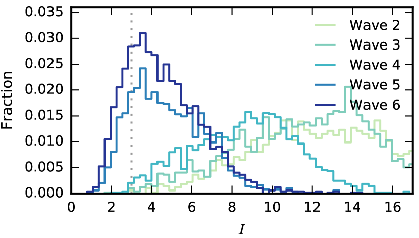
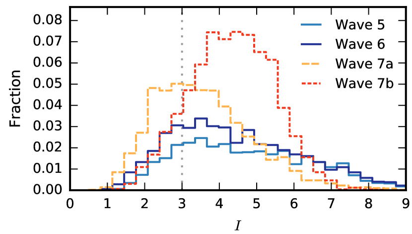
Figure 2: Histograms of the model implausibilities (with respect to the local Universe only) obtained at each wave. In the top panel, exploratory waves 2-6 are shown. Each new wave reduces the tail of very implausible models. However, the increase in the number of models with $I<2$ occurs only slowly after each wave. In the bottom panel, waves 7a and 7b are also shown (please, note the different range in $I$). Wave 7a was designed specifically to obtain many plausible runs, instead of uniformly covering the non-implausible parameter space, and Wave 7b (discussed in §4.2) takes into account the constraints by high redshift data.

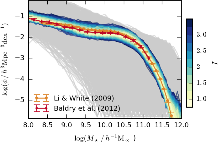
Figure 3: Local galaxy stellar mass function. The coloured curves show all the runs with implausibility $I<3.5$, with different shades showing different implausibilities (see colour-bar in the plot). The surrounding light grey curves correspond to the initial set of runs (wave 1). Data-points show the GSMF data obtained by Li & White (2009) and Baldry et al. (2012). Note that a 0.1 dex model discrepancy was assumed (see text for details).

There were initially 6 waves of runs, where the implausibilities were computed with respect to the local Universe GSMF data only. Table 2 shows the implausibility cut-off thresholds applied, which decreased after each wave as we build more trustworthy emulators. Table 2 also shows the fraction of the initial volume which corresponds to the region classified as non-implausible after each wave. To compute the volumes, the parameters were rescaled following equations (1) and (2) – i.e. lengths associated with the range of each parameter were considered equivalent. Despite making very conservative choices for the thresholds, there is a strong decrease in the volume after each wave and after wave 6 only $10^{-3}$ of the original volume was classified as non-implausible. In Fig. 2 the evolution of the distribution of the implausibilities can be followed: after each wave the number of highly discrepant models is strongly reduced, but the number of acceptable models, with $I<3$, increases only modestly.

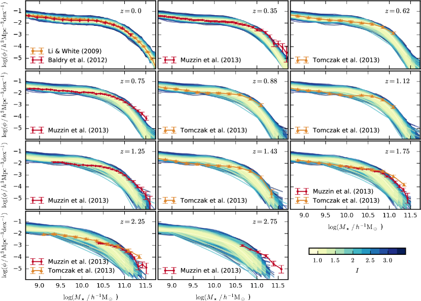
Figure 4: The GSMF of selected models colour-coded by their implausibility, $I$ (see colour bar), calculated only with respect to the GSMF data at the local Universe, from Baldry et al. (2012) and Li & White (2009). Only runs with $I<3.5$ with are shown. The high redshift observational data shown were obtained from Muzzin et al. (2013) and Tomczak et al. (2014). The models selected solely by their good match to $z=0$ data produce poor agreement to higher redshift data.

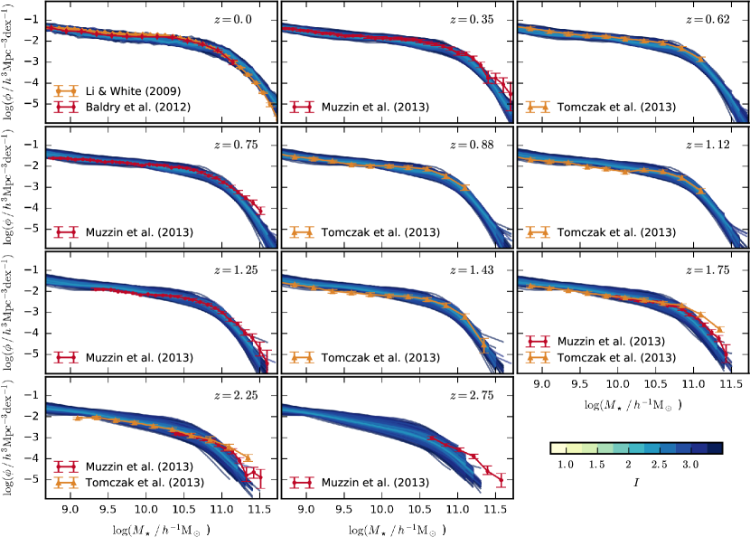
Figure 5: The GSMF of selected models colour-coded by their implausibility, $I$, calculated simultaneously with respect to the GSMF at $z=0,\,0.35,\,0.62,\,0.75,\,0.88,\,1.12,\,1.25$ and $1.43$. Only runs with $I<3.5$ are shown. The high redshift observational data shown were obtained from Muzzin et al. (2013) and Tomczak et al. (2014) and local Universe data were obtained from Baldry et al. (2012) and Li & White (2009). galform models generally lead to a GSMF with a high mass end which is too shallow at $z=0$ and too steep at higher redshifts.

After the 6^th wave the emulator variance at each point was already smaller or equal to the other uncertainties, indicating that no further refinement was possible (condition 6A in the algorithm described in §3.4). A final, wave 7a, was then designed, this time using the emulator information to aim for the best possible matches to the GSMF (i.e. step 7 in the algorithm; in contrast to the previous waves where the non-implausible space was uniformly sampled to ensure an optimum input for the next wave).

In Fig. 3, the final results of the history matching are shown, together with our observational constraints. Error bars in this and other figures show only the quoted observational errors, and do not include the model discrepancy term, so that the over all quality of the fits can be judged from figures. The purpose of the model discrepancy is to avoid rejecting models when the observational errors become very small. All the models in our library with implausibility $I<3.5$ are shown in Fig. 3, with the curves colour-coded by the implausibility. The width of the lightest shade, corresponding to $I\leq 1.0$, allows one to visualize the effect of adopted model discrepancy. Also shown are the wave 1 runs given as the grey curves, many of which were far from the observed data. The impact of the history match in terms of the removal of substantial amounts of implausible regions of the parameter space can be seen by comparing the coloured region with the grey curves.

While there are models with $I\sim 2.5-3$ which produce an excess in the number of small mass galaxies, the opposite (i.e. $\phi$ smaller than the observations at the low mass end) is very rare. A similar behaviour is also present in the high mass end. Thus, acceptable ($I\lesssim 3$) models may display over-abundances of very small [$\log(M_{\star}/\,\text{M}_{\odot})\lesssim 8.5$] or very large [$\log(M_{\star}/\,\text{M}_{\odot})\gtrsim 11.5$] masses, but there are no acceptable models with significant under-abundances in these ranges.

Once the locus of models with good fits to the local Universe GSMF was found, we examined how well these models performed with respect to high redshift data. In Fig. 4 the GSMF output by the models shown in Fig. 3 is now compared with higher redshift data. One finds that the models selected only by their ability to reproduce the local Universe GSMF data under-represent the abundance of high mass galaxies at higher redshifts while simultaneously generating an excessive number of galaxies of lower masses.

In the following section we will examine the parameter space and show that the vast majority of acceptable models have $\beta_{0,\text{burst}}>\beta_{0,\text{disc}}$ and so lie in a region of parameter space not available to the original model.

4.2 Constraining models with higher redshift data

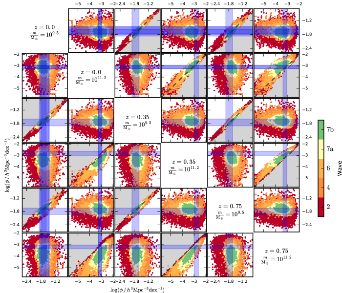
Figure 6: Each panel compares the output of the GSMF for different mass bins and/or redshifts. Waves 2, 4, 6, 7a, 7b are shown colour-coded as indicated. The observational constraints of previous figures are shown as blue shades. The light grey shade was added to guide the eye, indicating where the GSMF values in the vertical axis are smaller than the horizontal axis, and the dashed diagonal line indicates the case where the GSMF for the two is the same. Panels below the diagonal use the same estimates for the errors in the mass determination as Behroozi et al. (2013): $\sigma_{M}=0.07+0.04\,z$ (see text for details). For comparison, in the panels above the diagonal we double the mass error. After successive waves there is improvement in the agreement with the low redshift data and with the low-mass-end of the high redshift data, however, for the high-mass end, there is still tension at higher redshifts. The increase in the mass error does not avoid the tension. This tension originates from the data being consistent with small or no evolution for bins of large mass.

To investigate if, and to what extent, the present model could reproduce the evolution of the GSMF, a new wave of runs was generated from the wave 6 emulator (wave 7b), this time computing the implausibilities simultaneously with respect to the GSMF data at higher redshifts, up to $z=1.75$.

After just a single additional wave, the emulation technique indicated that no extra refinement was likely: the emulator variances became smaller than the other uncertainties, corresponding to step 6A in the algorithm of §3, suggesting that it would be highly unlikely to find a locus of more plausible runs within any sub-volume of the parameter space. A new (and final) wave was then designed, to produce runs which provided a good match to the GSMF at those redshifts (corresponding to step 7). This set of runs was deliberately focused towards the regions of lowest emulator implausibility, where we would now expect the best matches to occur. This is a good technique for exploring the correlations between parameter sets; however, it is important to note that the resulting design of runs would not be a suitable basis for the construction of a statistical emulator.

In Fig. 5 we show the evolution of the GSMF for all the runs (of all waves) with implausibility $I<3.5$ with respect to redshifts up to $z=1.12$. The adoption of higher redshift constraints leads to tension with the local Universe data: the least implausible models produce a GSMF with a too shallow high mass end at $z=0$ and too steep at any other redshift. In the low mass end, there is an excess of $\lesssim 10^{10}\,\text{M}_{\odot}$ galaxies at higher redshift and a small deficit of them in the local Universe. This is consistent with behaviour seen in the runs constrained at $z=0$ only. It should be noted that, despite the tension, the level agreement achieved is still better than what is found in most published models, and is not dissimilar from what is found by Henriques et al. (2013); Henriques et al. (2015).

This tension becomes clearer when the results for specific mass bins of the GSMF are compared. This is shown in panels below the diagonal in Fig. 6, for two mass bins, $\log(m/\,\text{M}_{\odot}h)=9.5$ and $11.2$, redshifts $z=0.0$, $0.35$ and $0.75$. The observational constraints are shown as blue bands. By showing the constraints in pairs, we gain insight into the conflicting pressures imposed on the model. Initially, successive waves of runs (shown by colours from red to green, as indicated in the figure) are increasingly focused towards the point at which the two bands intersect. However, it becomes increasingly evident that some constraint pairs cannot be matched by the model and the successive waves lead to no improvement. For example, the panel showing $\log(m/\,\text{M}_{\odot}h)=11.2$ at $z=0$ and $z=0.35$ has a strong diagonal line above which the model is never able to cross. The same behaviour is found when comparing the high mass end of the GSMF at $z=0$ with other redshifts. For the constraints at $\log(m/\,\text{M}_{\odot}h)=9.5$, the outputs of all models are tightly correlated when comparing between redshift. Comparison between different mass bins appears to be less constraining.

One can best interpret Fig. 6 by comparing the models to a non-evolving GSMF. This is shown by the dashed diagonal line in panels that compare the same mass bins. The grey-shaded side of the dashed diagonal line show the case where the number of galaxies decreases with time. It can be seen that the observational data used leads to no evolution (or even decrease) in the number of $10^{11.2}h^{-1}\,\text{M}_{\odot}$ galaxies if $z=0$ is compared to other datasets. This makes it clear why it is not possible to find models in the exact target region. Since galform is inherently hierarchical, it is difficult to conceive of a mechanism which could lead to a significant decrease in the abundance of massive galaxies with time. This would only be possible if $10^{11.2}h^{-1}\,\text{M}_{\odot}$ galaxies were to grow in mass (and so leave the mass bin) faster than lower mass (and more abundant) galaxies were able to grow and move into the bin. Clearly, the situation never arises in the galform model and the only way of obtaining points in the grey region for the high mass bin panes is due to the distortion caused by errors in the galaxy mass determination, as we will discuss below.

Systematic errors in the determination of galaxy masses (‘mass errors’ for short) arising from the modelling of the star formation history, choice of dust model and the choice of IMF can significantly affect the shape of the GSMF which is inferred from the observations (Mitchell et al., 2013). As mentioned in §3.6, mass errors were accounted for by convolving the model GSMF with a Gaussian kernel. The main effect of such convolution is making the GSMF appear less steep at higher redshifts. This raises the question of whether underestimated mass errors could explain the difficulty in simultaneously matching the high mass end of the GSMF at different redshifts.

In the panels above the diagonal of Fig. 6, we show the consequences of doubling the mass error – i.e. considering $\sigma_{0}=0.14$ and $\sigma_{z}=0.08$. This has the effect of loosening the implausibility contours: the blue regions are the same as those below the diagonal. The effect of these much increased mass errors is to allow models near to the “no evolution” region, alleviating the tension by allowing the corrected galform results to get closer to the target region. However, even considering these mass errors, some tension still persists.

4.3 Plausible models subspace

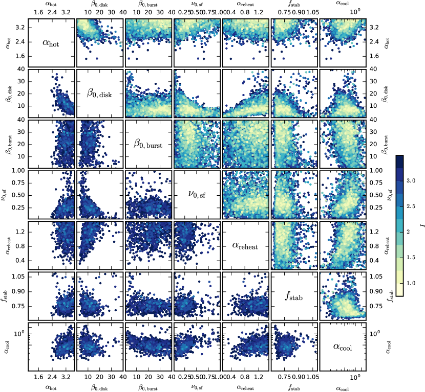
Figure 7: The panels show two dimensional projections of the plausible parameter space. Each circle represents a galform run and is colour coded by its implausibility (as indicated by the colour bar); lower implausibility runs are plotted on top facilitating the visualisation of their clustering in the projected space; only runs with $I<3.5$ are shown. In panels above the diagonal, the implausibility is computed with respect to the observed local GSMF only. In panels below the diagonal, the implausibility is computed with respect to the GSMF at redshifts $z=0.0,\,0.35,\,0.62,\,0.75,\,0.88,\,1.12,\,1.25$ and $1.43$. Note that the axes are labelled consistently above and below the diagonal. A panel below the diagonal should be rotated and inverted in order to compare it to the equivalent panel above the diagonal. This figure summarizes the main constraints imposed by the GSMF and its evolution on the galform parameters.

We examine now what are the main properties of the subspace of plausible models, which we define as models having implausibility, $I<3.5$, a conservative threshold.

We begin by considering the models that provide a plausible match to the GSMF at $z=0$. The distribution of these models are shown above the diagonal in Fig. 7. In each panel we show the plausible models projected into the two dimensional space of a pair of variables. The models are coloured by implausibility and the lowest implausibility runs are plotted last to ensure they are visible. This method of plotting also gives a good impression of the “optical depth” of the parameter region in the hidden parameters of each panel. We only show the most interesting variables in this plot, the panels for other variable pairs are less informative scatter plots.

The most constrained parameters are: the disk wind parameters, $\alpha_{\text{hot}}$ and $\beta_{0,\text{disc}}$, the normalisation of the star formation law, $\nu_{0,\text{sf}}$, the AGN feedback parameters, $\alpha_{\text{cool}}$, and the disk stability threshold, $f_{\rm stab}$. Several parameter degeneracies can be picked out in the figure. For example, values of $\alpha_{\text{hot}}$ are strongly correlated with $\beta_{0,\text{disc}}$, with larger $\beta_{0,\text{disc}}$ being compensated by a smaller $\alpha_{\text{hot}}$: i.e., the higher mass loading normalisation is compensated by a weaker mass dependence so that the level of feedback is similar in low-mass galaxies.

Other parameters are more weakly constrained, and it is possible to find plausible models over most of the range of the parameter considered. The parameter $\alpha_{\text{reheat}}$ is a good example. In this case, smaller values of $\alpha_{\text{reheat}}$ can be compensated by reductions in $\beta_{0,\text{disc}}$. This makes physical sense. The time-scale on which gas is re-incorporated into the halo after ejection depends on $\alpha_{\text{reheat}}^{-1}$ (equation 11), so that increases in the time-scale can be offset by an overall lower mass loading of the disk wind (Mitchell et al., 2016).

One surprising feature is that the normalization mass loading associated with star burst galaxies, $\beta_{0,\text{burst}}$, (see §2.2.3) is weakly constrained. Although the best models (and also the greatest number of models) have $\beta_{0,\text{burst}}>20$, entirely plausible models can be found with much smaller values. This is presumably because the impact of the large values of $\beta_{0,\text{burst}}$ can be offset by adjusting the values of other parameters. The pairs plot does not, however, reveal an obvious interaction with another individual parameter. In §4.4, we will use a principle component method to try to isolate simpler interactions between parameter combinations, and we explore the physical interpretation there.

The panels below the diagonal line show the models that generate plausible fits to the GSMF over the redshift range $z=0$ to $1.43$. A panel below the diagonal must be rotated and inverted in order to compare it to the equivalent panel above the diagonal. As we have already discussed, this is a stringent requirement, and even the best models have $I>2$. The volume of the parameter space within which plausible models can be found is significantly reduced compared to the situation if only the $z=0$ implausibility is considered. The plausible range of the parameters $\alpha_{\text{reheat}}$, $\alpha_{\text{cool}}$ and $\nu_{0,\text{sf}}$ is particularly affected. For example, the addition of the high redshift GSMF excludes very long gas cycling time-scales (and thus small values of $\alpha_{\text{reheat}}$).

Plotting the data in this way does not, however, expose any new correlations between parameters, or make it easy to appreciate the physical differences in the model that result in the very different behaviour at high redshift that can be seen by comparing Figs. 4 and 5. In order to make it easier to identify these differences, we will analyse the distribution of the plausible models in the Principle Component Analysis (PCA) space. This allows us to better identify the critical parameter combinations that are picked out by the data. We have already noted that several parameters show significant (anti-)correlation, and the PCA analysis will identify the most important relations.

One of the motivations for undertaking a full parameter space exploration is the possibility of the existence of multiple disconnected implausibility minima, which would be unlikely to be found in the ‘traditional’ trial-and-error approach to choosing the parameters. Nevertheless, we find that the locus of acceptable galform runs is connected and there are no signs of multiple minima or other complex shapes. Because of this, the distribution of plausible models is particularly amenable to the PCA method.

4.4 Principal component analysis

In order to obtain greater insight into the constraints imposed by the GSMF, and in particular the constraints imposed by the higher redshift data, we performed a principal component analysis (PCA) on the volume of the input parameter space containing runs with $I<3.4$ in all the datasets at $z=0,\,0.35,\,0.62,\,0.75,\,0.88,\,1.12,\,1.25$ and $1.43$, giving a set of 508 runs in total. The PCA generates a new set of 20 orthogonal variables defined as the eigenvectors of the covariance matrix formed from the input parameter locations of the 508 runs, ordered by size of eigenvalue. Therefore the first new variable (Var 1) gives the direction which has the largest variance in the input space, while the last (Var 20) gives the direction with the smallest variance. Usually, PCA is applied to find the directions with the largest variance, but here we are precisely interested in the opposite: we wish to learn about those directions in input parameter space that have been most constrained by the observed data. This analysis allows the examination of the location of acceptable runs in the rotated (and translated) PCA space, to identify possible hidden features, and the transformation of the (approximately) orthogonal constraints observed in the PCA space back on to the original parameters to aid physical interpretation. For example, acceptable model runs all have similar values for Var 20, Var 19 etc, and this can be inverted to express the dependencies of the variables on one another. It is important to note that the precise components of the PCA variables depend on their original range (and whether the variables are normalised on to a log or linear scale). This can be viewed in a Bayesian sense, in that we are quantifying the increase in knowledge about the values of the variables relative to our prior knowledge. It is also important to bear in mind that variables with similar variance are degenerate, and that alternative combinations of them will describe the distribution of the data similarly well, but may have a simpler physical interpretation.

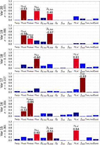
Figure 8: Summary of results of the principal component analysis. The 6 most constrained components of the region with $I<3.4$ with respect to $z=0,\,0.35,\,0.62,\,0.75,\,0.88,\,1.12,\,1.25$ and $1.43$ (which contains 508 models). The bars show the absolute values of the PCA loads associated with each scaled parameter (only parameters with non-negligible loads are shown). Parameters with larger loads ($>0.3$) are drawn in red and have their names and loads written on the top of the bars. Bright (dark) colours show variables with positive (negative) loads.

The resulting PCA variables (and the centroid of the distribution) are listed in Appendix B. The standard deviation in the directions defined by Var 20 and Var 19 is extremely small (less than 0.1 relative to the prior distribution of $\pm 1$). Var 18 and Var 17 are also significantly constrained (std. dev. less than 0.22). The constraints on the other variables are much less significant, Var 14, 15 and 16 all have std. dev. $\sim 0.4$. This gives us a quantitative measure of the information content of the GSMF relative to the freedoms of the model.

The components of the 6 most constrained variables are shown in Fig. 8. We begin by considering the strongly constrained components Var 19 and Var 20. The variance of these two components is similar and so we should consider them together. As shown by the colouring of the histogram, Var 19 is dominated by $\beta_{0,\text{disc}}$ and $\alpha_{\text{cool}}$, with a smaller contribution from $\alpha_{\text{reheat}}$. Qualitatively, this simply confirms that the break of the GSMF is controlled by competition between AGN and stellar feedback; stronger winds from disks in $200\,\text{km}\,\text{s}^{-1}$ galaxies (i.e., larger $\beta_{0,\text{disc}}$, equation 9), or a longer re-incorporation time-scale (i.e., smaller $\alpha_{\text{reheat}}$, equation 11), need to be compensated by an increase the halo mass at which AGN become effective (i.e., smaller $\alpha_{\text{cool}}$, since $t_{\text{cool}}/t_{\text{ff}}(r_{\text{cool}})$ increases with halo mass, equation 12). As well as providing qualitative insight, this can be translated into quantitative constraints on the input parameters. To do this we neglect the dependence on parameters with small loads ($<0.3$, shown in blue in Fig. 8) and assume that they have values close to the centroid of the PCA expansion. Using superscripts to denote that this relation applies to the rescaled variables (given by equations 1 and 2), the constraint can then be simplified to:

$$|\text{Var}\,19|\,= \,\,|\,-0.669(\beta_{0,\text{disc}}^{(s)}+0.464)-0.576(\alpha_{\text{cool}}^{(l)}-0.065)$$

$$+0.356(\alpha_{\text{reheat}}^{(s)}-0.462)\,|\,\,\lesssim 0.095.$$ (31)

Var 20 is mainly composed of $\alpha_{\text{cool}}$ (the AGN feedback parameter), $\alpha_{\text{hot}}$ and $\beta_{0,\text{disc}}$ (the quiescent feedback parameters). Eliminating variables with small weight, we arrive at the following inequality:

$$|\text{Var}\,20|\,= \,\,|\,+0.401(\beta_{0,\text{disc}}^{(s)}+0.464)+0.583(\alpha_{\text{hot}}^{(s)}-0.673)$$

$$-0.634(\alpha_{\text{cool}}^{(l)}-0.065)\,|\,\,\lesssim\,0.071.$$ (32)

Physicaly, this relation tells us that if we pick the disk feedback parameters $\alpha_{\text{hot}}$ and $\beta_{0,\text{disc}}$, the AGN feedback must follow from the equality. Increases in $\alpha_{\text{hot}}$ and/or $\beta_{0,\text{disc}}$ (making supernovae driven feedback) need to be compensated by increases $\alpha_{\text{cool}}$ (making AGN feedback effective only in higher mass haloes). Since Var 19 already determines $\alpha_{\text{cool}}$, it is more useful to write the constraint as (neglecting small weights):

$$|\text{Var}\,20|\,\approx \,\,|\,+1.137(\beta_{0,\text{disc}}^{(s)}+0.464)-0.391(\alpha_{\text{reheat}}^{(s)}-0.462)$$

$$+0.583(\alpha_{\text{hot}}^{(s)}-0.673)\,|\,\,\lesssim\,0.175,$$ (33)

which expresses the requirement that a given choice of $\beta_{0,\text{disc}}$ (and $\alpha_{\text{reheat}}$) parameters need to be balanced by a suitable choice of circular velocity dependence of supernova feedback, $\alpha_{\text{hot}}$.

The next two components, Var 18 and Var 17, have significantly larger variances ($\sigma=0.174$ and $0.217$, respectively). Var 17 is almost completely determined by $f_{\rm stab}$, so that successful models require a narrow range of the stability parameter, almost independent of the other variables.

$$|\text{Var}\,17|\,=\,\,|\,-0.931(f_{\rm stab}^{(s)}+0.362)\,\,\,|\,\,\lesssim 0.217\,.$$ (34)

Var 18 relates the star formation efficiency $\nu_{0,\text{sf}}$ to $\alpha_{\text{hot}}$, the halo mass dependence of feedback (which in turn relates to the choice of feedback parameters $\beta_{0,\text{disc}}$ and $\alpha_{\text{reheat}}$, see equation 33):

$$|\text{Var}\,18|\, =\,\,|\,\,0.613(\nu_{0,\text{sf}}^{(s)}+0.456)$$

$$-0.604(\alpha_{\text{hot}}^{(s)}-0.673)\,\,\,|\,\,\lesssim 0.174.$$ (35)

Increasing the strength of feedback in small galaxies (greater $\alpha_{\text{hot}}$) requires that star formation is made more efficient to compensate (i.e. by increasing star formation at higher mass galaxies, maintaining thus the total amount of stars at low $z$).

The remaining variables are relatively weakly constrained, but have similar variance. They provide addition constraints on the disk and AGN feedback parameters ($\alpha_{\text{reheat}}$, $\alpha_{\text{cool}}$, $\alpha_{\text{hot}}$ and $\beta_{0,\text{disc}}$) and the star formation law ($\nu_{0,\text{sf}}$). Although they are weakly constrained, these relations play an important role in determining whether models successfully match the higher redshift GSMF data as well as the $z=0$ GSMF, as we will show below.

4.5 Effect of GSMF constraints in PCA space

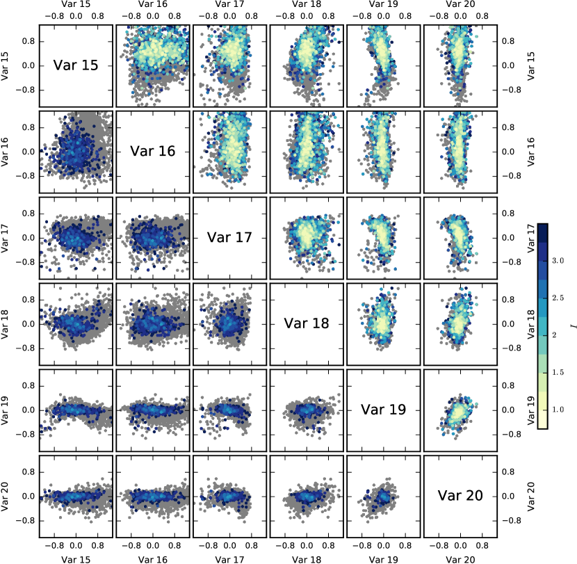
Figure 9: A comparison of runs that provide plausible fits to the $z<1.43$ GSMF datasets (below the diagonal), and those that provide a plausible description of the $z=0$ GSMF, but a very implausible match to the high-z data (above the diagonal). We show the comparison PCA-space, with individual panels showing two dimensional projections. The PCA variables are defined using the set of plausible $z<1.43$ GSMF datasets. We show the 6 most constrained variables (see text for discussion). Each circle represents a galform run and is colour coded by its implausibility (as indicated by the colour bar); lower implausibility runs are plotted on top to facilitate the visualisation of their clustering in the projected spaced. To facilitate comparison of the runs above and below the diagonal, we show the full set of runs with plausibly fits to the $z=0$ GSMF as the underlying grey points.

In order to better understand why some runs generate a plausible match to the $z<1.43$ GSMF (as well as that at $z=0$) while others do not, we select the 5 components with least variance and rotate the distribution of the full set of runs with plausible $z=0$ into this space. Note that the variables are defined using the plausible $z<1.43$ GSMF runs, but we can use the same rotation to examine the distribution of any set of runs. We show projections into pairs of these variables in Fig. 9. Below the diagonal, we show the runs selected on the basis of the full redshift range of GSMF data (as in Fig. 7). The colouring, and plotting order, of points is the same as in the previous figures. Above the diagonal, we show the set of runs that provide a good match to the $z=0$ GSMF, but a very implausible match to the full $z<1.4$ implausibility ($I>6$). We add the underlying grey points to show the distribution of the runs giving plausible fits to the $z=0$ GSMF (regardless of their $z<1.4$ implausibility) in order to make it simpler to compare with panels above and below the diagonal.

The location of the runs in the strongly constrained variables Var 19 and Var 20 hardly changes. These strong selection rules seem to primarily select runs with a good match to the $z=0$ GSMF, and are not particularly important in determining whether a run also matches the higher redshift data or not. Var 15, 16 and 17, however, show systematic shifts above and below the diagonal, showing that it is these secondary relationships between the feedback variables and the disk stability parameters that are critical in matching the evolution of the mass function. In particular, we recall that Var 17 is almost exclusively dependent on the disk stability criterion: runs which match the $z=0$ GSMF but not the higher redshift data tend to have higher values of Var 17, and thus lower values of $f_{\rm stab}$ which tends to make disks more unstable at low redshift. Therefore, when larger redshift data is considered, models where instabilities are mostly present at higher redshifts are preferred. Var 15 and 16 also show shifts, however, showing that the re-incorporation time-scale (ie., $\alpha_{\text{reheat}}$) and the strength of disk feedback also play an important role. In particular, there is significant shift in the median value of Var 15 towards smaller values when higher redshift data is considered, which implies, simultaneously, an increase in $\beta_{0,\text{disc}}$ and a decrease in both $\alpha_{\text{hot}}$ and $\nu_{0,\text{sf}}$. The combined effect is to reduce the efficiency of star formation in galaxy disks.

4.6 The star formation history of the Universe

In this paper we have deliberately focused on the GSMF. This encoded the star formation history of the Universe in the fossil record of the stars that have been formed. It is nevertheless of interest to examine the star formation histories of the models that have been selected on this basis. Furthermore, it is interesting to separate models in which the mass loading in starbursts, $\beta_{0,\text{burst}}$, is comparable to that during quiescent star formation ($\beta_{0,\text{disc}}$). For simplicity, previous versions of galform have assumed that the parameters for the normalization of the mass loading in quiescent discs, $\beta_{0,\text{disc}}$, and starbursts, $\beta_{0,\text{burst}}$, were equal. By relaxing this assumption in this work, we found in §4.3 that a larger $\beta_{0,\text{burst}}$ is favoured. While it is possible to find plausible models for which $\beta_{0,\text{burst}}\sim\beta_{0,\text{disc}}$, we found that most of the volume (and the most plausible runs) of the plausible parameter space has $\beta_{0,\text{burst}}\gg\beta_{0,\text{disc}}$. Since starbursts are more frequent at earlier times, it is worth noting that a $\beta_{0,\text{burst}}>\beta_{0,\text{disc}}$ can lead to stronger supernova feedback at high redshift.

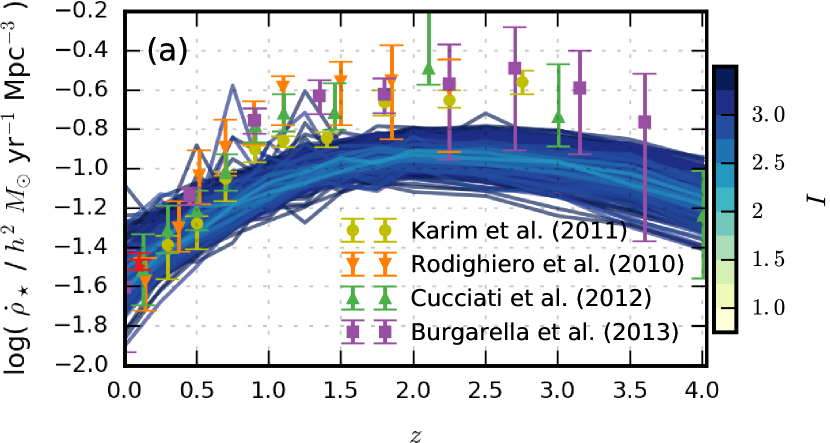
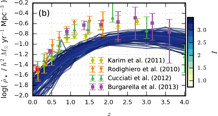
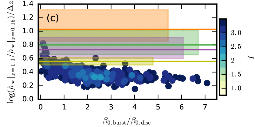
Figure 10: Panels (a) and (b), show the cosmic star formation history (or comoving star formation rate density, SFRD), of runs with $I<3.5$ with respect to the redshifts $z=0.0,\,0.35,\,0.62,\,0.75,\,0.88,\,1.12$ and $1.25$. The colours correspond to their implausibilities as indicated. Observational data from Rodighiero et al. (2010); Karim et al. (2011); Cucciati et al. (2012), and Burgarella et al. (2013). Panel (a) shows only models with $\beta_{0,\text{burst}}>2\,\beta_{0,\text{disc}}$ while the panel (b) shows the case $\beta_{0,\text{burst}}\leq\beta_{0,\text{disc}}$. Panel (c) highlights the slope as a function of the $\beta_{0,\text{burst}}/\beta_{0,\text{disc}}$ ratio with observational constraints shown as shaded areas (same colours as previous panels). While runs with a larger $\beta_{0,\text{burst}}/\beta_{0,\text{disc}}$ display a qualitatively a better fit to the SFRD, they fail to produce the strong increase in SFRD with redshift between $z=0.5$ and $z=1$, despite providing a better match to the GSMF evolution at the same redshift interval (as it can be seen by the colours).

In Fig. 10 we show the evolution of the cosmic star formation rate density (SFRD) for runs with $\beta_{0,\text{burst}}>2\,\beta_{0,\text{disc}}$ (upper panel) and for $\beta_{0,\text{burst}}\leq\beta_{0,\text{disc}}$ (middle panel), in both cases selecting only “acceptable” runs, with $I<3.5$ when conditioned on the full range of GSMF data. A selection of observational data are shown as coloured points. Runs with a larger $\beta_{0,\text{burst}}/\beta_{0,\text{disc}}$ ratio match well the observations for the SFRD at low redshifts ($z\leq 0.5$), but fail to reproduce the steep rise in SFRD with redshift in the interval $0.5<z<1.0$. When runs with $\beta_{0,\text{burst}}\leq\beta_{0,\text{disc}}$ are examined, one finds a stronger redshift evolution of the SFRD, but the normalization is a factor $\sim 3$ off. It should be remembered, however, that the observational data does not measure the star formation rate directly, but requires calibration. This is usually based on Kennicutt (1998). However, a more recent study by Chang et al. (2015) has suggested that this calibration needs revision (for Mid-IR indicators), bringing the observational data into better agreement with the $\beta_{0,\text{burst}}\leq\beta_{0,\text{disc}}$ models. A similar discrepancy was found in the numerical Eagle simulations (Furlong et al., 2015) and other semi-analytic models (Henriques et al. 2015, see also Guo et al. 2016). It is noticeable, however, that these runs – Panel (b) – are generally in less plausible agreement with the mass function data than those in Panel (a).

We quantify these differences more clearly in Panel (c). Here the slope of the star formation rate rate density is plotted as a function of $\beta_{0,\text{burst}}/\beta_{0,\text{disc}}$, with the colour coding indicating the plausibility of the run. The coloured shaded regions indicate the constraints implied by the observational data. The tension between the GSMF and the observed decline in the star formation rate density is now evident. While models require very small ratios of $\beta_{0,\text{burst}}/\beta_{0,\text{disc}}$ to match the SFRD observations, the most plausible models with respect to the GSMF evolution, i.e. those with $I<2.5$, all have $1.66<\beta_{0,\text{burst}}/\beta_{0,\text{disc}}<2.56$.

5 Summary and Conclusions

In this work, using an iterative emulator technique, we explored how the parameter space of galform is constrained by the galaxy stellar mass function. After 6 waves of emulation, using only the local Universe GSMF data, more than $99.9$ per cent of initial volume of the parameter space was deemed too implausible for further exploration and was eliminated. It was possible to find many parameter choices which provide a good match to the local GSMF. The bi-variate projections of this space are shown above the diagonal in Fig. 7. The shape of the GSMF is primarily controlled by parameters related to star formation and feedback, namely: $\alpha_{\text{cool}}$, $\alpha_{\text{hot}}$, $\beta_{0,\text{disc}}$, $\alpha_{\text{reheat}}$, $\nu_{0,\text{sf}}\,$ and $\,f_{\rm stab}$. Constraints on other parameters are weak.

We then included the requirement that the models also match higher redshift data. This parameter space is shown below the diagonal of Fig. 7. This proves to be a much more stringent constraint, and the only acceptable runs found had $I\gtrsim 2$. The high mass end of the GSMF produced by this version of galform is typically too shallow for the local universe and becomes too steep at higher redshifts. This tension is a consequence of the observational data being consistent with small or no increase in the abundance of high mass galaxies between $z>0.35$ and $z=0.0$, compared to the model in which galaxies cannot avoid growing in mass. This tension would still be present even if mass errors had been underestimated by a factor of 2.

In order to better understand the dimensionality and most important variables of the parameter space, we performing a PCA of the non-implausible volume of the parameter space (constrained using the full range of redshifts, Fig. 9). We show that it is possible to write approximate relations between the parameters, expressing conditions which need to be satisfied in order to obtain a model with an acceptable match to the GSMF. Two principal components (i.e. 2 directions in the parameter space) contain most of the information about the basic shape of the GSMF, and these are mainly combinations of the parameters $\alpha_{\text{cool}}$, $\alpha_{\text{hot}}$, $\beta_{0,\text{disc}}$, $\alpha_{\text{reheat}}$, i.e. the parameters controlling feedback processes. The parameters $\nu_{0,\text{sf}}$, $f_{\rm stab}$ are also significantly constrained compared to their initial values.

The PCA analysis provides a simple way to better understand why some model are able to match both the local and high redshift GSMF data (points below the diagonal in Fig. 9), while other models only match the observational at $z=0$ (points above the diagonal in Fig. 9). We show that the primary differences are encoded in Var 15, 16 and (primarily) 17. Models which match the $z=0$ GSMF but not the higher redshift data tend to have higher values of Var 17, and thus lower values of $f_{\rm stab}$ which tends to make disks more unstable at low redshift.

In this paper, we explored a model in which the we allowed the mass loading in starburst (driven by mergers or disk instabilities) to be different from the mass loading in quiescent star formation. The normalization of the quiescent mass, $\beta_{0,\text{disc}}$ loading is strongly constrained, while marginally acceptable models can be found for most of the range of values for the burst mass loading, $\beta_{0,\text{burst}}$. Nevertheless, this does not mean that the full range of $\beta_{0,\text{burst}}$ is equally plausible: there is a much larger density of acceptable models ($I\lesssim 3$) with $20<\beta_{0,\text{burst}}<30$ and the most plausible models, with $I<2.5$, have $1.66<\beta_{0,\text{burst}}/\beta_{0,\text{disc}}<2.56$.

We have deliberately focused the paper on the GSMF. This encoded the star formation history of the Universe, but we can also compare the models to the observed star formation rates of galaxies. We do this by computing the volume averaged star formation rate density in the model. We find that the star formation history is sensitive to the choice of the ratio $\beta_{0,\text{burst}}/\beta_{0,\text{disc}}$. While models with $\beta_{0,\text{burst}}>\beta_{0,\text{disc}}$ offer a reasonable match to the GSMF evolution, they fail to display sufficiently rapid increase in the cosmic SFRD. These results show the important additional information that can be extracted by confronting the constrained models with additional datasets, but that this needs to be done with care, since it is quite possible that systematic differences may make it hard to simultaneously provide a plausible description of all the available data if the observational uncertainites are taken at face value. The apparent contradictions inherent in different datasets must be carefully accounted for: as they may point to missing physics in the model. Clearly a future avenue for further progress is to apply the methods we have developed here to a much wider range of datasets.

Finally, we note that the main aim of this paper has been to examine how information on the formation of galaxies can be extracted from observational dataset. We have shown how simple physical results can emerge from the analysis of a highly complex model. This approach can equally be applied across a wide range of science disciplines where observational data are used to constrain seeming complex numerical models.

Appendix A Details of the History Matching procedure

At each wave a set of 5000 runs were performed using space filling designs based on maximin Latin hypercubes with rejection (see, for example, Sacks et al., 1989; Santner et al., 2003; Currin et al., 1991). Third order polynomials were used as the set of candidate regression terms for $\beta_{ij}g_{ij}(x_{A_{i}})$ in equation (15), with linear model selection based on AIC criteria used to choose both the list of active inputs $x_{A_{i}}$, and the final list of polynomial terms used, for each output labelled by $i$. As we had access to reasonable numbers of runs at each wave we used a vague prior limit for the $\beta_{ij}$ parameters and corresponding OLS estimates for the total residual variance $\sigma_{i}^{2}=\sigma_{u_{i}}^{2}+\sigma_{v_{i}}^{2}$, with $\sigma_{v_{i}}^{2}=\alpha\sigma_{i}^{2}$ where $\alpha$ was chosen so the nugget term represented a small proportion of the total variance, checked using emulator diagnostics (Bastos & O’Hagan, 2008). The correlation lengths were specified to be $\theta_{i}=0.35$, following the argument for the residual of a third order polynomial fit presented by Vernon et al. (2010a). The set of outputs to be used in each wave $Q_{k}$ was chosen by scanning through all possible outputs with approximate linear model regression based emulators, and selecting those that had the highest chance of input space reduction, which were then emulated in detail using equation (15).

Appendix B Full PCA results

Table B shows the full results of the PCA of the volume of the parameter space containing models with $I<3.4$ with respect to redshifts $z=0,\,0.35,\,0.62,\,0.75,\,0.88,\,1.12,\,1.25$ and $1.43$ (which corresponds to 508 runs in our library).

Table 3: Principal component analysis for the acceptable space of galaxy stellar mass functions (see details in the text). Each column shows one PCA variable, ordered here by increasing standard deviation. Small relative standard deviations correspond to components that are tightly constrained by the requirement of producing a good luminosity function. Dominant input variables in each of the vectors are highlighted in bold font. The variables have been ordered so that the most constrained components appear first.

	Mean	Var20	Var19	Var18	Var17	Var16	Var15	Var14	Var13	Var12	Var11
$F_{\rm SMBH}$	0.0357	-0.00148	0.00467	0.0113	-0.0102	-0.0557	0.0538	-0.0076	-0.132	0.35	0.112
$P_{\rm sf}$	-0.0176	-0.0116	0.0118	-0.00198	-0.0417	0.0764	0.0503	0.0777	-0.293	-0.274	-0.134
$V_{\rm cut}$	0.0341	0.00623	0.00514	0.0309	-0.0103	-0.07	0.00895	-0.0931	-0.121	-0.0229	0.0929
$\alpha_{\rm cool}$	0.0647	-0.634	-0.576	-0.229	0.029	-0.322	0.226	0.0426	-0.0754	-0.0283	-0.0785
$\alpha_{\rm hot}$	0.673	0.583	-0.232	-0.604	-0.243	-0.0284	0.404	0.03	0.0473	0.035	-0.00876
$\alpha_{\rm reheat}$	0.462	0.0444	0.356	-0.0815	-0.0894	-0.843	-0.134	0.0222	0.0401	0.212	0.0795
$\alpha_{\rm rp}$	0.14	-0.0193	-0.0123	0.00722	0.064	0.0411	-0.0134	0.2	0.494	-0.0779	0.0525
$\beta_{0,{\rm burst}}$	0.0934	-0.141	-0.157	0.158	-0.0282	0.188	0.164	-0.0453	0.136	0.431	0.357
$\beta_{0,{\rm disk}}$	-0.464	0.401	-0.669	0.26	0.079	-0.172	-0.509	-0.048	-0.0144	0.0534	0.0391
$\beta_{\rm sf}$	-0.0574	0.00181	0.00683	-0.00788	0.071	-0.0104	-0.124	0.222	0.364	0.24	-0.29
$\epsilon_{\rm edd}$	-0.103	0.0123	-0.00878	0.0584	0.0087	-0.089	-0.0217	-0.242	0.175	-0.0872	-0.238
$\epsilon_{\rm strip}$	0.0167	0.0143	0.00422	-0.0143	-0.0706	-0.0291	-0.0867	-0.315	-0.356	0.0492	-0.133
$\nu_{0,{\rm sf}}$	-0.456	0.239	-0.0577	0.613	0.191	-0.244	0.637	0.148	-0.0399	-0.0908	-0.0714
$\tau_{\rm min,burst}$	-0.181	-0.0143	-0.00137	0.063	-0.017	0.0348	0.191	-0.768	0.237	0.247	-0.16
$f_{\rm burst}$	-0.106	0.00122	0.00577	-0.0279	0.0264	0.096	0.017	0.107	0.148	0.23	0.36
$f_{\rm dyn}$	0.062	0.00556	0.00795	0.00359	0.049	0.123	-0.00325	0.216	-0.164	0.432	-0.603
$f_{\rm ellip}$	-0.0319	-0.00621	-0.00332	0.0121	-0.0198	-0.0612	-0.0399	-0.206	0.307	-0.422	-0.0321
$f_{\rm stab}$	-0.362	-0.0922	-0.0586	0.297	-0.931	0.017	-0.0108	0.106	0.0732	-0.00902	-0.0671
$p_{\rm yield}$	-0.175	0.0974	0.0909	0.102	-0.0257	0.0788	-0.0834	-0.0576	-0.222	0.0669	0.0311
$z_{\rm cut}$	-0.0931	-0.00263	-0.000888	0.0131	-0.0299	-0.00443	0.0278	-0.0683	-0.255	0.0149	0.357
Rel. Std. Dev.		0.0707	0.0952	0.174	0.217	0.354	0.361	0.405	0.442	0.461	0.469
	Var10	Var9	Var8	Var7	Var6	Var5	Var4	Var3	Var2	Var1
$F_{\rm SMBH}$	-0.127	0.368	0.431	0.279	-0.175	-0.111	0.349	-0.306	-0.15	-0.381
$P_{\rm sf}$	0.37	-0.422	0.353	0.262	0.39	0.00731	-0.0154	-0.362	-0.111	0.00302
$V_{\rm cut}$	0.534	0.0675	-0.144	0.0874	-0.374	-0.0474	-0.12	0.241	-0.655	-0.0106
$\alpha_{\rm cool}$	-0.0962	-0.0286	-0.113	0.0446	-0.0366	-0.0254	0.0225	-0.0839	-0.0507	0.0843
$\alpha_{\rm hot}$	-0.0202	-0.0176	0.0152	0.0385	-0.0485	0.0562	-0.0579	-0.00184	-0.0117	0.0512
$\alpha_{\rm reheat}$	0.0525	-0.186	0.00651	-0.037	0.0899	0.134	-0.0759	-0.0512	0.0341	-0.0262
$\alpha_{\rm rp}$	-0.2	0.00332	0.215	-0.358	0.164	0.233	0.0666	-0.22	-0.578	0.132
$\beta_{0,{\rm burst}}$	0.0889	-0.246	0.265	0.129	-0.0482	0.436	-0.381	0.147	0.131	-0.0425
$\beta_{0,{\rm disk}}$	0.0519	-0.0732	0.00204	-0.0501	0.0594	-0.0166	0.0345	-0.0425	0.00823	-0.0667
$\beta_{\rm sf}$	0.0626	0.136	0.132	0.349	-0.0256	-0.456	-0.413	-0.0844	0.019	0.328
$\epsilon_{\rm edd}$	0.161	0.0676	0.258	0.22	-0.206	0.35	0.469	0.157	0.15	0.507
$\epsilon_{\rm strip}$	-0.27	0.425	0.0524	0.125	0.449	0.231	-0.307	0.166	-0.237	0.186
$\nu_{0,{\rm sf}}$	-0.0611	0.0929	-0.067	0.0272	0.059	-0.0342	-0.0325	0.0103	-0.00214	0.0434
$\tau_{\rm min,burst}$	0.0595	-0.211	-0.0785	-0.171	0.136	-0.283	0.0462	-0.18	-0.0739	-0.0642
$f_{\rm burst}$	0.221	0.141	-0.523	0.319	0.422	0.0604	0.314	-0.152	-0.0191	0.161
$f_{\rm dyn}$	0.23	0.0689	-0.218	-0.262	-0.0617	0.351	0.00458	-0.22	0.0228	-0.0977
$f_{\rm ellip}$	0.0984	0.289	-0.171	0.225	-0.157	0.322	-0.305	-0.413	0.142	-0.304
$f_{\rm stab}$	-0.000828	0.0418	-0.043	-0.0288	0.00779	-0.0626	0.0502	0.000526	-0.0122	0.00991
$p_{\rm yield}$	-0.473	-0.371	-0.274	0.27	-0.375	0.0953	-0.0405	-0.348	-0.198	0.281
$z_{\rm cut}$	0.229	0.275	0.122	-0.429	-0.14	-0.0977	-0.141	-0.425	0.189	0.456
Rel. Std. Dev.	0.476	0.497	0.507	0.522	0.533	0.542	0.566	0.582	0.596	0.619

Acknowledgements

We thank Cedric Lacey for comments on the paper. LFSR has been supported by STFC (ST/N000900/1 and ST/L005549/1) and acknowledges support from the European Commission’s Framework Programme 7, through the Marie Curie International Research Staff Exchange Scheme LACEGAL (PIRSES-GA-2010-269264). LFSR thanks Jacqueline Dourado and the Federal University of Piauí for the kindness and hospitality during the writing of part of this work. IV gratefully acknowledges MRC (RF060151) and EPSRC (EP/E00931X/1) funding. The research was also supported by the UK Science and Technology Facilities Council (ST/F001166/1 and ST/I000976/1), Rolling and Consolidating Grants to the ICC. This work used the DiRAC Data Centric system at Durham University, operated by the Institute for Computational Cosmology on behalf of the STFC DiRAC HPC Facility (www.dirac.ac.uk). This equipment was funded by BIS National E-infrastructure capital grant (ST/K00042X/1), STFC capital grant (ST/H008519/1), and STFC DiRAC Operations grant (ST/K003267/1) and Durham University. DiRAC is part of the National E-Infrastructure. This research has made use of NASA’s Astrophysics Data System.

References

- Andrianakis et al. (2015) Andrianakis I., Vernon I., McCreesh N., McKinley T., Oakley J., Nsubuga R., Goldstein M., White R., 2015, PLoS Comput Biol., 11, e1003968
- Andrianakis et al. (2016b) Andrianakis I., McCreesh N., Vernon I., McKinley T., Oakley J., Nsubuga R., Goldstein M., White R., 2016b, Journal of Uncertainty Quantification, in submission
- Andrianakis et al. (2016a) Andrianakis I., Vernon I., McCreesh N., McKinley T., Oakley J., Nsubuga R., Goldstein M., White R., 2016a, RSSC, in submission
- Baldry et al. (2012) Baldry I. K., et al., 2012, MNRAS, 421, 621
- Bastian et al. (2010) Bastian N., Covey K. R., Meyer M. R., 2010, ARA&A, 48, 339
- Bastos & O’Hagan (2008) Bastos T. S., O’Hagan A., 2008, Technometrics, 51, 425
- Baugh (2006) Baugh C. M., 2006, Reports on Progress in Physics, 69, 3101
- Behroozi et al. (2013) Behroozi P. S., Wechsler R. H., Conroy C., 2013, ApJ, 770, 57
- Benson (2010) Benson A. J., 2010, Phys. Rep., 495, 33
- Benson (2014) Benson A. J., 2014, MNRAS, 444, 2599
- Blitz & Rosolowsky (2006) Blitz L., Rosolowsky E., 2006, ApJ, 650, 933
- Bower (1991) Bower R. G., 1991, MNRAS, 248, 332
- Bower et al. (2006) Bower R. G., Benson A. J., Malbon R., Helly J. C., Frenk C. S., Baugh C. M., Cole S., Lacey C. G., 2006, MNRAS, 370, 645
- Bower et al. (2010) Bower R. G., Vernon I., Goldstein M., Benson A. J., Lacey C. G., Baugh C. M., Cole S., Frenk C. S., 2010, MNRAS, 407, 2017
- Bruzual & Charlot (2003) Bruzual G., Charlot S., 2003, MNRAS, 344, 1000
- Brynjarsdottir & O’Hagan (2014) Brynjarsdottir J., O’Hagan A., 2014, Inverse Problems, 30, 24
- Burgarella et al. (2013) Burgarella D., et al., 2013, A&A, 554, A70
- Chabrier (2003) Chabrier G., 2003, PASP, 115, 763
- Chang et al. (2015) Chang Y.-Y., van der Wel A., da Cunha E., Rix H.-W., 2015, ApJS, 219, 8
- Cirasuolo et al. (2010) Cirasuolo M., McLure R. J., Dunlop J. S., Almaini O., Foucaud S., Simpson C., 2010, MNRAS, 401, 1166
- Cole et al. (2000) Cole S., Lacey C. G., Baugh C. M., Frenk C. S., 2000, MNRAS, 319, 168
- Craig et al. (1996) Craig P. S., Goldstein M., Seheult A. H., Smith J. A., 1996, in Bernardo J. M., Berger J. O., Dawid A. P., Smith A. F. M., eds, , Bayesian Statistics 5. Clarendon Press, Oxford, UK, pp 69–95
- Craig et al. (1997) Craig P. S., Goldstein M., Seheult A. H., Smith J. A., 1997, in Gatsonis C., Hodges J. S., Kass R. E., McCulloch R., Rossi P., Singpurwalla N. D., eds, , Vol. 3, Case Studies in Bayesian Statistics. SV, New York, pp 36–93
- Cucciati et al. (2012) Cucciati O., et al., 2012, A&A, 539, A31
- Cumming & Goldstein (2009a) Cumming J. A., Goldstein M., 2009a, in O’Hagan A., West M., eds, , Handbook of Bayesian Analysis. Oxford University Press, Oxford, UK
- Cumming & Goldstein. (2009b) Cumming J. A., Goldstein. M., 2009b, Technometrics, 51, 377
- Currin et al. (1991) Currin C., Mitchell T., Morris M., Ylvisaker D., 1991, JASA, 86, 953
- Font et al. (2008) Font A. S., et al., 2008, MNRAS, 389, 1619
- Furlong et al. (2015) Furlong M., et al., 2015, MNRAS, 450, 4486
- Geyer (2011) Geyer C., 2011, Handbook of Markov Chain Monte Carlo. CRC press, pp 3–48
- Goldstein (1999) Goldstein M., 1999, in Kotz S., et al., eds, , Encyclopaedia of Statistical Sciences. Wiley, pp 29–34
- Goldstein & Rougier (2009) Goldstein M., Rougier J. C., 2009, JSPI, 139, 1221
- Goldstein & Wooff (2007) Goldstein M., Wooff D. A., 2007, Bayes Linear Statistics: Theory and Methods. Wiley, Chichester
- Goldstein et al. (2013) Goldstein M., Seheult A., Vernon I., 2013, Environmental Modelling: Finding Simplicity in Complexity, second edn. John Wiley & Sons, Ltd, Chichester, UK, doi:10.1002/9781118351475.ch26
- Gonzalez-Perez et al. (2014) Gonzalez-Perez V., Lacey C. G., Baugh C. M., Lagos C. D. P., Helly J., Campbell D. J. R., Mitchell P. D., 2014, MNRAS, 439, 264
- Guo et al. (2013) Guo Q., White S., Angulo R. E., Henriques B., Lemson G., Boylan-Kolchin M., Thomas P., Short C., 2013, MNRAS, 428, 1351
- Guo et al. (2016) Guo Q., et al., 2016, MNRAS, 461, 3457
- Heckman et al. (1990) Heckman T. M., Armus L., Miley G. K., 1990, ApJS, 74, 833
- Heitmann et al. (2009) Heitmann K., Higdon D., et al., 2009, Astrophys. J., 705, 156
- Henderson et al. (2009) Henderson D. A., Boys R. J., Krishnan K. J., Lawless C., Wilkinson D. J., 2009, Journal of the American Statistical Association, 104, 76
- Henriques et al. (2009) Henriques B. M. B., Thomas P. A., Oliver S., Roseboom I., 2009, MNRAS, 396, 535
- Henriques et al. (2013) Henriques B. M. B., White S. D. M., Thomas P. A., Angulo R. E., Guo Q., Lemson G., Springel V., 2013, MNRAS, 431, 3373
- Henriques et al. (2015) Henriques B. M. B., White S. D. M., Thomas P. A., Angulo R., Guo Q., Lemson G., Springel V., Overzier R., 2015, MNRAS, 451, 2663
- Higdon et al. (2004) Higdon D., Kennedy M., Cavendish J. C., Cafeo J. A., Ryne R. D., 2004, SIAM Journal on Scientific Computing, 26, 448
- Kampakoglou et al. (2008) Kampakoglou M., Trotta R., Silk J., 2008, MNRAS, 384, 1414
- Karim et al. (2011) Karim A., et al., 2011, ApJ, 730, 61
- Kennedy & O’Hagan (2001) Kennedy M. C., O’Hagan A., 2001, JRSSB, 63, 425
- Kennicutt (1983) Kennicutt Jr. R. C., 1983, ApJ, 272, 54
- Kennicutt (1998) Kennicutt Jr. R. C., 1998, ApJ, 498, 541
- Komatsu et al. (2011) Komatsu E., Smith K. M., Dunkley J., Bennett C. L., Gold B., Hinshaw G., Jarosik N., et al. 2011, ApJS, 192, 18
- Kriek et al. (2009) Kriek M., van Dokkum P. G., Labbé I., Franx M., Illingworth G. D., Marchesini D., Quadri R. F., 2009, ApJ, 700, 221
- Lacey & Cole (1993) Lacey C., Cole S., 1993, MNRAS, 262, 627
- Lacey et al. (2016) Lacey C. G., et al., 2016, MNRAS, 462, 3854
- Lagos et al. (2011) Lagos C. D. P., Lacey C. G., Baugh C. M., Bower R. G., Benson A. J., 2011, MNRAS, 416, 1566
- Lagos et al. (2012) Lagos C. D. P., Bayet E., Baugh C. M., Lacey C. G., Bell T. A., Fanidakis N., Geach J. E., 2012, MNRAS, 426, 2142
- Lagos et al. (2014) Lagos C. d. P., Davis T. A., Lacey C. G., Zwaan M. A., Baugh C. M., Gonzalez-Perez V., Padilla N. D., 2014, MNRAS, 443, 1002
- Li & White (2009) Li C., White S. D. M., 2009, MNRAS, 398, 2177
- Lu et al. (2014) Lu Y., Mo H. J., Lu Z., Katz N., Weinberg M. D., 2014, MNRAS, 443, 1252
- Malbon et al. (2007) Malbon R. K., Baugh C. M., Frenk C. S., Lacey C. G., 2007, MNRAS, 382, 1394
- Martin et al. (2012) Martin C. L., Shapley A. E., Coil A. L., Kornei K. A., Bundy K., Weiner B. J., Noeske K. G., Schiminovich D., 2012, ApJ, 760, 127
- McCarthy et al. (2008) McCarthy I. G., Frenk C. S., Font A. S., Lacey C. G., Bower R. G., Mitchell N. L., Balogh M. L., Theuns T., 2008, MNRAS, 383, 593
- Mitchell et al. (2013) Mitchell P. D., Lacey C. G., Baugh C. M., Cole S., 2013, MNRAS, 435, 87
- Mitchell et al. (2016) Mitchell P. D., Lacey C. G., Baugh C. M., Cole S., 2016, MNRAS, 456, 1459
- Muzzin et al. (2013) Muzzin A., et al., 2013, ApJ, 777, 18
- O’Hagan (2006) O’Hagan A., 2006, Reliability Engineering and System Safety, 91, 1290
- Parkinson et al. (2008) Parkinson H., Cole S., Helly J., 2008, MNRAS, 383, 557
- Pukelsheim (1994) Pukelsheim F., 1994, AmerStat, 48, 88
- R (2015) R 2015, R: A Language and Environment for Statistical Computing. R Foundation for Statistical Computing, Vienna, Austria, http://www.R-project.org/
- Rodighiero et al. (2010) Rodighiero G., et al., 2010, A&A, 518, L25
- Sacks et al. (1989) Sacks J., Welch W. J., Mitchell T. J., Wynn H. P., 1989, Statistical Science, 4, 409
- Santner et al. (2003) Santner T. J., Williams B. J., Notz W. I., 2003, The Design and Analysis of Computer Experiments. SV, New York
- Smith et al. (2015) Smith R. J., Lucey J. R., Conroy C., 2015, MNRAS, 449, 3441
- Somerville & Davé (2015) Somerville R. S., Davé R., 2015, ARA&A, 53, 51
- Tomczak et al. (2014) Tomczak A. R., et al., 2014, ApJ, 783, 85
- Vernon et al. (2010a) Vernon I., Goldstein M., Bower R. G., 2010a, Bayesian Analysis, 5, 619
- Vernon et al. (2010b) Vernon I., Goldstein M., Bower R. G., 2010b, Bayesian Analysis, 5, 697
- Vernon et al. (2014) Vernon I., Goldstein M., Bower R. G., 2014, Statistical Science, 29, 81
- Williamson et al. (2013) Williamson D., Goldstein M., Allison L., Blaker A., Challenor P., Jackson L., Yamazaki K., 2013, Climate Dynamics, 41, 1703