Dark Energy and Dark Matter in a Model of an Axion Coupled to a Non-Abelian Gauge Field

Abstract

We study cosmological field configurations (solutions) in a model in which the pseudo-scalar phase of a complex field couples to the Pontryagin density of a massive non-abelian gauge field, in analogy to how the Peccei-Quinn axion field couples to the $SU(3)$-color gauge field of QCD. Assuming that the self-interaction potential of the complex scalar field has the typical Mexican hat form, we find that the radial fluctuations of this field can act as Dark Matter, while its phase may give rise to tracking Dark Energy. In our model, Dark-Energy domination will, however, not continue for ever. A new component of dark matter, namely the one originating from the gauge field, will dominate in the future.

I Introduction

Current observations Planck2015 show that about $95\%$ of the energy in the universe does not come from visible matter observed in ordinary laboratory experiments, but from a new kind of matter in the form of Dark Energy and Dark Matter. Evidence for Dark Matter and Dark Energy comes exclusively from gravitational effects: Dark Matter was first introduced to account for the missing mass in galaxies Zwicky ; Rubin and galaxy clusters. Dark Matter has the same gravitational interactions and produces the same gravitational effects as regular matter in the form of a pressure-less gas, but it interacts only very weakly with visible matter and photons. The presence of Dark Matter is required in order to obtain the observed agreement between the angular power spectrum of cosmic microwave background (CMB) fluctuations and the power spectrum of density fluctuations; (see, e.g., RHBrev for a discussion of this point). As compared to Dark Matter, far less is known about Dark Energy. Its presence in the cosmos is required to explain the apparent accelerated expansion of the Universe, as inferred from Supernova observations Perlmutter ; Riess , and to reconcile the spatial flatness of the Universe, as derived from CMB anisotropy measurements Planck2015 , with the total energy density due to matter, including Dark Matter, inferred from the observed dynamics of galaxies and galaxy clusters.

In order to explain the data provided by these observations, the equation-of-state parameter $w$ of Dark Energy (namely the ratio of pressure to energy density) is now known to be close to $w=-1$. Dark Energy could be due to a cosmological constant in Einstein’s field equation of the general theory of relativity. It could also be a manifestation of modified laws of gravity, which become manifest only on cosmological scales. Or Dark Energy could be caused by a new matter field (“quintessence field”) with an unusual equation of state, $w\simeq-1$; (see, e.g., DEreviews for recent reviews on the Dark Energy puzzle). In this paper we focus our attention on the third scenario, which we call the quintessence approach; (see quintessence for some original references).

A fairly popular candidate axionDM for Dark Matter is the invisible axion axion ; invisible , a very light pseudo-scalar field originally introduced to solve the strong CP problem of quantum chromodynamics (QCD) PQ . This axion field couples linearly to the instanton (Pontryagin) density of the $SU(3)$-color gauge field of QCD; (it plays the role of a dynamical vacuum angle). If the VEV of the axion field can be shown to vanish the strong CP problem of QCD is solved.

It has been postulated recently us that Dark Energy could arise from another pseudo-scalar field, a new axion, that couples linearly to the Pontryagin density of a heavy non-abelian gauge field operating at a high energy scale. The new axion could be conjugate to an anomalous current, $j^{\mu}_{\ell}$, that couples to the gauge field; see, e.g., Weinberg . The chiral anomaly would then explain why the axion couples to the Pontryagin density of the gauge field. (One might speculate that the anomalous current is leptonic and the gauge field is the weak $SU(2)$-gauge field.)

One of the challenges in the quintessence approach is to explain why Dark Energy is becoming dynamically important around the present time, and not already in the very early universe, or in the remote future. If a cosmological constant were to be the source of Dark Energy we would be faced with the problem of explaining the precise, very small value that the cosmological constant would have to be given in order to explain the observational data. In our quintessence approach to Dark Energy we want to avoid to be forced to introduce a comparably tiny number by hand. Tracking Quintessence tracking is a way to cope with this problem. In models of tracking quintessence, the energy density of the field responsible for Dark Energy follows the energy density of the dominant matter field until times when a dynamical crossover prevents further decline of its energy density, and Dark Energy becomes the dominant form of energy in the Universe. In us we have observed that the coupling of an axion to the Pontryagin density of a massive non-Abelian gauge field can cause slow rolling of the axion field, so that, as a consequence, the equation of state of the axion field is the one required of Dark Energy, and this has yielded an interesting scenario of tracking quintessence.

In this paper, we introduce a toy model of a complex field whose phase (angular component) plays the role of a pseudo-scalar axion that is linearly coupled to the instanton density of a massive non-abelian gauge field. This gauge field is invisible below rather high energy scales. Our model appears to describe, at once, Dark Matter and Dark Energy. Both the radial and the angular components of the complex scalar field describe dynamical degrees of freedom. While the radial component leads to Dark Matter, its phase is a source of Dark Energy; (tracking quintessence).

If the coupling of the axion to the instanton density of the gauge field were neglected our model would yield a renomalizable quantum field theory, in contrast to the model studied in us .

The organization of this paper is as follows: In the next section we introduce our model and derive its field equations (of motion). In Section 3 we discuss cosmological solutions of the classical field equations, assuming that the fields only depend on cosmological time. We show how the radial component of the scalar field can play the role of Dark Matter, whereas its phase is a candidate for Dark Energy, for reasons similar to those advanced in us . A discussion section concludes our paper.

The following notations and units will be used throughout: the cosmological scale factor is denoted by $a(t)$, $z(t)$ is the associated cosmological redshift, and the Hubble expansion rate by $H(t)$; space-time indices are denoted by Greek letters, group indices by latin letters; and we use natural units in which the speed of light, $c$, and Planck’s constant, $\hbar$, are set to $1$.

II The Model

We consider a complex scalar field $\varphi$ with Lagrangian density

$${\cal L}\,=\,\frac{1}{2}\partial_{\mu}\overline{\varphi}\partial^{\mu}\varphi-\frac{\lambda}{2}\bigl{(}|\varphi|^{2}-R_{0}^{2}\bigr{)}^{2}-\frac{\mu^{2}}{2}|\varphi-{\bar{\varphi}}|^{4},$$ (1)

where $\lambda$ and $\mu$ are dimensionless coupling constants. This Lagrangian describes a renormalizable theory . For $\mu^{2}=0$, the potential for $\varphi$ has the usual “Mexican hat” shape, with ground states breaking the $U(1)$-symmetry of global phase transformations. The modulus of the field minimizing the potential is denoted by $R_{0}$. The term $\propto\mu^{2}$ breaks the $U(1)$- symmetry explicitly; ($U(1)$- symmetry breaking is also encountered in the usual model of the Peccei-Qinn scalar in QCD).

We introduce polar coordinates in field space, i.e., radial and angular components of $\varphi$,

$$\varphi\, = \,Re^{i\theta},$$ (2)

$$R\, = \,R_{0}+r\,,$$

where $\theta$ is the angular component (the phase) of $\varphi$, $R$ its radial component, and $r$ parametrizes radial fluctuations of $\varphi$ about a ground state configuration for $\mu^{2}=0$ corresponding to $|\varphi|=R_{0}$.

If the field $\varphi$ plays a role similar to the one the Peccei-Quinn scalar plays in QCD then it must be coupled linearly to the Pontryagin density of some gauge field, $A_{\mu}^{a}$, which we here take to be a massive non-abelian gauge field effective at a high energy scale. The coupling between the phase, $\theta$, of $\varphi$ and the gauge field $A_{\mu}^{a}$ is described by the following term in the Lagrangian density of the theory

$${\cal L}_{P}\,=\,-\alpha\theta F_{a\mu\nu}{\tilde{F}}_{a}^{\mu\nu}\,.$$ (3)

Here $F_{a\mu\nu}$ is the field strength of $A_{\mu}^{a}$, $\mu$ and $\nu$ are space-time indices, while $a$ is a (gauge) group index, and $\alpha$ is a dimensionless coupling constant.

Besides the field $\varphi$, we introduce an axial chemical potential $\mu_{5}$ conjugate to an axial vector current $J_{\mu}^{5}$ that couples to the gauge field $A_{\mu}^{a}$. The chiral anomaly is expressed by the equation

$$\partial_{\mu}J_{\mu}^{5}\,=\,\frac{2{\tilde{\alpha}}}{\pi}{\rm tr}({\vec{E}}\cdot{\vec{B}})+\text{terms}\propto\text{masses}\,,$$ (4)

where $\tilde{\alpha}$ is a coupling constant. The axial chemical potential conjugate to $J_{\mu}^{5}$ appears in a term ${\cal L}_{Q}$ in the effective Lagrangian for the gauge field analogous to (3), namely

$${\cal L}_{Q}\,=\,-{\tilde{\alpha}}\chi F_{a\mu\nu}{\tilde{F}}_{a}^{\mu\nu}\,,$$ (5)

with

$${\dot{\chi}}\,=\,\mu_{5}\,.$$ (6)

In the Appendix we discuss a possible origin of the (dimensionless) pseudo-scalar field $\chi$.

If all spatial gradient terms are neglected the Lagrangian for $\varphi$ becomes

$${\cal L}\, = \,\frac{1}{2}\bigl{(}{\dot{r}}^{2}+R_{0}^{2}{\dot{\theta}}^{2}+2R_{0}r{\dot{\theta}}^{2}+r^{2}{\dot{\theta}}^{2}\bigr{)}$$

$$-\frac{\lambda}{2}\bigl{(}2R_{o}r+r^{2}\bigr{)}^{2}$$

$$-8\mu^{2}\bigl{(}R_{0}^{4}+4R_{0}^{3}r+6R_{0}^{2}r^{2}+4R_{0}r^{3}+r^{4}\bigr{)}{\rm sin}^{4}\theta$$

$$+\alpha\,\theta\,E\cdot B\,,$$

where $E_{a}$ and $B_{a}$ are the electric and magnetic components of the field tensor of the gauge field $A_{\mu}^{a}$, and

$$E\cdot B:=\text{tr}(E\cdot B)=\sum_{i,a}E_{i}^{a}\,B_{i}^{a}.$$

We assume that this gauge field acquires a large mass at a phase transition occuring at an early time denoted $t_{m}$.

In the following, the gauge group is chosen to be $SU(2)$. We make the following ansatz of a homogeneous gauge field configuration, expressed in terms of a scalar field $\psi(t)$ (see e.g. chromo ):

$$A_{0}^{a}(t)\, = \,0,$$ (8)

$$A_{i}^{a}(t)\, = \,a(t)\psi(t)\delta_{i}^{a}\,,$$ (9)

where $\delta_{i}^{a}$ is the Kronecker delta function. The “electric field” $E_{i}^{a}$ is then given by

$$E_{i}^{a}(t)\,\sim\,a^{-1}(a\psi)^{\cdot}\delta_{i}^{a}$$ (10)

and the “magnetic field” by

$$B_{i}^{a}(t)\,\sim\,g(a(t)\psi(t))^{2}\,,$$ (11)

where $g$ is the coupling constant of the non-abelian gauge theory. In the following we will drop the group index. Note that the amplitude of the magnetic field is suppressed, as compared to the one of the electric field, by the gauge coupling constant $g$ (which, later, we will take to be $g\ll 1$) and by an additional factor of $a\psi$.

The field equations of motion for the components of the scalar field $\varphi(t)$ and for $\psi(t)$ (or, equivalently, for the fields $\varphi$ and $E\cdot B$) describing a homogeneous and isotropic cosmology can be derived from the Lagrangian (II) to which the standard Yang-Mills Lagrangian for $A_{\mu}$ is added. We are interested in solutions of the field equations describing small oscillations of $R$ about its ground state value $R=R_{0}$ and the response of the axion field $\theta$ to the gauge field $A_{\mu}$, as determined by its coupling to the Pontryagin term tr($E\cdot B$). We thus linearize the field equations in $r/R_{0}$, and we will later assume that $\theta$ remains so small that we can approximate ${\rm sin}\theta$ by $\theta$. The radial equation of motion then becomes

$${\ddot{r}}+3H{\dot{r}}-R_{0}{\dot{\theta}}^{2}+32R_{0}^{3}\mu^{2}{\rm sin}^{4}\theta+4\lambda R_{0}^{2}r\,=\,0\,,$$ (12)

and the angular equation is given by

$${\ddot{\theta}}+3H{\dot{\theta}}+2\frac{{\dot{r}}}{R_{0}}{\dot{\theta}}+32\mu^{2}R_{0}^{2}{\rm sin}^{3}\theta{\rm cos}\theta\,=\,8\alpha R_{0}^{-2}E\cdot B\,,$$ (13)

where we have kept the ${\dot{r}}/R_{0}$ term, since the term ${\dot{r}}/r$ will be parametrically larger than $H$.

III Cosmological Solutions

We follow the approach outlined in us and search for solutions in which the terms $\propto\dot{\theta},\ddot{\theta}$ in Eq. (13) can be neglected, so that this equation reduces to

$$32\mu^{2}R_{0}^{2}{\rm sin}^{3}\theta{\rm cos}\theta\,\simeq\,8\alpha R_{0}^{-2}E\cdot B\,.$$ (14)

Note that this relation between the axion field and the instanton density is identical to the one used in chromo ; sorbo ; shahin to derive slow-rolling of an inflaton field at sub-Planckian field values. In the small $\theta$ approximation Eq. (14) reduces to

$$\theta^{3}\,\simeq\,\frac{1}{4}\alpha\mu^{-2}R_{0}^{-4}E\cdot B\,.$$ (15)

The solutions of the radial field equation we are looking for describe small oscillations of $R$ about its ground state value, i.e., oscillations of $r$ about $0$. Assuming that $\theta$ is a solution of (15) and that $E\cdot B$ decays like an inverse power of time, the leading terms in the radial equation yield the equation

$${\ddot{r}}+3H{\dot{r}}+4\lambda R_{0}^{2}r\,=\,0\,,$$ (16)

which describes the motion of a damped harmonic oscillator. To solve (16) we make the ansatz

$$r(t)\,\equiv\,x(t)e^{\sigma(t)}\,,$$ (17)

where $x$ and $\sigma$ are two real-valued functions of time $t$, with $\sigma$ chosen such that terms $\propto\dot{x}$ in (16) cancel. This requirement implies that

$${\dot{\sigma}}\,=\,-\frac{3}{2}H\,,$$ (18)

The radial equation then reduces to

$${\ddot{x}}+\bigl{(}4\lambda R_{0}^{2}-\frac{9}{4}H^{2}-\frac{3}{2}{\dot{H}}\bigr{)}x\,=\,0\,.$$ (19)

Except at the beginning of the evolution of the Universe, the terms $\propto H^{2}$ and $\dot{H}$ in the frequency are negligible, and the solutions, $x(t)$, of (19) describe harmonic oscillations about $x=0$ with frequency, $\omega$, given by

$$\omega\,=\,2\sqrt{\lambda}R_{0}\,.$$ (20)

This is the mass of our dark matter candidate. Note that, even at the beginning of the evolution, this mass is larger than $H$ by a factor proportional to $R_{0}/m_{pl}$ (where $m_{pl}$ is the Planck mass), as follows from the Friedmann equation for $H$.

At this point we must verify that it is self-consistent to neglect the terms in the original angular and radial equations of motion that we have omitted in (15) and (16). We first consider the angular equation of motion. We temporarily omit all coupling constants and factors of order unity from our equations. The terms ${\ddot{\theta}}$ and $3H{\dot{\theta}}$ are both of the order $O(H^{2}\text{ }\theta)$. The terms, denoted $T$, we have kept in the angular equation scale as

$$T\,\sim\,R_{0}^{2}\frac{E\cdot B}{\rho_{R}}\,,$$ (21)

where $\rho_{R}\equiv R_{0}^{4}$, whereas

$$H^{2}\theta\,\sim\,H^{2}\bigl{(}\frac{E\cdot B}{\rho_{R}}\bigr{)}^{1/3}\,.$$ (22)

At the initial time, $E\cdot B\sim\rho_{R}$. Thus, the ${\ddot{\theta}}$- and $3H{\dot{\theta}}$- terms are suppressed, initially, as compared to the terms we have kept, by the square of the factor $H/R_{0}$. The Friedmann equations imply that this factor is of order $O(R_{0}/m_{pl})$, which is expected to be tiny. Furthermore, as functions of time, the terms ${\ddot{\theta}}$ and $3H{\dot{\theta}}$ decay faster than $T$. Hence, it is self-consistent to neglect the ${\ddot{\theta}}$- and $3H{\dot{\theta}}$- terms in Eq. (13).

In a similar way one may check that the term $2\,{\dot{r}}{\dot{\theta}}/R_{0}$ in (13) is negligible: Inserting the expression (15) for $\theta$ into (13), comparison between this term and the ones we have kept yields the condition

$$Hr\,<\,R_{0}^{2}\bigl{(}\frac{E\cdot B}{\rho_{R}}\bigr{)}^{2/3}$$ (23)

for the term $\propto{\dot{r}}$ in (13) to be negligible. At the initial time, the left-hand side of (23) is suppressed, as compared to the right-hand side, by one power of $R_{0}/m_{pl}$. Neglecting the decrease in the amplitude of oscillation of $r$, both terms would scale in the same way as a function of time. But since $r$ exhibits a damped oscillation, the left-hand side decreases faster in time than the right-hand side. Hence, our approximation (15) for the angular equation (13) is self-consistent.

It is easy to see that neglecting the terms depending on $\theta$ in the radial equation (12) is self-consistent. We leave it to the reader to check this.

As will be shown in the following section, in the absence of any back-reaction of the scalar fields (and/or other matter fields) on the gauge fields, one does not obtain a successful scenario for tracking quintessence: the energy density in $\theta$ will never increase relative to that in regular matter and radiation. However, both the coupling of the scalar field to the Pontryagin density and the term proportional to the extra axial chemical potential that we have introduced in the Lagrangian affect the time evolution of the Pontryagn density ${\vec{E}}\cdot{\vec{B}}$ and make it decrease in time less rapidly than if those terms were absent.

The back-reaction of the scalar field on the gauge field can be analyzed by following the analysis in our previous paper. In the presence of the axion $\theta$ and of the chemical potential $\mu_{5}$, the equation of motion for the electric field has a term proportional to $(\alpha\dot{\theta}+{\tilde{\alpha}}\mu_{5})B$,

$${\dot{E}}+\kappa HE\,=\,-\bigl{(}\alpha{\dot{\theta}}+{\tilde{\alpha}}\mu_{5}\bigr{)}B\,,$$ (24)

where the constant $\kappa$ depends on whether the gauge field has acquired a mass, or not, and whether we are in the radiation or matter epochs. For a massive gauge field in the radiation era, $\kappa=3/2$, which, in the absence of coupling to the axion, i.e., for $\alpha=0$, leads to the scaling characteristic of matter

$$E^{2}(t)\,\sim\,a(t)^{-3}\,.$$ (25)

The equations for $E$ and $B$ are equivalent to a second order differential equation for the scalar function $\psi$, an equation given in chromo .

Treating the right hand side of (24) as a small perturbation, the solution of Eq. (24), given initial conditions at some time $t_{i}$, can be found in first-order Born approximation. It is given by

$$E(t)\,=\,E_{0}(t)\bigl{[}1+\int_{t_{i}}^{t}dt^{`}E_{0}(t^{`})^{-1}S(t^{`})\bigr{]}\,\equiv\,E_{0}+E_{1}\,,$$ (26)

where $E_{0}(t)$ is the solution describing a “free” $E$- field, and

$$S(t^{`})\,=\,\bigl{(}\alpha{\dot{\theta}}(t^{`})+{\tilde{\alpha}}\mu_{5}\bigr{)}B(t^{`})\,.$$ (27)

The “electric field” $E(t)$ can also be written as

$$E(t)\,=\,E_{0}(t)\bigl{[}1+G(t)\bigr{]}\,,$$ (28)

where the factor $G(t)$ is called secular growth factor. This result also follows from the second order differential equation for $\psi(t)$, see us ,

$$\psi(t)\,\sim\psi_{0}(t)\bigl{[}1+G(t)\bigr{]}\,,$$ (29)

where $\psi_{0}(t)$ is the solution found by setting $\alpha$ and ${\tilde{\alpha}}$ to $0$, which corresponds to the field $E_{0}(t)$. Since $E$ is linear in $\psi$ and $B$ is quadratic in $\psi$, both “electric” and “magnetic” fields acquire a secular growth correction linear in $G(t)$, as long as $G(t)<1$. The secular growth term $E_{1}$ will begin to dominate over the background term $E_{0}$ at some time $t_{sec}$ which we want to lie in the interval $t_{eq}<t_{sec}<t_{0}$. Once the secular term starts to dominate over the background term, i.e., when $G(t)>1$, the quantity $E^{2}$ scales as $G^{2}(t)$, $E\cdot B$ scales as $G^{3}$ and $B^{2}$ as $G^{4}$. We must make sure that, at the present time, the quintessence field energy density, which scales as $G^{3}$, dominates over the energy density of the new gauge field, which is proportional to $E^{2}+B^{2}$ (+ a term proportional to the mass of the gauge field) and scales as $G^{4}$. This will only be the case if the constant $\alpha$ is sufficiently large. (The order of magnitude of this constant will be discussed later).

The second term on the right hand side of (26) leads to an extra contribution to $E\cdot B$. In our previous model this term had logarithmic growth in time relative to the term present when the coupling between scalar and gauge field is absent. Hence there will be a time, denoted $t_{sec}$, when the second term begins to dominate over the first, and we have shown that, for $t\gg t_{sec}$, the new term can come to dominate, yielding a tracking Dark Energy model. A constraint on the viability of every such model is that

$$t_{eq}<t_{sec}<t_{0}\,,$$ (30)

where $t_{0}$ is the present time.

In our present model the contribution to the source $S(t)$ originating from the axion decays too rapidly in time to yield a significant growth factor. This is the reason why we have introduced the extra axial chemical potential $\mu_{5}$.

Let us assume that $\mu_{5}$ is constant in time. Then

$$\frac{E_{1}}{E_{0}}(t)\,\sim\,{\tilde{\alpha}}\mu_{5}(t-t_{i})\,,$$ (31)

and the time, denoted $t_{sec}$, when $E_{1}$ starts to dominate and the secular growth sets in is given by

$$t_{sec}\,\sim\,{\tilde{\alpha}}^{-1}\mu_{5}^{-1}\,.$$ (32)

As will be shown in the next section, a necessary condition for a successful tracking dark energy scenario is

$$t_{eq}\,<\,t_{sec}\,<\,t_{0}\,.$$ (33)

Hence we must choose a tiny axial chemical potential $\mu_{5}$ satisfying

$$t_{0}^{-1}\,<\,\tilde{\alpha}\mu_{5}\,<\,t_{sec}^{-1}\,.$$ (34)

This condition could be met naturally if the axial chemical potential redshifts, as the universe expands, until some late time, denoted by $t_{chem}$, with $t_{chem}<t_{eq}$. An idea about a possible origin of such a chemical potential is sketched in Appendix A.

IV Cosmological Scenario

We propose to interpret the radial component, $r$, of the field $\varphi$ as a component of Dark Matter and the angular component, $\theta$, of $\varphi$ as describing Dark Energy. Since the potential for $r$ is close to a quadratic potential of a harmonic oscillator, $r$ performs damped oscillations about $r=0$. This implies that its equation of state is that of cold dark matter, i.e., $w\equiv p/\rho=0$, where $p$ and $\rho$ are pressure and energy density, respectively. Since

$$\rho_{r}(t)\,\sim\,r^{2}(t)\,,$$ (35)

it is easy to check from (18) and (17) that, in the radiation epoch as well as in the matter epoch,

$$\rho_{r}(t)\,\sim\,a(t)^{-3}\,,$$ (36)

which is the scaling that cold dark matter has.

In the following, the contributions of the degrees of freedom described by the fields $r$ and $\theta$ to the total energy density of the Universe are studied. We use the standard notation

$$\Omega_{X}\,=\,\frac{\rho_{X}}{\rho_{0}}\,.$$ (37)

Here, $\Omega_{X}$ is the fraction of the total energy density the substance $X$ contributes to the total energy density, denoted by $\rho_{0}$, of a spatially flat universe.

Since $\Omega_{DM}$, corresponding to Dark Matter, scales as $\Omega_{m}$, corresponding to regular matter, for all times, the coincidence condition that, at the present time, the magnitude of $\Omega_{DM}$ is comparable to the magnitude of the fraction, $\Omega_{B}$, of the total energy density contributed by baryons is a consequence of a similar condition assumed to hold at the time when the Standard Model matter fields acquire their mass. This happens at a temperature $T\equiv T_{EW}\sim 250{\rm GeV}$.

Assuming that the spontaneous breaking of our new “Peccei-Quinn-like” symmetry takes place at a temperature $T_{m}$ (corresponding to a time denoted by $t_{m}$) lower than $T_{EW}$, the condition that will guarantee the right magnitude of the energy density of Dark Matter is given by

$$\Omega_{DM}(T_{m})\,\sim\,\frac{T_{eq}}{T_{m}}\,,$$ (38)

assuming that the degrees of freedom described by the field $r$ do not decay into other degrees of freedom, (an assumption whose validity is examined in Appendix B). In (38), $T_{eq}\sim 3{\rm eV}$ is the temperature at the time, $t_{eq}$, of equal matter and radiation when $\Omega_{B}\sim 1$. The ratio in Eq. (38) is of the order of $10^{-11}$ if $T_{m}\simeq T_{EW}$. This initial condition can be realized if the number density of $r$ is suppressed as compared to the number density of photons in the same way as the baryon number.

The radial component $r$ starts to oscillate after the breaking of the new symmetry. The temperature at which this symmetry breaking occurs is

$$T_{c}\,\sim\,R_{0}\,.$$ (39)

This can be inferred from the following argument: There are finite-temperature corrections to the potential of the scalar field, the leading such corrections being given by Dolan

$$\Delta V\,\sim\,g^{2}T^{2}|\varphi|^{2}\,,$$ (40)

where $g$ is a typical coupling constant. Invoking naturalness we expect $g^{2}\sim\lambda$; (see, e.g., RMP for a review of these arguments in the context of cosmology). In (39), $T_{c}$ is the temperature where the negative contributions to the quadratic term in the potential, expanded about $\varphi=0$, cancel the positive contribution from $\Delta V$. This implies (39). In the following, we will assume that $T_{c}=T_{m}$.

The energy density stored in the $r$ degrees of freedom at the time of the phase transition is proportional to the potential energy density before the phase transition, i.e.,

$$\rho_{DM}(T_{c})\,\sim\,\lambda R_{0}^{4}\,,$$ (41)

while the critical energy density is

$$\rho_{rad}\,\sim\,T_{c}^{4}\,.$$ (42)

Hence

$$\Omega_{DM}(T_{c})\,\sim\,\lambda\,.$$ (43)

Comparing (38) with (43), we see that there is a curve in the $(R_{0},\lambda)$ parameter plane leading to the Dark Matter density observed today . Note that, as in the case of the QCD axion as a candidate for Dark Matter, the mass of the field quanta of the $r$- field is not determined uniquely by the requirement that we obtain the Dark Matter density observed today. What is determined is a combination of the coupling constant $\lambda$ and the Dark Matter particle mass, $\omega$, which must be given by

$$\omega\,\sim\,\lambda^{-1/2}T_{eq}\,.$$ (44)

Next, we study the equation of state of the degrees of freedom described by the axion field $\theta$. Its potential energy density, $V$, is given by

$$V(\theta)\,\simeq\,8\mu^{2}R_{0}^{4}\theta^{4},$$ (45)

whereas the kinetic energy density, $K$, is given by

$$K(\theta)\,\sim\,{\dot{\theta}}^{2}H^{2}R_{0}^{2}\theta^{2}\,.$$ (46)

Inserting the slow-roll solution (15), one easily finds that

$$\frac{K}{V}\,\sim\,\bigl{(}\frac{R_{0}}{m_{pl}}\bigr{)}^{4/3}\,.$$ (47)

Thus, the equation of state parameter $w_{\theta}$ of the axion field $\theta$ is

$$w_{\theta}\,\simeq\,-1,$$ (48)

and hence $\theta$ gives rise to Dark Energy.

It remains to show that, in fact, $\theta$ gives rise to tracking Dark Energy, i.e., its contribution to the total energy density $\rho_{0}(t)$ tracks the contribution of the dominant component of matter until some late time.

First, we infer from (45) and (15) that the energy density of $\theta$ (which is dominated by the potential energy density) is given by

$$\rho_{\theta}(t)\,\simeq\,2\alpha\bigl{(}\frac{1}{4}\alpha\mu^{-2}\bigr{)}^{1/3}\bigl{(}\frac{E\cdot B}{\rho_{R}}\bigr{)}^{4/3}\rho_{R}\,.$$ (49)

At the time $t=t_{m}$ when the phase symmetry is broken we expect $\rho_{\theta}$ to be comparable to $\rho_{r}$ (by equipartition of energy amongst the components of the field $\varphi$), i.e.,

$$\Omega_{\theta}(t_{m})\,\sim\,\frac{T_{eq}}{T_{c}}\,,$$ (50)

(recall that $T_{c}\sim T_{m}$).

We propose to monitor the time evolution of $\Omega_{\theta}$. There are a couple of key times. The earliest one is the time, $t_{m}$, when the gauge field becomes massive. Before that time we have radiation scaling

$$E\cdot B\,\sim\,a(t)^{-4},\,\,\,\,\,\,t_{i}<t<t_{m}\,,$$ (51)

while, afterwards, matter scaling prevails, i.e.,

$$E\cdot B\,\sim\,a(t)^{-3},\,\,\,\,\,\,t_{m}<t<t_{sec}\,.$$ (52)

The next later time of importance is the time, $t_{eq}$, of equal matter and radiation. For $t<t_{eq}$, we have that $a(t)\sim t^{1/2}$, and, for $t>t_{eq}$, $a(t)\sim t^{2/3}$. The third important time is the time when the secular growth of the electric field $E(t)$ becomes significant. We denote this time by $t_{sec}$. For $t>t_{sec}$, the density $E\cdot B$ decreases less rapidly than $a(t)^{-3}$. The last important time is the time, $t_{DE}$, after which Dark Energy dominates. We are assuming here that

$$t_{i}\,<\,t_{m}\,<\,t_{eq}\,<\,t_{sec}\,<\,t_{DE}\,<\,t_{0}\,,$$ (53)

where $t_{0}$ is the present time.

From the equations derived above we can read off the scaling of $\rho_{\theta}$ in the various time intervals:

$$\rho_{\theta}\,\sim\,t^{-8/3},\,\,\,\,\ {\rm for}\,\,\,\,\,t_{i}<t<t_{m}\,.$$ (54)

Hence, during this first time interval, the quantity $\Omega_{\theta}$ is decreasing. This is the first phase in the evolution of the Universe after inflation.

During the second phase of evolution, we have that

$$\rho_{\theta}\,\sim\,t^{-2},\,\,\,\,\ {\rm for}\,\,\,\,\,t_{m}<t<t_{eq}\,.$$ (55)

This implies that $\Omega_{\theta}$ is constant, corresponding to tracking behaviour of Dark Energy.

During the third phase of evolution, we again have that

$$\rho_{\theta}\,\sim\,t^{-8/3},\,\,\,\,\ {\rm for}\,\,\,\,\,t_{eq}<t<t_{sec}\,,$$ (56)

which implies that $\Omega_{\theta}$ begins to decrease again. However, after the time $t_{sec}$, the magnetic helicity $E\cdot B$ grows by an extra power of $G^{3}\sim t^{3}$, and hence

$$\rho_{\theta}\,\sim\,t^{+1/3},\,\,\,\,\ {\rm for}\,\,\,\,\,t_{sec}<t\,,$$ (57)

which implies that, after $t_{sec}$, $\Omega_{\theta}$ grows rapidly in $t$. Note, however, that the energy density of the new gauge field grows even more rapidly, and we need to convince ourselves that it does not dominate the total energy density before $V(\theta)$ has a chance to do so. The resulting limits on the constant $\alpha$ will be discussed below.

Combining the initial condition for $\Omega_{\theta}$ at time $t_{m}$ with the radiation scaling of $\rho_{\theta}$, for times $t>t_{m}$, and the secular growth for times $t>t_{sec}$, we obtain

$$\Omega_{\theta}(t_{0})\, = \,\Omega_{\theta}(t_{eq})\frac{T_{0}}{T_{eq}}G(t_{0})^{3}\,$$ (58)

$$= \,\frac{T_{0}}{T_{c}}G(t_{0})^{3}\,,$$

where $T_{0}$ is the present temperature of the cosmic microwave background, $T_{eq}$ is the temperature at time $t_{eq}$, and $G(t_{0})$ is the secular growth factor between $t_{sec}$ and the present time, which scales as $t_{0}^{3}$. This leads to a condition relating $t_{sec}$ to $T_{c}$,

$$T_{sec}\,=\,T_{0}\bigl{(}\frac{T_{c}}{T_{0}}\bigr{)}^{2/9},$$ (59)

for our scenario to explain why Dark Energy becomes dominant around the present time $t_{0}$.

As in most tracking quintessence models, the coincidence problem of dark energy (why does dark energy rear its head just at the present time) is not resolved.

The time evolution of $\Omega_{\theta}$ is sketched in Fig. 1. The horizontal axis is time, the vertical axis is $\Omega_{\theta}$. The figure shows that the energy density of the $\theta$- field can be interpreted as tracking Dark Energy.

A final issue we must address concerns the size of the energy density,

$$\rho_{A}(t)\,\sim\,E^{2}(t)+B^{2}(t)\,,$$ (60)

carried by the gauge field.

This energy density scales as matter, hence the gauge field $A_{\mu}$ makes a contribution to Dark Matter. We have to make sure that $\rho_{A}$ remains negligible, as compared to $\rho_{\theta}$, until the present time $t_{0}$. From time $t_{m}$ until time $t_{sec}$, when the secular term begins to dominate, $\rho_{A}$ scales as matter, whereas $\rho_{theta}$ scales as radiation. A necessary condition on the viability of our scenario is that, at the time $t_{eq}$ of equal matter and radiation, the energy density contributed by $\theta$ is larger than the one contributed by the gauge field, i.e.,

$$\bigl{(}E^{2}+B^{2}\bigr{)}(t_{eq})\,<\,\rho_{\theta}(t_{eq})\,.$$ (61)

Making use of (49) this leads to the condition that

$$\bigl{(}E^{2}+B^{2}\bigr{)}(t_{eq})\overset{!}{<}\,2\alpha\bigl{(}\frac{1}{4}\alpha\mu^{-2}\bigr{)}^{1/3}\bigl{(}E\cdot B\bigr{)}(t_{eq})^{4/3}\rho_{R}^{-1/3}$$

$$<\,2\alpha\bigl{(}\frac{1}{4}\alpha\mu^{-2}\bigr{)}^{1/3}\bigl{(}E^{2}+B^{2}\bigr{)}(t_{eq})^{4/3}\rho_{R}^{-1/3}$$ (62)

which would guarantee that the energy density $\rho_{A}$ is smaller than $\rho_{\theta}$ at the time $t_{eq}$ of equal matter and radiation. The upper bound on the right side of Eq. (62) follows from the Schwarz inequality. We can rewrite this condition as

$$2\alpha^{4}\mu^{-2}\,>\,\frac{\rho_{R}}{(E^{2}+B^{2})(t_{eq})}\,.$$ (63)

Assuming that, at time $t=t_{m}$, the energy density of the new gauge field is comparable to $\rho_{R}$, condition (63) boils down to

$$2\alpha^{4}\mu^{-2}\,>\,\bigl{(}\frac{z(t_{m})}{z(t_{eq})}\bigr{)}^{3}\,.$$ (64)

Since $V(\theta)$ grows as $G^{3}$, for $t>t_{sec}$, whereas $E^{2}+B^{2}$ increases in $t$ as $G^{4}$, a necessary (but not sufficient!) condition on the coupling constant $\alpha$ needed to ensure that our candidate for quintessence dominates over the energy density of the new gauge field at the present time $t_{0}$ is that there is an additional secular growth factor $G$ multiplying the right side of (64), for times $t$ between $t_{sec}$ and the present time. Using that $t_{sec}=t_{eq}$ and that $G\sim z^{-1}$, a reasonable estimate for today’s value of $G$ is given by $G\sim 10^{4}$. This does not change the condition (64) on $\alpha$ by more than one order of magnitude. Taking the temperature at $t_{m}$ to be $250{\rm MeV}$, and taking $\mu\sim 1$ we find that $\alpha>10^{6}$. This represents quite a severe fine-tuning requirement, which is, however, much less severe than the fine-tuning that would have to be imposed on the bare cosmological constant.

This is a condition involving the values of the constants $\alpha$ and $\mu$ and the initial energy density of the gauge field and can be satisfied as long as $\alpha$ is large and $\mu$ is small.

Once the secular term starts to dominate (i.e. $G(t)>1$), the energy density $\rho_{\theta}$ increases as $gG(t)^{3}$ (where we recall that $g\ll 1$ is the gauge coupling constant). Initially the energy density $\rho_{A}$ scales as $G^{2}$ since the contribution from the magnetic field (which scales as $g^{4}G^{4}$) is suppressed compared to the contribution from the electric field which contains no power of $g$. Eventually - roughly speaking when

$$g^{2}G^{2}\,\sim\,1\,,$$ (65)

the magnetic field contribution catches up, and from then on $\rho_{A}$ increases more rapidly than $\rho_{\theta}$. Thus, our model predicts that the phase of dark energy domination comes to an end at some point in the future.

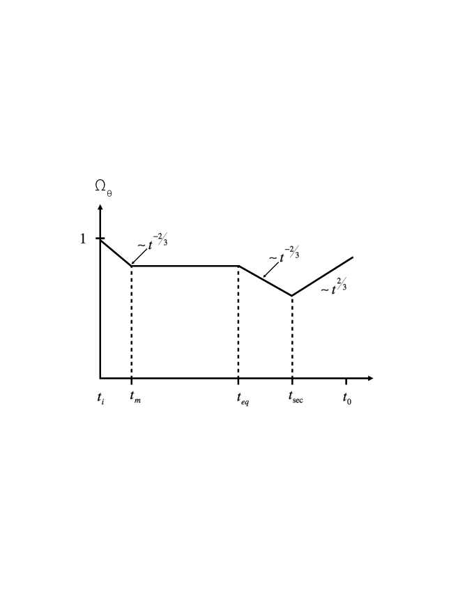
Figure 1: Sketch of the time evolution of the fractional contribution $\Omega_{\theta}$ of the $\theta$ field to energy density of the Universe. The horizontal axis is time, the vertical axis is the value of $\Omega_{\theta}$. The value of $\Omega_{\theta}$ initially decays from $t_{i}$ until $t_{m}$. Between $t_{m}$ and $t_{eq}$ we have exact tracking, i.e. $\Omega_{\theta}$ is constant. For $t>t_{eq}$ the value of $\Omega_{\theta}$ initially decreases until the timie $t_{sec}$ when the secular growth term for the electric field $E$ becomes important, after which $\Omega_{\theta}$ grows (for illustrative purposes we have chosen $G(t)$ such that the growth is proportional to the scale factor).

V Conclusions and Discussion

We have proposed a model involving a complex scalar field $\varphi$ that can give rise to both Dark Matter and Dark Energy. Dark Matter is provided by the radial oscillations of the field $\varphi$ about its symmetry breaking minimum, Dark Energy by the angular variable, which is a new axion. A key feature of our model is a coupling of the axion to the Pontryagin density of a non-abelian gauge field. The field $\varphi$ is introduced in analogy to the Peccei-Quinn scalar of QCD. The phase of $\varphi$ couples to the Pontryagin density of the gauge field. This provides a mechanism for very slow rolling of the angular variable $\theta$, so that $\theta$ can yield Dark Energy. In turn, the dynamics of $\theta$, assisted by an additional axial chemical potential, induces secular growth of the electric component, $E$, of the gauge field. Once the secular growth term in $E$ starts to dominate over the usual term, the contribution of $\theta$ to the total energy density starts to grow. Thus, $\theta$ is a candidate for tracking quintessence.

In our model, the energy density, $\rho_{A}$, of the gauge field represents an extra contribution to Dark Matter. For sufficiently large values of the coefficient $\alpha$ one can ensure that $\rho_{A}$ is negligible at the present time. However, eventually $\rho_{A}$ will grow faster than the density of Dark Energy. Thus, our model predicts that the period of Dark Energy domination does not continue arbitrarily far into the future.

In our setup, the approximate equality of the energy densities in Dark Matter and Dark Energy has a natural explanation since the energy densities of the two components are proportional during most of the evolution of the universe (from $t_{m}$ until $t_{eq}$). For $t_{i}<t_{m}$ and for $t_{eq}<t_{sec}$ the contribution of $\theta$ decays relative to that of Dark Matter, whereas it increases after $t_{sec}$.We need $t_{sec}$ to lie in the interval $[t_{eq},t_{0}]$.

If $\theta$ is to be a viable candidate for Dark Energy, it has to be very weakly coupled to electromagnetism Carroll . This is why we need to introduce a new gauge field which $\varphi$ couples to. Since, in our setup, Dark Matter and Dark Energy belong to the same sector, our model predicts that Dark Matter has negligible interactions with regular matter. Direct detection of Dark Matter in accelerator experiments or in underground laboratories would rule out our scenario.

In our model, Dark Matter is coupled to Dark Energy. This coupling gives rise to interesting predictions on observations, as was studied in toy models of the two dark sectors in Abdalla and references therein. Work on this topic is in progress.

As for the QCD axion, we have to cope with a potential domain wall problem DW . If the values of the potential at field values $\theta=0$ and $\theta=\pi$ are exactly the same, then if the $\varphi$ field begins in thermal equilibrium and undergoes a symmetry breaking phase transition a network of domain walls will inevitably form by causality Kibble . This network would acquire a “scaling solution” (the network looks the same at all times when lengths are scaled to the Hubble radius $t$) and would persist to the present time. A single domain wall in our Hubble radius would overclose the universe if the symmetry breaking scale is above roughly $1{\rm TeV}$; (see e.g. CSrevs for reviews of the cosmology of topological defects). We can avoid this domain wall problem in the same way it is avoided for QCD axions. For example, we could slightly lift the potential to make $\theta=0$ the unique vacuum state. We could also assume that an early period of cosmological inflation provides the causal connections on super-Hubble scales which leads $\varphi$ to fall into the same vacuum state everywhere in the observable part of the Universe.

There has been other recent work connecting the two dark sectors in the context of QCD-like theories; see, e.g., Stephon1 (which is based on Stephon2 ).

Appendix A: Origin of the Axial Chemical Potential

In this section we present a possible scenario for the origin of the axial chemical potential $\mu_{5}$. Let us consider a second scalar field $\chi$ coupling to $E\cdot B$, in analogy to the angular field variable $\theta$, i.e., with a coupling given by (5). We take $\chi$ to have vanishing mass dimension, as assumed in (5). We can introduce a scalar field ${\tilde{\chi}}$ with the usual mass dimension $1$ by setting

$${\tilde{\chi}}\,\equiv\,\chi_{0}\chi\,,$$ (66)

where $\chi_{0}$ is some mass scale.

Let us assume that ${\tilde{\chi}}$ has an exponential potential of the form

$$V_{{\tilde{\chi}}}\,=\,V_{0}\bigl{[}e^{-{\tilde{\chi}}/\chi_{0}}-1\bigr{]}\,,$$ (67)

where the constant $V_{0}$ has mass dimension four. We also assume that ${\tilde{\chi}}$ couples to some heat bath. This induces a correction to the effective potential whose leading term is (see e.g. Dolan and the review in RMP )

$$\delta V\,=\,\frac{1}{2}T^{2}{\tilde{\chi}}^{2}\,.$$ (68)

If we assume that ${\tilde{\chi}}$ tracks the minimum of the effective potential we find that

$$\chi\,\sim\,\frac{V_{0}}{\chi_{0}^{2}}\bigl{(}\frac{T_{eq}}{T}\bigr{)}^{2}T_{eq}^{-2}\,,$$ (69)

for ${\tilde{\chi}}\ll\chi_{0}$, which leads to

$${\do{\chi}}\,\sim\frac{4}{3}\frac{V_{0}}{\chi_{0}^{2}}\frac{1}{t_{eq}}T_{eq}^{-2}\,,$$ (70)

for $t<t_{eq}$, and

$${\do{\chi}}\,\sim\frac{4}{3}\frac{V_{0}}{\chi_{0}^{2}}\frac{1}{t_{eq}}\bigl{(}\frac{t}{t_{eq}}\bigr{)}^{1/3}T_{eq}^{-2}\,,$$ (71)

for $t>t_{eq}$. Making use of the Friedmann equation to express the time $t_{eq}$ in terms of the energy density $T_{eq}^{4}$ at that time, we find that

$${\dot{\chi}}\,\sim\,\frac{V_{0}}{\chi_{0}^{2}m_{pl}}\,.$$ (72)

The fact that there is a factor of $m_{pl}$ (= Planck mass) in the denominator of (72) makes it possible to obtain a small value of ${\dot{\chi}}$, which leads to a small value of the axial chemical potential $\mu_{5}$, as required by the criterion (34). It does take some tuning of $V_{0}$ and $\chi_{0}$ to obtain a value of $\mu_{5}$ which lies exactly in the range given by (34).

Appendix B: Possible Resonance Effects

In our scenario, the radial field $r$ is oscillating. It is coupled to the angular variable $\theta$ via the nonlinear terms in the equations of motion. We must hence worry about possible resonance effects like the parametric instability by which the oscillations of the inflaton field at the end of the period of inflation induce exponential growth of fields coupled to the inflaton TB ; DK (see also RRevs for recent review articles).

To study the possible resonant excitation of $\theta$ due to the oscillations of $r$ we consider the equation of motion for fluctuations of $\theta$ about the background value $\theta_{0}$ considered in the main text:

$$\theta\,=\,\theta_{0}+\theta_{1}\,.$$ (73)

In the small amplitude limit for the fluctuation $\theta_{1}$ we have

$${\ddot{\theta}_{1}}+3H{\dot{\theta}_{1}}+\frac{{\dot{r}}}{R_{0}}{\dot{\theta}_{1}}\,=\,0\,.$$ (74)

This is in fact a first order differential equation for $\chi\equiv{\dot{\theta}_{1}}$ which has the solution

$${\rm ln}\bigl{(}\frac{\chi}{\chi_{i}}\bigr{)}\,=\,-3{\rm ln}\frac{t}{t_{i}}-\frac{2}{R_{0}}\int_{t_{i}}^{t}dt^{\prime}{\dot{r}}(t^{\prime})\,,$$ (75)

where $t_{i}$ is the initial time and $\chi_{i}$ is the value of $\chi$ at that time. Since the integrand on the right hand side of the above equation is oscillating, there is clearly no resonant growth.

Above, we have shown that oscillations of the $r$ field does not induce a parametric resonance instability for $\theta$ fluctuations. However, to ensure that our estimate of the dark matter density from the $r$ field is correct, we must also ensure that the perturbative decay of $r$ is not too efficient. For an interaction Lagrangian describing the decay of a canonically normalized field $r$ into another canonically normalized field $\chi$

$${\cal L}_{int}\,=\,-g\sigma r\chi^{2}\,,$$ (76)

the perturbative decay $\Gamma$ rate is given by

$$\Gamma\,=\,\frac{g^{2}\sigma^{2}}{8\pi m}\,,$$ (77)

where $m$ is the mass of the oscillating field. In our case $\chi=R_{0}\theta_{1}$, where $\theta_{1}$ is the fluctuation of $\theta$ about the slow-roll solution $\theta$ given by (15). Expanding the Lagrangian (II) to leading quadrtic order in $\theta_{1}$ we can read off what corresponds to $g\sigma$ in the general case. The mass of $r$ can be read off of the same Lagrangian. Then, one finds that in our case the ratio

$$\frac{\Gamma}{H}\,\sim\,\mu^{5/3}\lambda^{-1/2}\alpha^{2/3}\bigl{(}\frac{E\cdot B}{R_{0}^{4}}\bigr{)}^{2/3}\,,$$ (78)

and we can see that it is not hard to choose parameters and initial conditions on the energy density in the new gauge field such that already at the time $t_{m}$

$$\frac{\Gamma(t_{m})}{H(t_{m})}\,\ll\,1\,,$$ (79)

and that hence perturbative decay is negligible. Hence, our dark matter candidate does not decay efficiently into dark energy.

References

- (1) P. A. R. Ade et al. [Planck Collaboration], “Planck 2015 results. XIII. Cosmological parameters,” arXiv:1502.01589 [astro-ph.CO].
-
(2)
J. C. Kapteyn, “First attempt at a theory of the arrangement and motion of the sidereal system”, Astrophysical Journal 55, 302 – 327 (1922)
F. Zwicky, “Die Rotverschiebung von extragalaktischen Nebeln”. Helvetica Physica Acta 6, 110 – 127 (1933) - (3) V. C. Rubin and W. K. Ford, Jr., “Rotation of the Andromeda Nebula from a Spectroscopic Survey of Emission Regions,” Astrophys. J. 159, 379 (1970). doi:10.1086/150317
- (4) R. H. Brandenberger, “Lectures on the theory of cosmological perturbations,” Lect. Notes Phys. 646, 127 (2004) [hep-th/0306071].
- (5) S. Perlmutter et al. [Supernova Cosmology Project Collaboration], “Discovery of a supernova explosion at half the age of the Universe and its cosmological implications,” Nature 391, 51 (1998) doi:10.1038/34124 [astro-ph/9712212].
- (6) A. G. Riess et al. [Supernova Search Team Collaboration], “Observational evidence from supernovae for an accelerating universe and a cosmological constant,” Astron. J. 116, 1009 (1998) doi:10.1086/300499 [astro-ph/9805201].
-
(7)
M. Li, X. D. Li, S. Wang and Y. Wang,