Topological Gapless Phases in Non-Symmorphic Antiferromagnets

Abstract

Topologically protected fermionic quasiparticles occur in metals with band degeneracy as a consequence of band structure topology. Here we unveil topological semimetal and metal phases in a variety of non-symmorphic collinear antiferromagnets with glide reflection symmetry, a combination of mirror and half-lattice translation. We find gapless phases with Dirac points having multiple symmetry-protection as well as electronic structures with triple and quadruple band-crossing points. Glide semimetal is shown to be converted into a topological phase with non-trivial $\mathbb{Z}_{2}$ topological charges at the Dirac points due to inversion and time-inversion symmetry combination. More striking is the emergence of a hidden non-unitary relation between the states in the glide sectors that provide a general mechanism to get multiple band touching points. The split Fermi points uncover a $\mathbb{Z}_{2}$ protection that drives the changeover of the multiple-degenerate gapless phase into a topological metal built from their connection through distinct Fermi lines. Besides a new perspective of ordered states in complex materials, our findings indicate that novel topological gapless phases and edge states may occur in a wide class of magnetic systems.

I Introduction

Topological materials have become the focus of intense research in the last years Hasan2010 ; Qi2011 ; Chiu2016 ; Weng2015a not only for the perspective of new physical phenomena with potential technological applications, but also for being a test bed for fundamental concepts of physics theories. Along this line, recent efforts led to the theoretical prediction Kane2005 ; Bernevig2006 ; Moore2007 ; Fu2007 and experimental realization Konig2007 ; Hsieh2008 ; Xia2009a of topological insulators in materials with strong spin-orbit coupling (SOC). One of the hallmarks of TIs is the existence of protected gapless edge states, which are due to a non-trivial topology of the bulk band structure. Such manifestation of topological order however is not limited to insulators as electronic structures with gapless topological modes have been predicted Volovik2003 ; Volovik2007 ; Wan2011 ; Heikkila2011 ; Yang2011 ; Burkov2011 ; Krempa2012 ; Xu2011 ; Halasz2012 and their relevance further boosted by the discovery of novel materials Weng2015b ; Huang2015 ; Xu2015a ; Lv2015a ; Lv2015b ; Xu2015b with non-trivial band crossing points in the momentum space and robust edge states.

Among various kinds of topological matter, correlated materials Imada1998 ; Tokura2000 with strong spin-orbital-charge entanglement Oles2012 ; Vojta2009 ; Brz2015 ; Brz16 , e.g. transition-metal oxides, represent a unique platform to explore topological effects combined to a large variety of intriguing collective properties emerging from electron-electron interaction, as superconductivity, magnetism, magnetoelectricity and Mott insulating phases. In these systems, complex magnetic orders generally arise from competing ferromagnetic (FM) and antiferromagnetic (AF) correlations with a frustrated localized-itinerant nature and a strong dependence on the orbital character of the transition metal $d$-shells. Magnetic patterns constructed by antiferromagnetically coupled zig-zag FM chains (Figs. 1(a),(b)) are one generic manifestation of such competing effects and often occur in the class of correlated materials as demonstrated in manganites Tokura2006 ; Munoz2001 ; Dong2015 , ruthenates Ortmann2013 ; Mathieu2005 ; Hossain2012 ; Mesa2012 , dichalcogenides Xia2009b ; Chen2009 ; Fobes2014 , iridates Ye2012 ; Choi2012 , nickelates Munoz1994 ; Alonso1999 ; Diaz2001 ; Zhou2005 , etc. A relevant mark of zig-zag patterns is the symmetry under non-symmorphic (NS) transformations that combine point group operations with translation that are a fraction of a Bravais lattice vector Bradley1972 . Recently, NS groups have been recognized as a new source of topological symmetry protection both in gapped Mong2010 ; Liu2014 ; Fang2015 ; Shiozaki2015 ; Dong2016 ; Wang2016 ; Varjas2015 ; Sahoo2015 ; Lu2016 ; Shiozaki2016a ; Kobayashi2016 ; Alexandradinata2016 ; Chang2016 ; Wang2016Nat and gapless Parameswaran2013 ; Watanabe2015a ; Young2015 ; Watanabe2016 ; Liang2016 ; Venderbos2016 ; Yang2016 ; Muechler2016 ; Zhan2016 ; Bzdusek2016 ; Wieder2016 ; Bradlyn2016 ; Chen2016 ; Wieder2016a ; Pixley2016 systems. Hence, given the wide range of physical phenomena in both topological and correlated materials, the identification of novel topological phases in the presence of non trivial orderings and their material realizations represent a fundamental challenge in the condensed matter area.

In this paper, we unveil topological semimetal (SM) and metal phases in a variety of non-symmorphic collinear antiferromagnets with glide reflection symmetry. The emergent topological gapless states can exhibit Dirac points (DPs) with multiple symmetry-protection as well as three- and four-fold degenerate DPs. Besides non-symmorphic symmetry protection, we demonstrate that combination of inversion and time or particle-hole symmetry can lead to non-trivial $\mathbb{Z}_{2}$ topological charges at the DPs, thus building up a robust topological gapless phase. More striking is the occurrence of a hidden symmetry-like relation between the states in the two glide sectors that provide a general mechanism to stick DPs or generate multiple band touching points in the glide plane (GP). We show how the splitting of the multiple degenerate Fermi points (FPs) drives the transition into a topological metal. Due to a $\mathbb{Z}_{2}$ protection of the DPs in the glide plane, a topological metal arises with multiple Fermi pockets resulting from the Fermi lines connecting the DPs themselves.

The paper is organized as follows. In Sec. II we present the model Hamiltonian employed to describe the zigzag antiferromagnets and the related symmetries. Sec. III is devoted to discuss the phase diagram and the most relevant topological phases emerging among the obtained electronic structures. In the Sec. IV, we provide the concluding remarks. The various technical details including some representative cases of energy spectra for the zig-zag antiferromagnetic phases are given in the Appendices A-G.

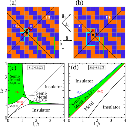
Figure 1: (Color online) Zig-zag spin patterns with (a) length $L_{z}=2$ ($z2$) and (b) $L_{z}=3$ ($z3$). Orange and blue squares indicate spin-up and spin-down orientation. The unit cell is marked by a thick blue frame while $\hat{a}_{1,2}$ are the translation directions. The square unit cells are marked with green frames. Dashed lines indicate the normal mirror planes $m_{1}$ and $m_{2}$, with $m_{2}$ being related to the the gliding symmetry. The glide transformations is sketched via the red dots and arrows; the dot is subjected to the reflection $m_{2}$ then it is translated by a vector $\vec{t}$ parallel to the mirror plane $m_{2}$. For $z2$ these two steps separately do not reproduce the original lattice. The black dots are the inversion centers. Phase diagrams for (c) $z2$ at $3/4$ filling and (d) $z3$ at half filling. Topological semimetal phases are marked with color (green area) and the position of Dirac points in the Brillouin zone is reported in parenthesis. Red and blue lines in (c) and (d) indicate configurations where the Dirac points are in high symmetry positions.

II Model and symmetries

We consider an effective orbital-directional double-exchange model describing itinerant electrons (e.g. t_2g or $p$ bands) in the presence of an anisotropic SOC, as due to tetragonal crystal field splitting, and Hund coupled to localized spin moments forming zig-zag pattern with characteristic length $L_{z}\geq 2$. The model Hamiltonian is given by

$${\cal H} = \sum_{i,\sigma}\sum_{{\alpha,\beta=a,b\atop{\hat{\gamma}}={\hat{a},\hat{b}}}}t_{\gamma,\alpha\beta}\left(d_{i,\alpha\sigma}^{\dagger}d_{i+\hat{\gamma},\beta\sigma}+h.c.\right)$$

$$- J_{H}\!\!\!\sum_{i,\alpha=a,b}\!\!s^{z}_{i\alpha}\cdot S^{z}_{i}+\lambda\sum_{i}S_{i}^{z}l_{i}^{z}\,,$$

where $d^{\dagger}_{i,\alpha\sigma}$ is the electron creation operator at the site $i$ with spin $\sigma$ for the orbital $\alpha$, $(a,b,c)$ are the $(yz,xz,xy)$ orbitals which are perpendicular to the corresponding bond direction, with $\hat{a}$, $\hat{b}$, and $\hat{c}$ being the unit vectors along the lattice symmetry directions. $\alpha$, ${\bf s}_{i\alpha}\!=\!d_{i,\mu,\alpha}^{\dagger}\sigma^{z}_{\!\alpha,\beta}d_{i,\mu,\beta}$ and $S^{z}_{i}=\pm 1$ denote the spins for the $d_{xz/yz}$ and $d_{xy}$ orbitals, respectively. $J_{H}$ stands for the Hund coupling, while $\lambda$ is the SOC for the projected subspace of $(a,b)$ orbitals, with $l_{i}^{z}=i\left(d_{i,a,\sigma}^{\dagger}d_{i,b,\sigma}-d_{i,b,\sigma}^{\dagger}d_{i,a,\sigma}\right)$ the $z$-component of the local angular momentum. $t_{\hat{\gamma},\alpha\beta}$ is the nearest-neighbor hopping amplitude between $\alpha$ and $\beta$ for the bond along the $\hat{\gamma}$ direction. We assume cubic symmetric hopping amplitudes, i.e., $t_{\hat{a},bb}=t_{\hat{b},aa}=-t$ with $t$ as energy scale unit and $t_{\hat{\gamma},ab}=0$. The AF states are collinear and the spin $z$-projection is a conserved quantity due to the anisotropic SOC. The exact matrix forms of the $k$-space Hamiltonians ${\cal H}_{\vec{k}}$ for $L_{z}=2,3$ are given in the Appendices A and B.8.

While the Hamiltonian resembles the double-exchange model widely applied in the context of manganese oxides, it contains extra microscopic ingredients as orbital directionality and spin-orbit coupling that contribute to give unique features in the phase diagram and the electronic spectra. For instance, zig-zag states have been demonstrated to be among the energetically most favorable configurations in a large range of doping concentration for the case of $d_{xz/yz}$ bands Brzezicki2015 and to be relevant for providing novel scenarios and mechanisms to understand the occurrence of zig-zag spin patterns with length $L_{z}=2$ (i.e. $z2$) in Mn doped bilayer ruthenates Sr₃Ru₂O₇ and in other similar hybrid oxides. Furthermore, it can be considered as an effective low energy description of correlated $t_{2g}$ electrons in transition metal oxides with orbital selective localized and itinerant bands such as to yield a double exchange model. Indeed, as a consequence of the atomic Coulomb interaction in multi-orbital systems, an orbital selective Mott transition can occur and lead to electronic localization in a subgroup of the $t_{2g}$ bands. Such reduction from a multi-orbital correlated system to an effective double-exchange has been generally addressed and demonstrated to be applicable in the context of orbital-selective-Mott physics orbsel-PRL05 ; orbsel-PRL14 .

The symmetry properties of the model Hamiltonian include transformations that act on the internal (e.g. spin, orbital, charge) and spatial degrees of freedom, or combine them, including the possibility of having groups with non-primitive lattice vector translational (e.g. non-symmorphic groups). Concerning the internal symmetries, the model exhibits only time reversal invariance, ${\cal T}$ with ${\cal T}{{}^{2}}=1$ and ${\cal T}^{\dagger}{\cal H}_{\vec{k}}{\cal T}={\cal H}^{T}_{-\vec{k}}$.

For the spatial symmetries, electrons move on a square lattice and within a magnetic pattern due to a broken symmetry ground-state. The model Hamiltonian can exhibit invariance under a reflection plane $m_{1}$ and has inversion centers (see Figs. 1(a)-(b)) associated to the reflection and inversion operators, $\cal R$ and $\cal I$ respectively. Then, in two dimensions it is known that there are other relevant symmetry operations belonging to the non-symmorphic groups which include screw axis, glide mirror lines, and glide mirror planes in conjunction with the translation Bradley1972 . The zig-zag antiferromagnet (AFM) is invariant under a NS glide transformation ${\cal R}^{t}$ which is constructed by the product of a reflection with respect to the $m_{2}$ plane and a translation $\vec{t}\equiv\vec{a}_{2}/2$ in the $\hat{a}_{2}$ direction along the zig-zag chain (Figs. 1(a)-(b)). Due to the multi-orbital character of the model Hamiltonian, both ${\cal R}$ and ${\cal R}^{t}$ include spatial and orbital transformations. Indeed, the mirror reflections interchange the $\hat{a}$ and $\hat{b}$ lattice directions and consequently the orbitals, see Appendix B.2. ${\cal R}^{t}$ is also intrinsically $k$-dependent as it is not possible to find a unit cell that maps onto itself under the glide transformation. By a proper choice of the unit cell or a suitable $k$-dependent transformation of ${\cal H}_{\vec{k}}$, as thoroughly discussed and demonstrated in the Appendix B.7, one can show that the glide operator depends only on $k_{2}$ as ${\cal R}_{k_{2}}^{t}$. We select a basis that makes ${\cal R}_{k_{2}}^{t}$ to have eigenvalues $g_{\pm}=\pm 1$ while the eigenvectors carry the $k_{2}$-dependence. As expected from the half-lattice translation of NS symmetry, the glide eigenstates have a doubled period in the momentum space. It is worth pointing out that ordinary reflection ${\cal R}$ is also $k$-dependent for the present choice of the unit cell (see Fig. 4 in the Appendix for a detailed view and description of the unit cell) but it can be made completely $k$-independent by a suitable gauge transformation (as shown in Appendix B.6) without affecting the periodicity of ${\cal H}_{\vec{k}}$.

At half filling, the model Hamiltonian exhibits a non-symmorphic like chirality operator ${\cal S}_{k_{1}}$ (and then also a particle-hole ${\cal C}_{k_{1}}$), as it carries an intrinsic $k_{1}$-dependence Shiozaki2016a and acts to yield ${\cal S}_{k_{1}}^{\dagger}{\cal H}_{\vec{k}}{\cal S}_{k_{1}}=-{\cal H}_{\vec{k}}$. The details of the structure and the properties are explicitly reported and discussed in the Appendix B.1. As for the chirality, also the inversion ${\cal I}$ symmetry carries an intrinsic $k$-dependence which is tightly linked to the structure of the zig-zag magnetic pattern and the non-symmorphic glide symmetry. A peculiar feature of the symmetry properties is that their $k$-dependence can be removed only by allowing a period elongation for the eigenstate of the Hamiltonian in the Brillouin zone, as explicitly demonstrated in the Appendix B.5. The reason for that is ascribable to the lack of a unit cell that would map onto itself under the action of these operators. Concerning the relations between the symmetry operators, all spatial symmetries commute between each other and with time reversal while reflection $\cal R$ commutes also with chirality. Glide and inversion commutes/anticommutes with chirality (thus also $\cal C$) for odd/even $L_{z}$, see Appendices B.3. Combined spatial-non-spatial symmetries can also be relevant for the character of the electronic structure and thus for completeness their properties are explicitly reported in the Appendix B.4.

Finally, concerning the symmetry aspects of the model Hamiltonian, we also mention that there occur special symmetries that act only in the parameter space. Indeed, one can identify reflections in the parameter space of the Hund and spin-orbit couplings $(J_{H},\lambda)$ which can be expressed by an SU($2$) algebra through their generators $\cal X$ and $\cal Y$. The explicit form of the parameters space reflection symmetry is reported in the Appendix B.9.

III Results

Concerning the electronic behavior of zig-zag AFM, our focus is on $z2$ and $z3$ magnetic patterns which are those more relevant for the materials perspective as discussed in the introduction. A generic feature of the electronic phase diagram is that both SOC and Hund interaction are able to yield an insulating state that can be generally ascribed to the formation of almost disconnected orbital molecules developing within the zig-zag path due to the orbital directionality of the $d_{xz/yz}$ bands Brzezicki2015 . Then, the relative ratio of the SOC and Hund coupling can drive a series of (semi)metal-insulator transitions where non-trivial gapless phases are robust to variation of the microscopic parameters or occur in between the insulating states as demonstrated for two representative electron densities in Figs. 1 (c),(d). Another relevant aspect of the electronic phase diagram is that the semimetal states can have Dirac points in the normal mirror, in the glide planes, or in a generic position of the Brillouin zone, thus indicating that both non-spatial and spatial symmetries can be crucial in protecting the Fermi surface. Moreover, along the diagonal of the phase diagram a semimetal phase is obtained with Dirac points always lying in one of the glide plane, i.e. at $k_{1}=0$. Such finding is specific of the model Hamiltonian and is a consequence of a symmetry in the parameter space that interchanges $J_{H}$ with $\lambda$ or $J_{H}$ with $-\lambda$ in ${\cal H}_{\vec{k}}$, as also described in more details in Appendix B.9.

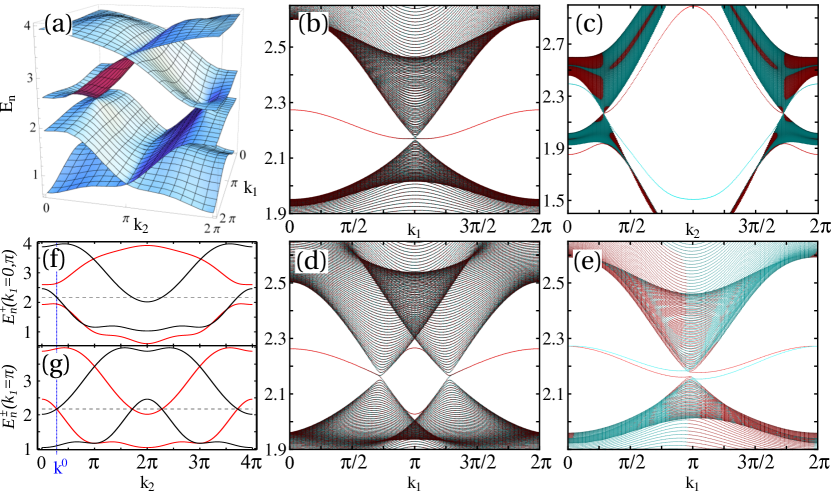
Figure 2: Electronic spectra for $z2$ AF at $3/4$ filling. (a) Bulk energy spectrum above zero energy. (b)-(e) one-dimensional spectra and edge states for a slab geometry with open boundary. Spectra for a slab configuration with open boundary in the (b) $\hat{a}_{1}$ and (c) $\hat{a}_{2}$ directions, with $k_{2}$ and $k_{1}$ being the momentum parallel to the edge, respectively. Electronic spectra with (d) open boundary along $\hat{a}_{2}$, broken glide and reflection symmetries with inversion invariance, and (e) with only broken time-reversal. (f) $g_{+}$ glide symmetric bands at $k_{1}=0$ (red) and $k_{1}=\pi$ (black) as functions of $k_{2}$. (g) Band structure in the glide plane at $k_{1}=\pi$, with glide eigenvalues $+1$ (red) and $-1$ (black). Dashed line sets the Fermi level. Color map of the spectra in (b)-(e) with high (low) brightness indicates a large (small) probability of the electronic states to be localized on the left (red) or right (blue) boundary.

For the topological properties of the resulting electronic phases, we start discussing the insulating phases. According to the character of the internal symmetries of the model Hamiltonian (i.e. ${\cal T}^{2}=1$) the system is in the AI class of the ten-fold Altland-Zirnbauer classification table Altland . For this case, in two-dimensions the fully gapped states cannot have any topological protection due to the non-spatial symmetries. On the other hand, for the gapless phases (Fermi lines or points) non-trivial topological invariants are allowed in the AI class.

The presence of symmetries that act nonlocally in position space can in principle expand the possibilities of having non-trivial topological properties both for the insulating and the gapless phases. For the AI class it turns out that the insulating phase in two-dimension are always trivial both in the presence of normal mirror symmetry Sch14 or non-symmorphic transformations Shiozaki2016a . Hence, the main aim is to investigate the eventual topological character of the gapless states.

We start by considering the $z2$ AFM and we focus on the DPs in the glide plane because our primary interest is to address the role of the non-symmorphic glide symmetry. We will see that not only the glide, but also the inversion, and combination of inversion with time-reversal combination are relevant symmetries for protecting the semimetal phase (Fig.2).

To set the stage, let us start discussing the band structure in the GP at $k_{1}=\pi$ (Fig. 2(g)) which is representative of the electronic phase at large spin-orbit coupling in the diagram of Fig. 1(c) . Since the glide ${\cal R}_{k_{2}}^{t}$ commutes with ${\cal H}_{\vec{k}}$, the electronic states can be labeled by $g_{\pm}$ glide eigenvalues. The DPs occur at the crossing of the bands with opposite $g$ and they are then protected by the glide symmetry. Furthermore, we find that in the one-dimensional (1D) cuts at any given $k_{2}$ the system has an inversion topological number $\mathbb{Z}^{\geq}$ Ber14 , with the inversion symmetry expressed by ${\cal R}_{k_{2}}^{t}$. $\mathbb{Z}^{\geq}$ is defined as the difference of the number of occupied states with a chosen inversion eigenvalue at the two inversion invariant points, $k_{1}=0$ and $k_{1}=\pi$. Taking the spectra in the $g_{+}$ glide sector at $k_{1}=\{0,\pi\}$, one can immediately deduce that $\mathbb{Z}^{\geq}$ changes sign at the position of the DPS, i.e. $k^{0}$ and $2\pi-k^{0}$. The inversion symmetry protection of the DPs explains the presence of a third edge state close to the zone boundary in Fig. 2(c). In the absence of glide symmetry, $\mathbb{Z}^{\geq}$ is meaningful only in the two high-symmetry cuts of the BZ, i.e. $k_{2}=\{0,\pi\}$, and it is non-trivial at $k_{2}=0$ but trivial at $k_{2}=\pi$, so there must be gap closings between these two 1D cuts (Fig. 1(f)). Finally, the $z2$ state exhibits also a symmetry protection arising from the combination of ${\cal I}$ and $\cal{T}$. Their product yields a conjugation operator, ${\cal K}_{\vec{k}}\equiv{\cal I}_{\vec{k}}{\cal T}$, since ${\cal K}$ transforms ${\cal H}_{\vec{k}}$ into ${\cal H}^{T}_{\vec{k}}$. If ${\cal K}_{\vec{k}}{\cal K}_{\vec{k}}^{\star}\equiv 1$ (which is satisfied for any $L_{z}$) then ${\cal H}$ can be made purely real in the eigenbasis of ${\cal K}_{\vec{k}}$ (as demonstrated explicitly in the Appendix C). Indeed, close to the DPs, the low energy Hamiltonian has a form $H_{\delta\vec{k}}=\delta k_{1}A+\delta k_{2}B$ with $A$ and $B$ being $2\times 2$ real matrices and $\delta\vec{k}$ the deviation with respect to the DP. The charge can be then calculated as a $\mathbb{Z}_{2}^{(1)}$ mod-$2$ winding number (see Appendix G), and it takes values $\pm 1$ at the two DPs. Though the time-inversion operator ${\cal K}$ is explicitly dependent on the momentum, in the low-energy description the result is consistent with the general expectation Zha2016 of having a non-trivial $\mathbb{Z}_{2}$ topological invariant at the DPs by combination of time and inversion symmetry. Hence, the resulting electronic spectra for the $z2$ phase in Figs. 2 (b)-(e) provide evidence of a peculiar topological resilience of DPs and edge modes, being robust to different types of symmetry breaking configurations.

Concerning the lowering symmetry perturbations, we point out that breaking of glide in such a way that inversion is not preserved opens a gap and the system becomes topologically trivial, consistently with the expectations from the classification table for the AI class in the presence of a mirror reflection Sch14 . Otherwise, breaking of the reflection or time only removes the $\mathbb{Z}_{2}$ protection but leaves the glide symmetry so that the DPs are still preserved. In Fig. 2(e) a representative case of time-reversal violation is also considered. Due to a termination dependent orbital polarization, non-degenerate chiral states emerge at the edge and, remarkably, the system allows for non-vanishing charge and orbital currents at the boundary.

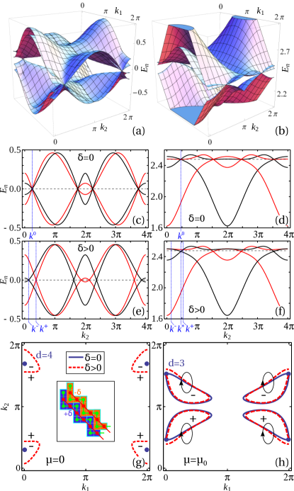
Figure 3: Multiple FPs in $z3$ antiferromagnet. (a) bands with chiral four-fold DPs at half filling ($\mu=0$), (b) bands with three-fold Fermi points at higher filling ($\mu=\mu_{0}$). (c), (d) the same bands in the glide plane $k=0$ with color indicating the glide eigenvalue $+1$ (red) and $-1$ (black). Dashed line is the Fermi level $\mu$. (e), (f) as in (c) and (d) plus a symmetry conserving long-range hopping $\delta$. (g), (h) FSs containing multiple FPs at $\delta=0$ (blue) and $\delta>0$ (red dashed). Multiple band crossing points are marked with dots and their degeneracy is indicated. The inset of (g) shows a schematic view of the hopping $\delta$. The signs in (g) indicate the band parity, $+1$ inside the Fermi pockets and $-1$ outside. The signs in (h) are those due the AI winding numbers of the Fermi lines. The integration contours are indicated by ellipses.

Let us consider the $z3$ AFM for two representative electron densities; at half-filling and away from it, at $\mu=\mu_{0}$. Firstly, we would like to focus on the consequence of the glide symmetry on the electronic spectra by investigating the origin of the observed multiple band touchings in the glide plane, as depicted in the Figs. 3(a),(b). Indeed, the gapless phases in the GPs for $z3$ AFM can exhibit quadruple and triple band touchings at half-filling and away from it, respectively (Figs. 3(a),(b)). As we will discuss more extensively later on, a prerequisite for having multiple Fermi points is to get DPs that are topologically protected in the glide plane. Furthermore, we find that the DPs can get glued and that the multiplicity of the FPs is not accidental but it also arises as a consequence of the glide symmetry. Their origin the GPs is due to a hidden non-unitary relation that leaves invariant the determinant of the glide-block Hamiltonian. One can demonstrate (see Appendix E) that for the Hamiltonian projected in the GP the two blocks are related by a $2\pi$ shift, i.e., $H_{0,k_{2}}^{+}=H_{0,k_{2}+2\pi}^{-}$. However, while the spectrum of $H_{0,k_{2}}^{+}$ is $4\pi$-periodic, due to the non-primitive half-lattice translation of the glide symmetry, its determinant has a $2\pi$-periodicity, $\rm{det}(H_{0,k_{2}}^{+}-\mu)\equiv\rm{det}(H_{0,k_{2}+2\pi}^{+}-\mu)$. It is important noticing that such property of the determinant does not depend on the chiral symmetry of the spectrum, because it manifests both at $\mu=0$ and $\mu=\mu_{0}=\sqrt{2+J_{H}^{2}+\lambda^{2}}$, respectively. We argue that such feature is remnant of the original periodicity of the full Hamiltonian and it implies that a $\mu$ eigenvalue of $H_{0,k_{2}}^{+}$ must be $2\pi$ periodic. Then, ($i$) the $2\pi$-shift relation of the glide symmetric blocks and ($ii$) the $2\pi$-periodic determinant combine to glue together DPs from different glide-blocks at two specific energy levels, $\mu=0,\mu_{0}$. We point out that while such property has similarity with the congruence, it is not exactly equivalent. Indeed, only a hermitian congruence is found between the blocks $H^{+}_{0,k_{2}}$ and $H^{+}_{0,k_{2}+2\pi}$, thus meaning that in a given basis these blocks differ only by a scaling of the rows and columns entries Rem . The anomalous periodicity of the determinant can be constructed explicitly, as demonstrated in the Appendix F, through a non-unitary chiral-like operator $\Sigma_{k_{2}}\equiv h_{k_{2}}^{-1}\bar{H}{}_{k_{2}}$ where $\bar{H}{}_{k_{2}}$ is the $2\pi$ periodic part of $H_{0,k_{2}}^{+}$ and $h_{k_{2}}$ is the part with $4\pi$ period ($h_{k_{2}+2\pi}\equiv-h_{k_{2}}$). The proof relies on the fact that eigenvalues of $\Sigma_{k_{2}}$ are symmetric around zero and on the Silvester property of determinants, i.e., $\rm{det}(1+AB)\equiv\rm{det}(1+BA)$. The emergence of a non-unitary relation that leaves the determinant invariant represents a novel mechanism for the search and generation of multiple band touching points in the presence of NS symmetries.

When breaking the conditions for the determinant invariance in the glide sectors, the DPs split into simple DPs. To show this behavior we add a symmetry conserving second and third nearest-neighbors hopping ($\delta$) in order to remove only the DPs degeneracy (Figs. 3(e),(f)). Such removal is concomitant with a transition from semimetal to metal whose Fermi surface (FS) is topological protected and has a structure which is strongly tied to the presence of topological non-trivial DPs in the glide plane. At $\mu=0$ and finite $\delta$ the FS has a topological character which arises from the glide symmetry and the induced non-symmorphic nature of the chiral transformation. Indeed, by combining the chiral and the conjugation symmetries we find a $k$-dpendent anticonjugation operator ${\cal A}_{\vec{k}}={\cal S}_{k_{1}}{\cal K}_{\vec{k}}$, which act to give a minus complex conjugate of ${\cal H}_{\vec{k}}$ (see Appendix D). One can show that ${\cal A}_{\vec{k}}{\cal A}_{\vec{k}}^{\star}\equiv 1$ for any odd $L_{z}$ and can be also rearranged as a product of the $k$-dependent inversion and particle-hole symmetry operators. We point out that due to its $k$-dependence, such symmetry is not explicitly included in the topological classification of a 1D FS by combination of particle-hole and inversion Zha2016 . Taking into account the structure of the ${\cal A}$ operator, one can construct a $\mathbb{Z}_{2}$ invariant by putting the Hamiltonian in the antisymmetric form using the eigenbasis of ${\cal A}_{\vec{k}}$ and calculating its Pfaffian (see Appendix D). The main result is that at the FS the Pfaffian changes sign and band inversion occurs (Fig. 3 (g)) thus the FS can be topologically protected. Apart from the whole FS, one can notice that in the GP, at $k_{1}=0$, the ${\cal A}$ operator is not $k$-dependent because the chirality depends only from $k_{1}$, and, thus, it also provides a protection for the DPs in both glide sectors. Then, if the metallic phase can be converted into a semimetal state by suitably tuning the microscopic parameters, the transition can only occur in the glide plane and the semimetal phase will exhibit multiple degenerate DPs, as it happens for instance at $\delta=0$. Such outcome can be generally expected for glide and chiral symmetric metallic phases in AI class which exhibit a topological protection in the full Brillouin zone and in one of the glide planes. Breaking of the glide symmetry opens a gap at the Fermi level everywhere in the Brillouin zone except that in the glide plane where DPs can be still protected by the conventional particle-hole and inversion combination Zha2016 as it is observed for the investigated electronic phases at half-filling. Hence, the emerging metallic phase is topologically protected and is marked by two Fermi pockets that are glued to the glide plane through the symmetry protected DPs. Away from half-filling, e.g. at $\mu=\mu_{0}$, the metallic phase is protected by the time symmetry as it exhibits a non trivial AI winding number $\mathbb{Z}$(see Appendix for the details of the calculation). In general we cannot have a semimetal phase and the triple band crossing coexists with a Fermi pocket (Fig. 3 (e)). The removal of the degeneracy by $\delta$ leads to an AI topological metal phase.

IV Conclusions

The realization of topological zig-zag AFMs and edge states has been so far focusing on insulating configurations Li2016 ; Brey2005 ; Du2015 . Our analysis demonstrates that the breakdown of the fully gapped phases in a multi-orbital zig-zag AFMs, due to the NS symmetry, can lead to topological gapless phases whose nature depends on the characteristic zig-zag length as well as on the intricate entanglement of non-symmorphic and internal or other spatial symmetries. The results demonstrate that, for a generic class of two-dimensional zig-zag AFMs with collinear magnetic order in the AI symmetry class, gapless phases are prone to exhibit a topological behavior. We find that the invariance of the determinants in the glide sectors is a novel mechanism, uniquely arising in NS systems, to generate multiple DPs and topological non-trivial gapless phases. Due to the observed $\mathbb{Z}_{2}$ protection of the Fermi points and the strong nesting of the topological metallic phase it is plausible to expect that the metallic phase can exhibit an anomalous magnetotransport response as well as a tendency to other electronic instabilities.

Concerning the materials perspective, there are many compounds exhibiting zig-zag magnetic patterns that involve $t_{2g}$ orbitals close to the Fermi level especially when considering transition metal oxides. In this framework, our results may find interesting application both in Mn doped ruthenates and dichalcogenides.

Acknowledgements W.B. acknowledges support by the European Horizon 2020 research and innovation programme under the Marie-Sklodowska-Curie grant agreement No. 655515 and by National Science Center (NCN) under Project No. 2012/04/A/ST3/00331.

Appendix A Stucture of the Hamiltonian for $L_{z}=2$ and $L_{z}=3$ zigzag patterns

The general form of the Hamiltonian in Eq. 1 (see main text) for a zigzag spin pattern can be obtained by analyzing the possible hopping processes for a given unit cell, as shown in Fig. 1 (see the main text). Its matrix representation for a given quasimomentum $\vec{k}$ and fixed spin polarization of the itinerant electrons, that is a good quantum number, can be conveniently written by a block matrix in the form

$${\cal H}_{\vec{k}}=\begin{pmatrix}{\bf H}_{\downarrow\downarrow}^{bb}&{\bf H}_{\downarrow\uparrow}^{bb}&{\bf H}_{\downarrow\downarrow}^{ba}&{\bf H}_{\downarrow\uparrow}^{ba}\\ {\bf H}_{\uparrow\downarrow}^{bb}&{\bf H}_{\uparrow\uparrow}^{bb}&{\bf H}_{\uparrow\downarrow}^{ba}&{\bf H}_{\uparrow\uparrow}^{ba}\\ {\bf H}_{\downarrow\downarrow}^{ab}&{\bf H}_{\downarrow\uparrow}^{ab}&{\bf H}_{\downarrow\downarrow}^{aa}&{\bf H}_{\downarrow\uparrow}^{aa}\\ {\bf H}_{\uparrow\downarrow}^{ab}&{\bf H}_{\uparrow\uparrow}^{ab}&{\bf H}_{\uparrow\downarrow}^{aa}&{\bf H}_{\uparrow\uparrow}^{aa}\end{pmatrix}.$$ (1)

Here, the blocks ${\bf H}_{\sigma\sigma^{\prime}}^{\alpha\beta}$($\sigma,\sigma^{\prime}=\uparrow,\downarrow$ and $\alpha,\alpha^{\prime}=a,b$) are of size $N_{\downarrow}=N_{\uparrow}=2L_{z}-2$, associated to the spin up and down domains within the unit cell (see Fig. 1). The indices $(\sigma\alpha)$ and $(\sigma^{{}^{\prime}}\beta)$ mean that the block describes hopping from the spin $\sigma$ to spin $\sigma^{\prime}$ domains and orbitals $\alpha$ and $\beta$, respectively. For $z2$ magnetic pattern the blocks for the electrons with spin up are given by the equations

$${\bf H}_{\downarrow\downarrow}^{bb} = \begin{pmatrix}J_{H}&-e^{-ik_{2}}t_{\hat{a}}^{bb}+t_{\hat{b}}^{bb}\\ -e^{ik_{2}}t_{\hat{a}}^{bb}+t_{\hat{b}}^{bb}&J_{H}\end{pmatrix},$$

$${\bf H}_{\uparrow\uparrow}^{bb} = \begin{pmatrix}-J_{H}&-e^{-ik_{2}}t_{\hat{a}}^{bb}+t_{\hat{b}}^{bb}\\ -e^{ik_{2}}t_{\hat{a}}^{bb}+t_{\hat{b}}^{bb}&-J_{H}\end{pmatrix},$$

$${\bf H}_{\downarrow\uparrow}^{bb} = \begin{pmatrix}0&e^{-ik_{2}}t_{\hat{b}}^{bb}-t_{\hat{a}}^{bb}\\ -e^{-ik_{1}}t_{\hat{a}}^{bb}+e^{i(k_{2}-k_{1})}t_{\hat{b}}^{bb}&0\end{pmatrix},$$

$${\bf H}_{\uparrow\downarrow}^{bb} = \left({\bf H}_{\downarrow\uparrow}^{bb}\right)^{\dagger},$$ (2)

for the $b$-orbital sector and

$${\bf H}_{\downarrow\downarrow}^{aa} = \begin{pmatrix}J_{H}&e^{-ik_{2}}t_{\hat{a}}^{aa}-t_{\hat{b}}^{aa}\\ e^{ik_{2}}t_{\hat{a}}^{aa}-t_{\hat{b}}^{aa}&J_{H}\end{pmatrix},$$

$${\bf H}_{\uparrow\uparrow}^{aa} = \begin{pmatrix}-J_{H}&e^{-ik_{2}}t_{\hat{a}}^{aa}-t_{\hat{b}}^{aa}\\ e^{ik_{2}}t_{\hat{a}}^{aa}-t_{\hat{b}}^{aa}&-J_{H}\end{pmatrix},$$

$${\bf H}_{\downarrow\uparrow}^{aa} = \begin{pmatrix}0&-e^{-ik_{2}}t_{\hat{b}}^{aa}+t_{\hat{a}}^{aa}\\ e^{-ik_{1}}t_{\hat{a}}^{aa}-e^{i(k_{2}-k_{1})}t_{\hat{b}}^{aa}&0\end{pmatrix},$$

$${\bf H}_{\uparrow\downarrow}^{aa} = \left({\bf H}_{\downarrow\uparrow}^{aa}\right)^{\dagger},$$ (3)

for the $a$-orbital sector. For the interorbital sector we have,

$${\bf H}_{\downarrow\downarrow}^{ba} = \begin{pmatrix}i\lambda&e^{-ik_{2}}t_{\hat{a}}^{ab}+t_{\hat{b}}^{ab}\\ -e^{ik_{2}}t_{\hat{a}}^{ab}-t_{\hat{b}}^{ab}&i\lambda\end{pmatrix},$$

$${\bf H}_{\uparrow\uparrow}^{ba} = \begin{pmatrix}-i\lambda&e^{-ik_{2}}t_{\hat{a}}^{ab}+t_{\hat{b}}^{ab}\\ -e^{ik_{2}}t_{\hat{a}}^{ab}-t_{\hat{b}}^{ab}&-i\lambda\end{pmatrix},$$

$${\bf H}_{\downarrow\uparrow}^{ba} = \begin{pmatrix}0&e^{-ik_{2}}t_{\hat{b}}^{ab}+t_{\hat{a}}^{ab}\\ -e^{-ik_{1}}t_{\hat{a}}^{ab}-e^{i(k_{2}-k_{1})}t_{\hat{b}}^{ab}&0\end{pmatrix},$$

$${\bf H}_{\uparrow\downarrow}^{ba} = \begin{pmatrix}0&e^{ik_{1}}t_{\hat{a}}^{ab}+e^{i(k_{1}-k_{2})}t_{\hat{b}}^{ab}\\ -e^{ik_{2}}t_{\hat{b}}^{ab}-t_{\hat{a}}^{ab}&0\end{pmatrix},$$ (4)

and the rest of blocks can be recovered from these as

$${\bf H}_{\sigma\sigma^{\prime}}^{ab}=\left({\bf H}_{\sigma^{\prime}\sigma}^{ba}\right)^{\dagger}.$$ (5)

We note that the spin sectors for the itinerant electrons are completely equivalent. It is immediate to verify that the Hamiltonian blocks for the opposite spin-sectors can be obtained by changing the sign of $J_{H}$ and $\lambda$. For zig-zag $z3$ the size of the spin domain is $N_{\downarrow}=4$ so that the blocks are twice larger. Then, we have

$${\bf H}_{\downarrow\downarrow}^{bb} = \begin{pmatrix}J_{H}&t_{\hat{b}}^{bb}&0&-e^{-ik_{2}}t_{\hat{a}}^{bb}\\ t_{\hat{b}}^{bb}&J_{H}&t_{\hat{b}}^{bb}&0\\ 0&t_{\hat{b}}^{bb}&J_{H}&-t_{\hat{a}}^{bb}\\ -e^{ik_{2}}t_{\hat{a}}^{bb}&0&-t_{\hat{a}}^{bb}&J_{H}\end{pmatrix},$$

$${\bf H}_{\uparrow\uparrow}^{bb} = \begin{pmatrix}-J_{H}&t_{\hat{b}}^{bb}&0&-e^{-ik_{2}}t_{\hat{a}}^{bb}\\ t_{\hat{b}}^{bb}&-J_{H}&t_{\hat{b}}^{bb}&0\\ 0&t_{\hat{b}}^{bb}&-J_{H}&-t_{\hat{a}}^{bb}\\ -e^{ik_{2}}t_{\hat{a}}^{bb}&0&-t_{\hat{a}}^{bb}&-J_{H}\end{pmatrix},$$

$${\bf H}_{\downarrow\uparrow}^{bb} = N_{\downarrow}\begin{pmatrix}0&-t_{\hat{a}}^{bb}&0&e^{-ik_{2}}t_{\hat{b}}^{bb}\\ -e^{-ik_{1}}t_{\hat{a}}^{bb}&0&-t_{\hat{a}}^{bb}&0\\ 0&-e^{-ik_{1}}t_{\hat{a}}^{bb}&0&e^{-ik_{1}}t_{\hat{b}}^{bb}\\ e^{i(k_{2}-k_{1})}t_{\hat{b}}^{bb}&0&t_{\hat{b}}^{bb}&0\end{pmatrix},$$

$${\bf H}_{\uparrow\downarrow}^{bb} = \left({\bf H}_{\downarrow\uparrow}^{bb}\right)^{\dagger},$$ (6)

for the $b$-orbital sector, and

$${\bf H}_{\downarrow\downarrow}^{aa} = \begin{pmatrix}J_{H}&-t_{\hat{b}}^{aa}&0&e^{-ik_{2}}t_{\hat{a}}^{aa}\\ -t_{\hat{b}}^{aa}&J_{H}&-t_{\hat{b}}^{aa}&0\\ 0&-t_{\hat{b}}^{aa}&J_{H}&t_{\hat{a}}^{aa}\\ e^{ik_{2}}t_{\hat{a}}^{aa}&0&t_{\hat{a}}^{aa}&J_{H}\end{pmatrix},$$

$${\bf H}_{\uparrow\uparrow}^{aa} = \begin{pmatrix}-J_{H}&-t_{\hat{b}}^{aa}&0&e^{-ik_{2}}t_{\hat{a}}^{aa}\\ -t_{\hat{b}}^{aa}&-J_{H}&-t_{\hat{b}}^{aa}&0\\ 0&-t_{\hat{b}}^{aa}&-J_{H}&t_{\hat{a}}^{aa}\\ e^{ik_{2}}t_{\hat{a}}^{aa}&0&t_{\hat{a}}^{aa}&-J_{H}\end{pmatrix},$$

$${\bf H}_{\downarrow\uparrow}^{aa} = \begin{pmatrix}0&t_{\hat{a}}^{aa}&0&-e^{-ik_{2}}t_{\hat{b}}^{aa}\\ e^{-ik_{1}}t_{\hat{a}}^{aa}&0&t_{\hat{a}}^{aa}&0\\ 0&e^{-ik_{1}}t_{\hat{a}}^{aa}&0&-e^{-ik_{1}}t_{\hat{b}}^{aa}\\ -e^{i(k_{2}-k_{1})}t_{\hat{b}}^{aa}&0&-t_{\hat{b}}^{aa}&0\end{pmatrix},$$

$${\bf H}_{\uparrow\downarrow}^{aa} = \left({\bf H}_{\downarrow\uparrow}^{aa}\right)^{\dagger},$$ (7)

for the $a$-orbital sector. For the interorbital sector we have

$${\bf H}_{\downarrow\downarrow}^{ba} = \begin{pmatrix}i\lambda&t_{\hat{b}}^{ab}&0&e^{-ik_{2}}t_{\hat{a}}^{ab}\\ -t_{\hat{b}}^{ab}&i\lambda&-t_{\hat{b}}^{ab}&0\\ 0&t_{\hat{b}}^{ab}&i\lambda&t_{\hat{a}}^{ab}\\ -e^{ik_{2}}t_{\hat{a}}^{ab}&0&-t_{\hat{a}}^{ab}&i\lambda\end{pmatrix},$$ (8)

$${\bf H}_{\uparrow\uparrow}^{ba} = \begin{pmatrix}-i\lambda&t_{\hat{b}}^{ab}&0&e^{-ik_{2}}t_{\hat{a}}^{ab}\\ -t_{\hat{b}}^{ab}&-i\lambda&-t_{\hat{b}}^{ab}&0\\ 0&t_{\hat{b}}^{ab}&-i\lambda&t_{\hat{a}}^{ab}\\ -e^{ik_{2}}t_{\hat{a}}^{ab}&0&-t_{\hat{a}}^{ab}&-i\lambda\end{pmatrix},$$

$${\bf H}_{\downarrow\uparrow}^{ba} = \begin{pmatrix}0&t_{\hat{a}}^{ab}&0&e^{-ik_{2}}t_{\hat{b}}^{ab}\\ -e^{-ik_{1}}t_{\hat{a}}^{ab}&0&-t_{\hat{a}}^{ab}&0\\ 0&e^{-ik_{1}}t_{\hat{a}}^{ab}&0&e^{-ik_{1}}t_{\hat{b}}^{ab}\\ -e^{i(k_{2}-k_{1})}t_{\hat{b}}^{ab}&0&-t_{\hat{b}}^{ab}&0\end{pmatrix},$$

$${\bf H}_{\uparrow\downarrow}^{ba} = \begin{pmatrix}0&e^{ik_{1}}t_{\hat{a}}^{ab}&0&e^{i(k_{1}-k_{2})}t_{\hat{b}}^{ab}\\ -t_{\hat{a}}^{ab}&0&-e^{ik_{1}}t_{\hat{a}}^{ab}&0\\ 0&t_{\hat{a}}^{ab}&0&t_{\hat{b}}^{ab}\\ -e^{ik_{2}}t_{\hat{b}}^{ab}&0&-e^{ik_{1}}t_{\hat{b}}^{ab}&0\end{pmatrix},$$

and the remaining blocks are as those in Eq. (5)

$${\bf H}_{\sigma\sigma^{\prime}}^{ab}=\left({\bf H}_{\sigma^{\prime}\sigma}^{ba}\right)^{\dagger}.$$ (9)

On adding the second and third neighbor hopping $\delta$ the blocks ${\bf H}{}_{\sigma\sigma}^{\alpha\alpha}$ of the zig-zag $3$ are modified in a following way, ${\bf H}{}_{\sigma\sigma}^{\alpha\alpha}\to{\bf H}{}_{\sigma\sigma}^{\alpha\alpha}+{\bf h}(\delta)_{\sigma\sigma}^{\alpha\alpha}$ with,

$${\bf h}_{\sigma\sigma}^{\alpha\alpha}=\delta\sigma\begin{pmatrix}0&0&1\!+\!e^{-ik_{2}}&0\\ 0&0&0&1\!+\!e^{-ik_{2}}\\ 1\!+\!e^{ik_{2}}&0&0&0\\ 0&1\!+\!e^{ik_{2}}&0&0\end{pmatrix}.$$ (10)

From now on we will assume hopping amplitudes for undistorted (cubic) system, i.e., $t_{\hat{a},bb}=t_{\hat{b},aa}=-t$ and $t_{\hat{\gamma},ab}=0$.

Appendix B Symmetry properties

In this section we will present the explicit expressions of the symmetry operators and all the consequences on their structure as related to the presence of the non-symmorphic glide symmetry.

B.1 Non-spatial symmetries

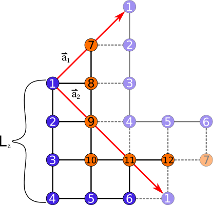
Figure 4: Schematic view of the unit cell for zig-zag length $L_{z}=4$ and labeling of the intra-cell sites. Orange and blue circles indicate the sites with spin up and down, respectively. Solid lines connect sites belonging to one unit cell whereas the dashes line connect sites of neighboring unit cells. The primitive lattice translation vectors $\vec{a}_{1,2}$ are shown explicitly.

The spin orientation of the itinerant electrons is a good quantum number for the problem upon examination. In order to find the time reversal operator, one needs to get a unitary matrix $T$ that satisfies the relation

$${\cal T}^{\dagger}{\cal H}_{\vec{k}}{\cal T}={\cal H}_{-\vec{k}}^{T}.$$ (11)

Note that the transposition on the rhs is equivalent to complex conjugation, so that the whole transformation is antiunitary. Looking at a given block of ${\cal H}_{\vec{k}}$ for $z2$ and $z3$ zig-zag patterns, it is direct to verify that the complex conjugation will only change all the $\vec{k}$ to $-\vec{k}$ and change $\lambda$ to $-\lambda$. If we consider the two orbital flavors as the two independent effective layers of the square lattice then in the absence of the inter-orbital hopping, i.e, when no distortion is present, the change of sign in $\lambda$ can be absorbed by a gauge transformation of the form

$$d_{i,a,\sigma}^{(\dagger)} = -\widetilde{d}_{i,a,\sigma}^{(\dagger)}$$

$$d_{i,b,\sigma}^{(\dagger)} = \tilde{d}_{i,b,\sigma}^{(\dagger)}$$ (12)

where $\tilde{d}^{(\dagger)}$ are the new fermion operators. Since all the hopping processes are orbital-conserving, i.e., there is no effective inter-orbital mixing, the only effect of this gauge transformation is to change the sign of $\lambda$. Thus, the form of the operator ${\cal T}$ is

$${\cal T}=\begin{pmatrix}{\bf 1}_{\downarrow}^{b}&{\bf 0}&{\bf 0}&{\bf 0}\\ {\bf 0}&{\bf 1}_{\uparrow}^{b}&{\bf 0}&{\bf 0}\\ {\bf 0}&{\bf 0}&-{\bf 1}_{\downarrow}^{a}&{\bf 0}\\ {\bf 0}&{\bf 0}&{\bf 0}&-{\bf 1}_{\uparrow}^{a}\end{pmatrix},$$ (13)

where ${\bf 1}$ denotes a unit matrix of the size $N_{\downarrow}$ and the indices are left to indicate spin/orbital sector. Since the matrix is purely real we also observe that $T^{2}=1$.

Another important non-spatial symmetry is that one associated to the sublattice or chiral-like symmetry. Nevertheless, due to the intrinsic antiferromagnetic structure of the zig-zag pattern, one can find a unitary operator ${\cal S}_{k_{1}}$ that anticommutes with Hamiltonian but is explicitly momentum dependent as

$${\cal S}_{k_{1}}^{\dagger}{\cal H}_{\vec{k}}{\cal S}_{k_{1}}=-{\cal H}_{\vec{k}}\,.$$ (14)

In our case such symmetry occurs only at half-filling and arises from the two sublattice structure of the two magnetic domains within a unit cell as marked with different colors in Fig. 4. As one can deduce from the figure, in order to move from one domain to another one, a translation $\vec{a}_{1}$ is needed. For this reason, the operator $S_{k_{1}}$ depends on the quasimomentum $k_{1}$ and has non-zero blocks that connect opposite spin domains within the same orbital sectors, i.e.,

$${\cal S}_{k_{1}}=\begin{pmatrix}{\bf 0}&{\bf S}_{k_{1}}&{\bf 0}&{\bf 0}\\ {\bf S}_{k_{1}}^{\dagger}&{\bf 0}&{\bf 0}&{\bf 0}\\ {\bf 0}&{\bf 0}&{\bf 0}&{\bf S}_{k_{1}}\\ {\bf 0}&{\bf 0}&{\bf S}_{k_{1}}^{\dagger}&{\bf 0}\end{pmatrix},$$ (15)

with

$${\bf S}_{k_{1}}=e^{-i\frac{k_{1}}{2}}\begin{pmatrix}-1&0&0&\cdots&0\\ 0&1&0&\cdots&0\\ 0&0&-1&\cdots&0\\ \vdots&\vdots&\vdots&\ddots&0\\ 0&0&0&0&1\end{pmatrix}.$$ (16)

As we see, apart from the change of the spin-domain there is a phase factor of $e^{-i\frac{k_{1}}{2}}$ appearing with alternating sign $(-1)^{i}$ as we go along the zig-zag segment (from site $i=1$ to $i=8$ in Fig. 4). The alternation is necessary to change the signs of the allowed hoppings that are along the bonds of the square lattice. Here, the chiral symmetry is present only because the zig-zag sublattice structure of the magnetic domains is compatible with the natural two-sublattice structure of the square lattice. Finally, the last non-spatial symmetry is the particle-hole (PHS) of charge conjugation symmetry. As for the chirality, the particle-hole operator is also momentum dependent and satisfies the relation

$${\cal C}_{k_{1}}^{\dagger}{\cal H}_{\vec{k}}{\cal C}_{k_{1}}=-{\cal H}_{-\vec{k}}^{T}.$$ (17)

Such condition implies that if both TRS and sublattice symmetry exist then the charge conjugation is their product, ${\cal C}_{k_{1}}={\cal S}_{k_{1}}\cdot{\cal T}$. It is direct to check that despite the $k$ - dependence in ${\cal S}_{k_{1}}$ we have ${\cal C}^{2}=1$ (in case of the $k$-dependent antiunitary operator this means ${\cal C}_{k_{1}}{\cal C}_{-k_{1}}^{\star}\equiv 1$, where star is complex conjugation).

B.2 Spatial symmetries in a cubic system

The reflection plane for a zig-zag pattern with size $L_{z}=2,3$ is shown in Fig. 1(a)-(b) and can be easily constructed for any $L_{z}$. Its direction is diagonal with respect to the cubic axes so it interchanges the hoppings along the $a$ and $b$ symmetry directions. Such transformation, then, requires an interchange of the orbitals $a$ and $b$ to preserve the connectivity of the system before performing the reflection. Finally, such interchange effectively modifies the sign of $\lambda$ so one can again introduce a gauge transformation as given by Eq. (12). Since the elementary cell of the zig-zag system shown in Fig. 1(a)-(b) is not left invariant by the reflection (one can fix it by an alternative definition of the elementary cell or by taking the square unit cell) the reflection operator depends on quasimomentum $k_{2}$ and has the form

$${\cal R}_{k_{2}}=\begin{pmatrix}{\bf 0}&{\bf 0}&{\bf R}_{k_{2}}&{\bf 0}\\ {\bf 0}&{\bf 0}&{\bf 0}&{\bf{\bf R}}_{k_{2}}\\ -{\bf{\bf R}}_{k_{2}}&{\bf 0}&{\bf 0}&{\bf 0}\\ {\bf 0}&-{\bf{\bf R}}_{k_{2}}&{\bf 0}&{\bf 0}\end{pmatrix},$$ (18)

with $N_{\downarrow}\times N_{\downarrow}$ blocks given by

$${\bf R}_{k_{2}}=\begin{pmatrix}i&0&0&\cdots&0&0\\ 0&0&0&\cdots&0&ie^{ik_{2}}\\ 0&0&0&\cdots&ie^{ik_{2}}&0\\ 0&0&ie^{ik_{2}}&\cdots&0&0\\ 0&ie^{ik_{2}}&0&\cdots&0&0\end{pmatrix}.$$ (19)

This is a unitary matrix satisfying the following relation with the Hamiltonian

$${\cal R}_{k_{2}}^{\dagger}{\cal H}_{k_{1},k_{2}}{\cal R}_{k_{2}}={\cal H}_{k_{1},-k_{2}}.$$ (20)

Despite the dependence on $k_{2}$ the eigenvectors of ${\cal R}_{k_{2}}$ can be found as not depending on $k_{2}$ and its diagonal form is given by the equation,

$${\cal U}^{\dagger}{\cal R}_{k_{2}}{\cal U}=\begin{pmatrix}\mathbf{1}_{2}&{\bf 0}&{\bf 0}&{\bf 0}\\ {\bf 0}&e^{ik_{2}}\mathbf{1}_{2N_{\downarrow}-2}&{\bf 0}&{\bf 0}\\ {\bf 0}&{\bf 0}&-\mathbf{1}_{2}&{\bf 0}\\ {\bf 0}&{\bf 0}&{\bf 0}&-e^{ik_{2}}\mathbf{1}_{2N_{\downarrow}-2}\end{pmatrix},$$ (21)

where ${\cal U}$ is the eigenbasis and the blocks are the unity matrices of size $2$ or $2N_{\downarrow}-2$. We note that for any zig-zag segment length there are two eigenvalues of amplitude $2$, and other two with value $-2$ while the remaining part of the spectrum is given by $\pm e^{ik_{2}}$. The spectrum is chiral in the sense that for any eigenvalue there is a partner with opposite energy. In the reflection planes $k_{2}=0,\pi$ the reflection operator becomes a symmetry for the Hamiltonian, i.e.

$$\left[{\cal H}_{k_{1},0(\pi)},{\cal R}_{0(\pi)}\right]=0$$ (22)

and the $k$-dependence in the spectrum of ${\cal R}_{k_{2}}$ vanishes, being equal to $+1$ at $k_{2}=0$ and $-1$ at $k_{2}=\pi$.

A less straightforward spatial symmetry is that provided by the non-symmorphic glide transformation. It is obtained from the product of a normal reflection with a reflection plane being perpendicular to the one involved in ${\cal R}_{k_{2}}$ and a translation $\vec{t}$ in a direction parallel to the reflection plane. One can easily find that for any zig-zag segment length it is always given by $\vec{t}=\frac{1}{2}\vec{a}_{2}$. The action of the glide operation is shown in Fig.1(a)-(b). We observe that for any zig-zag with even $L_{z}$ both the reflection and translation of the non-primitive lattice vector do not map the original square lattice into itself, only their product does it. Similarly to the regular reflection the glide symmetry is given by a unitary matrix that is mixing the $a$ and $b$ orbitals with a block structure,

$${\cal R}_{k_{1},k_{2}}^{t}=\begin{pmatrix}{\bf 0}&{\bf 0}&-{\bf R}_{k_{1},k_{2}}^{\mathbf{t}}&{\bf 0}\\ {\bf 0}&{\bf 0}&{\bf 0}&-e^{ik}{\bf{\bf R}}_{k_{1},k_{2}}^{\mathbf{t}}\\ {\bf{\bf R}}_{k_{1},k_{2}}^{\mathbf{t}}&{\bf 0}&{\bf 0}&{\bf 0}\\ {\bf 0}&e^{ik}{\bf{\bf R}}_{k_{1},k_{2}}^{\mathbf{t}}&{\bf 0}&{\bf 0}\end{pmatrix},$$ (23)

and the blocks given by the sub-blocks of the size $L_{z}-1\equiv N_{\downarrow}/2$,

$${\bf{\bf R}}_{k_{1},k_{2}}^{\mathbf{t}}=\begin{pmatrix}\mathbf{0}&ie^{-i\frac{k_{2}}{2}}\mathbf{1}_{L_{z}-1}\\ ie^{i\frac{k_{2}}{2}}\mathbf{1}_{L_{z}-1}&\mathbf{0}\end{pmatrix}.$$ (24)

${\cal R}_{k_{1},k_{2}}^{t}$ carries the intrinsic dependence on both quasimomenta that is a direct consequence of the non-symmorphic nature of the glide. One cannot find a unit cell that would map onto itself under such an operation. The relation with the Hamiltonian is the same as for a normal reflection mapping $k_{1}$ into $-k_{1}$, i.e.,

$${\cal R}_{k_{1},k_{2}}^{t\dagger}{\cal H}_{k_{1},k_{2}}{\cal R}_{k_{1},k_{2}}^{t}={\cal H}_{-k_{1},k_{2}}.$$ (25)

The glide operator ${\cal R}_{k_{1},k_{2}}^{t}$ has eigenvectors that depend only on $k_{2}$ and eigenvalues that depend only on $k_{1}$, thus its diagonal form is given by the equation

$${\cal V}_{k_{2}}^{\dagger}{\cal R}_{k_{1},k_{2}}^{t}{\cal V}_{k_{2}}=\begin{pmatrix}{\bf 1}_{N_{\downarrow}}&{\bf 0}&{\bf 0}&{\bf 0}\\ {\bf 0}&e^{ik_{1}}{\bf{\bf 1}}_{N_{\downarrow}}&{\bf 0}&{\bf 0}\\ {\bf 0}&{\bf 0}&-{\bf 1}_{N_{\downarrow}}&{\bf 0}\\ {\bf 0}&{\bf 0}&{\bf 0}&-e^{ik_{1}}{\bf{\bf 1}}_{N_{\downarrow}}\end{pmatrix},$$ (26)

where ${\cal V}_{k_{2}}$ is the eigenbasis and the blocks are the unity matrices of the size $N_{\downarrow}$. In the glide planes $k_{1}=0,\pi$ the glide operator becomes a symmetry of the Hamiltonian, i.e.

$$\left[{\cal H}_{0(\pi),k_{2}},{\cal R}_{0(\pi),k_{2}}^{t}\right]=0,$$ (27)

and the $k$-dependent eigenvalues change the sign when going from one glide plane to the other.

Having two reflection-like operators, as given by Eqs. (20) and Eq. (25), one can immediately construct an inversion operator ${\cal I}_{k_{1},k_{2}}$ satisfying,

$${\cal I}_{k_{1},k_{2}}^{\dagger}{\cal H}_{k_{1},k_{2}}{\cal I}_{k_{1},k_{2}}={\cal H}_{-k_{1},-k_{2}}.$$ (28)

Looking at Eqs. (20) and (25) we argue that the inversion operator has the form

$${\cal I}_{k_{1},k_{2}}\equiv-e^{-i\frac{k_{2}}{2}}{\cal R}_{k_{2}}{\cal R}_{k_{1},-k_{2}}^{t},$$ (29)

where the phase factor is chosen only for convenience. We note that the operators in the product are taken at opposite $k_{2}$ because inserting ${\cal I}_{k_{1},k_{2}}$ into Eq. (28) the first action is on the Hamiltonian with ${\cal R}_{k_{2}}$ which gives us ${\cal H}_{k_{1},-k_{2}}$. Then, if we want to connect with ${\cal H}_{-k_{1},-k_{2}}$ we have to use glide operator at point $(k_{1},-k_{2})$. Unlike the reflection and glide, the inversion does not mix the orbital sectors and its block structure is

$${\cal I}_{k_{1},k_{2}}=\begin{pmatrix}\mathbf{I}_{k_{2}}&{\bf 0}&{\bf 0}&{\bf 0}\\ {\bf 0}&e^{ik}\mathbf{I}_{k_{2}}&{\bf 0}&{\bf 0}\\ {\bf 0}&{\bf 0}&\mathbf{I}_{k_{2}}&{\bf 0}\\ {\bf 0}&{\bf 0}&{\bf 0}&e^{ik}\mathbf{I}_{k_{2}}\end{pmatrix},$$ (30)

with $\mathbf{I}_{k_{2}}$ defined bythe diagonal sub-blocks of the size $L_{z}$ and $L_{z}-2$

$$\mathbf{I}_{k_{2}}=\begin{pmatrix}\mathbf{P}_{L_{z}}&\mathbf{0}\\ \mathbf{0}&e^{ik_{2}}\mathbf{P}_{L_{z}-2}\end{pmatrix}.$$ (31)

These blocks correspond to the vertical and horizontal sections of the spin down/up segment in the unit cell, being the sites $i=1,2,3,4$ and $i=5,6$ for $L_{z}=4$ unit cell as shown in Fig. 4. Finally, ${\bf P}_{n}$ is a simple reflection operator for these straight sections of a zig-zag pattern given by $n\times n$ antidiagonal matrix,

$$\mathbf{P}_{n}=\begin{pmatrix}0&0&\cdots&0&1\\ 0&0&\cdots&1&0\\ 0&1&\cdots&0&0\\ 1&0&\cdots&0&0\end{pmatrix}.$$ (32)

Note that any multiplication of a glide, or a reflection with a translation, with an ordinary reflection, the resulting inversion does not contain a dependence on a translation vector. Indeed, looking at Fig. 1(a)-(b) we can easily find inversion centers for zig-zags with $L_{z}=2$ and $L_{z}=3$. The $k$-dependence in ${\cal I}_{k_{1},k_{2}}$ comes from the fact that the selected unit cell does not map onto itself under the inversion. Hence, one can easily check that it is not possible to find a unit cell which is compatible with inversion for any segment length $L_{z}$. The case of even and odd $L_{z}$ are qualitatively different because for even $L_{z}$ the inversion center does not coincide with any lattice site whereas for odd $L_{z}$ it is a central site in any vertical or horizontal section of a zig-zag. For this reason the spectrum of ${\cal I}_{k_{1},k_{2}}$ for zig-zags with even segment length $L_{z}$ is different than for odd $L_{z}$. For even $L_{z}$ we have a chiral spectrum of the form,

$$\left\{\left\{1\right\}^{L_{z}}\!\!,\left\{-1\right\}^{L_{z}}\!\!,\left\{e^{ik_{1}}\right\}^{L_{z}}\!\!,\left\{-e^{ik_{1}}\right\}^{L_{z}}\!\!,\left\{e^{ik_{2}}\right\}^{L_{z}}\!\!,\right.$$

$$\left.\left\{-e^{ik_{2}}\right\}^{L_{z}}\!\!,\left\{e^{i(k_{1}\!+\!k_{2})}\right\}^{L_{z}\!-\!2}\!\!,\left\{-e^{i(k_{1}\!+\!k_{2})}\right\}^{L_{z}\!-\!2}\right\}\!,\quad$$

where the notation means that, e.g., the eingevalue $1$ is $L_{z}$-fold. For odd $L_{z}$ the spectrum has different number of positive and negative entries, i.e.

$$\left\{\left\{1\right\}^{L_{z}\!+\!1}\!\!,\left\{-1\right\}^{L_{z}\!-\!1}\!\!,\left\{e^{ik_{1}}\right\}^{L_{z}\!+\!1}\!\!,\left\{-e^{ik_{1}}\right\}^{L_{z}\!-\!1}\!\!,\left\{e^{ik_{2}}\right\}^{L_{z}\!-\!1}\!,\right.$$

$$\left.\left\{-e^{ik_{2}}\right\}^{L_{z}\!-\!3}\!\!,\left\{e^{i(k_{1}\!+\!k_{2})}\right\}^{L_{z}\!-\!1}\!\!,\left\{-e^{i(k_{1}\!+\!k_{2})}\right\}^{L_{z}\!-\!3}\right\}\!.\quad\quad$$

For odd $L_{z}$ we can always put electrons in the inversion centers that coincide with physical sites of the system. There are four inversion centers in each unit cell and two orbitals per site so in this way we can obtain eight eigenstates of ${\cal I}_{k_{1},k_{2}}$ with positive eigenvalues, $\left\{1,e^{ik_{1}},e^{ik_{2}},e^{i(k_{1}+k_{2})}\right\}$, all of them being double degenerate. This observation explains why there are more positive eigenvalues then negative for the case of odd $L_{z}$. Note that despite the $k$-dependence in the eigenvalues, the eigenvectors of ${\cal I}_{k_{1},k_{2}}$ are $k$-independent for any $L_{z}$.

B.3 Commutation relations of spacial and non-spatial symmetries

It is not obvious at first glance that the reflection and the glide operators commute. Calculating their commutator one has to always bear in mind that it is the relation to the Hamiltonian that matters, so it is crucial to update the $\vec{k}$ points for which we consider the symmetry operators. For instance, one can show that the operation of reflection and glide does not depend from their order with respect to the Hamiltonian which means that

$${\cal R}_{k_{2}}{\cal R}_{k_{1},-k_{2}}^{t}-{\cal R}_{k_{1},k_{2}}^{t}{\cal R}_{k_{2}}\equiv 0.$$ (33)

Thus, similarly one can demonstrate that the inversion operator commutes with the above operators. Concerning the relation with respect to the time reversal operation one finds that both normal reflection and glide commute with ${\cal T}$, that is

$${\cal R}_{k_{2}}{\cal T}-{\cal T}{\cal R}_{-k_{2}}^{\star}\equiv 0,$$ (34)

and

$${\cal R}_{k_{1},k_{2}}^{t}{\cal T}-{\cal T}{\cal R}_{-k_{1},-k_{2}}^{t\star}\equiv 0,$$ (35)

where the symbol star indicate complex conjugation. Thus, we conclude that the same property holds for the inversion. Finally, concerning the chirality (sublattice) symmetry we find that the reflection commutes with ${\cal S}_{k_{1}}$,

$${\cal R}_{k_{2}}{\cal S}_{k_{1}}-{\cal S}_{k_{1}}{\cal R}_{k_{2}}\equiv 0,$$ (36)

and the glide anticommutes or commutes with ${\cal S}_{k_{1}}$ for even or odd $L_{z}$ respectively, i.e.

$${\cal R}_{k_{1},k_{2}}^{t}{\cal S}_{k_{1}}+(-1)^{L_{z}}{\cal S}_{k_{1}}{\cal R}_{k_{1},k_{2}}^{t}\equiv 0.$$ (37)

Intuitively one can argue that the chirality symmetry is related to the two-sublattice structure of the problem. Since under reflection a site belonging to one sublattice transforms to another site from the same sublattice we get the vanishing commutator in (36). On the other hand, looking at Fig. 4, we notice that for $L_{z}=2$ the glide does mix the sites from different sublattices hence one gets a vanishing anticommutator. It is easy to check that this happens for any even $L_{z}$ whereas for the odd ones we always get a vanishing commutation relation. Finally, we note that since all spacial symmetries commute with time reversal, their commutation relation with particle-hole symmetry is the same as that one with the chirality.

B.4 Combined symmetries

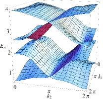
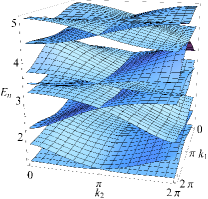
Figure 5: Positive-energy bands of the undistorted (cubic) zig-zag $L_{z}=2$ (left) and $L_{z}=3$ (right) systems. The negative-energy bands can be recovered by reflection with respect to zero energy due to the chirality ${\cal S}_{k_{1}}$. We note that the bands appear in $(2L_{z}-2)$ pairs and every pair has a 1D crossing line at $k_{2}=\pi$ due to effective Kramers degeneracy occurring at any cut along $k_{2}$ direction. These pairs are Kramers doublets at $k_{2}=\pi$. The spectrum for $L_{z}=2$ has two Dirac points in the glide plane $k_{1}=\pi$.

Having both spatial and non-spatial symmetries we can construct various combined symmetries by taking their products. Here, we will focus only on antiunitary symmetries constructed by combining time reversal operator with reflection, glide and inversion. We start with the reflection, defining ${\cal T}_{k_{2}}^{(1)}$ as

$${\cal T}_{k_{2}}^{(1)}\equiv{\cal R}_{k_{2}}{\cal T},$$ (38)

we obtain a time reversal operator acting in the 1D cuts of BZ parallel to the $k_{1}$ ($k_{1}$-cuts) axis,

$${\cal T}_{k_{2}}^{(1)\dagger}{\cal H}_{k_{1},k_{2}}{\cal T}_{k_{2}}^{(1)}={\cal H}_{-k_{1},k_{2}}^{T}.$$ (39)

In the same way using glide operator we can define ${\cal T}_{k_{1},k_{2}}^{(2)}$ as,

$${\cal T}_{k_{1},k_{2}}^{(2)}\equiv{\cal R}_{k_{1},k_{2}}^{t}{\cal T},$$ (40)

which is a time reversal operator acting in the cuts parallel to the $k_{2}$ axis ($k_{2}$-cuts),

$${\cal T}_{k_{1},k_{2}}^{(2)\dagger}{\cal H}_{k_{1},k_{2}}{\cal T}_{k_{1},k_{2}}^{(2)}={\cal H}_{k_{1},-k_{2}}^{T}.$$ (41)

Similarly, we can combine time reversal with the inversion operator by introducing the operator ${\cal K}_{k_{1},k_{2}}$ as given by

$${\cal K}_{k_{1},k_{2}}\equiv{\cal I}_{k_{1},k_{2}}{\cal T},$$ (42)

whose action on the Hamiltonian yields its transpose or complex conjugate

$${\cal K}_{k_{1},k_{2}}^{\dagger}{\cal H}_{k_{1},k_{2}}{\cal K}_{k_{1},k_{2}}={\cal H}_{k_{1},k_{2}}^{T}.$$ (43)

Thus, we can denote ${\cal K}_{k_{1},k_{2}}$ as a pure conjugation operator. A close inspection at the powers of these three anti-unitary symmetries, for $k_{1}$-cuts in the Brillouin zone, and for the pure conjugation, we find that these square to give the unity

$${\cal T}_{k_{2}}^{(1)}{\cal T}_{k_{2}}^{(1)\star}\equiv 1,\quad{\cal K}_{k_{1},k_{2}}{\cal K}_{k_{1},k_{2}}^{\star}\equiv 1,$$ (44)

on the other hand, for $k_{2}$-cuts we obtain a $k$-dependent result,

$${\cal T}_{k_{1},k_{2}}^{(2)}{\cal T}_{k_{1},-k_{2}}^{(2)\star}\equiv e^{-ik_{2}}.$$ (45)

This means that in two time-reversal points of a given $k_{2}$-cut, namely $k_{2}=0$ and $k_{2}=\pi$ we have $({\cal T}^{(2)})^{2}=1$ and $({\cal T}^{(2)})^{2}=-1$. Thus, one can conclude that for every $k_{2}$-cut the point $k_{2}=\pi$ is a Kramers degenerate point. Note that this is a surprising result as the problem with which we deal is spinless and also because the other time-reversal point in the Brillouin zone is not Kramers degenerate. The result on the bands of any $L_{z}$ zig-zag system is interesting as at $k_{2}=\pi$ and any $k_{1}$ every band is twice degenerate. To explicitly demonstrate this property, we present the 1D bands crossings for $L_{z}=2$ and $L_{z}=3$ in Fig. 5.

B.5 Gauging away $k$-dependecies in all symmetries operators

As we noticed in the previous Sections, due to the structure of the unit cell and the presence of the non-symmorphic glide symmetry, most of the spatial and non-spatial symmetries are $k$-dependent. It is worth and interesting to underline that these $k$-dependences can be simultaneously gauged away for any zig-zag segment length $L_{z}$ by a transformation of the form

$${\cal G}_{\vec{k}}=\begin{pmatrix}{\bf G}_{\downarrow}&{\bf 0}&{\bf 0}&{\bf 0}\\ {\bf 0}&{\bf G}_{\uparrow}&{\bf 0}&{\bf 0}\\ {\bf 0}&{\bf 0}&{\bf G}_{\downarrow}&{\bf 0}\\ {\bf 0}&{\bf 0}&{\bf 0}&{\bf G}_{\uparrow}\end{pmatrix},$$ (46)

with diagonal blocks ${\bf G}_{\downarrow}$and ${\bf G}_{\uparrow}$ of the size $N_{\downarrow}=N_{\uparrow}=2L_{z}-2$,

$${\bf G}_{\downarrow}=e^{-ik_{1}}\begin{pmatrix}1&0&0&\cdots&0\\ 0&e^{i\frac{1}{N_{\downarrow}}k_{2}}&0&\cdots&0\\ 0&0&e^{i\frac{2}{N_{\downarrow}}k_{2}}&\cdots&0\\ \vdots&\vdots&\vdots&\ddots&0\\ 0&0&0&0&e^{i\frac{N_{\downarrow}-1}{N_{\downarrow}}k_{2}}\end{pmatrix},$$ (47)

and

$${\bf G}_{\uparrow}=e^{i\frac{k_{1}}{2}}{\bf G}_{\downarrow},$$ (48)

corresponding to the domains of spin up/down in the unit call. Note that these matrices are the same for the orbital $a$ and orbital $b$ sector. The Hamiltonian transforms as a linear operator under the basis rotation, i.e.

$${\cal\tilde{H}}_{\vec{k}}\equiv{\cal G}_{\vec{k}}^{\dagger}{\cal H}_{\vec{k}}{\cal G}_{\vec{k}},$$ (49)

where tilde indicates the operator in the gauge transformed basis. Now, if we require that the reflection operator in the gauge transformed basis, i.e., ${\cal\tilde{R}}$ acts as a reflection operator with respect to ${\cal\tilde{H}}_{\vec{k}}$, i.e.,

$$\tilde{{\cal R}}{}^{\dagger}\tilde{{\cal H}}_{k_{1},k_{2}}\tilde{{\cal R}}=\tilde{{\cal H}}_{k_{1},-k_{2}},$$ (50)

we easily find that ${\cal\tilde{R}}$ should have the following form

$${\cal\tilde{R}}\propto{\cal G}_{k_{1},k_{2}}^{\dagger}{\cal R}_{k_{2}}{\cal G}_{k_{1},-k_{2}},$$ (51)

where the complex prefactor can be chosen in such a way to completely remove any $k$-dependence in ${\cal\tilde{R}}$. Similarly, we can proceed for the glide,

$${\cal\tilde{R}}^{t}\propto{\cal G}_{k_{1},k_{2}}^{\dagger}{\cal R}_{k_{1},k_{2}}^{t}{\cal G}_{-k_{1},k_{2}},$$ (52)

and for the other non-spatial symmetries. For instance time reversal operator,

$${\cal\tilde{T}}\propto{\cal G}_{k_{1},k_{2}}^{\dagger}{\cal T}{\cal G}_{-k_{1},-k_{2}}^{\star},$$ (53)

where the gauge matrix on the right is taken with complex conjugate. While for the chirality we have that

$${\cal\tilde{S}}\propto{\cal G}_{k_{1},k_{2}}^{\dagger}{\cal S}_{k_{2}}{\cal G}_{k_{1},k_{2}},$$ (54)

and transforms through a simple basis rotation. The rest of the symmetries can be constructed by taking the product of the above operators, i.e.,

$$\tilde{{\cal I}}={\cal\tilde{R}}{\cal\tilde{R}}^{t}={\cal\tilde{R}}^{t}{\cal\tilde{R}},$$ (55)

to get the inversion and

$$\tilde{{\cal C}}={\cal\tilde{T}}{\cal\tilde{S}}^{\star}={\cal\tilde{S}}{\cal\tilde{T}},$$ (56)

to get charge conjugation. Note that the spatial symmetries and the time reversal do not transform as linear operators under basis rotation. For this reason their spectra are different in the gauge transformed basis with respect to the initial one and their commutation relations could be different as well. Accidentally, we find that the commutation relations remain the same as shown in previous Section.

Finally, we stress that the consequence of the removal of the $k$-dependencies from the symmetries operators is to alter the periodicity of the Hamiltonian in the momentum space. One find that for a given $L_{z}$ the period in $k_{1}$ is always doubled, i.e., $\tilde{{\cal H}}_{k_{1}+4\pi,k_{2}}=\tilde{{\cal H}}_{k_{1},k_{2}}$ whereas that one in $k_{2}$ is increased $N_{\downarrow}$ - times. This effect can be captured by what we call the shift operator. We find that however the period is elongated the old period of $2\pi$ survives up to a basis rotation described by a unitary shift operator $\chi$. For $k_{1}$ we find that,

$$\tilde{{\cal H}}_{k_{1}+2\pi,k_{2}}=\chi_{1}^{\dagger}\tilde{{\cal H}}_{k_{1},k_{2}}\chi_{1},$$ (57)

where $\chi_{1}$ can be found as a ’$2\pi$-basis mismatch’ of the gauge matrix, i.e.,

$$\chi_{1}\propto{\cal G}_{k_{1},k_{2}}^{\dagger}{\cal G}_{k_{1}+2\pi,k_{2}}.$$ (58)

One finds that

$$\left(\chi_{1}\right)^{2}=1,$$ (59)

meaning that after two $2\pi$-shifts in $k_{1}$ we recover the same Hamiltonian $\tilde{{\cal H}}_{k_{1},k_{2}}$. Similarly for $k_{2}$ we observe,

$$\tilde{{\cal H}}_{k_{1},k_{2}+2\pi}=\chi_{2}^{\dagger}\tilde{{\cal H}}_{k_{1},k_{2}}\chi_{2},$$ (60)

with $\chi_{2}$ unitary shift operator having the form of

$$\chi_{2}\propto{\cal G}_{k_{1},k_{2}}^{\dagger}{\cal G}_{k_{1},k_{2}+2\pi},$$ (61)

and becoming unity after $N_{\downarrow}$ applications

$$\left(\chi_{2}\right)^{N_{\downarrow}}=1.$$ (62)

B.6 Gauging away $k$-dependence of the reflection operator

The gauge transformation described in Sec. B.5 makes all the symmetry opearators $k$-independent but concomitantly one has to increase the effective Brillouin zone of the Hamiltonian. This is caused by the fact that the unit cell is not left invariant by any of the symmetries of the whole system. In the case of glide, inversion and chirality symmetries it is in indeed impossible to define a unit cell that would map onto itself under their action. However, in the case of reflection this transformation is possible. Another operating scheme would be to choose a square unit cell, as shown in Fig. 1(a)-(b), but in this way we increase the dimensionality of the operators and create artificial symmetries coming from the multiple copies of the elementary cell. The other solution, which is much more convenient, is to slightly modify the elementary unit cell shown in Fig. 4. One has to remind that every physical site in the lattice has two orbital flavors so the resulting system can be also mapped into an effective bilayer. The reflection can be seen as a $\pi$-rotation of the bilayer with axis along the $\vec{a}_{1}$ direction. Thus a reflection-invariant unit cell can be constructed by taking the original cell for orbital $b$ and for orbital $a$ one has to move the first two sites ($i=1,7$ in Fig. 4) of the vertical segments after the last two sites ($i=6,12$ in Fig. 4) of the horizontal segments. This can be realized by a gauge transformation of the type

$${\cal G}_{k_{2}}^{{\cal R}}=\begin{pmatrix}{\bf 1}_{\downarrow}^{b}&{\bf 0}&{\bf 0}&{\bf 0}\\ {\bf 0}&{\bf 1}_{\uparrow}^{b}&{\bf 0}&{\bf 0}\\ {\bf 0}&{\bf 0}&{\bf G}_{\downarrow}^{R}&{\bf 0}\\ {\bf 0}&{\bf 0}&{\bf 0}&{\bf G}_{\uparrow}^{R}\end{pmatrix},$$ (63)

with two identical sub-blocks for orbital $a$ segment,

$${\bf G}_{\downarrow,\uparrow}^{R}=\begin{pmatrix}e^{-ik_{2}}&0&0&\cdots&0\\ 0&1&0&\cdots&0\\ 0&0&1&\cdots&0\\ \vdots&\vdots&\vdots&\ddots&0\\ 0&0&0&0&1\end{pmatrix},$$ (64)

carrying the gauge for the first sites of the vertical segment. After the covariant transformation of the reflection operator, i.e., ${\cal R}_{k_{2}}\to{\cal G}_{k_{2}}^{{\cal R}\dagger}{\cal R}_{k_{2}}{\cal G}_{-k_{2}}^{{\cal R}}$ and extracting global phase factor we find it completely $k$-independent.

B.7 Gauging away $k_{1}$-dependence of the glide symmetry operator

Another gauge transformation can be found to demonstrate that the glide operator ${\cal R}_{\vec{k}}^{t}$ is dependent only on $k_{2}$ without affecting the periodicity of the Hamiltonian. Again, this solution is equivalent to a modification of the elementary unit cell shown in Fig. 4. Treating the $a$ and $b$ orbital degrees of freedom as two layers one can treat the glide as a $\pi$-rotation of the bilayer with axis along the $\vec{a}_{2}$ direction followed by a shift of $\vec{a}_{2}/2$ . Thus, a way to construct a unit cell which is mostly compatible with a glide is to take the original cell for the orbital $a$ and for the orbital $b$, and then shift the spin down domain by $\vec{a}_{1}$ (see Fig. 4). In this way we obtain a gauge transformation of the form

$${\cal G}_{k_{1}}^{{\cal R}^{t}}=\begin{pmatrix}{\bf G}_{\downarrow}^{R^{t}}&{\bf 0}&{\bf 0}&{\bf 0}\\ {\bf 0}&{\bf 1}_{\uparrow}^{b}&{\bf 0}&{\bf 0}\\ {\bf 0}&{\bf 0}&{\bf 1}_{\downarrow}^{a}&{\bf 0}\\ {\bf 0}&{\bf 0}&{\bf 0}&{\bf 1}_{\uparrow}^{a}\end{pmatrix},$$ (65)

with one non-trivial subblock,

$${\bf G}_{\downarrow}^{R^{t}}=\begin{pmatrix}e^{-ik_{1}}&0&0&\cdots&0\\ 0&1&0&\cdots&0\\ 0&0&1&\cdots&0\\ \vdots&\vdots&\vdots&\ddots&0\\ 0&0&0&0&1\end{pmatrix},$$ (66)

carrying the gauge for the spin down domain of orbitals $b$. After the covariant transformation of the glide operator, i.e., ${\cal R}_{\vec{k}}^{t}\to{\cal G}_{k_{1}}^{{\cal R}^{t}\dagger}{\cal R}_{\vec{k}}^{t}{\cal G}_{-k_{1}}^{{\cal R}^{t}}$ and extracting global phase factor we find it dependent only on $k_{2}/2$ (due to the $\vec{a}_{2}/2$ shift) in such a way that it eigenvalues are $k$-independent taking values $g_{\pm}=\pm 1$. The dependence on $k_{2}$ of the eigenbasis is such that the eigenvectors with $g_{+}$ eigenvalues at fixed $k_{2}$ become the $g_{-}$ eigenvectors at $k_{2}+2\pi$.

B.8 Hamiltonians and k-independent symmetries for $L_{z}=2,3$

We will focus on undistorted zig-zag systems where the only non-zero hopping amplitudes are $t_{\hat{a},i}^{bb}=t_{\hat{b},i}^{aa}=-t$ and where we set $t=1$ as the energy unit. For zig-zag segment lengths $L_{z}=2$ and $L_{z}=3$ the Hamiltonians are $8\times 8$ and $16\times 16$ hermitian matrices, respectively. Thus, it is convenient to use the product basis of $3$ and $4$ Pauli matrices to show the exact form of the Hamiltonians and their symmetries in these two cases. For $L_{z}=2$ we will decompose the operators in basis of $64$ hermitian matrices whose building blocks are pseudospins $S=1/2$ defined on three artificial sites, i.e.

$$\sigma_{1}^{\alpha}=\sigma^{\alpha}\otimes 1_{2}\otimes 1_{2},\quad\sigma_{2}^{\alpha}=1_{2}\otimes\sigma^{\alpha}\otimes 1_{2},\quad\sigma_{3}^{\alpha}=1_{2}\otimes 1_{2}\otimes\sigma^{\alpha},$$ (67)

with $\alpha=x,y,z$ and $\sigma^{\alpha}$ being a Pauli matrix. Hence, the Hamiltonian in the gauge transformed basis and for the shortest possible zig-zag with $L_{z}=2$ can be represented as

$$\tilde{{\cal H}}_{\vec{k}} = \sin\frac{k_{2}}{2}\left(\sin\frac{k_{1}}{2}\sigma_{3}^{x}+\cos\frac{k_{1}}{2}\sigma_{3}^{y}\right)\sigma_{1}^{z}\sigma_{2}^{x}$$ (68)

$$+ \cos\frac{k_{2}}{2}\left(\sin\frac{k_{1}}{2}\sigma_{3}^{x}-\cos\frac{k_{1}}{2}\sigma_{3}^{x}\right)\sigma_{2}^{x}$$

$$- \cos\frac{k_{2}}{2}\sigma_{3}^{x}-\sin\frac{k_{2}}{2}\sigma_{1}^{z}\sigma_{3}^{y}$$

$$+ J_{H}\sigma_{2}^{z}-\lambda\sigma_{1}^{y}\sigma_{2}^{z}.$$

The spatial symmetries take the form

$${\cal\tilde{R}} = \sigma_{1}^{y},$$

$${\cal\tilde{R}}^{t} = \sigma_{1}^{y}\sigma_{3}^{x},$$

$$\tilde{{\cal I}} = \sigma_{3}^{x},$$ (69)

and the non-spatial symmetries are

$${\cal\tilde{T}} = \sigma_{1}^{z},$$

$${\cal\tilde{S}} = \sigma_{2}^{x}\sigma_{3}^{z},$$

$$\tilde{C} = \sigma_{1}^{z}\sigma_{2}^{x}\sigma_{3}^{z}.$$ (70)

The algebra is completed by the shift operators defined in the previous subsection as

$$\chi_{1} = \sigma_{2}^{z},$$

$$\chi_{2} = \sigma_{3}^{z}.$$ (71)

It is instructive to check that all these operators really satisfy the relevant relations with respect to the Hamiltonian.

Analogically, for $L_{z}=3$ we span a basis of $256$ hermitian matrices whose building blocks are pseudospins $S=1/2$ acting on four artificial sites, i.e.

$$\sigma_{1}^{\alpha}\!=\!\sigma^{\alpha}\!\otimes 1_{2}\otimes 1_{2}\otimes 1_{2}, \sigma_{2}^{\alpha}\!=\!1_{2}\otimes\sigma^{\alpha}\!\otimes 1_{2}\otimes 1_{2},$$

$$\sigma_{3}^{\alpha}\!=\!1_{2}\otimes 1_{2}\otimes\sigma^{\alpha}\!\otimes 1_{2}, \sigma_{4}^{\alpha}\!=\!1_{2}\otimes 1_{2}\otimes 1_{2}\otimes\sigma^{\alpha}\!.$$ (72)

The Hamiltonian in the gauge transformed basis for the zig-zag with $L_{z}=3$ can be represented as

$$\tilde{{\cal H}}_{\vec{k}} \!=\! \frac{1}{2}\sin\frac{k_{2}}{4}\left(\sigma_{4}^{y}\!-\!\sigma_{3}^{x}\sigma_{4}^{y}\!-\!\sigma_{1}^{z}\sigma_{3}^{y}\sigma_{4}^{x}\!-\!\sigma_{1}^{z}\sigma_{3}^{z}\sigma_{4}^{y}\right)$$ (73)

$$\!+\! \frac{1}{2}\cos\frac{k_{2}}{4}\left(-\!\sigma_{4}^{x}\!-\!\sigma_{3}^{x}\sigma_{4}^{x}\!+\!\sigma_{1}^{z}\sigma_{3}^{y}\sigma_{4}^{y}\!+\!\sigma_{1}^{z}\sigma_{3}^{z}\sigma_{4}^{x}\right)$$

$$\!+\! \frac{1}{2}\sin\frac{k_{2}}{4}\sin\frac{k_{1}}{2}\sigma_{2}^{x}\left(\sigma_{3}^{y}\sigma_{4}^{y}\!+\!\sigma_{3}^{z}\sigma_{4}^{x}\!+\!\sigma_{1}^{z}\sigma_{4}^{x}\!+\!\sigma_{1}^{z}\sigma_{3}^{x}\sigma_{4}^{x}\right)$$

$$\!+\! \frac{1}{2}\cos\frac{k_{2}}{4}\sin\frac{k_{1}}{2}\sigma_{2}^{x}\left(\sigma_{3}^{y}\sigma_{4}^{x}\!+\!\sigma_{3}^{z}\sigma_{4}^{y}\!+\!\sigma_{1}^{z}\sigma_{4}^{y}\!-\!\sigma_{1}^{z}\sigma_{3}^{x}\sigma_{4}^{y}\right)$$

$$\!+\! \frac{1}{2}\sin\frac{k_{2}}{4}\cos\frac{k_{1}}{2}\sigma_{1}^{z}\sigma_{2}^{x}\left(\sigma_{3}^{y}\sigma_{4}^{x}\!+\!\sigma_{3}^{z}\sigma_{4}^{y}\!+\!\sigma_{1}^{z}\sigma_{4}^{y}\!-\!\sigma_{1}^{z}\sigma_{3}^{x}\sigma_{4}^{y}\right)$$

$$\!-\! \frac{1}{2}\cos\frac{k_{2}}{4}\cos\frac{k_{1}}{2}\sigma_{1}^{z}\sigma_{2}^{x}\left(\sigma_{3}^{y}\sigma_{4}^{y}\!+\!\sigma_{3}^{z}\sigma_{4}^{x}\!+\!\sigma_{1}^{z}\sigma_{4}^{x}\!+\!\sigma_{1}^{z}\sigma_{3}^{x}\sigma_{4}^{x}\right)$$

$$\!+\! J_{H}\sigma_{2}^{z}-\lambda\sigma_{1}^{y}\sigma_{2}^{z}.$$

The spatial symmetries take the form,

$${\cal\tilde{R}} = \frac{1}{2}\sigma_{1}^{y}\left(\left(1-\sigma_{3}^{x}\right)\left(1-\sigma_{4}^{z}\right)-2\right),$$

$${\cal\tilde{R}}^{t} = \sigma_{1}^{y}\sigma_{3}^{x},$$

$$\tilde{{\cal I}} = \frac{1}{2}\left(\left(1-\sigma_{3}^{x}\right)\left(1+\sigma_{4}^{z}\right)-2\right),$$ (74)

and the non-spatial symmetries are

$${\cal\tilde{T}} = \sigma_{1}^{z},$$

$${\cal\tilde{S}} = \sigma_{2}^{x}\sigma_{4}^{z},$$

$$\tilde{C} = \sigma_{1}^{z}\sigma_{2}^{x}\sigma_{4}^{z},$$ (75)

while the shift operators can be expressed as

$$\chi_{1} = \sigma_{2}^{z},$$

$$\chi_{2} = \frac{1}{\sqrt{2}}\sigma_{3}^{z}\left(i+\sigma_{4}^{z}\right).$$ (76)

Note that, as expected for $L_{z}=3$, $(\chi_{2})^{4}=1$ whereas the lower powers are non-trivial, e.g., $(\chi_{2})^{2}=\sigma_{4}^{z}$. Finally the second and third neighbor hopping $\delta$ is this basis has a form,

$$\tilde{h}(\delta)=\delta\sigma_{2}^{z}\sigma_{3}^{x}\cos\frac{k_{2}}{2}.$$ (77)

One can easily check that it preserves all the symmetries.

B.9 Symmetry in the parameters space

For any zig-zag segment length $L_{z}$ it is possible to find additional symmetries that can be associated to two reflections operators $\tilde{{\cal X}}$ and $\tilde{{\cal Y}}$ and an inversion $\tilde{{\cal Z}}=\tilde{{\cal X}}\tilde{{\cal Y}}$ that act uniquely in the parameters space $(J_{H},\lambda)$. The reflections are active only in the glide plane $k_{1}=0$ and satisfy the relations,

$$\tilde{{\cal X}}{}^{\dagger}\tilde{{\cal H}}_{0,k_{2}}\left(J_{H},\lambda\right)\tilde{{\cal X}} = \tilde{{\cal H}}_{0,k_{2}}\left(\lambda,J_{H}\right),$$

$$\tilde{{\cal Y}}{}^{\dagger}\tilde{{\cal H}}_{0,k_{2}}\left(J_{H},\lambda\right)\tilde{{\cal Y}} = \tilde{{\cal H}}_{0,k_{2}}\left(-\lambda,-J_{H}\right).$$ (78)

Thus we see that the reflection planes in the parameters plane $(J_{H},\lambda)$ are in the direction $J_{H}=\lambda$ and $J_{H}=-\lambda$. The action of the inversion $\tilde{{\cal Z}}$ on the Hamiltonian is obviously,

$$\tilde{{\cal Z}}{}^{\dagger}\tilde{{\cal H}}_{0,k_{2}}\left(J_{H},\lambda\right)\tilde{{\cal Z}}=\tilde{{\cal H}}_{0,k_{2}}\left(-J_{H},-\lambda\right).$$ (79)

The general matrix form of the two reflections in the gauged basis is,

$$\tilde{{\cal X}}=\frac{1}{2}\begin{pmatrix}{\bf 1}_{N_{\downarrow}}&-{\bf 1}_{N_{\downarrow}}&i{\bf 1}_{N_{\downarrow}}&i{\bf 1}_{N_{\downarrow}}\\ -{\bf 1}_{N_{\downarrow}}&{\bf{\bf 1}}_{N_{\downarrow}}&i{\bf 1}_{N_{\downarrow}}&i{\bf{\bf 1}}_{N_{\downarrow}}\\ -i{\bf 1}_{N_{\downarrow}}&-i{\bf 1}_{N_{\downarrow}}&{\bf 1}_{N_{\downarrow}}&-{\bf 1}_{N_{\downarrow}}\\ -i{\bf 1}_{N_{\downarrow}}&-i{\bf{\bf 1}}_{N_{\downarrow}}&-{\bf 1}_{N_{\downarrow}}&{\bf{\bf 1}}_{N_{\downarrow}}\end{pmatrix},$$ (80)

and

$$\tilde{{\cal Y}}=-\frac{1}{2}\begin{pmatrix}-{\bf 1}_{N_{\downarrow}}&{\bf 1}_{N_{\downarrow}}&i{\bf 1}_{N_{\downarrow}}&i{\bf 1}_{N_{\downarrow}}\\ {\bf 1}_{N_{\downarrow}}&-{\bf{\bf 1}}_{N_{\downarrow}}&i{\bf 1}_{N_{\downarrow}}&i{\bf{\bf 1}}_{N_{\downarrow}}\\ -i{\bf 1}_{N_{\downarrow}}&-i{\bf 1}_{N_{\downarrow}}&-{\bf 1}_{N_{\downarrow}}&{\bf 1}_{N_{\downarrow}}\\ -i{\bf 1}_{N_{\downarrow}}&-i{\bf{\bf 1}}_{N_{\downarrow}}&{\bf 1}_{N_{\downarrow}}&-{\bf{\bf 1}}_{N_{\downarrow}}\end{pmatrix}.$$ (81)

Note that the spectra of $\tilde{{\cal X}}$ and $\tilde{{\cal Y}}$ are the same and consist of $N_{\downarrow}$ eigenvalues $-1$ and $3N_{\downarrow}$eigenvalues $1$ which concides with the spectrum of the SU$(2)$ spin interchange operator $X_{12}=\frac{1}{2}(1+\vec{\sigma}_{1}\vec{\sigma}_{2})$ taken $N_{\downarrow}$ times. The spectrum of $\tilde{{\cal Z}}$ consist of eqaul number of $+1$ and $-1$ eigenvalues.

For $L_{z}=2$ and $L_{z}=3$ operators $\tilde{{\cal X}}$, $\tilde{{\cal Y}}$ and ${\cal\tilde{Z}}$ can be written in terms Pauli matrices (67) or (72) as,

$$\tilde{{\cal X}} = \frac{1}{2}\left(1-\sigma_{1}^{y}-\sigma_{1}^{y}\sigma_{2}^{x}-\sigma_{2}^{x}\right),$$

$$\tilde{{\cal{\cal Y}}} = -\sigma_{2}^{x}\tilde{{\cal X}},$$

$$\tilde{{\cal Z}} = -\sigma_{2}^{x}.$$ (82)

For these two shortest zig-zags with $L_{z}=2,3$ we find that the inversion operator $\tilde{{\cal Z}}$ satisfies,

$$\tilde{{\cal Z}}{}^{\dagger}\tilde{{\cal H}}_{k_{1},k_{2}}\left(J_{H},\lambda\right)\tilde{{\cal Z}}=\tilde{{\cal H}}_{k_{1},k_{2}}\left(-J_{H},-\lambda\right),$$ (83)

for any $k$-point whereas only for $L_{z}=2$ we get extra relations for the $\tilde{{\cal X}}$ and $\tilde{{\cal Y}}$ operators in the plane $k_{2}=0$,

$$\tilde{{\cal X}}{}^{\dagger}\tilde{{\cal H}}_{k_{1},0}\left(J_{H},\lambda\right)\tilde{{\cal X}} = \tilde{{\cal H}}_{k_{1},0}\left(\lambda,J_{H}\right),$$

$$\tilde{{\cal Y}}{}^{\dagger}\tilde{{\cal H}}_{k_{1},0}\left(J_{H},\lambda\right)\tilde{{\cal Y}} = \tilde{{\cal H}}_{k_{1},0}\left(-\lambda,-J_{H}\right).$$ (84)

B.10 Multiple glide and reflection operators

An interesting consequence of gauge transformation described in Sec. B.8, related with elongation of Hamiltonian’s period, is multiplication of reflection and glide operators. Have a look at the reflection planes, we easily find that for any $L_{z}$,

$$\left[\tilde{{\cal H}}_{k_{1},0},\tilde{{\cal R}}\right]=0,$$ (85)

but due to the period elongation in $\tilde{{\cal H}}_{k_{1},k_{2}}$ we also find that

$$\left[\tilde{{\cal H}}_{k_{1},\pi},\tilde{{\cal R}}\right]\not=0.$$ (86)

This means that $k_{2}=0$ is the reflection plane for $\tilde{{\cal R}}$ but $k_{2}=\pi$ is not. It is not difficult to guess that the sceond reflection plane should be placed at $k_{2}$ equal to half-period of the new BZ, namely at $k_{2}=N_{\downarrow}\pi$. Indee we find

$$\left[\tilde{{\cal H}}_{k_{1},N_{\downarrow}\pi},\tilde{{\cal R}}\right]=0,$$ (87)

but one may ask what about $k_{2}=\pi,2\pi,\dots(N_{\downarrow}-1)\pi$ , is there any reflection operator for whom these are the reflection planes? The answer is yes, we can define shifted reflection operators ${\cal\tilde{R}}_{\chi}^{(n)}$ in the following way,

$${\cal\tilde{R}}_{\chi}^{(n)}\equiv{\cal\tilde{R}}\left(\chi_{2}\right)^{n},$$ (88)

where $n=1,2,\dots,(N_{\downarrow}-1)$. Their action on Hamiltonian is the following,

$${\cal\tilde{R}}_{\chi}^{(n)\dagger}\tilde{{\cal H}}_{k_{1},k_{2}}{\cal\tilde{R}}_{\chi}^{(n)}=\tilde{{\cal H}}_{k_{1},-k_{2}+2\pi n}.$$ (89)

Now it’s easy to notice that,

$$\left[\tilde{{\cal H}}_{k_{1},n\pi},{\cal\tilde{R}}_{\chi}^{(n)}\right]=\left[\tilde{{\cal H}}_{k_{1},n\pi+N_{\downarrow}\pi},{\cal\tilde{R}}_{\chi}^{(n)}\right]=0,$$ (90)

meaning that planes $k_{2}=n\pi$ and $k_{2}=n\pi+N_{\downarrow}\pi$ are the reflection planes for the shifted reflection operator ${\cal\tilde{R}}_{\chi}^{(n)}$. Note that unlike initial reflection $\tilde{{\cal R}}$ the shifted reflection operators are not hermitian and unitary, they are only unitary. Similarly we can define a shifted glide oprator ${\cal\tilde{R}}_{\chi}^{t}$,

$${\cal\tilde{R}}_{\chi}^{t}\equiv{\cal\tilde{R}}^{t}\chi_{1}.$$ (91)

Here we have only one shifted operator because for any zig-zag $(\chi_{1})^{2}=1$. For this operator the reflection planes are $k_{1}=\pi$ and $k_{1}=3\pi$ whereas for non-shifted ${\cal\tilde{R}}^{t}$ these are $k_{1}=0$ and $k_{1}=2\pi$. Note that the period of gauged Hamiltonian $\tilde{{\cal H}}_{k_{1},k_{2}}$ in $k_{1}$ is $4\pi$ for any $L_{z}$. By taking products of shifted reflection and glide operators we can construct different shifted inversion operators for different inversion points in the enlarged BZ of $\tilde{{\cal H}}_{k_{1},k_{2}}$.

The final conclusion for this Section is that however the $k$-dependence in spatial symmetry operators can be removed by a proper gauge transformation, this dependence reappears in the gauged basis as a multiple definition of these operators for different symmetry-invariant $k$-points.

Appendix C Reducing the Hamiltonian into a purely real matrix form

The combination of the time reversal and inversion transformation leads to the operator ${\cal K}_{\vec{k}}$ defined as,

$${\cal K}_{\vec{k}}\equiv{\cal I}_{\vec{k}}{\cal T},$$ (92)

whose action on the Hamiltonian is to make it transposed or complex conjugated,

$${\cal K}_{\vec{k}}^{\dagger}{\cal H}_{\vec{k}}{\cal K}_{\vec{k}}={\cal H}_{\vec{k}}^{T}.$$ (93)

Thus, we can generally indicate ${\cal K}_{\vec{k}}$ as a conjugation operator. Due to its structure and on the property of $\cal I$ and $\cal T$, we find that the square of ${\cal K}_{\vec{k}}$ gives the identity, i.e.,

$${\cal K}_{\vec{k}}{\cal K}_{\vec{k}}^{\star}\equiv 1\,.$$ (94)

From the fact that ${\cal K}_{\vec{k}}$ is unitary, we also deduce that ${\cal K}_{\vec{k}}=\exp(iK_{\vec{k}})$, where $K_{\vec{k}}$ is a hermitian matrix. Thus, if ${\cal K}_{\vec{k}}{\cal K}_{\vec{k}}^{\star}\equiv 1$ then $K_{\vec{k}}$ must be also symmetric and real. On this basis, $K_{\vec{k}}$ can be diagonalized by a real unitary transformation and accordingly for ${\cal K}_{\vec{k}}$. The eigenvalues of ${\cal K}_{\vec{k}}$ are $\pm 1$, hence it can be put in a diagonal form ${\cal D}_{{\cal K}}$ by a suitable unitary and real transformation ${\cal U}_{\vec{k}}$:

$${\cal D}_{{\cal K}}\equiv{\cal U}_{\vec{k}}^{\dagger}{\cal K}_{\vec{k}}{\cal U}_{\vec{k}}=\begin{pmatrix}{\bf 1}&{\bf 0}\\ {\bf 0}&-{\bf 1}\,.\end{pmatrix},$$ (95)

Furthermore, we can introduce another unitary transformation ${\cal V}_{\vec{k}}$ as

$${\cal V}_{\vec{k}}\equiv{\cal U}_{\vec{k}}\sqrt{{\cal D}_{{\cal K}}},$$ (96)

in such a way that we can transform the Hamiltonian to get ${\cal H}^{\prime}_{\vec{k}}$ in the following form

$${\cal H}^{\prime}_{\vec{k}}={\cal V}_{\vec{k}}^{\dagger}{\cal\tilde{{\cal H}}}_{\vec{k}}{\cal V}_{\vec{k}}.$$ (97)

It is then important to notice that the transformed Hamiltonian is purely real. To achieve this result one needs to transform $\tilde{{\cal K}}$ by means of $\tilde{{\cal V}}$, recalling that $\tilde{{\cal K}}$ transforms as an anti-unitary operator. Indeed, one obtains

$${\cal K}^{\prime}_{\vec{k}}={\cal V}_{\vec{k}}^{T}{\cal K}_{\vec{k}}{\cal V}_{\vec{k}},$$ (98)

and from the definition of ${\cal V}_{\vec{k}}$ and from the fact that ${\cal U}_{\vec{k}}$ is real we get

$${\cal K}^{\prime}_{\vec{k}}=1.$$ (99)

On the other hand, since we know that ${\cal K}^{\prime}$ satisfies a relation with ${\cal H}^{\prime}_{\vec{k}}$ which is given

$$({\cal K}^{\prime}_{\vec{k}})^{\dagger}{\cal H}^{\prime}_{\vec{k}}{\cal K}^{\prime}_{\vec{k}}=({\cal H}^{\prime}_{\vec{k}})^{T}.$$ (100)

we finally conclude that ${\cal H}^{\prime}_{\vec{k}}\equiv({\cal H}^{\prime}_{\vec{k}})^{T}$ that implies ${\cal H}^{\prime}_{\vec{k}}$ to be purely real.

Appendix D Reducing the Hamiltonian into a purely imaginary form for odd $L_{z}$

Combining the pure conjugation and the chirality operators we can obtain something that we will call an anticonjugation operator ${\cal A}_{\vec{k}}$, i.e.,

$${\cal A}\propto{\cal S}_{k_{1}}{\cal K}_{\vec{k}}.$$ (101)

Its action on the Hamiltonian is easy to predict, namely,

$${\cal A}_{\vec{k}}{}^{\dagger}{\cal H}{}_{\vec{k}}{\cal A}_{\vec{k}}=-({\cal H}{}_{\vec{k}})^{T}.$$ (102)

For zig-zag $L_{z}=2$ ${\cal A}$ turns out to be imaginary whereas for $L_{z}=3$ (and any other odd $L_{z}$) the anticonjugation operator is purely real (in the gauged basis these are $\tilde{{\cal A}}\equiv\sigma_{1}^{z}\sigma_{2}^{x}\sigma_{3}^{y}$ and $\tilde{{\cal A}}\equiv\frac{1}{2}\sigma_{1}^{z}\sigma_{2}^{x}\left(\left(1-\sigma_{3}^{x}\right)\left(1+\sigma_{4}^{z}\right)-2\sigma_{4}^{z}\right)$ for $L_{z}=2$ and $L_{z}=3$ respectively) so by analogical unitary transformation to the one described in previous Section we can obtain a Hamiltonian that satisfies ${\cal H}^{\prime}_{\vec{k}}\equiv-({\cal H}^{\prime}_{\vec{k}})^{T}$. This means that for $L_{z}=3$ we can find a basis where the Hamiltonian is purely imaginary. Note that this is not possible for $L_{z}=2$ because ${\cal A}$ is imaginary. This difference follows from the fact that for every even $L_{z}$ the inversion operator anticommutes with the chirality whereas for odd $L_{z}$ it commutes.

Appendix E Shift-equivalence of the glide blocks of the Hamiltonian

In this section we will focus on Hamiltonian in its glide planes. From Section B.10 we know that in the gauged basis we should cosider two glide operators, ${\cal\tilde{R}}^{t}$ and the shifted one ${\cal\tilde{R}_{\chi}}^{t}$, for glide planes $k_{1}=0$ and $k_{1}=\pi$. Looking into Sec. B.8 we see that both for $L_{z}=2$ and $L_{z}=3$ these operators anticommute with shift operators $\chi_{2}$, i.e.,

$$\left\{{\cal\tilde{R}}^{t},\chi_{2}\right\}=0,\quad\left\{{\cal\tilde{R}_{\chi}}^{t},\chi_{2}\right\}=0,$$ (103)

and the same property holds for any other $L_{z}$. Now, take the eigenbasis ${\cal V}$ of ${\cal\tilde{R}}^{t}$ or ${\cal\tilde{R}_{\chi}}^{t}$ and write the two glide plane Hamiltonians as,

$$\tilde{{\cal H}}^{\prime}_{0(\pi),k_{2}}\!\equiv\!\tilde{{\cal V}}^{\dagger}\tilde{{\cal H}}_{0(\pi),k_{2}}\!\tilde{{\cal V}}\!=\!\begin{pmatrix}\tilde{H}_{0(\pi),k_{2}}^{+}&0\\ 0&\tilde{H}_{0(\pi),k_{2}}^{-}\end{pmatrix},$$ (104)

where $\tilde{H}_{0(\pi),k_{2}}^{\pm}$ denote the blocks of equal size in the subspaces of $+1$ and $-1$ eigenvalues of ${\cal\tilde{R}}^{t}$ or ${\cal\tilde{R}_{\chi}}^{t}$ operators. In the same basis we find $\chi_{2}$ in the antidiagonal form of,

$$\chi^{\prime}_{2}\equiv{\cal V}^{\dagger}\chi_{2}{\cal V}=\begin{pmatrix}0&\xi_{2}\\ \xi_{2}&0\end{pmatrix},$$ (105)

where $\xi_{2}$ is a unitary matrix. From the relation of shift operator with respect to the Hamiltonian, namely,

$$\chi^{\prime}_{2}{}^{\dagger}\tilde{{\cal H}}^{\prime}_{0(\pi),k_{2}}\chi^{\prime}_{2}=\tilde{{\cal H}}^{\prime}_{0(\pi),k_{2}+2\pi},$$ (106)

we find that,

$$\xi_{2}^{\dagger}\tilde{H}_{0(\pi),k_{2}}^{\mp}\xi_{2}=\tilde{H}_{0(\pi),k_{2}+2\pi}^{\pm}.$$ (107)

This a major result that shows that the glide plane Hamiltonian for $+1$ gliding eigenstates at quasimomentum $k_{2}$ is related with the Hamiltonian for $-1$ gliding eignestates at point $k_{2}+2\pi$ only by a basis rotation. What more, if we remove the gauging and come back to original basis we find that these two block are equal,

$$H_{0(\pi),k_{2}}^{\mp}=H_{0(\pi),k_{2}+2\pi}^{\pm}.$$ (108)

Note that $2\pi$ shift in $k_{2}$ is relevant from the point of view of $H_{0(\pi),k_{2}}^{\mp}$ because now we are in the eigenbasis of ${\cal R}_{k_{1},k_{2}}^{t}$ which is $k$-dependent and the period of $H_{0(\pi),k_{2}}^{\mp}$ is elongated. This property, that holds for any zig-zag segment length $L_{z}$, implies that the whole spectrum of the glide-plane Hamiltonian is fully determined in just one eigen-subspace of the glide operator.

Appendix F Determinant equivalence of the glide blocks

F.1 Half-filling case

In the previous Section we showed that the glide blocks of the Hamiltonian are related by a $2\pi$ shift as

$$H_{0(\pi),k_{2}}^{\mp}=H_{0(\pi),k_{2}+2\pi}^{\pm}.$$ (109)

Now we will show that at the same $k_{2}$ the spectra of $H_{0(\pi),k_{2}}^{\mp}$ are related in a very special way. Namely, for any $L_{z}$ and $k_{1}=0$ we find that,

$$\det H_{0,k_{2}}^{+}\equiv\det H_{0,k_{2}}^{-}\equiv\det H_{0,k_{2}+2\pi}^{+},$$ (110)

and for any odd $L_{z}$ and $k_{1}=\pi$ we have,

$$\det H_{\pi,k_{2}}^{+}\equiv\det H_{\pi,k_{2}}^{-}\equiv\det H_{\pi,k_{2}+2\pi}^{+}.$$ (111)

This means that in each block the product of all eigenvalues is $2\pi$ periodic although these eigenvalues by themselves have longer period.

Let us show why such property of determinant holds by considering zig-zag patterns with $L_{z}=3$ and $k_{1}=0$. We find the determinant of a glide block to be,

$$\det H_{0,k_{2}}^{+}=\left(-2+\left(J_{H}^{2}-\lambda^{2}\right)^{2}+2\cos k_{2}\right)^{2},$$ (112)

although the periodicity of $H_{0,k_{2}}^{+}$ is $4\pi$.

Such relation is related to a sort of hidden symmetry. Indeed, the block can be written in the following way

$$H_{0,k_{2}}^{+}=h_{k_{2}}+\bar{H}{}_{k_{2}},$$ (113)

where $\bar{H}{}_{k_{2}}$ is the $2\pi$ periodic part of $H_{0,k_{2}}^{+}$, i.e., $\bar{H}{}_{k_{2}+2\pi}\equiv\bar{H}{}_{k_{2}}$ and $h_{k_{2}}$ is the part with $4\pi$ period. Since the dependence on $k_{2}$ is always enclosed in sine and cosine type functions we have

$$h_{k_{2}+2\pi}\equiv-h_{k_{2}}.$$ (114)

Now, we can write the desired determinant in the following way,

$$\det H_{0,k_{2}}^{+}\!=\!\det\left(h_{k_{2}}\!+\!\bar{H}{}_{k_{2}}\right)\!=\!\det h_{k_{2}}\det\left(1\!+\!\Sigma_{k_{2}}\right),$$ (115)

where $\Sigma_{k_{2}}\equiv h_{k_{2}}^{-1}\bar{H}{}_{k_{2}}$. This step requires $h_{k_{2}}$ to be an invertible function, and it holds because $h_{k_{2}}$ has eigenvalues $\pm\lambda$ so it is non-singular for any $k_{2}$. The new operator $\Sigma_{k_{2}}$ satisfies the relation $\Sigma_{k_{2}+2\pi}\equiv-\Sigma_{k_{2}}$. It is non-hermitian and in principle can be non-diagonalizable. In our case, we find $\Sigma_{k_{2}}$ to be diagonalizable and its spectrum to be chiral with the following eigenvalues

$$s_{k_{2}}=\pm\frac{1}{\lambda}\sqrt{J_{H}^{2}\pm 2\sin\frac{k_{2}}{2}},$$ (116)

and being double degenerate. This means that there exist a non-singular operator $\beta_{k_{2}}$ that anticommutes with $\Sigma_{k_{2}}$ namely

$$\left\{\beta_{k_{2}},\Sigma_{k_{2}}\right\}\equiv 0.$$ (117)

Using this property we can prove that determinant of $H_{0,k_{2}}^{+}$ is $2\pi$ periodic as

$$\det H_{0,k_{2}+2\pi}^{+}\!=\!\left(-1\right){}^{N_{\downarrow}}\det h_{k_{2}}\det\left(1\!-\!\Sigma_{k_{2}}\right).$$ (118)

Then, we focus on the second term and the anticommutation of $\beta_{k_{2}}$,

$$\det\left(1\!-\!\beta_{k_{2}}^{-1}\beta_{k_{2}}\Sigma_{k_{2}}\right)=\det\left(1\!+\!\beta_{k_{2}}^{-1}\Sigma_{k_{2}}\beta_{k_{2}}\right),$$

as well as we take into account the Silvester identity that sets the relation between the determinants of two generic matrices $A$ and $B$

$$\det\left(1+AB\right)=\det\left(1+BA\right).$$ (119)

Choosing $A=\beta_{k_{2}}^{-1}\Sigma_{k_{2}}$ and $B=\beta_{k_{2}}$ we finally have that,

$$\det\left(1\!+\!\beta_{k_{2}}^{-1}\Sigma_{k_{2}}\beta_{k_{2}}\right)=\det\left(1\!+\!\Sigma_{k_{2}}\right),$$ (120)

and thus

$$\det\left(1\!-\!\Sigma_{k_{2}}\right)=\det\left(1\!+\!\Sigma_{k_{2}}\right).$$ (121)

This implies that

$$\det H_{0,k_{2}+2\pi}^{+}\!=\!\left(-1\right){}^{N_{\downarrow}}\det H_{0,k_{2}}^{+}.$$ (122)

Since $N_{\downarrow}$ is always even in our zig-zag patterns we succeed in demonstrating that the determinant of the glide block is indeed $2\pi$ periodic. We point out that a crucial ingredient for the proof is given by the existence of an invertible operator $\beta_{k_{2}}$ that anticommutes with $\Sigma_{k_{2}}$. We found that such chirality also occurs for $k=\pi$ glide plane and for other zig-zag segment lengths $L_{z}$.

F.2 Away from half-filling

The property of determinat of a glide block described in the previous Section can be more general in case of some $L_{z}$. Namely, we can find such values of chemical potential $\mu$ that a following relation is satisfied,

$$\det\left(H_{0,k_{2}}^{+}-\mu\right)\equiv\det\left(H_{0,k_{2}+2\pi}^{+}-\mu\right).$$ (123)

In case of zig-zag $L_{z}=3$ we find that there is one non-trivial value of $\mu$ satisfying this relation,

$$\mu_{0}=\pm\sqrt{2+J_{H}^{2}+\lambda^{2}},$$ (124)

where the freedom of sign comes from the chirality of $H_{0,k_{2}}^{+}$. The determinant then becomes,

$$\det\left(H_{0,k_{2}}^{+}-\mu_{0}\right)=4\left(1-2J_{H}^{2}\lambda^{2}+\cos k_{2}\right)^{2}.$$ (125)

So indeed it is $2\pi$ periodic. Why it happens we can prove in a indirect way. We define a chiral-square block $H_{0,k_{2}}^{+(2)}$ as,

$$H_{\mu,k_{2}}^{+(2)}\equiv(H_{0,k_{2}}^{+})^{2}-\mu^{2}.$$ (126)

For this block we can prove using the method from the previous section that,

$$\det H_{\mu,k_{2}}^{+(2)}=\det H_{\mu,k_{2}+2\pi}^{+(2)}.$$ (127)

Now having this we can relate the determinant of $H_{\mu,k_{2}}^{+(2)}$ with determinant of $(H_{0,k_{2}}^{+}-\mu)$ (modulo sign) in a following way,

$$\det H_{\mu,k_{2}}^{+(2)} = \det\left(H_{0,k_{2}}^{+}+\mu\right)\det\left(H_{0,k_{2}}^{+}-\mu\right)$$ (128)

$$= \left(-1\right){}^{N_{\downarrow}}\det\left(H_{0,k_{2}}^{+}-\mu\right)^{2},$$

where for the second equality we used the chirality operator of $H_{0,k_{2}}^{+}$ and the Silvester identity of Eq. (119) in the same way as we did in previous section for $\Sigma_{k_{2}}$ and $\beta_{k_{2}}$.

The prove of property (127) can be done in way described in the previous Section. First we decompose $H_{\mu,k_{2}}^{+(2)}$,

$$H_{\mu,k_{2}}^{+(2)}=h_{k_{2}}^{(2)}+\bar{H}{}_{\mu,k_{2}}^{(2)},$$ (129)

into the part which is $2\pi$ periodic - $\bar{H}{}_{\mu,k_{2}}^{(2)}$ and the rest, $h_{k_{2}}^{(2)}$ satisfying $h_{k_{2}+2\pi}^{(2)}\equiv-h_{k_{2}}^{(2)}$. Now we define the operator $\Sigma_{\mu,k_{2}}^{(2)}$ which we would like to be chiral, i.e.,

$$\Sigma_{\mu,k_{2}}^{(2)}\equiv h_{k_{2}}^{(2)-1}\bar{H}{}_{\mu,k_{2}}^{(2)}.$$ (130)

Indeed the spectrum of $\Sigma_{\mu,k_{2}}^{(2)}$ is chiral if only $\mu=\mu_{0}$ but there is one subtelty here - $\Sigma_{\mu_{0},k_{2}}^{(2)}$ is non-diagonalizable (defective). We find that it has a non-trivial Jordan form given by,

$$\Sigma_{\mu_{0},k_{2}}^{(2)^{\prime}}=\begin{pmatrix}-s_{k_{2}}&1&0&0&0&0&0&0\\ 0&-s_{k_{2}}&0&0&0&0&0&0\\ 0&0&-s_{k_{2}}&1&0&0&0&0\\ 0&0&0&-s_{k_{2}}&0&0&0&0\\ 0&0&0&0&s_{k_{2}}&0&0&0\\ 0&0&0&0&0&s_{k_{2}}&0&0\\ 0&0&0&0&0&0&s_{k_{2}}&0\\ 0&0&0&0&0&0&0&s_{k_{2}}\end{pmatrix}\!,$$ (131)

with eigenvalues,

$$\pm s_{k_{2}}\equiv\pm\frac{1}{J_{H}\lambda}\cos\frac{k_{2}}{2},$$ (132)

and where $\Sigma_{\mu_{0},k_{2}}^{(2)^{\prime}}$ is related with $\Sigma_{\mu_{0},k_{2}}^{(2)}$ by a similarity transformation,

$$\Sigma_{\mu_{0},k_{2}}^{(2)^{\prime}}=\gamma^{-1}\Sigma_{\mu_{0},k_{2}}^{(2)}\gamma.$$ (133)

The fact that $\Sigma_{\mu_{0},k_{2}}^{(2)}$ is defective means that we cannot find a non-singular matrix $\beta_{\mu_{0},k_{2}}^{(2)}$ that anticommutes with $\Sigma_{\mu_{0},k_{2}}^{(2)}$ eventhough its spectrum is chiral. This is however not a big complication because the non-diagonal entries in $\Sigma_{\mu_{0},k_{2}}^{(2)^{\prime}}$ do not affect the determinant of $(1+\Sigma_{\mu_{0},k_{2}}^{(2)^{\prime}})$ which is important for the proof. Hence we can replace $\Sigma_{\mu_{0},k_{2}}^{(2)}$ by a new operator $\bar{\Sigma}_{\mu_{0},k_{2}}^{(2)}$ whose form in the basis given by $\gamma$ is purely diagonal and is identical to $\Sigma_{\mu_{0},k_{2}}^{(2)^{\prime}}$ without non-diagonal entries. For this oparator one can find an anticommuting and non-singular partner and thus the proof is complete.

Appendix G Topological invariants

To calculate the topological invariants we use an approach based on Green’s function Zha13 . Namely, we define the Green’s operator ${\cal G}$ as,

$${\cal G}(\omega,k)=\frac{1}{i\omega-{\cal H}_{\vec{k}}},$$ (134)

where the Fermi energy is at $\omega=0$. For the non-chiral case of a Fermi surface with a codimension $p$, being the difference of the system’s dimension $d$ and that one of the Fermi surface $d_{FS}$, the topological number $N_{p}$ can be expressed as an integral over an oriented manifold of the dimension $p$, e.g. a $p$-sphere, in a $(\omega,\vec{k})$-space enclosing the Fermi surface,

$$N_{p}=C_{p}\int_{S^{p}}{\bf tr}\left[\left({\cal G}{\rm d}{\cal G}^{-1}\right)^{p}\right],$$ (135)

where the prefactor $C_{p}$ is given by

$$C_{p}=-\frac{n!}{(2n+1)!(2\pi i)^{n+1}},$$ (136)

with $p=2n+1$. Thus the formula is valid only for odd $p$ and for even ones the $\mathbb{Z}$ topological number vanishes. Note that the power under the trace means an external product of $p$ copies of $({\cal G}{\rm d}{\cal G}^{-1})$. This formula is used to calculate the topological number (charge) of a line Fermi surface within the AI class. Because the problem is two-dimensional we have $p=1$ and thus we can get a non-vanishing $N_{p}$ calculating the integral over a circle around the Fermi line. For simplicity the circle can be chosen in the $(\omega,k_{1})$-plane with a center belonging to the Fermi surface.

In the presence of a chiral symmetry ${\cal S}$, the $\mathbb{Z}$ topological number lives only at $\omega=0$ so the effective dimension of the integration is reduced by $1$. Consequently, the chiral $\mathbb{Z}$ topological number $\nu_{p}$ for the Fermi surface with a codimension $p$ is defined by,

$$\nu_{p}=\frac{C_{p-1}}{2}\int_{S^{p-1}}{\bf tr}\left[{\cal S}\left({\cal H}^{-1}{\rm d}{\cal H}\right)^{p-1}\right],$$ (137)

where the sphere $S^{p-1}$ is only in the $\vec{k}$-space. From this formula we can calculate the winding numbers of the chiral Dirac points within the BDI class.

Finally, we also use the $\mathbb{Z}_{2}$ topological numbers of the first generation - $\mathbb{Z}_{2}^{(1)}$. These numbers are defined by similar integrals as the $\mathbb{Z}$-numbers but they require an extension of the Hamiltonian (or the Green’s function). This extension involves an auxiliary parameter $u\in[0,1]$ which becomes an extra dimension to integrate over. The extended Hamiltonian has a form ${\cal\tilde{H}}_{\vec{k}}=(1-u){\cal H}_{\vec{k}}+u{\cal H}_{0}$, where ${\cal H}_{0}$ is a trivial Hamiltonian with energies $\pm E_{0}$. From the extended Hamiltonian $\tilde{{\cal H}}$ we deduce the Green’s function $\tilde{{\cal G}}$. The $\mathbb{Z}_{2}^{(1)}$ topological number $N_{p}^{(1)}$ of the Fermi surface with codimension $p$ is then given by

$$N_{p}^{(1)}=C_{p}^{{}^{\prime}}\int_{S^{p}}\int_{0}^{1}{\rm d}u\>{\bf tr}\left[\left(\tilde{{\cal G}}{\rm d}\tilde{{\cal G}}{}^{-1}\right)^{p}\tilde{{\cal G}}\partial_{u}\tilde{{\cal G}}{}^{-1}\right]\,{\rm mod}\,2,$$ (138)

with a prefactor,

$$C_{p}^{{}^{\prime}}=-\frac{2(p/2)!}{p!(2\pi i)^{p/2+1}}.$$ (139)

Thus, the $\mathbb{Z}_{2}^{(1)}$- number is non-vanishing only for even codimension $p$. In our case we use this formula to calculate the topological charges of the Dirac points in two dimensions- $p=2$ within an effective D class. It is worth to mention that in this case, when we deal with a purely real $2\times 2$ Hamiltonian, the extension ${\cal H}_{0}$ must be chosen as imaginary to get a non-vanishing $N_{p}^{(1)}$ - here we chose ${\cal H}_{0}=\sigma^{y}$. In the end, we also need a chiral version of the $N_{p}^{(1)}$ invariant, namely the chiral $\mathbb{Z}_{2}^{(1)}$- number $\nu_{p}^{(1)}$. This is defined in a usual way by

$$\nu_{p}^{(1)}\!\!=\!\frac{C_{p-1}^{{}^{\prime}}}{2}\!\!\!\int_{\!S^{p-1}}\!\int_{0}^{1}\!\!\!{\rm d}u\>{\bf tr}\!\left[{\cal S}\!\left(\!{\cal\tilde{H}}^{-\!1}\!{\rm d}{\cal\tilde{H}}\right)^{\!p-\!1}\!\!{\cal{\cal\tilde{H}}}^{-\!1}\partial_{u}{\cal\tilde{H}}\right]\,{\rm mod}\,2.$$ (140)

Such an invariant are used to characterize the Dirac points in the one-dimensional cut in the BZ.

References

• (1) M. Z. Hasan and C. L. Kane, Rev. Mod. Phys. 82, 3045 (2010).
• (2) X.-L. Qi and S.-C. Zhang, Rev. Mod. Phys. 83, 1057 (2011).
• (3) C.-K. Chiu, J. C. Y. Teo, A. P. Schnyder, and S. Ryu, arXiv: 1505.03535v2.
• (4) H. M. Weng, R. Yu, X. Hu, X. Dai, and Z. Fang, Adv. Phys. 64, 227 (2015).
• (5) C. L. Kane and E. J. Mele, Phys. Rev. Lett. 95, 146802 (2005).
• (6) B. A. Bernevig, T. L. Hughes, and S.-C. Zhang, Science 314, 1757 (2006).
• (7) J. E. Moore and L. Balents, Phys. Rev. B 75, 121306 (2007).
• (8) L. Fu, C. L. Kane, and E. J. Mele, Phys. Rev. Lett. 98, 106803 (2007).
• (9) M. König et al. Science 318, 766 (2007).
• (10) D. Hsieh et al. Nature 452, 970 (2008).
• (11) Y. Xia et al. Nature Phys. 5, 398 (2009).
• (12) G. E. Volovik, The Universe in a Helium Droplet (Clarendon, Oxford, 2003).
• (13) G. E. Volovik, Lect. Notes Phys. 718, 31 (2007).
• (14) X. Wan, A. M. Turner, A. Vishwanath, and S. Y. Savrasov, Phys. Rev. B 83, 205101 (2011).
• (15) T. Heikkilä and G. E. Volovik, JETP Lett. 93, 59 (2011).
• (16) K.-Y. Yang, Y.-M. Lu, and Y. Ran, Phys. Rev. B 84, 075129 (2011).
• (17) A. A. Burkov and L. Balents, Phys. Rev. Lett. 107, 127205 (2011).
• (18) W. Witczak-Krempa and Y.-B. Kim, Phys. Rev. B 85, 045124 (2012).
• (19) G. Xu, H. Weng, Z. Wang, X. Dai, and Z. Fang, Phys. Rev. Lett. 107, 186806 (2011).
• (20) G. B. Halász and L. Balents, Phys. Rev. B 85, 035103 (2012)
• (21) H. Weng, C. Fang, Z. Fang, B. A. Bernevig, and X. Dai, Phys. Rev. X 5, 011029 (2015).
• (22) S.-M. Huang, S.-Y. Xu, I. Belopolski, C.-C. Lee, G. Chang, B. Wang, N. Alidoust, G. Bian, M. Neupane, C. Zhang, S. Jia, A. Bansil, H. Lin, and M. Z. Hasan, Nat. Commun. 6, 7373 (2015).
• (23) S.-Y. Xu et al., Science 349, 613 (2015).
• (24) M. Imada, A. Fujimori, and Y. Tokura, Rev. Mod. Phys. 70, 1039 (1998).
• (25) Y. Tokura and N. Nagaosa, Science 288, 462 (2000).
• (26) A. M. Oleś, J. Phys. Condens. Matter 24, 313201 (2012).
• (27) M. Vojta, Adv. Phys. 58, 699 (2009).
• (28) W. Brzezicki, A.M. Oleś, Phys. Rev. X 5, 011037 (2015).
• (29) W. Brzezicki, M. Cuoco, and A. M. Oleś, J. Supercond. Novel Magn. 29, 563 (2016).
• (30) B. Q. Lv, H.M. Weng, B. B. Fu, X. P. Wang, H. Miao, J. Ma, P. Richard, X. C. Huang, L. X. Zhao, G. F. Chen, Z. Fang, X. Dai, T. Qian, and H. Ding, Phys. Rev. X 5, 031013 (2015).
• (31) B. Q. Lv, N. Xu, H. M. Weng, J. Z. Ma, P. Richard, X. C. Huang, L. X. Zhao, G. F. Chen, C. E. Matt, F. Bisti, V. N. Strocov, J. Mesot, Z. Fang, X. Dai, T. Qian, M. Shi, and H. Ding, Nat. Phys. 11, 724 (2015).
• (32) S.-Y. Xu, C. Liu, S. K. Kushwaha, R. Sankar, J.W. Krizan, I. Belopolski, M. Neupane, G. Bian, N. Alidoust, T.-R. Chang, H.-T. Jeng, C.-Y. Huang, W.-F. Tsai, H. Lin, P. P. Shibayev, F.-C. Chou, R. J. Cava, and M. Z. Hasan, Science 347, 294 (2015).
• (33) W. Brzezicki, C. Noce, A. Romano, and M. Cuoco, Phys. Rev. Lett. 114, 247002 (2015).
• (34) S. Biermann, L. de’ Medici, and A. Georges, Phys. Rev. Lett. 95, 206401 (2005).
• (35) J. Rincón, A. Moreo, G. Alvarez, and E. Dagotto, Phys. Rev. Lett. 112, 106405 (2014).
• (36) C. J. Bradley and A. P. Cracknell, The Mathematical Theory of Symmetry in Solids (Clarendon Press, Oxford, 1972).
• (37) Y. Tokura, Rep. Prog. Phys. 69, 797 (2006).
• (38) A. Muñoz, M. T. Casáis, J. A. Alonso, M. J. Martínez-Lope, J. L. Martínez, and M. T. Fernández-Díaz, Inorg. Chem. 40, 1020 (2001).
• (39) S. Dong, J.-M. Liu, S.W. Cheong, and Z. F. Ren, Adv. Phys. 64, 519 (2015).
• (40) J.E. Ortmann, J.Y. Liu, J. Hu, M. Zhu, J. Peng, M. Matsuda, X. Ke, and Z.Q. Mao, Scientific Reports 3, 2950 (2013).
• (41) R. Mathieu, A. Asamitsu, Y. Kaneko, J. P. He, X. Z. Yu, R. Kumai, Y. Onose, N. Takeshita, T. Arima, H. Takagi, and Y. Tokura, Phys. Rev. B 72, 092404 (2005).
• (42) M.A. Hossain et al., Phys. Rev. B 86, 041102(R) (2012).
• (43) D. Mesa, F. Ye, S. Chi, J.A. Fernandez-Baca, W. Tian, B. Hu, R. Jin, E. W. Plummer, and J. Zhang, Phys. Rev. B 85, 180410(R) (2012).
• (44) Y. Xia, D. Qian, L. Wray, D. Hsieh, G. F. Chen, J. L. Luo, N. L. Wang, M. Z. Hasan, Phys. Rev. Lett. 103, 037002 (2009).
• (45) G. F. Chen, Z. G. Chen, J. Dong, W. Z. Hu, G. Li, X. D. Zhang, P. Zheng, J. L. Luo, and N. L. Wang, Phys. Rev. B 79, 140509(R) (2009).
• (46) D. Fobes, I.A. Zaliznyak, Z. Xu, R. Zhong, G. Gu, J.M. Tranquada, L. Harriger, D. Singh, V.O. Garlea, M. Lumsden, B. Winn, Phys. Rev. Lett. 112, 187202 (2014).
• (47) F. Ye, S. Chi, H. Cao, B. C. Chakoumakos, J. A. Fernandez-Baca, R. Custelcean, T. Qi, O. Korneta, and G. Cao, Phys. Rev. B 85, 180403 (2012).
• (48) S. K. Choi, R. Coldea, A. N. Kolmogorov, T. Lancaster, I. I. Mazin, S. J. Blundell, P. G. Radaelli, Y. Singh, P. Gegenwart, K. R. Choi, S.-W. Cheong, P. J. Baker, C. Stock, and J. Taylor, Phys. Rev. Lett. 108, 127204 (2012).
• (49) J.L.García-Muñoz, J. Rodríguez-Carvajal, and P. Lacorre, Phys. Rev. B 50, 978 (1994).
• (50) J. A. Alonso et al., Phys. Rev. Lett. 82, 3871 (1999).
• (51) M. T. Fernández-Díaz et al., Phys. Rev. B 64, 144417 (2001).
• (52) J.-S. Zhou, J. B. Goodenough, and B. Dabrowski, Phys. Rev. Lett. 95, 127204 (2005).
• (53) R. S. K. Mong, A. M. Essin, and J. E. Moore, Phys. Rev. B 81, 245209 (2010).
• (54) C.-X. Liu, R.-X. Zhang, and B. K. VanLeeuwen, Phys. Rev. B 90, 085304 (2014).
• (55) C. Fang and L. Fu, Phys. Rev. B 91, 161105 (2015).
• (56) K. Shiozaki, M. Sato, and K. Gomi, Phys. Rev. B 91, 155120 (2015).
• (57) X.-Y. Dong and C.-X. Liu, Phys. Rev. B 93, 045429 (2016).
• (58) Q.-Z. Wang and C.-X. Liu, Phys. Rev. B 93, 020505 (2016).
• (59) D. Varjas, F. de Juan, and Y.-M. Lu, Phys. Rev. B 92, 195116 (2015).
• (60) S. Sahoo, Z. Zhang, and J. C. Y. Teo, arXiv:1509.07133 (2015).
• (61) L. Lu, C. Fang, L. Fu, S. G. Johnson, J. D. Joannopoulos, and M. Soljačić, Nat. Phys. 12, 337 (2016).
• (62) K. Shiozaki, M. Sato, and K. Gomi, Phys. Rev. B 93, 195413 (2016).
• (63) S. Kobayashi, Y. Yanase, and M. Sato, Phys. Rev. B 94, 134512 (2016).
• (64) A. Alexandradinata, Z. Wang, and B. A. Bernevig, Phys. Rev. X 6, 021008 (2016).
• (65) P.-Y. Chang, O. Erten, and P. Coleman, arXiv:1603.03435.
• (66) Z. Wang, A. Alexandradinata, R. J. Cava, and B. A. Bernevig, Nature (London) 532, 189 (2016).
• (67) S. A. Parameswaran, A. M. Turner, D. P. Arovas, and A. Vishwanath, Nat. Phys. 9, 299 (2013).
• (68) H. Watanabe, H. C. Po, A. Vishwanath, and M. Zaletel, Proc. Natl. Acad. Sci. USA 112, 14551 (2015).
• (69) S. M. Young and C. L. Kane, Phys. Rev. Lett. 115, 126803 (2015).
• (70) H.Watanabe, H. C. Po, M. P. Zaletel, and A. Vishwanath, Phys. Rev. Lett. 117, 096404 (2016).
• (71) Q.-F. Liang, J. Zhou, R. Yu, Z. Wang, and H. Weng, Phys. Rev. B 93, 085427 (2016).
• (72) J. W. F. Venderbos, Phys. Rev. B 93, 115107 (2016).
• (73) B.-J. Yang, T. A. Bojesen, T. Morimoto, and A. Furusaki, arXiv:1604.00843.
• (74) L Muechler, A. Alexandradinata, T. Neupert, and R. Cava, arXiv: 1604.01398 .
• (75) Y. X. Zhan and A. P. Schnyder, arXiv:1606.03698.
• (76) B. J. Wieder and C. L. Kane, arXiv:1604.08630.
• (77) J. H. Pixley, SungBin Lee, B. Brandom, S. A. Parameswaran, arXiv: 1609.04023 .
• (78) T. Bzduşek, Q. Wu, A. Rüegg, M. Sigrist, and A. A. Soluyanov, arXiv:1604.03112.
• (79) B J. Wieder, Y. Kim, A. M. Rappe, and C. L. Kane, Phys. Rev. Lett. 116, 186402 (2016).
• (80) B. Bradlyn, J. Cano, Z. Wang, M. G. Vergniory, C. Felser, R. J. Cava, and B. A. Bernevig, arXiv:1603.03093.
• (81) Y. Chen, H.-S. Kim, and H.-Y. Kim, Phys. Rev. B 93, 155140 (2016).
• (82) A. Altland and M. R. Zirnbauer, Phys. Rev. B 55, 1142 (1997).
• (83) C.-K. Chiu and A. Schnyder, Phys. Rev. B 90, 205136 (2014).
• (84) Y.X. Zhao and Z.D. Wang, Phys. Rev. Lett. 110, 240404 (2013); Phys. Rev. B 89, 075111 (2014)
• (85) A. Alexandradinata, Xi Dai, and B. Andrei Bernevig, Phys. Rev. B 89, 155114 (2014)
• (86) For sake of completeness, a hermitian congruence is found between the blocks $H^{+}_{0,k_{2}}$ and $H^{+}_{0,k_{2}+2\pi}$, thus meaning that in a given basis these blocks differ only by a scaling of the rows and columns entries. The scaling relation can be expressed via four positive coefficients which are functions of $k_{2}$ and their product is equal to $1$.
• (87) Y. li, S. Dong, and S.-P. Kou, Phys. Rev. B 93, 085139 (2016).
• (88) L. Brey and P.B. Littlewood, Phys. Rev. Lett. 95, 117205 (2005).
• (89) K. Du et al., Nat. Comm. 6, 6179 (2015).
• (90) Y.X. Zhao, A.P. Schnyder, and Z.D. Wang, Phys. Rev. Lett. 116, 156402 (2016).