Measurement of the ^20,22Ne ${}^{3}\mbox{P}_{2}\mbox{--}^{3}\mbox{D}_{3}$ transition isotope shift using a single, phase modulated laser beam

Abstract

We develop a simple technique to accurately measure frequency differences between far lying resonances in a spectroscopy signal using a single, unlocked laser. This technique was used to measure the isotope shift of the cooling transition of metastable neon for the result of $1626.287(53)\text{\,}\mathrm{M}$Hz. The most accurate determination of this value to date.

I Introduction

Precise measurements of atomic optical transitions usually requires overcoming the large - typically few GHz - Doppler broadening of the lines, caused by the thermal distribution of the atoms. To this end there exist a multitude of experimental techniques relying on either cooling (and/or trapping) of the sample, or limiting the interaction with probing fields to a specific, narrow velocity group. The latter method is generally called Doppler-free spectroscopy (DFS) 1976-Hanch-DFS ; 2013-Review-Percision , and results in narrow lines, typically few MHz for optical transitions, which can be probed with a narrowband laser beam. Whereas atomic-beam or trap setups require an elaborate vacuum system and sensitive detection for small observed signals, DFS of a thermal sample can be done with a gas sample in a cell, and enjoys large signal to noise ratio. Finally, the systematic uncertainties in a vapor cell configuration are inherently different from those of cold atoms 2015-QI_ACStrak ; 2010-lith-sas .

An accurate determination of the width of and interval between atomic resonances, requires calibration of the laser wavelength within the scanning range 1977-SA_review . A common way to achieve this is by using a cavity with known free-spectral-range (FSR) 1971_Hansch_Lockin_pump , which adds frequency markers in the form of narrow resonances whenever the laser is scanned over it. This method is limited by the uncertainty and drifts in the FSR, mostly due to thermal changes in the cavity length, and by scan linearity. To account for nonlinearity in the scanning procedure, many close markers are desired 1980-FP-SA-Chooper-Rydberg ; 2003-Li-EOM , which require long cavities, that are more susceptible to thermal drifts. Moreover, since the functional form of the nonlilnearity is generally unknown, and may change over time, interpolation errors may occur, which can be difficult to evaluate precisely.

A more elaborate method of calibrating the wavelength is to phase-lock a scan laser to a reference laser locked to a stable feature, and measure their frequency difference. This method is limited by their noise, and the stability of the reference laser frequency during a measurement sequence. Higher stability is obtained when locking both lasers to a frequency comb 2005-Helium-cell , at the expense of a more elaborate and involved system.

Here we present a simple, versatile measurement scheme for precise determination of frequency differences between far lying resonances with different sizes. Our method overcomes most calibration challenges and drift errors, while using a single, unlocked laser. We demonstrate its applicability by measuring the isotope shift (IS) of the $2p^{5}3s\mbox{ }^{3}\mbox{P}_{2}\mbox{ }($134\,041.8400\text{\,}\mathrm{c}\mathrm{m}^{-1}$)\stackrel{{\scriptstyle\rm{$640.4\text{\,}\mathrm{n}\mathrm{m}$}}}{{\longrightarrow}}2p^{5}3p\mbox{ }^{3}\mbox{D}_{3}\mbox{ }($149\,657.0393\text{\,}\mathrm{c}\mathrm{m}^{-1}$)$ transition between ²⁰Ne and ²²Ne. A closed and isolated transition used for laser-cooling applications 1987-Shimizu .

II Atomic signal with phase modulation

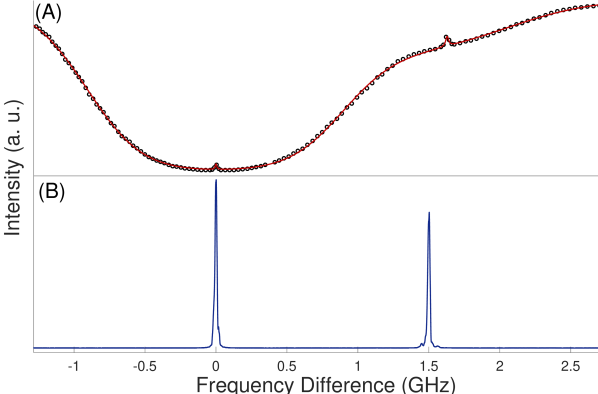
Figure 1: Wide scan of laser frequency without phase modulations or Doppler subtraction. (A) SA signal (circles), fitted with Eq. 3 (solid line). Both ${}^{20}\mathrm{Ne}$ (left) and the less abundant ${}^{22}\mathrm{Ne}$ (right) Gaussian dips, and narrow Doppler-free peaks are observed. (B) FP signal.

We implement DFS by means of saturated absorption 2013-Pressure . For a single transition with a homogeneously broadened linewidth $\Gamma$, the transmission of a weak probe beam is approximated in the Doppler limit by 1980_SA_Theory_Barium

$$\mathrm{I}[\Delta]=I_{0}e^{-\mathrm{G}[\Delta](1-S\mathrm{L}[\Delta,\Gamma])},$$ (1)

with $\mathrm{G}$ the Doppler-broadened, Gaussian absorption coefficient of the atomic vapor, including the atomic density and cell length, $S$ is the resonance depth, which depends on the pump and probe intensities, and $\Delta$ the detuning from resonance. $\mathrm{L}$ is a normalized Lorentzian transmission function $\mathrm{L}[\Delta,\Gamma]=1/(1+4(\Delta/\Gamma)^{2})$. For a sample containing two isotopes with an isotope shift of $\omega_{\mathrm{IS}}$, the transmission is given by

$$\mathrm{I}[\Delta]=I_{0}e^{-\mathrm{G}_{1}(1-S_{1}\mathrm{L}_{1})-\mathrm{G}_{2}(1-S_{2}\mathrm{L}_{2})}$$ (2)

where, assuming that the transition in both isotopes has similar linewidth, $\mathrm{L}_{2}[\Delta]=\mathrm{L}_{1}[\Delta-\omega_{\mathrm{IS}}]=\mathrm{L}[\Delta-\omega_{\mathrm{IS}},\Gamma]$, $\mathrm{G}_{2}[\Delta]=\mathrm{G}_{1}[\Delta-\omega_{\mathrm{IS}}]n_{2}/n_{1}=\mathrm{G}[\Delta-\omega_{\mathrm{IS}}]n_{2}/n_{1},$ and we suppress notation of the frequency dependencies, $n_{1},n_{2}$ are the isotopic atomic densities. We expand (2) in $\mathrm{G}_{i}S_{i}$ to get

$$\mathrm{I}[\Delta]=I_{0}e^{-\mathrm{G}_{1}-\mathrm{G}_{2}}(1+\mathrm{G}_{1}S_{1}\mathrm{L}_{1}+\mathrm{G}_{2}S_{2}\mathrm{L}_{2}+O[(\mathrm{G}_{i}S_{i})^{2}]).$$ (3)

A trace of a broad frequency scan of the SA signal (without subtraction), fitted with (3), is shown in figure 1. When the pump beam is amplitude modulated with a frequency $\omega_{\mathrm{c}}<<\Gamma$ 1971_Hansch_Lockin_pump ; 1980-FP-SA-Chooper-Rydberg , the resonance depths are modulated as: $S_{i}\rightarrow S_{i}\cos(\omega_{\mathrm{c}}t+\phi)$. Feeding the modulated signal, along with the modulation, into a lock-in amplifier, the output in-phase component becomes:

$$\mathrm{V}[\Delta]\propto\alpha_{1}\mathrm{L}_{1}+\alpha_{2}\mathrm{L}_{2}+O[(\mathrm{G}_{i}S_{i})^{3}],$$ (4)

where we evaluate the absorption coefficients on resonance: $\alpha_{1}=e^{-\mathrm{G}_{1}[0]-\mathrm{G}_{2}[-\omega_{\mathrm{IS}}]}\mathrm{G}_{1}[0]S_{1},$ and $\alpha_{2}=e^{-\mathrm{G}_{1}[\omega_{\mathrm{IS}}]-\mathrm{G}_{2}[0]}\mathrm{G}_{2}[0]S_{2}$. Equation (4) describes two Loreznians on a flat background, separated by the isotope shift, with third order nonlinear corrections to the small peak amplitudes. We now add phase modulation to the laser beam with a frequency much higher than the lock-in frequency $\omega_{\mathrm{M}}>>\omega_{\mathrm{c}}$. This creates sidebands in the pump and probe beams so that the resulting lock-in signal becomes:

$$\mathrm{V}[\Delta]\propto\\ \sum_{a=-\infty}^{\infty}{\mathrm{J}_{a}^{2}(\alpha_{1}^{a}\mathrm{L}_{1}^{a}+\alpha_{2}^{a}\mathrm{L}_{2}^{a})}+\sum_{a\neq b}{\mathrm{J}_{a}\mathrm{J}_{b}(\alpha_{1}^{ab}\mathrm{L}_{1}^{ab}+\alpha_{2}^{ab}\mathrm{L}_{2}^{ab})},$$ (5)

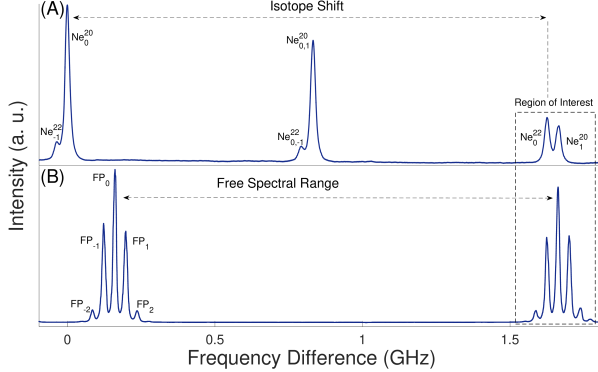
Figure 2: Wide scan of laser frequency with phase modulations. (A) SA Lock-in signal, with $\omega_{\mathrm{c}}=$$4\text{\,}\mathrm{k}\mathrm{H}\mathrm{z}$, $\omega_{\mathrm{M}}=$$1.7\text{\,}\mathrm{G}\mathrm{H}\mathrm{z}$. Ne${}^{X}_{a}$ denotes the $a$ sideband of isotope $X$. Crossovers between sidebands $a$,$a^{\prime}$ are marked Ne${}^{X}_{a,a^{\prime}}$. (B) FP signal with $\omega_{\mathrm{m}}=$$40\text{\,}\mathrm{M}\mathrm{H}\mathrm{z}$. The FSR and sidebands are denoted.

with $\mathrm{J}_{a}=\mathrm{J}_{a}[m]$ the Bessel function of order $a$ with modulation index $m$, and the sideband Lorenzians $\mathrm{L}_{i}^{a}[\Delta]=\mathrm{L}_{i}[\Delta-a\omega_{\mathrm{M}}]$. Since they are independent of the laser frequency, we do not write the expressions for the peak amplitudes $\alpha_{i}^{k}$ explicitly. The second term in (5) represents crossover peaks for each isotope obtained when the atoms are pumped by one sideband, and probed by another 2008-EOM-Crossing , $\mathrm{L}_{i}^{ab}[\Delta]=\mathrm{L}_{i}[\Delta-(a+b)\omega_{\mathrm{M}}/2]$. There are no crossover peaks between different isotopes. Figure 2 shows the measured atomic signal presented in (5). We note that crossovers either fall between, or directly add, to the original peaks.

III Frequency calibration method

In principle, it is possible to perform a wide scan similar to that presented in figure 2a and use the sideband peaks as markers for calibration of frequency axis 1997-EOM-freqcal ; however, a wide scan is more prone to frequency drifts and relies on either a completely linear scan or a complete determination of the nonlinearity 2003-Li-EOM . Instead, We scan the laser frequency only a small fraction of the actual separation, and calibrate the frequency axis using another modulated beam. When scanning the laser close to the second isotope resonance $\Delta\approx\omega_{\mathrm{IS}}$, and for a modulation frequency close to the isotope shift, $\omega_{\mathrm{M}}\approx\omega_{\mathrm{IS}}$ (region of interest in figure 2), only two peaks survive, which are separated by the difference between the modulation frequency and the isotope shift

$$\mathrm{V}[\Delta]\propto\mathrm{J}_{1}^{2}\alpha_{1}^{1}\mathrm{L}[\Delta-\omega_{\mathrm{M}}]+\mathrm{J}_{0}^{2}\alpha_{2}^{0}\mathrm{L}[\Delta-\omega_{\mathrm{IS}}].$$ (6)

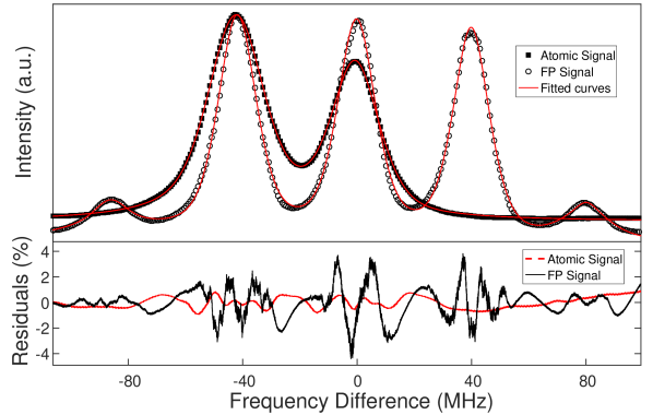
Figure 3: Narrow scan of the region of interest (see Fig. 2 for a wider scan), with typical EOM frequencies $\omega_{m}=40$ MHz and $\omega_{M}=1666$ MHz. Circle markers correspond to the atomic signal from the lock-in amplifier, fitted with (6). Full squares correspond to FP signal, fitted with (7). Residuals are quoted as percentage of signal height.

To have the remaining peaks at a similar size, we choose the appropriate modulation index ($m\approx 1)$. Generally, for a small peak with amplitude $\alpha_{2}$, and a larger one with $\alpha_{1}$, and since the modulation index can be arbitrarily small, one can always choose $m$ such that $(\mathrm{J}_{1}/\mathrm{J}_{0})^{2}\approx\alpha_{2}/\alpha_{1}$. $(\mathrm{J}_{1}/\mathrm{J}_{0})^{2}\approx(m/2)^{2}\approx\alpha_{2}/\alpha_{1}$.

To accurately calibrate the frequency axis we split another beam, modulate its phase by $\omega_{\mathrm{m}}$, and insert it into a Fabri-Pérot (FP) interferometer with finesse $F$ and FSR $\omega_{\mathrm{FSR}}$. The transmitted intensity can be written as 2010-FP-FSR-EOM

$$\mathrm{I}[\Delta]=I_{0}\sum_{a=-\infty}^{\infty}{\mathrm{J}_{a}^{2}\mathrm{L}^{a}[\Delta,\omega_{\mathrm{FSR}}/F]},$$ (7)

after filtering out terms oscillating at $a\omega_{\mathrm{m}}$ for $a\neq 0$. Equation (7) describes a series of Lorentzians, one for each sideband, separated by the modulation frequency. Figure 3 shows the Lock-in signal in the region of interest, fitted with (6), along with the frequency calibration signal, fitted with (7).

IV Implementation

Figure 4: Main elements of the experimental setup. EOM - Electro-optic modulator, HF - High frequency, LF - Low frequency, HWP - Half wave plate. FP - Fabri-Pérot interferometer, ECDL - External cavity diode laser, PBS - Polartizing beam splitter. For pressure-dependent measurements (figure…), the sealed cell was replaced by a glass tube with gas inlet (see text).

We use a narrow-band ($<$MHz) single frequency laser beam, from a home-built external cavity diode laser 2012-Steck . Frequency scanning is performed by applying voltage to a piezoelectric element connected to the external cavity grating. The beam is split in two. One part goes through a broadband, low frequency (DC-$100\text{\,}\mathrm{M}\mathrm{H}\mathrm{z}$) commercial electro-optic-modulator (EOM, New Focus 4002) and into a Fabri-Pérot cavity (Thorlabs SA-200, $\omega_{\mathrm{FSR}}=$$1.5\text{\,}\mathrm{G}\mathrm{H}\mathrm{z}$, $F=200$). The other part goes through a home-built, narrowband, high frequency EOM 1987-EOM , and enters a collinear, linearly polarized, pump-probe type setup with high-purity, natural abundance neon gas (90% ²⁰Ne, 9% ²²Ne and 0.3% ²¹Ne), contained in a AR-coated, glass cell, which resides in a high-Q coaxial resonator 1959_resonator . An RF-driven discharge at the resonance frequency ($70\text{\,}\mathrm{M}\mathrm{H}\mathrm{z}$) excites the atoms and populates higher lying states. After ignition, a few milliwatts of RF-power are sufficient to maintain stable plasma. The pump beam is amplitude modulated by a chopper at $\omega_{\mathrm{c}}=$ $4\text{\,}\mathrm{k}\mathrm{H}\mathrm{z}$. A reference beam goes through the cell as well, and provides another stage of subtraction to remove amplitude noise resulting from the laser (in part due to pointing instability and birefringent effects in the EOM) and cell discharge. The signal is fed into a lock-in amplifier (SRS SR830) where it is mixed with the chopper reference, filtered and amplified. Figure 4 shows the main elements of the experimental system.

A slow (few Hz) and narrow ($200\text{\,}\mathrm{M}\mathrm{H}\mathrm{z}$) scan of the laser frequency results in traces of the lock-in and FP signals simultaneously (figures 2 and 3). We tune the relative FP frequency position by applying DC voltage to a piezoelectric element moving one of the cavity mirrors. From (6), the distance between the zero-order ²²Ne peak and the first-order ²⁰Ne is exactly $\omega_{\mathrm{d}}=\omega_{\mathrm{M}}-\omega_{\mathrm{IS}}$. We tune the low-frequency EOM to $\omega_{\mathrm{m}}\approx\omega_{\mathrm{d}}$ by placing two of the FP sideband peaks directly on top of the lock-in atomic signal peaks (see figure 3). This limits the effects of scan nonlinearity in calibration of the frequency axis to less than a few kHz per trace. To each trace we fit the atomic signal with two Lorentzians of (6), and the FP signal with five Lorentzians corresponding to the $0,\pm 1,\pm 2$ sideband orders observed (7). To account for non-homogeneous broadening, and so model the tails of the peaks accurately, each Lorentzian in the fits is replaced with a pseudo-Voigt profile 2012_Voigt . The fitting procedure gives the distances between the FP peaks $\tau_{\mathrm{FP}}$ and the Atomic peaks $\tau_{\mathrm{LI}}$ in units of time, and so the isotope shift is calculated as:

$$\omega_{\mathrm{IS}}=\omega_{\mathrm{M}}-\omega_{\mathrm{d}}=\omega_{\mathrm{M}}-\omega_{\mathrm{m}}\frac{\tau_{\mathrm{LI}}}{\tau_{\mathrm{FP}}}.$$ (8)

This procedure of obtaining the IS is robust against frequency drifts in the laser (few MHz per minute), since both the atomic and FP signals drift together. The FP FSR is not used, and so slow (MHz per several minutes) thermal drifts in the cavity length only serve to move the FP signal relative to the atomic signal.

V Results and discussion

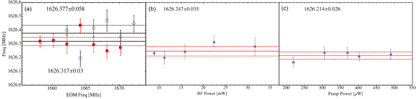
Figure 5: Calculated isotope shift frequency when varying experimental parameters, and under a constant pressure of $200\text{\,}\mathrm{m}\mathrm{T}\mathrm{o}\mathrm{r}\mathrm{r}$. Bold horizontal lines are weighted average and dashed lines represent confidence bounds of $68\%$. (a) Changing both EOM frequencies (see text). Horizontal axis labeled by the narrowband EOM frequency. Full circles are at $10$ mW RF power and empty circles are at $30$ mW. (b) Changing RF power. (c) Changing pump laser power.

For each experimental run, about $20$ traces are taken with identical parameters (laser power, pressure, etc.). The results are calculated using (8), and averaged using a Bayesian analysis approach with the Just Another Gibbs Sampler (JAGS) program 2010-andreon_scaling ; 2016-sereno_bayesian , which takes into account possible correlations between measurement errors and their intrinsic scatter.

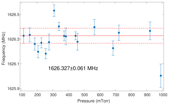
Figure 6: Calculated isotope shift frequency for varying pressure. Wighted confidence bounds to $68\%$ are indicated.

To account for unknown systematic effects we investigate the calculated IS for different experimental parameters. By varying the laser power (figure 5c), we change the width of the peaks through saturation broadening 2013-Pressure , and their height. By varying the RF-discharge power (figure 5b), we change the excited-state population and peak height, as well as shifts which may result from non-thermal distribution of the gas sample. Hysteretic effects were observed at high RF power, where coupling of the radio-waves to the plasma changed from capacitive to inductive 2015-RF_source , and so we limited our investigation to low powers. The most stringent test for our measurement scheme is to vary both EOM frequencies together (figure 5a). This changes both the distance and magnitude of all peaks involved. The above measurements were done with a sealed cell at a pressure of $200\text{\,}\mathrm{m}\mathrm{T}\mathrm{o}\mathrm{r}\mathrm{r}$. We then replaced it with a glass tube that has a gas inlet. The tube was first pumped to under one mTorr and then filled with high purity, natural abundance neon gas at various pressures. The pressure reading was stable to better than $1\%$ during an experimental run. The results of this set are presented in figure 6. Even though similar lines for ²⁰Ne are expected to shift by about $2\text{\,}\mathrm{M}\mathrm{H}\mathrm{z}\mathrm{/}\mathrm{T}\mathrm{o}\mathrm{r}\mathrm{r}$ 1996-Leo_press_neon , no pressure shift in the IS was observed within our measurement uncertainties, which indicated that the shift is similar between the isotopes to a few ten kHz per Torr.

The results of the sets presented in figure 5 and 6 are combined using the JAGS framework to obtain a wighted result of $1626.289\pm$$53\text{\,}\mathrm{M}\mathrm{H}\mathrm{z}$, where the quoted uncertainty range is one standard deviation.

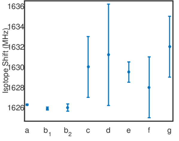
Figure 7: Isotope shift and $68\%$ confidence intervals obtained by different groups: (a) This work, (b) Feldker et. al. 2011-Birkl_IS , 1 - Absorption, 2 - Fluoresence, (c) Julien et. al. 1980-Julien , (d) Guthöhrlein et. al. 1994-Guth , (e) Basar et. al. 1997-Bassar-NeI_lines , (f) Odintsov et. al. 1965-Odinstov . (g) Konz et. al. 1992-Konz-Craft_spectroscopy .

Reference	Reported Value (MHz)	Method
This Work	$1626.287\pm 0.053$	Dual-sideband saturated absorption
2011-Birkl_IS	$1625.9\pm 0.15$	Trap absorption
2011-Birkl_IS	$1626.0\pm 0.22$	Trap fluorescence
1980-Julien	$1630\pm 3$	Velocity selective optical pumping
1994-Guth	$1631.2\pm 5.0$	Optogalvanic spectroscopy
1997-Bassar-NeI_lines	$1629.5\pm 1.0$	Intermodulated optogalvanic spectroscopy
1965-Odinstov	$1628\pm 3$	Doppler-free two-photon spectroscopy
1992-Konz-Craft_spectroscopy	$1632\pm 3$	Supersonic Beam

Table 1: Isotope shift and standard error obtained by various experimental techniques.

We now discuss the contributions of some known systematic corrections, which are not affected by the parameters scanned, to the obtained experimental value. We note here that in our measurement scheme, the ²²Ne peak appears at a lower laser frequency than the ²⁰Ne peak (See figure 2). Due to their similar electronic configuration and identical quantum numbers, most of the systematic shifts between the lines of ²⁰Ne and ²²Ne vanish to high orders when measuring the isotope shift. Among those are Zeeman shifts. The ${}^{3}\mathrm{P}_{2}$ and ${}^{3}\mathrm{D}_{3}$ levels in neon are 24 and $5\text{\,}\mathrm{T}\mathrm{H}\mathrm{z}$ away from their closest neighbours respectively. Since quantum interference shift is inversely proportional to the difference between the levels 2012-Quantum-Interf-Theory , this effect is vanishingly small in our case. Naturally, the main difference between the two isotopes is their mass $M$. It affects the atomic recoil to create the so-called recoil shift of $\omega_{\mathrm{r}}=h/(2M\lambda^{2})$, a $-2.2\text{\,}\mathrm{k}\mathrm{H}\mathrm{z}$ shift to the IS. The thermal distribution cancels first order Doppler shifts but adds a second order shift of $-4T/(\lambda c\pi M)$ 2013-Pressure , a negligible $75\text{\,}\mathrm{H}\mathrm{z}$ correction. The corrected result for the isotope shift is thus $1626.287\pm$$53\text{\,}\mathrm{M}\mathrm{H}\mathrm{z}$.

VI Conclusion

We presented a simple measurement scheme for accurate determination of intervals between far (up to few GHz) lying resonances in a spectroscopy signal. This method was used to measure the isotope shift between the ²⁰Ne and ²²Ne cooling transition with high precision. Figure 7 and table 1 shows a comparison between the results presented here, and those of other groups using various experimental techniques. We note that earlier attempts 1980-Julien ; 1994-Guth ; 1997-Bassar-NeI_lines ; 1965-Odinstov ; 1992-Konz-Craft_spectroscopy , obtain a $4\text{\,}\mathrm{M}\mathrm{H}\mathrm{z}$ larger shift than more recent and accurate ones presented in this work and in 2011-Birkl_IS . It would thus be beneficial to conduct a high accuracy, ab initio calculation of this quantity, which as far as we know, does not exist in the literature 2011-Birkl_IS .

To check our results with a different experimental system, we intend to conduct this measurement in our trap setup 2015-Our-MOT . By measuring ²¹Ne as well, it is also possible to improve determination of the ^20-22Ne charge radii difference 2008-Blaum_Ne_mass_radius .

This work was supported by the Israeli Science Foundation under ISF Grant No. (139/15); B.O. is supported by the Hoffman leadership and responsibility program, and the Eshkol Fellowship of the Ministry of Science and Technology.

References

- (1) Wieman C and Hänsch T W 1976 Phys. Rev. Lett. 36(20) 1170–1173 URL http://link.aps.org/doi/10.1103/PhysRevLett.36.1170
- (2) Inguscio M and Fallani L 2013 Atomic Physics: Precise Measurements and Ultracold Matter (OUP Oxford) ISBN 9780191509636 URL https://books.google.co.il/books?id=8zZoAgAAQBAJ
- (3) Marsman A, Horbatsch M and Hessels E 2015 Physical Review A 91 062506
- (4) Singh A K, Muanzuala L and Natarajan V 2010 Phys. Rev. A 82(4) 042504 URL http://link.aps.org/doi/10.1103/PhysRevA.82.042504
- (5) Arimondo E, Inguscio M and Violino P 1977 Rev. Mod. Phys. 49(1) 31–75 URL http://link.aps.org/doi/10.1103/RevModPhys.49.31
- (6) Hansch T W, Levenson M D and Schawlow A L 1971 Phys. Rev. Lett. 26(16) 946–949 URL http://link.aps.org/doi/10.1103/PhysRevLett.26.946
- (7) Petley B W, Morris K and Shawyer R E 1980 Journal of Physics B: Atomic and Molecular Physics 13 3099 URL http://stacks.iop.org/0022-3700/13/i=16/a=008
- (8) Walls J, Ashby R, Clarke J, Lu B and van Wijngaarden W 2003 The European Physical Journal D - Atomic, Molecular, Optical and Plasma Physics 22 159–162 ISSN 1434-6079 URL http://dx.doi.org/10.1140/epjd/e2003-00001-5
- (9) Zelevinsky T, Farkas D and Gabrielse G 2005 Phys. Rev. Lett. 95(20) 203001 URL http://link.aps.org/doi/10.1103/PhysRevLett.95.203001
- (10) Shimizu F, Shimizu K and Takuma H 1987 Japanese Journal of Applied Physics 26 L1847 URL http://stacks.iop.org/1347-4065/26/i=11A/a=L1847
- (11) Demtröder W 2013 Laser spectroscopy: basic concepts and instrumentation (Springer Science & Business Media)
- (12) Pappas P G, Burns M M, Hinshelwood D D, Feld M S and Murnick D E 1980 Phys. Rev. A 21(6) 1955–1968 URL http://link.aps.org/doi/10.1103/PhysRevA.21.1955
- (13) Pérez Galván A, Zhao Y and Orozco L A 2008 Phys. Rev. A 78(1) 012502 URL http://link.aps.org/doi/10.1103/PhysRevA.78.012502
- (14) van Wijngaarden W A and Li J 1997 Appl. Opt. 36 5905–5907 URL http://ao.osa.org/abstract.cfm?URI=ao-36-24-5905
- (15) Aketagawa M, Yashiki T, Kimura S and Banh T Q 2010 International Journal of Precision Engineering and Manufacturing 11 851–856 ISSN 2005-4602 URL http://dx.doi.org/10.1007/s12541-010-0103-3
- (16) Cook E C, Martin P J, Brown-Heft T L, Garman J C and Steck D A 2012 Review of Scientific Instruments 83 043101 URL http://scitation.aip.org/content/aip/journal/rsi/83/4/10.1063/1.3698003
- (17) Kelly J and Gallagher A 1987 Review of scientific instruments 58 563–566
- (18) Macalpine W and Schildknecht R 1959 Proceedings of the IRE 47 2099–2105
- (19) Di Rocco H and Cruzado A 2012 Acta Physica Polonica, A. 122
- (20) Andreon S and Hurn M A 2010 Monthly Notices of the Royal Astronomical Society 404 1922–1937
- (21) Sereno M 2016 Monthly Notices of the Royal Astronomical Society 455 2149–2162
- (22) Ohayon B, Wåhlin E and Ron G 2015 Journal of Instrumentation 10 P03009 URL http://stacks.iop.org/1748-0221/10/i=03/a=P03009
- (23) Leo P J, Mullamphy D F T, Peach G, Venturi V and Whittingham I B 1996 Journal of Physics B: Atomic, Molecular and Optical Physics 29 4573 URL http://stacks.iop.org/0953-4075/29/i=20/a=014
- (24) Feldker T, Schutz J, John H and Birkl G 2011 The European Physical Journal D 65 257–262 ISSN 1434-6079 URL http://dx.doi.org/10.1140/epjd/e2011-20068-5
- (25) Julien L, Pinard M and Laloe F 1980 Journal de Physique Lettres 41 479–482
- (26) Guthohrlein G and Windholz L 1994 J. Opt. Res 2 171
- (27) Basar G, Basar G, Büttgenbach S, Kröger S and Kronfeldt H D 1997 Zeitschrift für Physik D Atoms, Molecules and Clusters 39 283–289 ISSN 1431-5866 URL http://dx.doi.org/10.1007/s004600050138
- (28) Odintsov V I 1965 Optics and Spectroscopy 18 205
- (29) Konz E, Kraft T and Rubahn H G 1992 Appl. Opt. 31 4995–4997 URL http://ao.osa.org/abstract.cfm?URI=ao-31-24-4995
- (30) Marsman A, Horbatsch M and Hessels E A 2012 Phys. Rev. A 86(4) 040501 URL http://link.aps.org/doi/10.1103/PhysRevA.86.040501
- (31) Ohayon B and Ron G 2015 Review of Scientific Instruments 86 103110 URL http://scitation.aip.org/content/aip/journal/rsi/86/10/10.1063/1.4934248
- (32) Geithner W, Neff T, Audi G, Blaum K, Delahaye P, Feldmeier H, George S, Guénaut C, Herfurth F, Herlert A, Kappertz S, Keim M, Kellerbauer A, Kluge H J, Kowalska M, Lievens P, Lunney D, Marinova K, Neugart R, Schweikhard L, Wilbert S and Yazidjian C 2008 Phys. Rev. Lett. 101(25) 252502 URL http://link.aps.org/doi/10.1103/PhysRevLett.101.252502