Transformation of the frequency-modulated continuous-wave field into a train of short pulses by resonant filters

Abstract

The resonant filtering method transforming frequency modulated radiation field into a train of short pulses is proposed to apply in optical domain. Effective frequency modulation can be achieved by electro-optic modulator or by resonant frequency modulation of the filter with a narrow absorption line. Due to frequency modulation narrow-spectrum CW radiation field is seen by the resonant filter as a comb of equidistant spectral components separated by the modulation frequency. Tuning narrow-bandwidth filter in resonance with $n$-th spectral component of the comb transforms the radiation field into bunches of pulses with $n$ pulses in each bunch. The transformation is explained by the interference of the coherently scattered resonant component of the field with the whole comb. Constructive interference results in formation of pulses, while destructive interference is seen as dark windows between pulses. It is found that the optimal thickness of the resonant filter is several orders of magnitude smaller than the necessary thickness of the dispersive filters used before in optical domain to produce short pulses from the frequency modulated field.

I Introduction

Generating pedestal-free optical pulses with high peak power from a low-power laser is of great interest in optical communication Nakazawa2000 . Existing devices generally employ electro-optic amplitude modulators Harris2008 , acousto-optic modulators Warren1 ; Warren2 ; Verluise , frequency chirping followed by dispersive compensators Treacy ; Grischkowsky1974 ; Pearson ; Nakatsuka ; Nikolaus , and dispersive modulators Loy1 ; Loy2 . Application of the rapid $\pi$-phase-shift technique for CW radiation field with subsequent filtering by the optically thick resonant absorber is also capable to produce short pulses in a controllable way Chen2010 ; Macke ; Segard ; Shakhmuratov2012 ; Shakhmuratov2014 . However, this technique demands very fast phase switch, otherwise the amplitudes of the pulses reduce appreciably.

Recently, original technique for producing short pulses was reported in Vagizov ; Shakhmuratov2015 . This technique was experimentally tested with gamma photons having long coherence length (long duration of a single-photon wave packet) and the method of splitting of a single photon into pulses Vagizov ; Shakhmuratov2015 was proposed to create time-bin qubits, whose concept was introduced before in Gisin1999 ; Gisin2002 for optical photons.

The method Vagizov ; Shakhmuratov2015 is based on frequency modulation of the radiation field, which is also one of the basic elements of the frequency chirping, implemented in Grischkowsky1974 ; Pearson by electro-optic modulator. However, in spite of following dispersion compensator, which is accomplished in Grischkowsky1974 ; Pearson by near resonance absorber containing alkaline vapor, subsequent absorption (removal) of a particular spectral component is used Vagizov ; Shakhmuratov2015 . This removal method is much more flexible compared with the frequency chirping followed by a dispersive compensators Grischkowsky1974 ; Pearson and allows fine control of the duration and repetition rate of the pulses.

In this paper we analyze the capabilities of the removal method for application in optical domain and compare it with dispersion compensator method. The removal method could be implemented with cold atoms, atomic or molecular vapors, and organic molecules doped in polymer matrix. They could serve as filters to remove single frequency component of the comb spectrum produced by electro-optical modulator from CW radiation field or by modulating the resonant frequency of the filtering particles. Cold atoms possess almost naturally broadened Lorentzian absorption lines while atomic vapors at low pressure demonstrate the Doppler-broadened absorption lines. The effect of the wings of these lines on the shape of the pulses is discussed. The proposed method is capable to produce nanosecond or subnanonesocond pulses, which could be directly resolved in time by modern detectors with no use of cross-correlation technique, based on Mach-Zehnder interferometer with a delay line in one of the arms.

I have to mention also theoretical proposals to produce a train of few-cycle femto and attosecond pulses from vacuum ultraviolet or extreme ultraviolet radiation fields resonant to an atomic transition in a gas of hydrogenlike atoms, irradiated by a high-intensity low frequency (LF) laser field far detuned from all the atomic resonances. Rad10 ; Pol11 ; Antonov13 ; Antonov13PRA ; Antonov15 . These proposals consider time-dependent perturbation of the resonantly excited atomic energy level, which oscillates with the frequency of the LF laser due to Stark effect and ionization.

II Basic idea

CW radiation field $E(t)=E_{0}\exp(-i\omega_{r}t+ikz)$ after passing through the electro-optic modulator acquires phase modulation

$$E_{EO}(t)=E(t)e^{im\sin\Omega t},$$ (1)

where $\Omega$ and $m$ are the frequency and index of phase modulation. According to Jacobi-Anger expansion

$$E_{EO}(t)=E(t){\displaystyle\sum\limits_{n=-\infty}^{+\infty}}J_{n}(m)e^{im\Omega t},$$ (2)

this field is transformed into an equidistant frequency comb with spectral components $\omega_{n}=\omega_{r}-n\Omega$, where $J_{n}(m)$ is the Bessel function of the $n$-th order. Fourier transform of the field is

$$E_{EO}(\omega)=E_{0}{\displaystyle\sum\limits_{n=-\infty}^{+\infty}}J_{n}(m)\delta(\omega-\omega_{n}),$$ (3)

where $\delta(x)$ is the Dirac delta function. If CW radiation field has finite spectral width, then $\delta$ function is to be substituted by $f_{r}(\omega-\omega_{n})$ describing the spectrum of the CW field.

We transmit the frequency comb through the resonant filter with a single absorption line $F(\omega-\omega_{f})$ centered at frequency $\omega_{f}$. We select the filter whose absorption linewidth $\Gamma_{f}$ is much smaller than the distance $\Omega$ between neighboring components of the frequency comb. Such a filter is capable to remove selectively one of the spectral components of the comb. Below we don’t show explicit spatial dependence of the field amplitude hiding it into parameters of the filtered field.

By changing the carrier frequency of the CW radiation field we tune the $n$-th component of the comb $\omega_{n}=\omega_{r}-n\Omega$ close to resonance with the filter frequency $\omega_{f}$. Then the radiation field at the exit of the filter is transformed as

$$E_{fnA}(\omega)=E_{EO}(\omega)+E_{0}J_{n}(m)\left[T(\Delta_{n})-1\right]\delta(\omega-\omega_{n}),$$ (4)

where $\Delta_{n}=\omega_{n}-\omega_{f}$ and $T(\Delta_{n})$ is a transmission function of the filter, which depends on its absorption coefficient and physical thickness (see Sec. III). In general, the transmission function $T(\Delta_{n})$ is a complex function, which takes into account attenuation of the field amplitude and phase shift due to the frequency dependent refraction index (dispersion) after passing through the filter of length $L$.

For the optically thick filter at exact resonance $T(0)=T_{0}$ tends to zero. Indexes $n$ and $A$ in $E_{fnA}(\omega)$ mean that $n$-th component of the comb is in resonance with the filter and solution is approximated since in Eq. (4) we disregard the interaction of nonresonant components with the filter. Small contribution from these components due to dispersion will be taken into account in Sec. III.

Equation (4) has a simple physical meaning. It is constructed such that the first term in square brackets just describes the amplitude of the attenuated spectral component, which is in resonance and proportional to $J_{n}(m)T_{0}$. The second term removes from the comb $E_{EO}(\omega)$ the resonant component to avoid taking it into account twice. Within this approximation, other spectral components pass through the resonant filter with no change.

Inverse Fourier transformation of eq. (4) results in

$$E_{fnA}(t)=E_{0}e^{-i\omega_{r}t}\left[e^{im\sin\Omega t}+(T_{0}-1)J_{n}(m)e^{in\Omega t}\right].$$ (5)

To interpret this equation we address the argument given in Feynman lectures Feynman . According to Feynman, the light, transmitted by any sample, can be considered as a result of the interference of the input wave, as if it would propagate in vacuum, with the secondary wave radiated by the linear polarization induced in the medium. Then, following literally this argument, one can express the output field from the filter $E_{fnA}(t)$ for the input spectral comb $E_{EO}(t)$ as follows $E_{f}(t)=E_{EO}(t)+E_{sct}(t)$, where $E_{sct}(t)$ is the field, coherently scattered by the resonant atoms in the filter, whose amplitude is proportional to $(T_{0}-1)J_{n}(m)$. When filter becomes opaque for the resonant component $\omega_{n}$ (i.e., $T_{0}\rightarrow 0$), the amplitude of the coherently scattered field in the forward direction tends to the amplitude of the resonant component of the input field and their phases are opposite, i.e. $E_{sct}(t)=-E_{0}J_{n}(m)\exp(-i\omega_{n}t)$. Destructive interference of the fields results in attenuation of the $n$-th spectral component of the output field. This concept has been quantitatively proven for description of optical transients induced in the optically thick samples by fast phase switch of the incident field, which reverses destructive interference to constructive one producing short pulse whose amplitude is two times larger than the amplitude of the incident radiation field Shakhmuratov2012 .

Thus, for the frequency comb whose $n$-th spectral component interacts with the filter, just this component is coherently scattered by the atoms in the filter. The scattered field interferes with the whole frequency comb at the exit of the filter. Therefore the output radiation field reveals unusual properties.

The intensity of the field at the exit of the filter $I_{fnA}(t)=\left|E_{fnA}(t)\right|^{2}$ is described by equation

$$I_{fnA}(t)=I_{0}\left[1-2S_{n}\cos\psi_{n}(t)+S_{n}^{2}\right],$$ (6)

where $I_{0}=\left|E_{0}\right|^{2}$, $S_{n}=(1-T_{0})J_{n}(m)$ and $\psi_{n}(t)=n\Omega t-m\sin\Omega t$. If the filter is opaque for the resonant component, the amplitude of the scattered field almost coincides with the amplitude of the resonant component and $S_{n}\rightarrow J_{n}(m)$. The phases of these fields are opposite, therefore, if $\cos\psi_{n}(t)$ is positive we have destructive interference seen as a drop of intensity $I_{fnA}(t)$. If $\cos\psi_{n}(t)$ is negative, the comb and the scattered resonant component interfere constructively producing pulses. The interference becomes pronounced if $J_{n}(m)$ has global maximum. For different spectral components $n$ this maximum is achieved at different values of the modulation index $m$. We denote these values as $m_{n}$, which are $m_{1}=1.8$, $m_{2}=3.1$, $m_{3}=4.2$, … The phase difference of the comb $E_{EO}(t)$ (whose phase evolves as $m\sin\Omega t$) and the scattered field $E_{sct}(t)$ (whose phase evolves as $n\Omega t$) is $\psi_{n}(t)+\pi$ if $J_{n}(m)>0$. The evolution of $\psi_{n}(t)$ in time fully describes the formation of the pulses and the dark windows between them. Time evolution of the phase $\psi_{n}(t)$ and subsequent formation of the pulses for $n=1$, $2$, and $3$, are shown in Fig. 1 (a, b, and c, respectively).

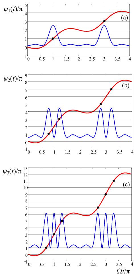
Figure 1: (color on line) Time evolution of the phase difference of the comb and resonantly scattered field component, $\psi_{n}(t)$, for $n=1$ (a), $n=2$ (b), and $n=3$ (c), thick line in red. $\pi$-pase shift is not shown in the phase difference for simplicity of notations. Black circles indicate the points when $\psi_{n}(t)=(2k+1)\pi$, where $k$ is integer. The optimal values of the modulation index are taken, i.e., $m_{1}=1.8$, $m_{2}=3.1$, and $m_{3}=4.2$ (see the text). Thin solid line in blue shows the formation of pulses according to Eq. (6). For visualization the intensity of the pulses are scaled to fit a half of each plate with no reference to the actual level of zero intensity. Numerical values of the pulse intensities and pedestal level are given in the text.

We see that the phase modulated field $E_{EO}(t)$ after passing through the resonant filter is transformed into bunches of pulses. The number of pulses in a bunch is equal to the number of filtered component of the frequency comb $n$. The intensity of the pulses is equal to $[1+S_{n}(t)]^{2}I_{0}$. For example, the maximum intensities, predicted by Eq. (6) for optimal values of the modulation index $m_{n}$ and opaque filter ($T_{0}=0$), are $I_{\max}=2.5I_{0}$ for $n=1$, $I_{\max}=2.1I_{0}$ for $n=2$, and $I_{\max}=2.06I_{0}$ for $n=3$. Thus, the intensity of the pulses exceeds almost two times the intensity of the radiation field if it would not interact with the filter. The radiation intensity between bunches is quite small because of destructive interference, which predicts $I_{\min}=[1-S_{n}(t)]^{2}I_{0}$. For the same values of the parameters $T_{0}$ and $m_{n}$ this intensity is $I_{\min}=0.175I_{0}$ for $n=1$, $I_{\min}=0.26I_{0}$ for $n=2$, and $I_{\min}=0.32I_{0}$ for $n=3$, i.e., almost an order of magnitude smaller compared with the pulse maxima.

Qualitatively the pulse bunching can be understood from the time evolution analysis of the phase $\psi_{n}(t)$. Within the period of the phase oscillation ($T_{EO}=2\pi/\Omega$), induced by electro-optical modulator, one can distinguish two intervals. Half of the period $T_{EO}/2$ the function $\psi_{n}(t)$ evolves almost linearly as $(n+m)\Omega t+C$ where $C$ is constant but different for different bunches (see Fig. 1). Within this half of the period the relation $\psi_{n}(t)=(2k+1)\pi$, where $k$ is integer, is satisfied $n$-times (shown by black circles in Fig. 1), producing pulses. During the other half of the period $T_{EO}/2$ the evolution of phase $\psi_{n}(t)$ almost stops near the value $2k\pi$, resulting in destructive interference, seen as dark windows.

III Filtering trough cold atoms

In this section we consider the frequency comb filtering through laser-cooled atoms with a modest optical depth. As an example we take parameters of ⁸⁵Rb atoms in a two-dimensional magneto-optical trap, described, for example, in Chen2010 . CW radiation field excites ⁸⁵Rb D1-line transition ($\lambda=795$ nm). Since the absorption line is almost Lorentzian, the transmission function in Eq. (4) can be described as Crisp

$$T(\Delta_{n})=\exp\left(-\frac{\alpha L\gamma/2}{\gamma-i\Delta_{n}}\right),$$ (7)

where $\alpha$ is the Beer’s law absorption coefficient, $L$ is the length of atomic cloud, and $\gamma$ is a halfwidth of absorption line. If $n$-th component of the frequency comb is in exact resonance with D1 line, then the transmission function is $T(0)=\exp(-\alpha L/2)$. Atomic cloud with a length of few millimeters demonstrates already optical depth $\alpha L=5$.

One can verify the approximate expression for the filtered field $E_{fnA}(t)$ (5) comparing it with the exact expression, which could be obtained by the convolution of $E_{EO}(t)$ field

$$E_{fn}(t)={\displaystyle\int\limits_{-\infty}^{+\infty}}E_{EO}(t-\tau)R(\tau)d\tau,$$ (8)

with the Green’s function of the absorber of thickness $L$ Shakhmuratov2012 ; Shakhmuratov2014 ; Crisp

$$R(t)=\delta(t)-\Theta(t)e^{-(i\omega_{f}+\gamma)t}j_{1}(bt)$$ (9)

where $\delta(t)$ is the Dirac $\delta$ function, $\Theta(t)$ is the Heaviside step function, $j_{1}(bt)=\sqrt{b/t}J_{1}\left(2\sqrt{bt}\right)$, $J_{1}(x)$ is the Bessel function of the first order, and $b=\alpha L\gamma/2$. For the infinitely lasting field, Eq. (8) is reduced to

$$E_{fn}(t)=E_{EO}(t)-E(t){\displaystyle\int\limits_{0}^{+\infty}}j_{1}(b\tau)e^{(i\Delta-\gamma)\tau+im\sin\Omega(t-\tau)}d\tau.$$ (10)

where $\Delta=\omega_{r}-\omega_{f}$. Index $n$ in $E_{fn}(t)$ implies that we consider the case when $n$-th spectral component of the comb is close to resonance with the filter, i.e., $\Delta=n\Omega+\Delta_{n}$ and $\Delta_{n}$ is close to zero.

Equation (10) takes into account the transformation of all spectral components of the comb including those whose change is infinitely small since they are far from resonance with the filter. Comparison of the time dependencies of the approximate intensity $I_{fnA}(t)$, Eq. (6), and exact expression $I_{fn}(t)=\left|E_{fn}(t)\right|^{2}$, where $\Delta=n\Omega$ and $\Delta_{n}=0$, is shown in Fig. 2 for $n=1$, $2$, and $3$. Optimal values of the modulation index $m=m_{n}$ are adopted in each case. The following parameters for the cold-atom filter: $\gamma/2\pi=3$ MHz, $\alpha L=5$, and $b/2\pi=7.5$ MHz, are taken. We choose the modulation frequency of the field phase equal to $30$ MHz, satisfying well the condition that $\Omega$ is much larger than the spectral width of absorption line of the filter $\Gamma_{f}=2\gamma$.

In Fig. 2(a) pulse duration from shoulder to shoulder for $n=1$ is slightly shorter than half of the period of the phase oscillation $T_{EO}/2=16.7$ ns, while duration of the dark window is slightly longer than $T_{EO}/2$ [see also Fig. 1(a)]. The pulsewidth at halfmaximum is close to but slightly shorter than $T_{EO}/4=8.3$ ns. If we have $n>1$ pulses in a bunch (see Fig. 1 and Fig. 2), their pulsewidth can be roughly estimated as $T_{EO}/4n$. Therefore, if, for example, $n=3$, the pulsewidth is already close to $1$ ns.

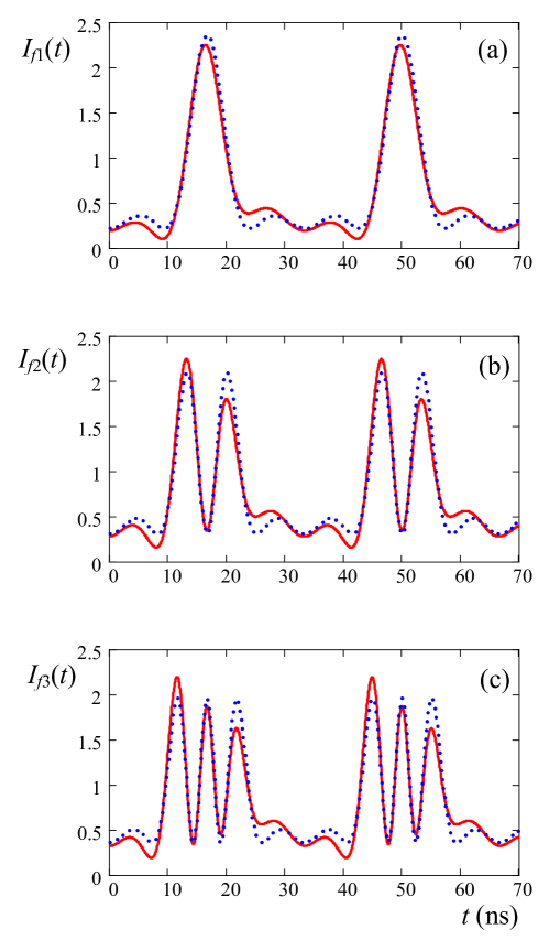
Figure 2: (color on line) Time dependence of the intensity of the filtered radiation field. Solid line in red corresponds to exact expression (10) and dotted line in blue represents the analytical approximation (6). Both are normalized to the intensity of the incident radiation field $I_{0}$. The modulation frequency $\Omega/2\pi=30$ MHz is ten times larger than the halfwidth of the absorption line of the filter $\gamma/2\pi=3$ MHz, the optical depth of the filter is $\alpha_{0}L=5$. The values of the modulation index and the number of the spectral component $n$, tuned in resonance ($\Delta_{n}=0$), are the same as in Fig. 1.

Small misfit between exact and approximate time dependencies is caused by the contribution of two nearest neighbors $\omega_{n\pm 1}=\omega_{r}-(n\pm 1)\Omega$ of the resonant spectral component $\omega_{n}$. The corrected expression, which takes them into account, is easily found

$$E_{fn}(t)\approx E_{fnA}(t)+E_{n+1}(t)+E_{n-1}(t),$$ (11)

where

$$E_{n\pm 1}(t)=E_{0}e^{-i\omega_{r}t+i(n\pm 1)\Omega t}J_{n\pm 1}(m_{n})\left(e^{\frac{-b}{\gamma-i(\Delta_{n}\mp\Omega)}}-1\right).$$ (12)

The field intensity, calculated with this correction, describes almost excellent the exact time dependence of the filtered field intensity $I_{fn}(t)$. As it is seen in Fig.2, the contribution of the sidebands introduces the asymmetry of the pulse intensities within a bunch and after-wringing, which appears in the beginning of dark windows.

Figure 3: Time dependence of the intensity of the filtered radiation field for atomic cloud of the length $L=1.5$ cm, which corresponds to the optical depth $\alpha_{0}L=33$ Chen2010 . Other parameters and notations are the same as in Fig. 2

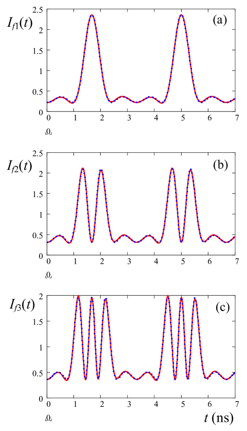
Figure 4: Comparison of the exact time dependence of the intensity of the filtered radiation field $I_{fn}(t)$ (solid line in red) with the approximate one $I_{fnA}(t)$ (blue dots) for atomic cloud with optical depth $\alpha_{0}L=5$. Modulation frequency is $\Omega/2\pi=300$ MHz. Other parameters and notations are the same as in Fig. 2

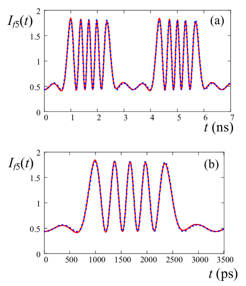
Figure 5: (a) Time evolution of intensity of the filtered radiation field for atomic cloud with optical depth $\alpha_{0}L=5$. Modulation frequency is $\Omega/2\pi=300$ MHz. The sideband $n=5$ is tuned in resonance with the filter. The value of the modulation index $m_{5}=6.4$ is close to $2\pi$. (b) Zoom in the first bunch of pules, shown in (a). Solid line in red shows $I_{fn}(t)$ and blue dots correspond to $I_{fnA}(t)$. Both are normalized to $I_{0}$.

Parameter $b=\alpha L\gamma/2$ plays a crucial role in the radiation filtering since the transmission function $T(\Delta)=\exp\left[-b/(\gamma-i\Delta)\right]$ essentially broadens if $b$ becomes larger than $\gamma$. In this case many spectral components of the comb are modified by the filter and the interference of the comb with the scattered radiation field becomes messy. Figure 3 shows a comparison of the time dependencies of exact intensity $I_{fn}(t)$ and approximate one $I_{fnA}(t)$ for atomic cloud with optical depth $\alpha L=33$, which is achieved in Chen2010 with cloud length $L=1.5$ cm. Instead of nice pulses we see their appreciable distortion. This is not surprising since for this cloud the parameter $b/2\pi=49.5$ MHz is larger than the frequency comb spacing $\Omega/2\pi=30$ MHz and many sidebands of the resonant component contribute to the pulse generating. For these values of the parameters it is necessary to take 8 neighboring components into account, i.e., four red detuned from resonance and four blue detuned. Then, the approximate expression similar to Eq. (11) but with eight additional terms $E_{n\pm k}(t)$, where $k=1$, 2, 3, and 4, gives the same result as exact equation (10). Actually the exact equation can be expressed as a result of filtering of all spectral components of the comb

$$E_{fn}(t)=E_{fnA}(t)+{\displaystyle\sum\limits_{k=1}^{\infty}}\left[E_{n+k}(t)+E_{n-k}(t)\right],$$ (13)

where

$$E_{n\pm k}(t)=E_{0}e^{-i\omega_{r}t+i(n\pm k)\Omega t}J_{n\pm k}(m_{n})\left(e^{\frac{-b}{\gamma-i(\Delta_{n}\mp k\Omega)}}-1\right).$$ (14)

Contrary to the example of the optically thick filter modifying many spectral components of the comb, we give another example when filtering becomes ideal. We take moderate optical depth $\alpha L=5$, which corresponds to $b/2\pi=7.5$ MHz, and increase modulation frequency ten times to the value $\Omega/2\pi=300$ MHz. Then, the contribution of the sidebands becomes negligible and the intensity of the filtered radiation is well described by approximate equation (6) (see Fig. 4).

It is interesting to note that the phase modulation with frequency 300 MHz is capable to produce subnanosecond pulses. Tuning, for example, the 5-th sideband of the frequency comb into resonance with the filter is capable to produce pulses with duration of 167 ps (see Fig. 5).

Cold ⁸⁵Rb atoms are not the only example of the narrow bandwidth filter. One can use also a cloud of cold potassium (³⁹K) atoms generated in a vapor-cell magneto optic trap whose excitation on the $4S_{1/2}(F=1)\leftrightarrow 4P_{1/2}(F=2)$ transition (transition wave-length 770 nm) was studied in Jeong for observation of optical precursors.

IV Filtering trough atomic vapor

In this section we consider the filtering of the frequency comb through a vapor of ⁸⁷Rb atoms and take the parameters of the experiment Lukin where spectral properties of the electromagnetically induced transparency were studied. Assume that the fundamental frequency of the comb is close to the $S_{1/2},F=1\rightarrow P_{1/2},F=2$ transition of the $D_{1}$ line of natural Rb ($\lambda=795$ nm). The atoms are confined in a cell of length $L=5$ cm. We take two temperatures of Rb vapor (50 and 70^∘C), which correspond to atomic densities $N_{1}=6\times 10^{10}$ cm^-3 and $N_{2}=6\times 10^{11}$ cm^-3, respectively. Natural linewidth of the Rb $D_{1}$ line is $\Gamma_{f}/2\pi=\gamma/\pi=5.4$ MHz and Doppler broadening is $\Delta\omega_{D}/2\pi=500$ MHz. We take the phase modulation frequency $\Omega/2\pi=10$ GHz, which is 20 times larger than the Doppler width $\Delta\omega_{D}/2\pi=500$ MHz.

The transmission function for the atomic vapor is

$$T_{D}(\Delta_{n})=\exp[-\alpha_{1,2}LF_{D}(\Delta_{n})/2],$$ (15)

where $\alpha_{1,2}=3N_{1,2}\lambda^{2}/2\pi$ is the absorption coefficient of the naturally broadened line and $F_{D}(\Delta_{n})$ is a Doppler broadened absorption line, which is

$$F_{D}(\Delta_{n})=\sqrt{\frac{\ln 2}{\pi}}\frac{2\gamma}{\Delta\omega_{D}}{\displaystyle\int\limits_{-\infty}^{+\infty}}\frac{\exp[-\ln 2(2x/\Delta\omega_{D})^{2}]}{\gamma-i(\Delta_{n}+x)}dx.$$ (16)

We have to emphasize that for both densities of Rb atoms the cell is optically thick, i.e., $\alpha_{1}L=905$ and $\alpha_{2}L=9053$. It is easy to show (see, for example, Shakhmuratov2008 ) that at exact resonance ($\Delta_{n}=0$) Eq. (16) can be approximated as

$$F_{D}(0)=\sqrt{\pi\ln 2}\frac{2\gamma}{\Delta\omega_{D}}.$$ (17)

Therefore for $\Delta_{n}=0$ the effective optical depth, $\alpha_{1,2}LF_{D}(0)$, is reduced almost hundred times since the Doppler width $\Delta\omega_{D}$ is two orders of magnitude larger than the natural linewidth $2\gamma$.

If $\left|\Delta_{n}\right|>1.8\Delta\omega_{D}$, then the absorption line reveals Lorenzian wings (see, for example, Fig. 1 in Ref. Shakhmuratov2008 ), which can be approximated as

$$F_{D}(\Delta_{n})=\frac{\gamma}{\gamma-i\Delta_{n}}.$$ (18)

Therefore, the contribution of far wings of the dispersion $\chi^{\prime}(\Delta_{n\pm k})\sim\operatorname{Im}F_{D}(\Delta_{n\pm k})$ in the filtering of nonresonant components $\omega_{r}-(n\pm k)\Omega$ of the frequency comb could be noticeable if $\Delta_{n}=0$. For example, the contribution of the nearest sidebands ($k=\pm 1$) of the resonant component is proportional to

$$E_{n\pm 1}(t)\sim J_{n\pm 1}(m_{n})\left(e^{\mp ib_{1,2}/\Omega}-1\right),$$ (19)

where $b_{1,2}=\alpha_{1,2}\gamma/2$. For the atomic density $N_{1}$ the ratio $b_{1}/\Omega=0.122$ is small since $b_{1}/2\pi=1.2$ GHz and modification of the sidebands due to filtering does not influence significantly the shape of the produced pulses. For the atomic density $N_{2}$ the ratio $b_{2}/\Omega=1.22$ is large since $b_{2}/2\pi=12$ GHz and the sidebands change their phases due to filtering. In this case one can expect appreciable corruption of the produced pulses. To verify these expectations we calculate the intensity of the filtered comb taking into account the modification of many sidebands. The number of them can be limited by $\pm k_{\max}$ if the contribution of the next sidebands $\pm(k_{\max}+1)$ does not change the signal.

Substituting the transmission function $T_{D}(\Delta_{n})$ into equations (5) and (14) one obtains the modified Eq. (13), which describes the transformation of the frequency comb after passing through the atomic-vapor filter. The substitution changes the functions $S_{n}$ and $E_{n\pm k}(t)$ to

$$S_{n}=J_{n}(m_{n})[1-T_{D}(0)],$$ (20)

$$E_{n\pm k}(t)=E_{0}e^{-i\omega_{r}t+i(n\pm k)\Omega t}J_{n\pm k}(m_{n})\left[T_{D}(\mp k\Omega)-1\right],$$ (21)

where $\Delta_{n}=0$, which implies that the $n$-th spectral component is in exact resonance with the filter.

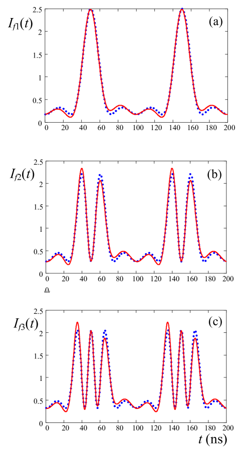
Figure 6: Time dependence of the intensity of the filtered radiation field $I_{fn}(t)$ (solid line in red) for atomic vapor with optical depth $\alpha_{1}L=905$. Modulation frequency is $\Omega/2\pi/2\pi=10$ GHz. The approximate time dependence of the intensity $I_{fnA}(t)$ is shown by blue dots. Other parameters and notations are the same as in Fig. 2

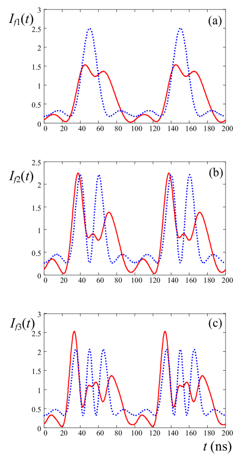
Figure 7: Time dependence of intensity of the radiation field filtered through the atomic vapor with the optical depth $\alpha_{2}L=9053$ (solid line in red). Other parameters and notations are the same as in Fig. 6

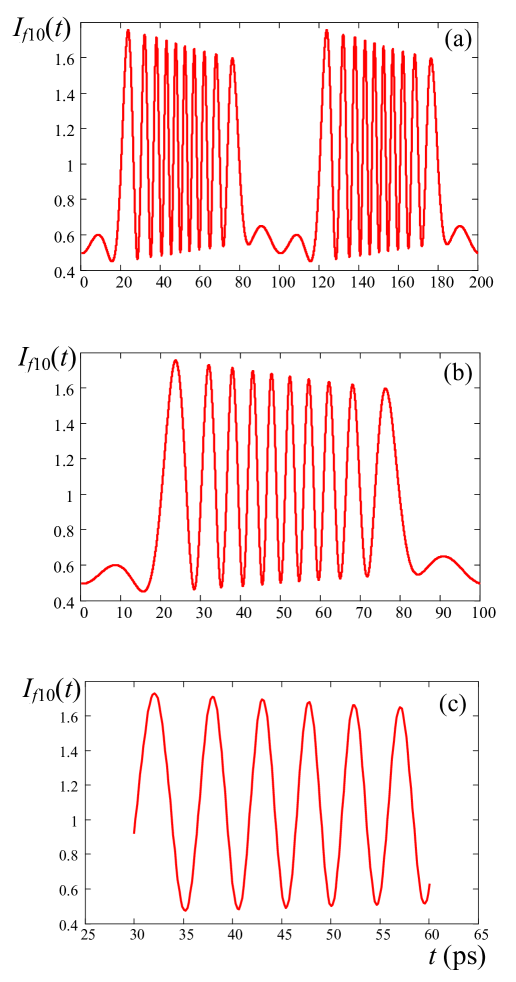
Figure 8: (a) Time dependence of intensity of the radiation field filtered through the atomic vapor with the optical depth $\alpha_{0}L=453$. The spectral component $n=10$ is tuned in resonance with the filter and the phase modulation index is $m_{10}=11.8$. (b) The content of a bunch of pulses. (c) Zoom in a central part of the bunch. Other parameters and notations are the same as in Fig. 6

For the Rb cell with atomic density $N_{1}=6\times 10^{10}$ cm^-3 it is enough to take into account the contribution of two spectral components ($n\pm 1$) neighboring the resonant component $n$. For this density the effective optical depth of the cell at the absorption line center is $\alpha_{1}LF_{D}(0)=14.4$. The result of the comb filtering through the cell is shown in Fig. 6. If $n=1$, $2$, or $3$ spectral component is in resonance with the filter, the pulses with the width 25, 12.5, and 8.3 ps, respectively, are produced.

If atomic density is increased by the order of magnitude to $N_{2}=6\times 10^{11}$ cm^-3, then eight sidebands of the resonant component $n\pm 1$, $n\pm 2$, $n\pm 3$, and $n\pm 4$ give noticeable contribution. Therefore, the intensity modulation of the filtered comb becomes messy (see Fig. 7). Actually, for $n=2$ and $n=3$ it is necessary to take into account the contribution of 14 sidebands (up to $n\pm 7$).

To obtain nice and clean pulses it is preferable to use a filter with a smaller optical depth. An example of filtering by a cell with optical depth $\alpha L=453$ the spectral component $n=10$ of the frequency comb, produced by phase modulation with the optimal value of the modulation index $m_{10}=11.8$ (which is close to $2\pi$), is shown in Fig. 8. Such a filtering is capable to produce pulses as short as $2.5$ ps, which are grouped in bunches consisting of 10 pulses. Thus, by phase modulation technique and subsequent filtering it is possible to create pulses whose duration is 40 times shorter than the modulation period.

V Femtosecond pulses

It is also possible to create femtosecond pulses if high order harmonic of the frequency comb is removed. For simplicity we consider an ensemble of two-level atoms, for example, a vapor of alkaline atoms. We take the modulation frequency of the radiation field equal to $\Omega/2\pi=10$ GHz. If the modulation index is $m_{100}=104$, the amplitude of the frequency component $\omega_{r}-100\Omega$ takes its first maximum value, which is proportional to $J_{100}(104)=0.144$. Removal of this spectral component of the comb by atomic filter leads to high frequency oscillations of the transmitted field intensity. Duration of the pulses is estimated as $T_{EO}/400=250$ fs, where $T_{EO}$ is the phase modulation period. The necessary modulation index $m_{100}=104$ corresponds to a voltage, which is $33$ times larger than the have-wave voltage of electro-optical modulator. One can expect to reach this value by increasing the voltage and/or the physical length of the modulator by an order of magnitude.

Below the simplified picture of the filtering of high order harmonics of the frequency comb is illustrated. To avoid complicated expressions, we approximate the coherently scattered component of the field in Eq. (6) as proportional to $S_{100}=J_{100}(m_{100})$, assuming that the resonant absorption is close to $100\%$, i.e., $T_{D}(0)\approx 0$. We disregard the dispersive contribution of the neighboring spectral components. Time dependence of the intensity of the filtered radiation field is shown in Fig. 9 (a and c). The contrast of the pulses is not as large as for filtering of low order harmonics. This is because the intensity of the maxima and minima of the pulses can be estimated as $I_{\max}\approx[1+2J_{100}(104)]I_{0}$ and $I_{\min}\approx[1-2J_{100}(104)]I_{0}$. Since $J_{100}(104)=0.144$, the maxima exceeds $30\%$ the level of the intensity of the incident radiation field, while minima are smaller than $I_{0}$ on $30\%$ of its value.

The amplitudes of high harmonics of the frequency comb decrease with increase of their number $n$ since the first maxima of the Bessel functions $J_{n}(m_{n})$ decrease with increase of the order $n.$ To achieve large contrast of the pulses, one can remove several spectral components of the comb neighboring $n=100$, if they have the same phase at time of the pulse formation. As an example we consider the case if filtering of the comb component $n=100$ is accompanied by filtering of the components with the numbers $n+2k$, where $k$ takes values $\pm 1$ and $\pm 2$. These spectral components have the same phase as $n=100$ spectral component at times when central pulses of the bunch are formed. The amplitude of the filtered radiation filed with cumulative contribution of extra four spectral components of the comb due to their removal by separate filters is approximated as

$$E_{cum}(t)=E(t)\left[e^{im\sin\Omega}-\sum_{k=-2}^{2}J_{n+2k}(m)e^{i(n+2k)\Omega t}\right],$$ (22)

where, for simplicity, it is supposed that $T_{D}(0)=0$. The intensity of the filtered radiation field $I_{cum}(t)=\left|E_{cum}(t)\right|^{2}$ is shown in Fig. 9 (b and c). The central part of the pulse bunches demonstrates good contrast. The maximum accumulative effect of five spectral components is achieved if $m=103$.

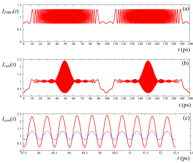
Figure 9: (a) Time dependence of the intensity of the radiation field whose $n=100$ spectral component is removed by the filter. The modulation frequency is $\Omega/2\pi=10$ GHz. (b) Accumulative result of the filtering of the additional four spectral components of the frequency comb (see the text for details). (c) Zoom in a central part of the bunch. Accumulative effect is shown by solid line (in read), while dotted line (in blue) demonstrates the result of the filtering of only one spectral component with $n=100$. Full width at half-maximum of the pulses is close to $250$ fs as it is expected from simple estimations.

Cumulative filtering is possible if we have narrow bandwidth filters properly adjusted for chosen spectral components of the frequency comb. By a set of cells with atomic vapors it is hard to construct such a specific multifrequency filter having a large spacing between the absorptive frequency components of the order of $20$ GHz. However, for example, cesium atoms have a large hyperfine splitting of the ground state seen as a spectral doublet with a spacing equal to $9.2$ GHz. If we reduce the modulation frequency of the field phase down to $\Omega/2\pi=4.6$ GHz, populate properly ground state levels by pumping Cs atoms such that both components of the doublet are strongly absorptive, then we could remove two spectral components of the frequency comb. An example of cumulative filtering of two spectral components $100\Omega$ and $98\Omega$ by cesium atoms is shown in Fig. 10 (b and c). The increase of the intensity of the pulses is clearly seen. Since the modulation frequency is decreased by a factor of two, the duration of pulses increases by the same factor to $500$ fs.

Cumulative filtering of two spectral components by atoms with the spectral doublet produces pulses with modest contrast. The ratio of the maxima of the pulse intensities to their minima is close to three. To make pulse minima close to zero one can use destructive interference of the filtered radiation field $E_{cum}(t)$ with the field $E_{EO}(t)$ from the same electro-optic modulator but with the opposite phase and reduced amplitude, i.e.,

$$E_{rdc}(t)=E_{cum}(t)-RE_{EO}(t),$$ (23)

where $R$ is the amplitude reduction factor. For the case of the filtering with the doublet the reduction factor is $R=1-J_{100}(103)-J_{98}(103)$. Then, due the interference the pulse minima at the bunch center become zero, while the amplitude of the pulse maxima reduces to the value $2[J_{100}(103)-J_{98}(103)]E_{0}=0.55E_{0}$. The result of this interference is shown in Fig. 10 (d and e) for the field intensity $I_{rdc}=\left|E_{rdc}(t)\right|^{2}$.

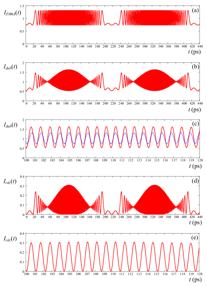
Figure 10: (a) Time dependence of the intensity of the radiation field whose $n=100$ spectral component is removed by the filter. The modulation frequency is $\Omega/2\pi=4.6$ GHz and modulation index is $m_{100}=104$. (b) Accumulative result of the filtering of the additional spectral component $n=98$ of the frequency comb by the doublet (see the text for details). The modulation index is $m=103$. (c) Zoom in a central part of the bunch. Accumulative effect is shown by solid line (in read), while dotted line (in blue) demonstrates the result of the filtering of only one spectral component with $n=100$. Full width at half-maximum of the pulses is close to $500$ fs as it expected from simple estimations. (d) The result of the filtering with the doublet, followed by reduction of the field amplitude due to the destructive interference with the reduced field from electro-optic modulator whose phase is shifted by $\pi$. (e) Zoom in the central part of the pulse bunch, shown in (d).

Cumulative filtering is better to implement by organic molecules doped in polymer matrix, which undergo persistent spectral hole burning at liquid helium temperature. In such a filter the frequency resolution is limited by the width of the homogeneous zero-phonon lines of the chromophore molecules. For example, waveguide narrowband optical filter, which consists a planar waveguide with a thin polymer film containing molecules, which undergo persistent spectral hole burning at liquid helium temperature, demonstrates transmission bandwidth less than 1 GHz Tschanz1995 ; Tschanz1996 . Saturated holes are burned in waveguide geometry by illumination in the transverse direction with low absorption, whereas the probing is carried out in longitudinal wave guiding directions with high absorption. The waveguide with spectral hole burning can act as integrated sub-gigahertz narrow-band filter, which is proposed to observe slow light phenomenon Shakhmuratov2005 ; Rebane2007 .

Comb structures of arbitrary shapes in transmission spectra were created experimentally in organic molecules doped in a polymer Rebane1995 ; Wild2002 . Therefore, one can expect that it is experimentally possible to create a broad hole with, say, five absorptive peaks in it. For cumulative filtering it is enough to create a broad hole with the width $\sim 10$ cm^-1 and five absorptive peaks in it with $20$ GHz spacing and widths less than $1$ GHz.

VI Coherent Raman scattering with resonant filtering

Frequency modulation (FM) of the field, followed by a dispersive compensator to produce short pulses, could be substituted by dispersive modulators Loy1 ; Loy2 ; Grischkowsky1975 . In dispersive modulators, where instead of modulating the frequency of the light, the resonant frequency of the filter is modulated. Both techniques, FM followed by dispersive compensator and dispersive modulator, use light-matter interaction, which results in a phase change of the field spectral components, being far from resonance. Here I propose to make a specific resonant filtering in the interaction process of light with particles whose resonant frequencies experience modulation. Theoretical description of this process is very similar to that, proposed in Grischkowsky1975 . The only difference is the resonant condition imposed on one spectral component.

In the linear response approximation the propagation of the CW radiation field $E(z,t)=E_{0}\exp(-i\omega_{r}t+ikz)$ through the resonant medium is described by the set of equations

$$\widehat{L}\chi(z,t)=i\alpha\gamma\sigma_{eg}(z,t)/2,$$ (24)

$$\dot{\sigma}_{eg}=(i\Delta-\gamma)\sigma_{eg}+i\chi(z,t),$$ (25)

where $\widehat{L}=\partial_{z}+c^{-1}d_{t}$, $\chi(z,t)=d_{eg}E_{0}(z,t)/2\hbar$ is the Rabi frequency of the field proportional to the slowly varying field amplitude $E_{0}(z,t)=E(z,t)\exp(i\omega_{r}t-ikz)$, which satisfies the boundary condition $E_{0}(0,t)=E_{0}$ at the entrance to the medium with coordinate $z=0$; $d_{eg}$ is a matrix element of the dipole transition between ground, $g$, and excited, $e$, states of a molecule (NH₃ in the experiment of Loy Loy1 ); $\rho_{eg}=\sigma_{eg}\exp(-i\omega_{r}t+ikz)$ is the nondiagonal element of the molecular density matrix and $\sigma_{eg}$ its slowly varying part; $\gamma$ is the decay rate of the coherence of the states $e$ and $g$, $\Delta=\omega_{r}-\omega_{0}$ is the detuning from the resonant frequency $\omega_{0}$ of molecules, and $\alpha$ is the resonant absorption coefficient of the molecular vapor.

The resonant frequency of molecules is externally controlled via the Stark effect. Long Stark sell, with a small plate separation, is a parallel-plate transmission line. A bias electric filed is used to control the dc frequency separation between the input light and the relevant molecular transition. An applied rf voltage travels in the same direction as the light. Therefore, the resonant detuning is $\Delta=\Delta_{b}+\Delta_{rf}\cos\Omega t$, where $\Delta_{b}$ is the dc offset between the radiation frequency and the absorption line center due to the bias voltage, $\Omega$ is the rf voltage frequency, and $\Delta_{rf}$ is the amplitude of the time-dependent frequency modulation.

For this parallel plate transmission line the Stark voltage travels at $c$ to a very good approximation. Therefore spatiotemporal dependence of $\Delta$ satisfies the equation

$$\widehat{L}\Delta(z,t)=0,$$ (26)

whose solution is $\Delta(z,t)=\Delta(t-z/c)$.

With the help of new variables

$$\chi_{comb}(z,t)=\chi(z,t)e^{im\sin\Omega t^{\prime}},$$ (27)

$$p_{eg}(z,t)=\sigma_{eg}(z,t)e^{im\sin\Omega t^{\prime}},$$ (28)

equations (24) and (25) are reduced to

$$\widehat{L}\chi_{comb}(z,t)=i\alpha\gamma p_{eg}(z,t)/2,$$ (29)

$$\dot{p}_{eg}=(i\Delta_{b}-\gamma)p_{eg}+i\chi_{comb}(z,t),$$ (30)

where $t^{\prime}=t-z/c$ is the local time and $m=\Delta_{rf}/\Omega$.

There are no time dependent coefficients in these equation. Therefore, their steady state solution can be found in the form

$$\chi_{comb}(z,t)={\displaystyle\sum\limits_{n=-\infty}^{+\infty}}\chi_{n}(z)e^{in\Omega t^{\prime}},$$ (31)

$$p_{eg}(z,t)={\displaystyle\sum\limits_{n=-\infty}^{+\infty}}p_{n}(z)e^{in\Omega t^{\prime}},$$ (32)

where

$$p_{n}(z)=\frac{-\chi_{n}(z)}{\Delta_{b}-n\Omega+i\gamma},$$ (33)

$$\chi_{n}(z)=T_{n}(z)\chi_{n}(0),$$ (34)

$$T_{n}(z)=\exp\left[\frac{-\alpha z/2}{1-i(\Delta_{b}-n\Omega)/\gamma}\right],$$ (35)

$\chi_{n}(0)=\chi(0)J_{n}(m)$, and $\chi(0)=d_{eg}E_{0}/2\hbar$.

For a Doppler-broadened line, whose homogeneous linewidth $2\gamma$ is much smaller than the Doppler width $\Delta\omega_{D}$, the transmission function $T_{n}(z)$ is modified as in Sec. IV [see Eqs. (15), (16)].

In Loy’s experiments Doppler width $\Delta\omega_{D}/2\pi=87$ MHz was larger than rf modulation frequency $\Omega$, which varied between $30$ and $50$ MHz. The dc offset $\Delta_{b}$ was comparable or much larger than $\Delta\omega_{D}$. Therefore, the spectral components of the frequency comb $\chi_{comb}(z,t)$ mainly acquired different phase shifts at the exit of the dispersive filter. This is the core idea of the dispersive modulators.

We propose to employ modulation frequency, which is much larger than Doppler width (for example, $\Omega/2\pi=300$ MHz, which is almost an order of magnitude larger than $\Delta\omega_{D}/2$). Then, if one of the spectral components of the comb $\chi_{comb}(z,t)$ comes to resonance with molecular vapor, pulse bunches are developed at the exit of the modulating filter similar to those shown in Fig. 4.

The physical origin of the pulse formation in our case can be explained as follows. If all spectral components of the comb are far from resonance with the vapor, one can neglect their change assuming that $\chi_{n}(z)\approx\chi_{n}(0)$. Then, we have

$$\chi_{comb}(z,t)=\chi(0){\displaystyle\sum\limits_{n=-\infty}^{+\infty}}J_{n}(m)e^{in\Omega t^{\prime}}=\chi(0)e^{im\sin\Omega t^{\prime}}.$$ (36)

Applying transformation inverse to (27), we obtain no change of the radiation field at the exit of the filter, i.e., $\chi(z,t)=\chi(0,t^{\prime})$.

If $n$-th spectral component of the comb is removed by the filter, then the comb changes as

$$\chi_{comb}(z,t)=\chi(0)\left[e^{im\sin\Omega t^{\prime}}-J_{n}(m)e^{in\Omega t^{\prime}}\right].$$ (37)

In the laboratory reference frame (after the inverse transformation) we obtain

$$\chi(z,t)=\chi(0)\left[1-J_{n}(m)e^{in\Omega t^{\prime}-im\sin\Omega t^{\prime}}\right].$$ (38)

Constructive interference of the time dependent component with the constant one results in formation of pulses, while their destructive interference gives dark windows. This equation can be interpreted as a resonant interaction of the $n$-th component with molecules followed by Raman rescattering in all the sidebands. In this picture the primary source of the radiation field is the polarization excited by resonant component $\chi(0)J_{n}(m)\exp(in\Omega t^{\prime})$. This excitation is rescattered coherently into $\chi(0)J_{n}(m)J_{k}(m)\exp[i(n-k)\Omega t^{\prime}]$ components (with $k$ varied from $+\infty$ to $-\infty$) due to the modulation of the resonant frequency of the molecules.

VII Discussion

FM followed by dispersive compensator scheme for producing optical pulses have been based on the ideas of chirp radar Klauder1960 ; Duguay1966 ; Duguay1968 . In the chirp radar system the transmitted pulse is of relatively long duration $\Delta t$ during which time the instantaneous frequency is swept over the range $\omega\rightarrow\omega+\Delta_{chirp}$ satisfying the condition $\Delta_{chirp}\Delta t\gg 1$. The return pulse is passed through a dispersive network providing a differential delay $\Delta t$ over the frequency range $\Delta_{chirp}$. As a result, the energy at the beginning of the pulse is delayed so as to reach the end of the network at the same time as the energy at the end of the pulse. The duration of the compressed pulse produced this way is of the order of $\delta t\approx 1/\Delta_{chirp}\ll\Delta t$.

In optical domain electrooptical modulation of the radiation frequency Grischkowsky1974 spreads its spectrum over the range $m\Omega$. In Loy’s dispersive filter rf voltage due to Stark effect spreads effectively the field spectrum over the range $\Delta_{rf}=m\Omega$. In both schemes dispersive properties of atoms or molecules are used to have frequency-dispersive group velocities of the spectral components produced by modulation. Therefore, both schemes require resonant media with a very large optical thickness and employ large offset between the radiation frequency and the absorption line center to avoid the absorptive losses. These constrains force to work with relatively small frequencies $\Omega$ and large modulation index $m$. Then, many spectral components of the comb acquire appreciable dispersive phase shifts with large difference between blue and red borders of the comb spectrum.

It is quite easy to estimate parameters of the dispersive filter, which is capable to compress phase modulated field into short pulses within the chirp radar model. We take as an example the parameters used in the experiment of Pearson et al. Pearson who compressed phase modulated CW radiation field by passing it trough a sodium vapor. Resonant detuning $\Delta_{c}/2\pi=(\omega_{r}-\omega_{f})/2\pi=4$ GHz was large compared with the phase modulation frequency $\Omega/2\pi=200$ MHz. The modulation index $m\approx 2\pi$ was moderate.

If the field phase is modulated according to $\varphi(t)=m\sin\Omega t$, then the effective resonant detuning evolves in time as $\Delta(t)=\Delta_{c}-m\Omega\cos\Omega t$. Half a period this detuning increases taking maximum value $\Delta_{\max}/2\pi=(\Delta_{c}+m\Omega)/2\pi=5.26$ GHz at $t_{\max}=(2n+1)\pi/\Omega$, another half it decreases taking minimum value $\Delta_{\min}/2\pi=(\Delta_{c}-m\Omega)/2\pi=2.74$ GHz at $t_{\min}=(2n+2)\pi/\Omega$, where $n$ is an arbitrary integer number. Portion of radiation field with frequencies detuned from resonance by $\Delta_{\max}$ travels through the vapor cell with group velocity larger than that portion, which is detuned by $\Delta_{\min}$. If the latter is produced at earlier time, for example, at $t_{\min}=2n\pi/\Omega$, and the former at later time, for example, at $t_{\max}=(2n+1)\pi/\Omega$, they have a chance to arrive at the exit of the cell at the same time if the difference of their group velocities is appropriate. The same is true for all the intermediate spectral components of the field. Such a compression of spectral components of the field happens between $t_{\min}=2n\pi/\Omega$ and $t_{\max}=(2n+1)\pi/\Omega$. In the next half a period of phase modulation, between $t_{\max}=(2n+1)\pi/\Omega$ and $t_{\min}=(2n+2)\pi/\Omega$, these spectral components are spread since the late component comes much later than the first component. In this half a period the difference of the group velocities of the spectral components of the field results in a drop of the radiation intensity.

Delay time of the spectral components can be estimated as $\tau_{d}=\alpha L\gamma/2\Delta^{2}$, where $\Delta$ is the resonant detuning of the spectral component Shakhmuratov2008 . Then, we have for two spectral components $\Delta_{\min}$ and $\Delta_{\max}$ two delay times $\tau_{d\min}$ and $\tau_{d\max}$. To observe the pulse compression we need to satisfy the condition $\tau_{d\min}-\tau_{d\max}=T_{EO}/2$, where $T_{EO}=2\pi/\Omega$ is a phase modulation period. In the experiment Pearson this condition is $\tau_{d\min}-\tau_{d\max}=2.5$ ns. It is realized if $\alpha L=6.5\times 10^{4}$.

To verify these estimations we use simplified expression for the filtered field amplitude

$$E_{f}(t)=E(t){\displaystyle\sum\limits_{n=-\infty}^{+\infty}}J_{n}(m)e^{in\Omega t-\frac{\alpha L\gamma/2}{\gamma-i(\Delta_{c}-n\Omega)}},$$ (39)

where $\gamma$ is the homogeneous dephasing rate ($\gamma/2\pi=5$ MHz). Here we disregard the Doppler broadening because of large detuning $\Delta_{c}$ (see the arguments in Sec. IV).

Time dependence of the intensity of the filtered radiation field $I_{f}(t)=\left|E_{f}(t)\right|^{2}$, which is described by Eq. (39), is shown in Fig. 11 (solid lines in red) for the parameters specified above. The pulses look quite similar to those shown in Fig. 2(b) in Ref. Pearson . Time dependence of the intensity for $\alpha L$ two times smaller than the optimal value, Fig. 11(a), and two times larger, Fig. 11 (b) are shown by dotted lines (in blue) for comparison.

It is instructive to express the field amplitude $E_{f}(t)$, taking into account finite number of terms of the absorption line Taylor series

$$\frac{\alpha L\gamma/2}{\gamma-i(\Delta_{c}-n\Omega)}\approx i\frac{\alpha L\gamma}{2\Delta_{c}}\left(1+\frac{n\Omega}{\Delta_{c}}+\frac{n^{2}\Omega^{2}}{\Delta_{c}^{2}}+\frac{n^{3}\Omega^{3}}{\Delta_{c}^{3}}+...\right),$$ (40)

where the contribution of the coherence decay rate $\gamma$ in the denominator is disregarded since $\gamma\ll\Delta_{c}$. The first term of this series describes the constant phase shift of the field. The second term reduces the group velocity of the pulsed field. The third and fourth terms result in dispersion and higher order dispersion of the group velocities of the spectral components of the pulse.

If we take into account only three terms of the series, then for the specified values of the parameters Eq. (39) is reduced to

$$E_{d}(t)=E(t)e^{i\varphi_{d}}{\displaystyle\sum\limits_{n=-\infty}^{+\infty}}J_{n}(m)e^{in\left(\Omega t-a-\varepsilon_{1}n\right)},$$ (41)

where $\varphi_{d}=-\alpha L\gamma/2\Delta_{c}$, $a=2.03$, and $\varepsilon_{1}=0.102$. Time dependence of the intensity $I_{d}(t)=\left|E_{d}(t)\right|$, where only first three terms of the series are taken into account including dispersion of the group velocities, is shown in Fig. 11(c) by dotted line (in blue). Group velocity dispersion of the spectral components of the phase modulated field in a dispersive filter results in a compression of the field into a single pulse of short duration with two small side lobes.

If we take into account also the contribution of the fourth term in the series (40), which produces dispersion of the group velocity dispersion, then Eq. (39) is reduced to

$$E_{dd}(t)=E(t)e^{i\varphi_{d}}{\displaystyle\sum\limits_{n=-\infty}^{+\infty}}J_{n}(m)e^{in\left(\Omega t-a-\varepsilon_{1}n-\varepsilon_{2}n^{2}\right)},$$ (42)

where $\varepsilon_{2}=0.005$. Time dependence of the intensity $I_{dd}(t)=\left|E_{dd}(t)\right|$ is shown in Fig. 11(d) by dotted line (in blue). The forth term results in a pulse ringing and reduction of the pulse intensity.

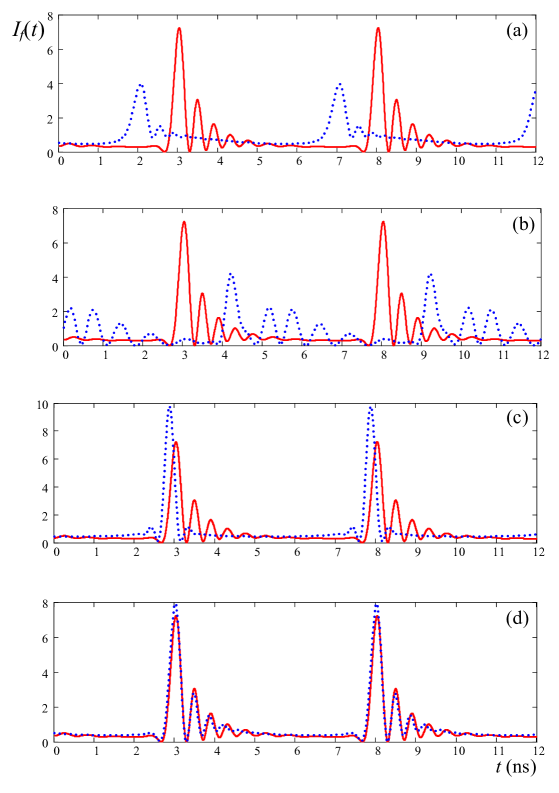
Figure 11: Time dependence of the intensity of the radiation field filtered through a dispersive filter with different group velocities of the spectral components of the phase modulated field, solid line (in red). Dotted line (in blue) shows the same dependence but for the filter, which is two times shorter (a), longer (b). Time dependence of the intensity (dotted line in blue) if we disregard (c) or take into account (d) the forth term of Taylor series of the absorption line, which is responsible for higher order dispersion of the group velocity of spectral packets.

According to the numerical analysis the first pulse, shown by dotted line (in blue) in Fig. 11(c), takes its maximum value at $t_{p}$ when $\Omega t_{p}-a=\pi/2$. Intuitively, this is consistent with the concept of the chirp radar model. Time delay $t_{c}$ of the fundamental frequency component $\omega_{r}$ ($n=0$) at the exit of the dispersive filter satisfies the condition $\Omega t_{c}-a=0$ since the parameter $a$ is calculated for the detuning $\Delta_{c}$, while the most detuned spectral component $\Delta_{c}+m\Omega$ appears quarter of the period $T_{EO}$ later. Therefore, pulse compression takes place when $\Omega t_{p}-a=\pi/2$. Individual phase shifts of the spectral components $\omega_{r}-n\Omega$ with $n\neq 0$ due to dispersion of their group velocities are described by the term $in^{2}\varepsilon_{1}$ in the exponent in Eq. (41).

At time $t_{p}$ the field amplitude takes the value

$$E_{d}(t_{p})=E(t_{p})e^{i\varphi_{d}}{\displaystyle\sum\limits_{n=-\infty}^{+\infty}}i^{n}J_{n}(m)e^{-i\varepsilon_{1}n^{2}},$$ (43)

where $i^{n}=\exp(in\pi/2)$. Numerical calculation of the sum in Eq. (43) gives

$${\displaystyle\sum\limits_{n=-\infty}^{+\infty}}i^{n}J_{n}(m)e^{-i\varepsilon_{1}n^{2}}=2.22-2.26i,$$ (44)

and $I_{d}(t_{p})=9.62I_{0}$.

In the scheme of resonant filtering, proposed in the presented paper, only one spectral component of the comb is removed by a resonant absorber. Optical thickness of the absorber is to be modest to avoid phase change of nonresonant components of the comb. Then, short pulses are produced. Their duration is close to $\pi/2n\Omega$, which qualitatively differs from the pulse duration in the dispersive compensator scheme, estimated according to the chirp radar as $1/2m\Omega$. Quantitatively these durations are also different since the optimal values of the modulation index in our scheme can be roughly estimated as $m\approx\pi n/2$ for $n=\pm 1,\pm 2,\pm 3$ and $m\approx n$ for large $n$. A specific qualitative difference of the schemes is that the modulation frequency in our scheme is to be large, at least much larger than the width of the absorption line of the resonant filter. The modulation index $m$ is also must be large to make pulses as short as possible. However, if the modulation index exceeds $20$, several spectral components should be removed to keep large contrast of the produced pulses. These components have to be spaced apart from the target component $\omega-n\Omega$ by $\pm 2\Omega$, i.e. the accompanying spectral components to be removed are $\omega-(n\pm 2)\Omega$ and $\omega-(n\pm 4)\Omega$. The filtering must be selective leaving untouched the intermediate spectral components $\omega-(n\pm 1)\Omega$ and $\omega-(n\pm 3)\Omega$.

VIII Conclusion

The resonant method of converting phase modulation into amplitude modulation of the radiation field in optical domain is discussed. Phase modulation could be implemented by electro-optic modulator, which converts a single line radiation field into a frequency comb consisting of fundamental frequency $\omega_{r}$ and sidebands spaced apart at distances that are multiples of the modulation frequency, i.e., $\omega_{r}\pm n\Omega$ ($n=1$, $2$, …). The intensity of the spectral components of the comb is proportional to $J_{n}^{2}(m)$, where $m$ is the phase modulation index. If the $n$-th spectral component of the comb is tuned in resonance with atoms in the filter whose resonant absorption line is narrower than the frequency spacing $\Omega$ of the comb, then the filtered field is transformed into pulses demonstrating a conversion of the phase modulation into intensity modulation. The effect is explained by the interference of the coherently scattered resonant component in the forward direction with the whole comb. Constructive interference of the fields results in formation of pulses. Their destructive interference is seen as dark windows. Four examples of the resonant filter are analyzed. They are an ensemble of cold atoms, atomic vapor of alkaline atoms, NH₃ molecules experiencing Stark modulation of the resonant frequency, and organic molecules doped in polymer matrix. It is shown that it is preferable to work with the filters with moderate optical depth. If the optical depth is large then due to dispersive wings of the filter many spectral components of the comb are modified producing the pulse corruption. Creation of nanosecond, subnanosecond, and femtosecond pulses is analyzed. The number of pulses and their spacing is well controlled by the modulation frequency and modulation index. The proposed method could be also applied for photon shaping. Single photons of spectral widths ranging from several MHz up to 1 GHz could be modified to encode the information into time-bin qubits.

IX Acknowledgments

This work was partially funded by the Program of Competitive Growth of Kazan Federal University, funded by the Russian Government, and the RAS Presidium Program “Actual problems of low temperature physics.”

References

- (1) M. Nakazawa, T. Yamamoto, and K. Tamura, Electron. Lett. 36, 2027 (2000).
- (2) P. Kolchin, C. Belthangady, S. Du, G. Y. Yin, and S. E. Harris, Phys. Rev. Lett. 101, 103601 (2008).
- (3) C. W. Hillegas, J. X. Tull, D. Goswami, D. Strickland, and W. S. Warren, Opt. Lett. 19, 737 (1994).
- (4) M. R. Fetterman, D. Goswami, D. Keusters, W. Yang, J.-K. Rhee, and W. S. Warren, Opt. Express 3, 366 (1998).
- (5) F. Verluise, V. Laude, Z. Cheng, Ch. Spielmann, and P. Tournois, Opt. Lett. 25, 575 (2000).
- (6) E. B. Treacy, Phys. Lett. A 28, 34 (1968).
- (7) D. Grischkowsky, Appl. Phys. Lett. 25, 566 (1974).
- (8) J. E. Bjorkholm, E. H. Turner, and D. B. Pearson, App. Phys. Lett. 26, 564 (1975).
- (9) H. Nakatsuka, D. Grischkowsky, and A. C. Balant, Phys. Rev. Lett. 47, 910 (1981).
- (10) B. Nikolaus, D. Grischkowsky, Appl. Phys. Lett. 42, 1 (1983).
- (11) M. T. Loy, App. Phys. Lett. 26, 99 (1975).
- (12) M. T. Loy, IEEE Journal of Quantum Electronics QE-13, 388 (1977).
- (13) J. F. Chen, H. Jeong, L. Feng, M. M. T. Loy, G. K. L. Wong, and S. Du, Phys. Rev. Lett. 104, 223602 (2010).
- (14) B. Macke, J. Zemmouri, and B. Segard, Opt. Commun., 59, 317 (1986).
- (15) B. Segard, J. Zemmouri, and B. Macke, Europhysics Letters 4, 47 (1987).
- (16) R. N. Shakhmuratov, Phys. Rev, A 85, 023827 (2012).
- (17) R. N. Shakhmuratov, Phys. Rev, A 90, 013819 (2014).
- (18) F. Vagizov, V. Antonov, Y. V. Radeonychev, R. N. Shakhmuratov, and O. Kocharovskaya, Nature 508, 80 (2014).
- (19) R. N. Shakhmuratov, F. G. Vagizov, V. A. Antonov, Y. V. Radeonychev, M. O. Scully, and O. Kocharovskaya, Phys. Rev. A 92, 023836 (2015).
- (20) J. Brendel, N. Gisin, W. Tittel, and H. Zbinden, Phys. Rev. Lett. 82, 2594 (1999).
- (21) I. Marcikic, H. de Riedmatten, W. Tittel, V. Scarani, H. Zbinden, and N. Gisin, Phys. Rev. A 66, 062308 (2002).
- (22) Y. V. Radeonychev, V. A. Polovinkin, and O. Kocharovskaya, Phys. Rev. Lett. 105, 183902 (2010).
- (23) V. A. Polovinkin, Y. V. Radeonychev, and O. Kocharovskaya, Opt. Lett. 36, 2296 (2011).
- (24) V. A. Antonov, Y. V. Radeonychev, and O. Kocharovskaya, Phys. Rev. Lett. 110, 213903 (2013).
- (25) V. A. Antonov, Y. V. Radeonychev, and O. Kocharovskaya, Phys. Rev. A 88, 053849 (2013).
- (26) V. A. Antonov, T. R. Akhmedzhanov, Y. V. Radeonychev, and O. Kocharovskaya, Phys. Rev. A 91, 023830 (2015).
- (27) R. P. Feynman, R. B. Leighton, and M. Sands, The Feynman Lectures on Physics, Vol. 1 (Addison-Wesley, Reading, 1963).
- (28) M. D. Crisp, Phys. Rev. A 1, 1604 (1970).
- (29) H. Jeong, A. M. C. Dawes, and D. J. Gauthier, Phys. Rev. Lett. 96, 143901 (2006).
- (30) M. D. Lukin, M. Fleischhauer, A. S. Zibrov, H. G. Robinson, V. L. Velichansky, L. Hollberg, and M. O. Scully, Phys. Rev. Lett. 79, 2959 (1997).
- (31) R. N. Shakhmuratov, J. Odeurs, Phys. Rev. A 78, 063836 (2008).
- (32) M. Tschanz, A. Rebane, and U. P. Wild, Optical Engineering 34, 1936 (1995).
- (33) M. Tschanz, A. Rebane, D. Reiss, and U. P. Wild, Mol. Cryst. Liq. Crust. 283, 43 (1996).
- (34) R. N. Shakhmuratov, A. Rebane, P. Megret, and J. Odeurs, Phys. Rev. A 71, 053811 (2005).
- (35) A. Rebane, R. N. Shakhmuratov, P. Megret, and J. Odeurs, J. Lumin. 127, 22 (2007).
- (36) H. Schwerer, D. Erni, and A. Rebane, J. Opt. Soc. Am. B. 12, 1083 (1995).
- (37) A. Renn, U. P. Wild, and A. Rebane, J. Phys. Chem. 106, 3045 (2002).
- (38) D. Grischkowsky, M. M. Loy, Appl. Phys. Lett. 26, 156 (1975).
- (39) J. R. Klauder, A. C. Price, S. Darlington, and W. J. Albersheim, Bell Syst. Tech. J. 39, 745 (1960).
- (40) M. A. Duguay, L. E. Hargrove, and K. B. Jeffers, Appl. Phys. Lett. 9, 287 (1966).
- (41) J. A. Giordmaine, M. A. Duguay, and J. W. Hansen, EEEI J. Quantum Elecron. QE-4, 252 (1968).