Equivalence between minimal time and minimal norm control problems for the heat equation

Abstract

This paper presents the equivalence between minimal time and minimal norm control problems for internally controlled heat equations. The target is an arbitrarily fixed bounded, closed and convex set with a nonempty interior in the state space. This study differs from [G. Wang and E. Zuazua, On the equivalence of minimal time and minimal norm controls for internally controlled heat equations, SIAM J. Control Optim., 50 (2012), pp. 2938-2958] where the target set is the origin in the state space. When the target set is the origin or a ball, centered at the origin, the minimal norm and the minimal time functions are continuous and strictly decreasing, and they are inverses of each other. However, when the target is located in other place of the state space, the minimal norm function may be no longer monotonous and the range of the minimal time function may not be connected. These cause the main difficulty in our study. We overcome this difficulty by borrowing some idea from the classical raising sun lemma (see, for instance, Lemma 3.5 and Figure 5 on Pages 121-122 in [E. M. Stein and R. Shakarchi, Real Analysis: Measure Theory, Integration, and Hilbert Spaces, Princeton University Press, 2005]).

1 Introduction

Let $\Omega\subset\mathbb{R}^{n}$ $(n\in\mathbb{N}^{+})$ be a bounded open domain with a $C^{2}$ boundary $\partial\Omega$. Let $\omega\subset\Omega$ be an open and nonempty subset with the characteristic function $\chi_{\omega}$. Write $\mathbb{R}^{+}\triangleq(0,+\infty)$. Consider the following two controlled heat equations:

$$\left\{\begin{array}[]{lll}\partial_{t}y-\Delta y=\chi_{\omega}u&\mbox{in}&\mathbb{R}^{+}\times\Omega,\\ y=0&\mbox{on}&\mathbb{R}^{+}\times\partial\Omega,\\ y(0)=y_{0}&\mbox{in}&\Omega\end{array}\right.$$ (4)

and

$$\left\{\begin{array}[]{lll}\partial_{t}y-\Delta y=\chi_{\omega}v&\mbox{in}&\mathbb{(}0,T)\times\Omega,\\ y=0&\mbox{on}&(0,T)\times\partial\Omega,\\ y(0)=y_{0}&\mbox{in}&\Omega.\end{array}\right.$$ (8)

Here, $T>0$, $y_{0}\in L^{2}(\Omega)$ and the controls $u$ and $v$ are taken from the spaces $L^{\infty}(\mathbb{R}^{+};L^{2}(\Omega))$ and $L^{\infty}(0,T;L^{2}(\Omega))$, respectively. Denote by $y(\cdot;y_{0},u)$ and $\hat{y}(\cdot;y_{0},v)$ the solutions of (4) and (8), respectively. Throughout this paper, $\|\cdot\|$ and $\langle\cdot,\cdot\rangle$ denote the usual norm and inner product of $L^{2}(\Omega)$, respectively.

Write $\mathcal{F}$ for the set consisting of all bounded closed convex subsets which have nonempty interiors in $L^{2}(\Omega)$. For each $M\geq 0$, $y_{0}\in L^{2}(\Omega)$ and $Q\in\mathcal{F}$, we define the following minimal time control problem:

$$(TP)^{M,y_{0}}_{Q}:\;\;T(M,y_{0},Q)\triangleq\inf\big{\{}\hat{t}\geq 0~{}:~{}\exists\,u\in\mathcal{U}^{M}\mbox{ s.t. }y(\hat{t};y_{0},u)\in Q\big{\}},$$ (9)

where

$$\mathcal{U}^{M}\triangleq\big{\{}u\in L^{\infty}(\mathbb{R}^{+};L^{2}(\Omega))~{}:~{}\|u(t)\|\leq M\mbox{ a.e. }t\in\mathbb{R}^{+}\big{\}}.$$

For each $T>0$, $y_{0}\in L^{2}(\Omega)$ and $Q\in\mathcal{F}$, we define the following minimal norm control problem:

$$(NP)^{T,y_{0}}_{Q}:\;\;N(T,y_{0},Q)\triangleq\inf\big{\{}\|v\|_{L^{\infty}(0,T;L^{2}(\Omega))}~{}:~{}\hat{y}(T;y_{0},v)\in Q\big{\}}.$$ (10)

In these two problems, $Q$ and $y_{0}$ are called the target set and the initial state, respectively. To avoid the triviality of these problems, we often assume that

$$y_{0}\in L^{2}(\Omega)\setminus Q.$$ (11)

Definition 1.

(i) In Problem $(TP)^{M,y_{0}}_{Q}$, $T(M,y_{0},Q)$ is called the minimal time; $u\in\mathcal{U}^{M}$ is called an admissible control if $y(\hat{t};y_{0},u)\in Q$ for some $\hat{t}\geq 0$; $u^{*}\in\mathcal{U}^{M}$ is called a minimal time control if $T(M,y_{0},Q)<+\infty$ and $y(T(M,y_{0},Q);y_{0},u^{*})\in Q$. (ii) When $(TP)^{M,y_{0}}_{Q}$ has no admissible control, $T(M,y_{0},Q)\triangleq+\infty$. (iii) If the restrictions of all minimal time controls to $(TP)^{M,y_{0}}_{Q}$ over $\big{(}0,T(M,y_{0},Q)\big{)}$ are the same, then the minimal time control to this problem is said to be unique. (iv) In Problem $(NP)^{T,y_{0}}_{Q}$, $N(T,y_{0},Q)$ is called the minimal norm; $v\in L^{\infty}(0,T;L^{2}(\Omega))$ is called an admissible control if $\hat{y}(T;y_{0},v)\in Q$; $v^{*}$ is called a minimal norm control if $\hat{y}(T;y_{0},v^{*})\in Q$ and $\|v^{*}\|_{L^{\infty}(0,T;L^{2}(\Omega))}=N(T,y_{0},Q)$. (v) The functions $M\rightarrow T(M,y_{0},Q)$ and $T\rightarrow N(T,y_{0},Q)$ are called the minimal time function and the minimal norm function, respectively.

In this paper, we aim to build up an equivalence between minimal time and minimal norm control problems in the sense of the following Definition 2.

Definition 2.

Problems $(TP)^{M,y_{0}}_{Q}$ and $(NP)^{T,y_{0}}_{Q}$ are said to be equivalent if the following three conditions hold: (i) $(TP)^{M,y_{0}}_{Q}$ and $(NP)^{T,y_{0}}_{Q}$ have minimal time and minimal norm controls, respectively; (ii) The restriction of each minimal time control to $(TP)^{M,y_{0}}_{Q}$ over $(0,T)$ is a minimal norm control to $(NP)^{T,y_{0}}_{Q}$; (iii) The zero extension of each minimal norm control to $(NP)^{T,y_{0}}_{Q}$ over $\mathbb{R}^{+}$ is a minimal time control to $(TP)^{M,y_{0}}_{Q}$.

The maim result of this paper is the following Theorem 3.

Theorem 3.

Let $y_{0}\in L^{2}(\Omega)$ and $Q\in\mathcal{F}$ satisfy (11). Write

$$(\mathcal{G}T)_{y_{0},Q} \triangleq \left\{(M,T)\in[0,+\infty)\times(0,+\infty)\;:\;T=T(M,y_{0},Q)\right\},$$ (12)

$$(\mathcal{K}N)_{y_{0},Q} \triangleq \left\{(M,T)\in[0,+\infty)\times(0,+\infty)~{}:~{}M=0,\;N(T,y_{0},Q)=0\right\}.$$ (13)

Then the following conclusions are true:

(i) When $(M,T)\in(\mathcal{G}T)_{y_{0},Q}\setminus(\mathcal{K}N)_{y_{0},Q}$, problems $(TP)^{M,y_{0}}_{Q}$ and $(NP)^{T,y_{0}}_{Q}$ are equivalent and the null controls (over $\mathbb{R}^{+}$ and $(0,T)$, respectively) are not the minimal time control and the minimal norm control to these two problems, respectively.

(ii) When $(M,T)\in(\mathcal{K}N)_{y_{0},Q}$, problems $(TP)^{M,y_{0}}_{Q}$ and $(NP)^{T,y_{0}}_{Q}$ are equivalent and the null controls (over $\mathbb{R}^{+}$ and $(0,T)$, respectively) are the unique minimal time control and the unique minimal norm control to these two problems, respectively.

(iii) When $(M,T)\in[0,+\infty)\times(0,+\infty)\setminus\big{(}(\mathcal{G}T)_{y_{0},Q}\cup(\mathcal{K}N)_{y_{0},Q}\big{)}$, problems $(TP)^{M,y_{0}}_{Q}$ and $(NP)^{T,y_{0}}_{Q}$ are not equivalent.

Several notes are given in order.

(a) Minimal time control problems and minimal norm control problems are two kinds of important optimal control problems in control theory. The equivalence between these two kinds of problems plays an important role in the studies of these problems. To our best knowledge, in the existing literatures on such equivalence (see, for instance, [6, 11, 28, 30, 32, 33]), the target sets are either the origin or balls, centered at the origin, in the state spaces. In [6], the author studied these two problems under an abstract framework where the target set is a point and controls enter the system globally. (This corresponds to the case that $\omega=\Omega$.) The author proved that the time optimality implies the norm optimality (see [6, Theorem 2.1.2]). It seems for us that the equivalence of these problems, where the target sets are arbitrary bounded closed convex sets with nonempty interiors in the state spaces and $\omega$ is a proper subset of $\Omega$, has not been touched upon. (At least, we did not find any such literature.)

(b) In the case when the target set is $\{0\}$ and the initial state $y_{0}$ satisfies $y_{0}\neq 0$, the minimal norm and minimal time functions are continuous and strictly decreasing from $\mathbb{R}^{+}$ onto $\mathbb{R}^{+}$, and they are inverses of each other (see [32, Theorem 2.1]). With the aid of these properties, the desired equivalence was built up in [32, Theorem 1.1]. Besides, these properties imply that $(\mathcal{G}T)_{y_{0},Q}$ is connected and $(\mathcal{K}N)_{y_{0},Q}=\emptyset$ (in the case that the target set is {0}).

However, we will see from Theorem 11 that for some $y_{0}$ and $Q$ satisfying (11), the minimal norm function is no longer decreasing (correspondingly, the minimal time function is not continuous). Indeed, it is proved in our paper that for some $y_{0}$ and $Q$ satisfying (11), the minimal norm function is not decreasing, $(\mathcal{G}T)_{y_{0},Q}$ is not connected and $(\mathcal{K}N)_{y_{0},Q}\neq\emptyset$ (see Theorem 11). These are the main differences of the current problems from those in [32]. Such differences cause the main difficulty in the studies of the equivalence.

(c) We overcome the above-mentioned difficulty through building up a new connection between the minimal time function and the minimal norm function (see Theorem 7). With the aid of this connection, as well as the continuity of the minimal norm function (see Theorem 9), we proved Theorem 3. In the building of the above-mentioned new connection, we borrowed some idea from the classical raising sun lemma (see, for instance, Lemma 3.5 and Figure 5 on Pages 121-122 in [22]).

(d) About works on minimal time and minimal norm control problems, we would like to mention the references [2, 3, 4, 5, 7, 10, 12, 13, 14, 15, 17, 18, 19, 20, 23, 24, 25, 26, 27, 29, 31, 34, 35, 36] and the references therein.

The rest of the paper is organized as follows: Section 2 proves the main result. Section 3 provides an example where the minimal norm function is not decreasing, $(\mathcal{G}T)_{y_{0},Q}$ is not connected and $(\mathcal{K}N)_{y_{0},Q}\neq\emptyset$.

2 Proof of the main theorem

In this section, we first show some properties on the problem $(NP)^{T,y_{0}}_{Q}$; then study some properties on the minimal norm and minimal time functions; finally give the proof of Theorem 3.

2.1 Some properties of $(NP)^{T,y_{0}}_{Q}$

In this subsection, we will present the existence of minimal norm controls and the bang-bang property for $(NP)^{T,y_{0}}_{Q}$.

Theorem 4.

Given $T>0$, $y_{0}\in L^{2}(\Omega)$ and $Q\in\mathcal{F}$, the problem $(NP)^{T,y_{0}}_{Q}$ has at least one minimal norm control.

Proof.

Since $Q$ has a nonempty interior, it follows from the approximate controllability for the heat equation (see [8, Theorem 1.4]) that $(NP)^{T,y_{0}}_{Q}$ has at least one admissible control. Then by the standard way (see, for instance, the proof of [7, Lemma 1.1]), one can easily prove the existence of minimal norm controls to this problem. This ends the proof. ∎

The bang-bang property of $(NP)^{T,y_{0}}_{Q}$ can be directly derived from the Pontryagin maximum principle and the unique continuation for heat equations built up in [16] (see also [1] and [20]). Since we do not find the exact references on its proof, for the sake of the completeness of the paper, we give the proof here.

Theorem 5.

For each $T>0$, $y_{0}\in L^{2}(\Omega)$ and $Q\in\mathcal{F}$, the problem $(NP)^{T,y_{0}}_{Q}$ holds the bang-bang property, i.e., every minimal norm control $v^{*}$ to $(NP)^{T,y_{0}}_{Q}$ satisfies that $\|v^{*}(t)\|=N(T,y_{0},Q)$ a.e. $t\in(0,T)$.

Proof.

Arbitrarily fix $T>0$, $y_{0}\in L^{2}(\Omega)$ and $Q\in\mathcal{F}$. There are only two possibilities on $N(T,y_{0},Q)$: either $N(T,y_{0},Q)=0$ or $N(T,y_{0},Q)>0$. In the first case, it follows from Theorem 4 and the definition of the minimal norm control (see (iv) in Definition 1) that the null control is the unique minimal norm control to $(NP)^{T,y_{0}}_{Q}$. So this problem holds the bang-bang property in the first case.

In the second case that $N(T,y_{0},Q)>0$, we have that $e^{\Delta T}y_{0}\notin Q$. Let

$$\mathcal{A}_{T}\triangleq\big{\{}\hat{y}(T;y_{0},v)\in L^{2}(\Omega)~{}:~{}\|v\|_{L^{\infty}(0,T;L^{2}(\Omega))}\leq N(T,y_{0},Q)\big{\}}.$$ (14)

We claim that

$$\mathcal{A}_{T}\cap Q\neq\emptyset\;\;\mbox{and}\;\;\mathcal{A}_{T}\cap Q\subset\partial Q,$$ (15)

where $\partial Q$ denotes the boundary of $Q$. In fact, by Theorem 4, $(NP)^{T,y_{0}}_{Q}$ has a minimal norm control $v^{*}_{1}$ satisfying that $\hat{y}(T;y_{0},v^{*}_{1})\in Q$ and $\|v^{*}_{1}\|_{L^{\infty}(0,T;L^{2}(\Omega))}=N(T,y_{0},Q)$. These, along with (14), imply that $\hat{y}(T;y_{0},v^{*}_{1})\in\mathcal{A}_{T}\cap Q$, which leads to the first conclusion in (15). We now show the second conclusion in (15). By contradiction, suppose that it were not true. Then, there would be $v_{2}\in L^{\infty}(0,T;L^{2}(\Omega))$ so that

$$\hat{y}(T;y_{0},v_{2})\in\mbox{Int}\;Q\;\;\mbox{and}\;\;\|v_{2}\|_{L^{\infty}(0,T;L^{2}(\Omega))}\leq N(T,y_{0},Q),$$ (16)

where $\mbox{Int}\;Q$ denotes the interior of $Q$. Since $e^{\Delta T}y_{0}\notin Q$, it follows from the first conclusion in (16) that $v_{2}$ is non-trivial, i.e., $v_{2}\neq 0$. By making use of the first conclusion in (16) again, we can choose $\lambda\in(0,1)$, with $(1-\lambda)$ small enough, so that $\hat{y}(T;y_{0},\lambda v_{2})\in Q$. Thus, $\lambda v_{2}$ is an admissible control to $(NP)^{T,y_{0}}_{Q}$. This, along with the optimality of $N(T,y_{0},Q)$, yields that $N(T,y_{0},Q)\leq\lambda\|v_{2}\|_{L^{\infty}(0,T;L^{2}(\Omega))}$. From this, the second conclusion in (16) and the non-triviality of $v_{2}$, we are led to a contradiction. So (15) is true.

Since both $\mathcal{A}_{T}$ and $Q$ are convex sets and $\mbox{Int}\;Q\neq\emptyset$, by (15), we can apply the Hahn-Banach separation theorem to find $\eta^{*}\in L^{2}(\Omega)\setminus\{0\}$ so that

$$\sup_{z\in\mathcal{A}_{T}}\langle z,\eta^{*}\rangle=\inf_{w\in Q}\langle w,\eta^{*}\rangle.$$ (17)

Let $v^{*}$ be a minimal norm control to $(NP)^{T,y_{0}}_{Q}$. Then, we have that

$$\hat{y}(T;y_{0},v^{*})\in Q\;\;\mbox{and}\;\;\|v^{*}\|_{L^{\infty}(0,T;L^{2}(\Omega))}=N(T,y_{0},Q),$$ (18)

from which and (14), it follows that $\hat{y}(T;y_{0},v^{*})\in\mathcal{A}_{T}\cap Q$. This, together with (17), yields that $\max_{z\in\mathcal{A}_{T}}\langle z,\eta^{*}\rangle=\langle\hat{y}(T;y_{0},v^{*}),\eta^{*}\rangle$. By this and (14), one can easily check that

$$\max_{\|v\|_{L^{\infty}(0,T;L^{2}(\Omega))}\leq N(T,y_{0},Q)}\int_{0}^{T}\langle v(t),\chi_{\omega}e^{\Delta(T-t)}\eta^{*}\rangle\mathrm{d}t=\int_{0}^{T}\langle v^{*}(t),\chi_{\omega}e^{\Delta(T-t)}\eta^{*}\rangle\mathrm{d}t.$$

This, along with the second conclusion in (18), yields that

$$\max_{\|v\|\leq N(T,y_{0},Q)}\langle v,\chi_{\omega}e^{\Delta(T-t)}\eta^{*}\rangle=\langle v^{*}(t),\chi_{\omega}e^{\Delta(T-t)}\eta^{*}\rangle\;\;\mbox{ for a.e. }\;\;t\in(0,T).$$ (19)

Since $\eta^{*}\neq 0$, it follows from the unique continuation for heat equations (see [16]) that $\chi_{\omega}e^{\Delta(T-t)}\eta^{*}\neq 0$ for each $t\in(0,T)$. This, along with (19), indicates that $\|v^{*}(t)\|=N(T,y_{0},Q)$ for a.e. $t\in(0,T)$. So $(NP)^{T,y_{0}}_{Q}$ holds the bang-bang property in the second case. This ends the proof. ∎

Remark 6.

From the bang-bang property, one can easily show the uniqueness of the minimal norm control to $(NP)^{T,y_{0}}_{Q}$. In our studies, we will not use this uniqueness.

2.2 Properties on the minimal norm and minimal time functions

Let $y_{0}\in L^{2}(\Omega)$ and $Q\in\mathcal{F}.$ For each $M\geq 0$, we define

$$\mathcal{J}_{M}\triangleq\big{\{}t\in\mathbb{R}^{+}~{}:~{}N(t,y_{0},Q)\leq M\big{\}}.$$ (20)

We agree that

$$\inf\mathcal{J}_{M}\triangleq\inf\{t\;:\;t\in\mathcal{J}_{M}\}\triangleq+\infty,\;\;\mbox{when}\;\;\mathcal{J}_{M}=\emptyset.$$ (21)

The following theorem presents a connection between the minimal time and the minimal norm functions. Such connection plays an important role in our studies.

Theorem 7.

Let $y_{0}\in L^{2}(\Omega)$ and $Q\in\mathcal{F}$ satisfy (11). Let $\mathcal{J}_{M}$, with $M\geq 0$, be defined by (20). Then

$$T(M,y_{0},Q)=\inf\mathcal{J}_{M}\;\;\mbox{for all}\;\;M\geq 0.$$ (22)

Proof.

Arbitrarily fix $y_{0}\in L^{2}(\Omega)$ and $Q\in\mathcal{F}$ satisfying (11). Let $M\geq 0$. Then, by (11), we see that

$$y(0;y_{0},u)\notin Q\;\;\mbox{for all}\;\;u\in\mathcal{U}^{M}.$$ (23)

In the case that $\mathcal{J}_{M}=\emptyset$, we first claim that

$$y(t;y_{0},u)\notin Q\;\;\mbox{for all}\;\;t>0\;\mbox{and}\;u\in\mathcal{U}^{M}.$$ (24)

By contradiction, suppose that it were not true. Then there would be $\hat{t}>0$ and $u_{1}\in L^{\infty}(\mathbb{R}^{+};L^{2}(\Omega))$ so that

$$y(\hat{t};y_{0},u_{1})\in Q\;\;\mbox{and}\;\;\|u_{1}\|_{L^{\infty}(\mathbb{R}^{+};L^{2}(\Omega))}\leq M.$$ (25)

The first conclusion in (25) implies that $u_{1}|_{(0,\hat{t})}$ is an admissible control to $(NP)^{\hat{t},y_{0}}_{Q}$. This, along with the optimality of $N(\hat{t},y_{0},Q)$ and the second conclusion in (25), yields that $N(\hat{t},y_{0},Q)\leq\|u_{1}\|_{L^{\infty}(0,\hat{t};L^{2}(\Omega))}\leq M$, which, along with (20), shows that $\hat{t}\in\mathcal{J}_{M}$. This leads to a contradiction, since we are in the case that $\mathcal{J}_{M}=\emptyset$. So (24) is true. Now, from (23) and (24), we see that $(TP)_{Q}^{M,y_{0}}$ has no admissible control. Thus, it follows by (ii) of Definition 1 that $T(M,y_{0},Q)=+\infty$. This, together with (21), leads to (22) in the case that $\mathcal{J}_{M}=\emptyset$.

We next consider the case that $\mathcal{J}_{M}\neq\emptyset$. Arbitrarily take $\hat{t}\in\mathcal{J}_{M}$. Then by (20), we see that $N(\hat{t},y_{0},Q)\leq M$. Meanwhile, according to Theorem 4, $(NP)^{\hat{t},y_{0}}_{Q}$ has a minimal norm control $v_{\hat{t}}$. Write $\hat{v}_{\hat{t}}$ for the zero extension of $v_{\hat{t}}$ over $\mathbb{R}^{+}$. One can easily check that

$$y(\hat{t};y_{0},\hat{v}_{\hat{t}})\in Q\;\;\mbox{and}\;\;\|\hat{v}_{\hat{t}}\|_{L^{\infty}(\mathbb{R}^{+};L^{2}(\Omega))}=N(\hat{t},y_{0},Q)\leq M.$$ (26)

From (26), we see that $\hat{v}_{\hat{t}}$ is an admissible control to $(TP)^{M,y_{0}}_{Q}$, which drives the solution to $Q$ at time $\hat{t}$. This, along with the optimality of $T(M,y_{0},Q)$, yields that $T(M,y_{0},Q)\leq\hat{t}$. Since $\hat{t}$ was arbitrarily taken from the set $\mathcal{J}_{M}$, the above implies that

$$T(M,y_{0},Q)\leq\inf\mathcal{J}_{M}.$$ (27)

We now prove the reverse of (27). Define

$$\mathcal{T}_{(M,y_{0},Q)}\triangleq\big{\{}t\geq 0~{}:~{}\exists\,u\in\mathcal{U}^{M}\mbox{ s.t. }y(t;y_{0},u)\in Q\big{\}}.$$ (28)

From (26) and (23), it follows that $\mathcal{T}_{(M,y_{0},Q)}\neq\emptyset$ and $0\notin\mathcal{T}_{(M,y_{0},Q)}.$ Then, given $\tilde{t}\in\mathcal{T}_{(M,y_{0},Q)}$, with $\tilde{t}>0$, there is a control $u_{\tilde{t}}$ in $L^{\infty}(\mathbb{R}^{+};L^{2}(\Omega))$ so that

$$y(\tilde{t};y_{0},u_{\tilde{t}})\in Q\;\;\mbox{and}\;\;\|u_{\tilde{t}}\|_{L^{\infty}(\mathbb{R}^{+};L^{2}(\Omega))}\leq M.$$ (29)

The first conclusion in (29) implies that $u_{\tilde{t}}|_{(0,\tilde{t})}$ is an admissible control to $(NP)^{\tilde{t},y_{0}}_{Q}$. This, along with the optimality of $N(\tilde{t},y_{0},Q)$ and the second conclusion in (29), yields that $N(\tilde{t},y_{0},Q)\leq\|u_{\tilde{t}}|_{(0,\tilde{t})}\|_{L^{\infty}(0,\tilde{t};L^{2}(\Omega))}\leq M$, which, along with (20), yields that $\tilde{t}\in\mathcal{J}_{M}$. Hence, $\inf\mathcal{J}_{M}\leq\tilde{t}$. Since $0\notin\mathcal{T}_{(M,y_{0},Q)}$, and because $\tilde{t}>0$ was arbitrarily taken from $\mathcal{T}_{(M,y_{0},Q)}$, we have that $\inf\mathcal{J}_{M}\leq\inf\mathcal{T}_{(M,y_{0},Q)}$. This, along with (28) and (9), shows that $\inf\mathcal{J}_{M}\leq T(M,y_{0},Q)$, which, together with (27), leads to (22) in the case that $\mathcal{J}_{M}\neq\emptyset$.

In summary, we end the proof of this theorem. ∎

Remark 8.

For better understanding of Theorem 7, we explain it with the aid of Figure 2.1, where the curve denotes the graph of the minimal norm function. Suppose that the minimal norm function is continuous over $\mathbb{R}^{+}$ (which will be proved in Theorem 9). A beam (which is parallel to the $t$-axis and has the distance $M$ with the $t$-axis) moves from the left to the right. The first time point at which this beam reaches the curve is the minimal time to $(TP)^{M,y_{0}}_{Q}$. Thus, we can treat Theorem 7 as a “falling sun theorem” (see, for instance, rasing sun lemma—Lemma 3.5 and Figure 5 on Pages 121-122 in [22]): If one thinks of the sun falling down the west (at the left) with the rays of light parallel to the $t$-axis, then the points $\big{(}T(M,y_{0},Q),M\big{)}$, with $M\geq 0$, are precisely the points which are in the bright part on the curve. (These points constitutes the part outside bold on the curve in Figure 2.1.)

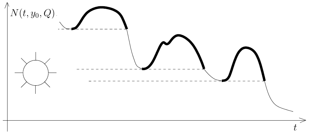
Fig. 1: Falling sum theorem

The following result mainly concerns with the continuity of the minimal norm function.

Theorem 9.

Given $y_{0}\in L^{2}(\Omega)$ and $Q\in\mathcal{F}$, the minimal norm function $t\rightarrow N(t,y_{0},Q)$ is locally Lipschitz continuous over $\mathbb{R}^{+}$. If further assume that $y_{0}$ and $Q$ satisfy (11), then $\lim_{t\rightarrow 0^{+}}N(t,y_{0},Q)=+\infty$.

Proof.

We divide the proof into following three steps:

Step 1. To show that for each $y_{0}\in L^{2}(\Omega)$, $Q\in\mathcal{F}$ and each $\delta>0$, there is $C_{1}(\Omega,\omega,Q,\delta)>0$ so that

$$N(T,y_{0},Q)\leq C_{1}(\Omega,\omega,Q,\delta)(\|y_{0}\|+1)\;\;\mbox{for all}\;\;T>\delta$$ (30)

     Arbitrarily fix $y_{0}\in L^{2}(\Omega)$, $Q\in\mathcal{F}$ and $\delta>0$. Since the heat equation holds the approximate controllability (see [8, Theorem 1.4]) and the $L^{\infty}$-null controllability (see, for instance, [8, Proposition 3.2]), there is $v_{\delta}$ (only depending on $\delta$, $Q$, $\Omega$ and $\omega$) and $v_{\delta}^{\prime}$ so that

$$\hat{y}(\delta;0,v_{\delta})\in Q,\;\;\hat{y}(\delta;y_{0},v_{\delta}^{\prime})=0\;\;\mbox{and}\;\;\|v_{\delta}^{\prime}\|_{L^{\infty}(0,\delta;L^{2}(\Omega))}\leq C(\Omega,\omega,\delta)\|y_{0}\|.$$ (31)

Still write $v_{\delta}^{\prime}$ for its zero extension over $\mathbb{R}^{+}$. Arbitrarily fix $T>\delta$. Define a control $\widehat{v}_{T}$ over $(0,T)$ as follow:

$$\widehat{v}_{T}(t)\triangleq\left\{\begin{array}[]{ll}v_{\delta}^{\prime}(t),~{}t\in(0,T-\delta],\\ v_{\delta}^{\prime}(t)+v_{\delta}(t-T+\delta),~{}t\in(T-\delta,T).\end{array}\right.$$ (34)

From (34) and the last conclusion in (31), we find that

$$\|\widehat{v}_{T}\|_{L^{\infty}(0,T;L^{2}(\Omega))}\leq C(\Omega,\omega,\delta)\|y_{0}\|+\|v_{\delta}\|_{L^{\infty}(0,\delta;L^{2}(\Omega))}.$$ (35)

Meanwhile, from (34) and the first two conclusions in (31), we see that

$$\hat{y}(T;y_{0},\widehat{v}_{T}) = e^{\Delta T}y_{0}+\int_{0}^{\delta}e^{\Delta(T-t)}\chi_{\omega}v_{\delta}^{\prime}(t)\mathrm{d}t+\int_{T-\delta}^{T}e^{\Delta(T-t)}\chi_{\omega}v_{\delta}(t-T+\delta)\mathrm{d}t$$

$$= e^{\Delta(T-\delta)}\hat{y}(\delta;y_{0},v_{\delta}^{\prime})+\int_{0}^{\delta}e^{\Delta(\delta-t)}\chi_{\omega}v_{\delta}(t)\mathrm{d}t=\hat{y}(\delta;0,v_{\delta})\in Q,$$

which shows that $\widehat{v}_{T}$ is an admissible control to $(NP)^{T,y_{0}}_{Q}$. This, along with the optimality of $N(T,y_{0},Q)$ and (35), indicates that

$$N(T,y_{0},Q)\leq\|\widehat{v}_{T}\|_{L^{\infty}(0,T;L^{2}(\Omega))}\leq C(\Omega,\omega,\delta)\|y_{0}\|+\|v_{\delta}\|_{L^{\infty}(0,\delta;L^{2}(\Omega))},$$

which leads to (30). Here we used the fact that $v_{\delta}$ only depends on $\delta$, $Q$, $\Omega$ and $\omega$.

Step 2. To show that for each $y_{0}\in L^{2}(\Omega)$, $Q\in\mathcal{F}$ and each triplet $(\delta,T_{1},T_{2})$, with $0<\delta<T_{2}/2<T_{1}<T_{2}$, there exists a constant $C_{2}(\Omega,\omega,Q,\delta)>0$ so that

$$|N(T_{1},y_{0},Q)-N(T_{2},y_{0},Q)|\leq C_{2}(\Omega,\omega,Q,\delta)(\|y_{0}\|+1)|T_{1}-T_{2}|$$ (36)

     Arbitrarily fix $y_{0}\in L^{2}(\Omega)$, $Q\in\mathcal{F}$ and $(\delta,T_{1},T_{2})$ as required. To prove (36), it suffices to show that for some $C_{2}(\Omega,\omega,Q,\delta)>0$,

$$N(T_{1},y_{0},Q)-N(T_{2},y_{0},Q)\leq C_{2}(\Omega,\omega,Q,\delta)(\|y_{0}\|+1)(T_{2}-T_{1});$$ (37)

$$N(T_{2},y_{0},Q)-N(T_{1},y_{0},Q)\leq C_{2}(\Omega,\omega,Q,\delta)(\|y_{0}\|+1)(T_{2}-T_{1}).$$ (38)

To show (37), we first note that $(NP)^{T_{2},y_{0}}_{Q}$ has a minimal norm control $v_{T_{2}}^{*}$ (see Theorem 4). Thus,

$$\hat{y}(T_{2};y_{0},v_{T_{2}}^{*})\in Q\;\;\mbox{and}\;\;\|v_{T_{2}}^{*}\|_{L^{\infty}(0,T_{2};L^{2}(\Omega))}=N(T_{2},y_{0},Q).$$ (39)

We set

$$z_{T_{1}}\triangleq\hat{y}(3T_{2}/4;0,\chi_{(0,T_{2}-T_{1})}v_{T_{2}}^{*}).$$ (40)

Since $T_{2}/4>\delta/4$, it follows from the $L^{\infty}$-null controllability for the heat equation (see [8, Proposition 3.2]) that there is $f_{1}\in L^{\infty}(0,T_{2}/4;L^{2}(\Omega))$, with $f_{1}=0$ over $(\delta/4,T_{2}/4)$, so that

$$0=\hat{y}(\delta/4;z_{T_{1}},f_{1})=\hat{y}(T_{2}/4;z_{T_{1}},f_{1});$$ (41)

$$\|f_{1}\|_{L^{\infty}(0,T_{2}/4;L^{2}(\Omega))}\leq C(\Omega,\omega,\delta/4)\|z_{T_{1}}\|.$$ (42)

Since $T_{2}-T_{1}<3T_{2}/4$, from (40) and (41), we can easily check that

$$\hat{y}(T_{2};0,\chi_{(0,T_{2}-T_{1})}v_{T_{2}}^{*}) = e^{\Delta T_{2}/4}z_{T_{1}}=-\int_{0}^{T_{2}/4}e^{\Delta(T_{2}/4-t)}\chi_{\omega}f_{1}(t)\mathrm{d}t.$$ (43)

We next set

$$w_{T_{1}}\triangleq e^{\Delta(T_{1}-T_{2}/4)}(e^{\Delta(T_{2}-T_{1})}y_{0}-y_{0}).$$ (44)

Since $T_{2}/4>\delta/4$, by [8, Proposition 3.2], we find that there is $f_{2}\in L^{\infty}(0,T_{2}/4;L^{2}(\Omega))$, with $f_{2}=0$ over $(\delta/4,T_{2}/4)$, so that

$$0=\hat{y}(\delta/4;w_{T_{1}},f_{2})=\hat{y}(T_{2}/4;w_{T_{1}},f_{2});$$ (45)

$$\|f_{2}\|_{L^{\infty}(0,T_{2}/4;L^{2}(\Omega))}\leq C(\Omega,\omega,\delta/4)\|w_{T_{1}}\|.$$ (46)

From (44) and (45), we see that

$$e^{\Delta T_{2}}y_{0}-e^{\Delta T_{1}}y_{0} = e^{\Delta T_{2}/4}w_{T_{1}}=-\int_{0}^{T_{2}/4}e^{\Delta(T_{2}/4-t)}\chi_{\omega}f_{2}(t)\mathrm{d}t.$$ (47)

Now we define a control $f_{3}$ over $(0,T_{1})$ by

$$f_{3}(t)\triangleq\left\{\begin{array}[]{ll}v_{T_{2}}^{*}(t-T_{1}+T_{2}),&t\in(0,T_{1}-T_{2}/4),\\ v_{T_{2}}^{*}(t-T_{1}+T_{2})-f_{1}(t-T_{1}+T_{2}/4)&\\ -f_{2}(t-T_{1}+T_{2}/4),&t\in(T_{1}-T_{2}/4,T_{1}).\end{array}\right.$$ (51)

Two observations are given in order: First, by (51), (42) and (46), we see that

$$\|f_{3}\|_{L^{\infty}(0,T_{1};L^{2}(\Omega))}\leq\|v_{T_{2}}^{*}\|_{L^{\infty}(T_{2}-T_{1},T_{2};L^{2}(\Omega))}+C(\Omega,\omega,\delta/4)\big{(}\|z_{T_{1}}\|+\|w_{T_{1}}\|\big{)}.$$

Second, by (51), (43), (47) and (40), after some computations, one can easily check that $\hat{y}(T_{1};y_{0},f_{3})=\hat{y}(T_{2};y_{0},v^{*}_{T_{2}})$, which, along with the first conclusion in (39), yields that $f_{3}$ is an admissible control to $(NP)^{T_{1},y_{0}}_{Q}$. These two observations, together with the optimality of $N(T_{1},y_{0},Q)$, indicate that

$$N(T_{1},y_{0},Q)\leq\|v_{T_{2}}^{*}\|_{L^{\infty}(0,T_{2};L^{2}(\Omega))}+C(\Omega,\omega,\delta/4)\big{(}\|z_{T_{1}}\|+\|w_{T_{1}}\|\big{)}.$$

This, along with the second conclusion in (39), (40) and (44), implies that

$$N(T_{1},y_{0},Q) \leq N(T_{2},y_{0},Q)+C(\Omega,\omega,\delta/4)\,\big{[}(T_{2}-T_{1})N(T_{2},y_{0},Q)$$ (52)

$$+\|e^{\Delta(T_{1}-T_{2}/4)}(e^{\Delta(T_{2}-T_{1})}y_{0}-y_{0})\|\big{]}.$$

Meanwhile, since $T_{1}-T_{2}/4>T_{2}/4>\delta/2$, it follows that

$$\|e^{\Delta(T_{1}-T_{2}/4)}(e^{\Delta(T_{2}-T_{1})}y_{0}-y_{0})\|$$ (53)

$$\leq \|e^{\Delta T_{2}/4}(e^{\Delta(T_{2}-T_{1})}y_{0}-y_{0})\|=\big{\|}\int_{0}^{T_{2}-T_{1}}\Delta e^{\Delta s}(e^{\Delta T_{2}/4}y_{0})\mathrm{d}s\big{\|}$$

$$\leq (T_{2}-T_{1})\|\Delta e^{\Delta T_{2}/4}y_{0}\|\leq 4(T_{2}-T_{1})\|y_{0}\|/T_{2}\leq 2(T_{2}-T_{1})\|y_{0}\|/\delta.~{}~{}~{}~{}~{}$$

From (52), (53) and (30), we obtain (37).

To show (38), we note that $(NP)^{T_{1},y_{0}}_{Q}$ has a minimal norm control $v_{T_{1}}^{*}$ (see Theorem 4). Thus,

$$\hat{y}(T_{1};y_{0},v_{T_{1}}^{*})\in Q\;\;\mbox{and}\;\;\|v_{T_{1}}^{*}\|_{L^{\infty}(0,T_{1};L^{2}(\Omega))}=N(T_{1},y_{0},Q).$$ (54)

We define a control $f_{4}$ by

$$f_{4}(t)\triangleq\left\{\begin{array}[]{ll}0,&t\in(0,T_{2}-T_{1}),\\ v_{T_{1}}^{*}(t-T_{2}+T_{1}),&t\in(T_{2}-T_{1},3T_{2}/4),\\ v_{T_{1}}^{*}(t-T_{2}+T_{1})+f_{2}(t-3T_{2}/4),&t\in(3T_{2}/4,T_{2}),\end{array}\right.$$ (58)

where $f_{2}$ is given by (45). By (58) and (47), after some direct computations, we find that $\hat{y}(T_{2};y_{0},f_{4})=\hat{y}(T_{1};y_{0},v^{*}_{T_{1}})$, which, along with the first conclusion in (54), shows that $f_{4}$ is an admissible control to $(NP)^{T_{2},y_{0}}_{Q}$. This, together with the optimality of $N(T_{2},y_{0},Q)$ and (58), yields that

$$N(T_{2},y_{0},Q)\leq\|f_{4}\|_{L^{\infty}(0,T_{2};L^{2}(\Omega))}\leq\|v^{*}_{T_{1}}\|_{L^{\infty}(0,T_{1};L^{2}(\Omega))}+\|f_{2}\|_{L^{\infty}(0,T_{2}/4;L^{2}(\Omega))}.$$

Then we see from the second conclusion in (54) and (46) that

$$N(T_{2},y_{0},Q)\leq N(T_{1},y_{0},Q)+C(\Omega,\omega,\delta/4)\|w_{T_{1}}\|.$$

This, along with (44) and (53), leads to (38).

Step 3. To show that $\lim_{t\rightarrow 0^{+}}N(t,y_{0},Q)=+\infty$, when $(y_{0},Q)\in L^{2}(\Omega)\times\mathcal{F}$ verifies (11)

By contradiction, we suppose that it were not true. Then there would be $(y_{0},Q)\in L^{2}(\Omega)\times\mathcal{F}$, with (11); and $\{t_{n}\}\subset\mathbb{R}^{+}$, with $\lim_{n\rightarrow+\infty}t_{n}=0$, so that

$$\sup_{n\in\mathbb{N}^{+}}N(t_{n},y_{0},Q)\leq C\;\;\mbox{for some}\;\;C>0.$$ (59)

By Theorem 4, we find that for each $n\in\mathbb{N}^{+}$, $(NP)^{t_{n},y_{0}}_{Q}$ has a minimal norm control $v_{n}$ satisfying that

$$\hat{y}(t_{n};y_{0},v_{n})\in Q\;\;\mbox{ and }\;\;\|v_{n}\|_{L^{\infty}(0,T_{n};L^{2}(\Omega))}=N(t_{n},y_{0},Q).$$ (60)

Extend $v_{n}$ over $\mathbb{R}^{+}$ by setting it to be zero over $[t_{n},+\infty)$ and still denote the extension in the same manner. Since $\lim_{n\rightarrow+\infty}t_{n}=0$, it follows from the second conclusion in (60) and (59) that $\chi_{(0,t_{n})}v_{n}\rightarrow 0$ strongly in $L^{2}(\mathbb{R}^{+};L^{2}(\Omega))$, as $n\rightarrow+\infty$. This, together with the first conclusion in (60) and the fact that $\lim_{n\rightarrow+\infty}t_{n}=0$, yields that $y_{0}=\lim_{n\rightarrow+\infty}\hat{y}(t_{n};y_{0},v_{n})\in Q$, which contradicts (11). Hence, the conclusion in Step 3 is true.

In summary, we end the proof of this theorem. ∎

By Theorem 9 and Theorem 7, we can prove the following Proposition 10, which will be used in the proof of Theorem 3.

Proposition 10.

Let $y_{0}\in L^{2}(\Omega)$ and $Q\in\mathcal{F}$ satisfy (11). Then the following two conclusions are valid:
(i) For each $M\in[0,+\infty)$, it holds that $T(M,y_{0},Q)\in(0,+\infty]$.
(ii) For each $M\in[0,+\infty)$, with $T(M,y_{0},Q)<+\infty$, it stands that

$$N(T(M,y_{0},Q),y_{0},Q)=M.$$ (61)

Proof.

Arbitrarily fix $y_{0}$ and $Q$ satisfying (11). We will prove (i)-(ii) one by one.

(i) By contradiction, we suppose that the conclusion (i) were not true. Then there would be $M\in[0,+\infty)$ so that $T(M,y_{0},Q)=0$. This, along with (9), yields that there exists $\{\hat{t}_{n}\}\subset[0,+\infty)$ and $\{u_{n}\}\subset\mathcal{U}^{M}$ so that

$$\lim_{n\rightarrow+\infty}\hat{t}_{n}=0,\;\;y(\hat{t}_{n};y_{0},u_{n})\in Q\;\;\mbox{and}\;\;\|u_{n}\|_{L^{\infty}(\mathbb{R}^{+};L^{2}(\Omega))}\leq M.$$ (62)

By the last inequality in (62), $\chi_{(0,\hat{t}_{n})}u_{n}\rightarrow 0$ strongly in $L^{2}(\mathbb{R}^{+};L^{2}(\Omega))$. This, along with the first two conclusions in (62), yields that $y_{0}=\lim_{n\rightarrow+\infty}y(\hat{t}_{n};y_{0},u_{n})\in Q$, which contradicts (11). So the conclusion (i) is true.

(ii) Arbitrarily fix $M\in[0,+\infty)$ so that $T(M,y_{0},Q)<+\infty$. By the conclusion (i) in this proposition, we find that $0<T(M,y_{0},Q)<+\infty$. This, along with (22) (see Theorem 7) and (21), indicates that $\mathcal{J}_{M}\neq\emptyset$. Thus, by (22), (21) and (20), there is a sequence $\{t_{n}\}\subset\mathbb{R}^{+}$ so that

$$\lim_{n\rightarrow+\infty}t_{n}=T(M,y_{0},Q)\;\;\mbox{and}\;\;N(t_{n},y_{0},Q)\leq M\;\;\mbox{for all}\;\;n\in\mathbb{N}^{+}.$$

Since $T(M,y_{0},Q)\in(0,+\infty)$, the above conclusions, together with the continuity of the minimal norm function at $T(M,y_{0},Q)\in(0,+\infty)$ (see Theorem 9), yield that

$$N(T(M,y_{0},Q),y_{0},Q)\leq M.$$ (63)

We next prove (61). By contradiction, we suppose that it were not true. Then by (63), we would have that $N(T(M,y_{0},Q),y_{0},Q)<M$. This, along with the continuity of the minimal norm function at $T(M,y_{0},Q)$, yields that there is $\delta_{0}\in\big{(}0,T(M,y_{0},Q)\big{)}$ so that $N(T(M,y_{0},Q)-\delta_{0},y_{0},Q)<M$. Then it follows from (20) that $T(M,y_{0},Q)-\delta_{0}\in\mathcal{J}_{M}$, which contradicts (22). Hence (61) is true.

In summary, we end the proof of this proposition. ∎

2.3 Proof of Theorem 3

Let $y_{0}\in L^{2}(\Omega)$ and $Q\in\mathcal{F}$ satisfying (11). We prove the conclusions (i)-(iii) one by one.

(i) Arbitrarily fix $(M,T)$ so that

$$(M,T)\in(\mathcal{G}T)_{y_{0},Q}\setminus(\mathcal{K}N)_{y_{0},Q}.$$ (64)

Then it follows from (12) that

$$0<T=T(M,y_{0},Q)<+\infty.$$ (65)

CLAIM ONE: The problems $(NP)^{T,y_{0}}_{Q}$ and $(TP)^{M,y_{0}}_{Q}$ have minimal norm and minimal time controls, respectively. Indeed, since $0<T<+\infty$ (see (65)), it follows from Theorem 4 that $(NP)^{T,y_{0}}_{Q}$ has at least one minimal norm control. Meanwhile, since $T(M,y_{0},Q)<+\infty$ (see (65)), it follows from (ii) of Definition 1 that $(TP)^{M,y_{0}}_{Q}$ has at least one admissible control. Then by a standard way (see, for instance, the proof of [7, Lemma 1.1]), we can prove that $(TP)^{M,y_{0}}_{Q}$ has at least one minimal time control.

CLAIM TWO: For an arbitrarily fixed minimal time control $u^{*}_{1}$ to $(TP)^{M,y_{0}}_{Q}$, $u^{*}_{1}|_{(0,T)}$ is a minimal norm control to $(NP)^{T,y_{0}}_{Q}$. Indeed, by the optimality of $u^{*}_{1}$ and (65), we have that

$$y(T;y_{0},u_{1}^{*})=y(T(M,y_{0},Q);y_{0},u_{1}^{*})\in Q\;\;\mbox{and}\;\;\|u_{1}^{*}\|_{L^{\infty}(\mathbb{R}^{+};L^{2}(\Omega))}\leq M.$$ (66)

By the first conclusion in (66), we see that $u_{1}^{*}|_{(0,T)}$ is an admissible control to $(NP)^{T,y_{0}}_{Q}$. This, along with the optimality of $N(T,y_{0},Q)$ and the second conclusion in (66), yields that

$$N(T,y_{0},Q)\leq\|u_{1}^{*}|_{(0,T)}\|_{L^{\infty}(0,T;L^{2}(\Omega))}\leq M.$$ (67)

Meanwhile, by (65), we can apply (ii) of Proposition 10 to find that

$$N(T,y_{0},Q)=N(T(M,y_{0},Q),y_{0},Q)=M.$$ (68)

From (67) and (68), we see that

$$\|u_{1}^{*}|_{(0,T)}\|_{L^{\infty}(0,T;L^{2}(\Omega))}=N(T,y_{0},Q).$$

Since $u_{1}^{*}|_{(0,T)}$ is an admissible control to $(NP)^{T,y_{0}}_{Q}$, the above shows that $u_{1}^{*}|_{(0,T)}$ is a minimal norm control to $(NP)^{T,y_{0}}_{Q}$.

CLAIM THREE: For an arbitrarily fixed minimal norm control $v_{1}^{*}$ to $(NP)^{T,y_{0}}_{Q}$, the zero extension of $v_{1}^{*}$ over $\mathbb{R}^{+}$, denoted by $\widetilde{v}_{1}^{*}$, is a minimal time control to $(TP)^{M,y_{0}}_{Q}$. Indeed, by the optimality of $v_{1}^{*}$, one can easily check that

$$y(T;y_{0},\widetilde{v}_{1}^{*})\in Q\;\;\mbox{and}\;\;\|\widetilde{v}_{1}^{*}\|_{L^{\infty}(\mathbb{R}^{+};L^{2}(\Omega))}=N(T,y_{0},Q).$$

From this, (65), (68) and (i) of Definition 1, we find that $\widetilde{v}_{1}^{*}$ is a minimal time control to $(TP)^{M,y_{0}}_{Q}$.

Now, by the above three claims and Definition 2, we see that the problems $(TP)^{M,y_{0}}_{Q}$ and $(NP)^{T,y_{0}}_{Q}$ are equivalent.

Finally, we claim that

$$N(T,y_{0},Q)\neq 0.$$ (69)

When (69) is proved, we can easily check that the null control (defined on $(0,T)$) is not a minimal norm control to $(NP)^{T,y_{0}}_{Q}$. Then by the equivalence of $(TP)^{M,y_{0}}_{Q}$ and $(NP)^{T,y_{0}}_{Q}$, we can easily prove that the null control (defined on $\mathbb{R}^{+}$) is not a minimal time control to $(TP)^{M,y_{0}}_{Q}$.

The remainder is to show (69). By contradiction, suppose that (69) were not true. Then we would have that $N(T,y_{0},Q)=0$. This, together with (68), yields that $M=0$. From this and (13), we get that $(M,T)\in(\mathcal{K}N)_{y_{0},Q}$, which contradicts (64). Therefore, (69) is true. This ends the proof of the conclusion (i) in Theorem 3.

(ii) Without loss of generality, we can assume that $(\mathcal{K}N)_{y_{0},Q}\neq\emptyset$. Arbitrarily fix

$$(M,T)\in(\mathcal{K}N)_{y_{0},Q}.$$ (70)

By Definition 2, we see that in order to prove the conclusion (ii), it suffices to show that the null controls (defined on $(0,T)$ and $\mathbb{R}^{+}$, respectively) are the unique minimal norm control and the unique minimal time control to $(NP)^{T,y_{0}}_{Q}$ and $(TP)^{M,y_{0}}_{Q}$, respectively. To this end, we observe from (70) and (13) that

$$0<T<+\infty,\;M=0\;\;\mbox{and}\;\;N(T,y_{0},Q)=0.$$ (71)

By the first conclusion of (71) and Theorem 4, we see that $(NP)^{T,y_{0}}_{Q}$ has at least one minimal norm control. This, along with the last conclusion in (71), implies that the null control (defined on $(0,T)$) is the unique minimal norm control to $(NP)^{T,y_{0}}_{Q}$. From this, it follows that $\hat{y}(T;y_{0},0)\in Q$, from which, one can easily check that the null control (defined on $\mathbb{R}^{+}$) is admissible for $(TP)^{M,y_{0}}_{Q}$. Then by a standard way (see, for instance, the proof of [7, Lemma 1.1]), we can prove that $(TP)^{M,y_{0}}_{Q}$ has at least one minimal time control. This, along with the second conclusion in (71), indicates that the null control is the unique minimal time control to $(TP)^{M,y_{0}}_{Q}$. This ends the proof of the conclusion (ii) in Theorem 3.

(iii) By contradiction, suppose that the conclusion (iii) were not true. Then there would be a pair

$$(M,T)\in[0,+\infty)\times(0,+\infty)\setminus\big{(}(\mathcal{G}T)_{y_{0},Q}\cup(\mathcal{K}N)_{y_{0},Q}\big{)}$$ (72)

so that $(TP)^{M,y_{0}}_{Q}$ and $(NP)^{T,y_{0}}_{Q}$ are equivalent. The key to get a contradiction is to prove that

$$T(M,y_{0},Q)=T.$$ (73)

When this is proved, we see from (73) and (12) that $(M,T)\in(\mathcal{G}T)_{y_{0},Q}$. (Notice that $0<T<+\infty$ and $0\leq M<+\infty$.) This contradicts (72). Hence, the conclusion (iii) is true.

We now prove (73). Since $(TP)^{M,y_{0}}_{Q}$ and $(NP)^{T,y_{0}}_{Q}$ are equivalent, two facts are derived from Definition 2: First, $(NP)^{T,y_{0}}_{Q}$ has a minimal norm control $v_{2}^{*}$; Second, the zero extension of $v_{2}^{*}$ over $\mathbb{R}^{+}$, denoted by $\widetilde{v}_{2}^{*}$, is a minimal time control to $(TP)^{M,y_{0}}_{Q}$. From these two facts, we can easily check that $T(M,y_{0},Q)\leq T$. This, along with (i) of Proposition 10, shows that

$$0<T(M,y_{0},Q)\leq T.$$ (74)

By contradiction, we suppose that (73) were not true. Then by (74) and (72), we would have that

$$0<T(M,y_{0},Q)<T<+\infty.$$ (75)

It follows from (75) and (ii) of Definition 1 that $(TP)^{M,y_{0}}_{Q}$ has at least one admissible control. Then by a standard way (see, for instance, the proof of [7, Lemma 1.1]), we can prove that $(TP)^{M,y_{0}}_{Q}$ has a minimal time control $u^{*}$. Thus we have that

$$y(T(M,y_{0},Q);y_{0},u^{*})\in Q\;\;\mbox{and}\;\;\|u^{*}\|_{L^{\infty}(\mathbb{R}^{+};L^{2}(\Omega))}\leq M.$$ (76)

Arbitrarily take $\hat{z}\in L^{2}(\Omega)\setminus\{0\}$. Define

$$\hat{u}_{0}^{*}(t)=\left\{\begin{array}[]{l}u^{*}(t),~{}t\in\big{(}0,T(M,y_{0},Q)\big{)},\\ 0,~{}t\in[T(M,y_{0},Q),+\infty);\end{array}\right.\;\;\hat{u}_{M}^{*}(t)=\left\{\begin{array}[]{l}u^{*}(t),~{}t\in\big{(}0,T(M,y_{0},Q)\big{)},\\ M\frac{\hat{z}}{\|\hat{z}\|},~{}t\in[T(M,y_{0},Q),+\infty).\end{array}\right.$$

From these and (76), we see that $\hat{u}_{0}^{*}$ and $\hat{u}_{M}^{*}$ are minimal time controls to $(TP)^{M,y_{0}}_{Q}$. By the equivalence of $(TP)^{M,y_{0}}_{Q}$ and $(NP)^{T,y_{0}}_{Q}$, we find that $\hat{u}_{0}^{*}|_{(0,T)}$ and $\hat{u}_{M}^{*}|_{(0,T)}$ are minimal norm controls to $(NP)^{T,y_{0}}_{Q}$. This, along with (75) and Theorem 5, indicates that for a.e. $t\in\big{(}T(M,y_{0},Q),T\big{)}$,

$$N(T,y_{0},Q)=\|\hat{u}_{0}^{*}(t)\|=0\;\;\mbox{and}\;\;N(T,y_{0},Q)=\|\hat{u}_{M}^{*}(t)\|=M.$$

From these, it follows that $N(T,y_{0},Q)=M=0$. This, along with (13), yields that $(M,T)\in(\mathcal{K}N)_{y_{0},Q}$, which contradicts (72). Thus, (73) is true. This ends the proof of the conclusion (iii) in Theorem 3.

In summary, we conclude that the conclusions (i), (ii) and (iii) are true. This completes the proof of Theorem 3.

3 Further illustrations

The aim of this section is to construct an example where the minimal norm function $T\rightarrow N(T,y_{0},Q)$ is not decreasing, the set $(\mathcal{K}N)_{y_{0},Q}$ is not empty and the set $(\mathcal{G}T)_{y_{0},Q}$ is not connected. This example may help us to understand Theorem 3 better.

Theorem 11.

There exists $Q\in\mathcal{F}$ and $y_{0}\in L^{2}(\Omega)\setminus Q$ so that the following propositions are true:
(i) The function $T\rightarrow N(T,y_{0},Q)$ is not decreasing;
(ii) The set $(\mathcal{K}N)_{y_{0},Q}\neq\emptyset$ and the set $(\mathcal{G}T)_{y_{0},Q}$ is not connected.

To prove the above theorem, we need some preliminaries. The following lemma concerns with some kind of continuity of the map $Q\rightarrow N(T,y_{0},Q)$.

Lemma 12.

Let $E\subset L^{2}(\Omega)$ be a finite dimension subspace, with its orthogonal space $E^{\perp}$. Suppose that $\{S_{n}\}_{n=1}^{+\infty}\subset E$ is an increasing sequence of bounded closed convex subsets. Assume that $S\triangleq\cup_{n=1}^{+\infty}S_{n}$ verifies that

$$\hat{Q}\triangleq\bar{S}\oplus B_{E^{\perp}}\in\mathcal{F},$$ (78)

where $\bar{S}$ and $B_{E^{\perp}}$ denote the closure of $S$ in $E$ and the closed unit ball in $E^{\perp}$, respectively. Let

$$Q_{n}\triangleq S_{n}\oplus B_{E^{\perp}}\;\;\mbox{for each}\;\;n\in\mathbb{N}^{+}.$$ (79)

Then for all $n$ large enough, $Q_{n}\in\mathcal{F}$; and for all $y_{0}\in L^{2}(\Omega)$ and for all $a$ and $b$, with $0<a<b<+\infty$,

$$N(T,y_{0},Q_{n})\rightarrow N(T,y_{0},\hat{Q})\mbox{ uniformly w.r.t. }T\in[a,b],\;\;\mbox{as}\;\;n\rightarrow\infty.$$ (80)

Proof.

By using [21, Theorem 1.1.14] and (78) and the definition of $\mathcal{F}$, we see that $\bar{S}$ has a nonempty interior in $E$. Then, by the finite dimensionality and the convexity of $S$, one can easily check that $S$ has a nonempty interior in $E$. Since $S=\cup_{n=1}^{\infty}S_{n}\subset E$, it follows from the Baire Category Theorem that $S_{N_{0}}$ has a nonempty interior in $E$ for some $N_{0}\in\mathbb{N}^{+}$. Thus, by the monotonicity of $\{S_{n}\}_{n=1}^{\infty}$ and the definition of $Q_{n}$, there exists a closed ball $B_{r}(y_{d})$ in $L^{2}(\Omega)$, centered at $y_{d}\in L^{2}(\Omega)$ and of radius $r>0$, so that

$$B_{r}(y_{d})\subset Q_{N_{0}}\subset Q_{n}\;\;\mbox{for all}\;\;n\geq N_{0}.$$ (81)

From (79) and (81), we see that when $n\geq N_{0}$, $Q_{n}\in\mathcal{F}$.

Now we arbitrarily fix $y_{0}\in L^{2}(\Omega)$ and $0<a<b<+\infty$. Then arbitrarily fix $T\in[a,b]$. The rest proof is divided into the following four steps.

Step 1. To show that there exists $C\triangleq C(\Omega,b,y_{d},r)>0$ (independent of $T\in[a,b]$), $\hat{y}_{0,T}\in L^{2}(\Omega)$ and $\hat{y}_{d}\in L^{2}(\Omega)$ (independent of $T\in[a,b]$) so that

$$\|\hat{y}_{d}-y_{d}\|\leq r/2,~{}\hat{y}_{d}=e^{\Delta T}\hat{y}_{0,T}\;\;\mbox{and}\;\;\|\hat{y}_{0,T}\|\leq C$$ (82)

     Let $\{\lambda_{j}\}_{j=1}^{+\infty}$ be the family of all eigenvalues of $-\Delta$ with the zero Dirichlet boundary condition so that

$$0<\lambda_{1}\leq\lambda_{2}\leq\cdots\;\;\mbox{and}\;\;\lim_{j\rightarrow+\infty}\lambda_{j}=\infty.$$ (83)

Write $\{e_{j}\}_{j=1}^{+\infty}$ for the family of the corresponding normalized eigenvectors. Since $y_{d}\in L^{2}(\Omega)$, we can choose a positive integer $K\triangleq K(y_{d},r)$ large enough so that $\Sigma_{j=K+1}^{\infty}\langle y_{d},e_{j}\rangle^{2}\leq r^{2}/4$. Let $\hat{y}_{d}\triangleq\Sigma^{K}_{j=1}\langle y_{d},e_{j}\rangle e_{j}$ and $\hat{y}_{0,T}\triangleq\Sigma^{K}_{j=1}e^{\lambda_{j}T}\langle y_{d},e_{j}\rangle e_{j}$. Then, one can easily check that $\hat{y}_{d}$ and $y_{0,T}$ verify (82) for some $C\triangleq C(\Omega,b,y_{d},r)>0$.

Step 2. To prove that for each $n\geq N_{0}$,

$$N(T,y_{0},\hat{Q})\leq N(T,y_{0},Q_{n})$$ (84)

     Since $Q_{n}\in\mathcal{F}$ for each $n\geq N_{0}$, we find from Theorem 4 that for each $n\geq N_{0}$, $(NP)^{T,y_{0}}_{Q_{n}}$ has at least one minimal norm control. Since $S_{n}\subset\bar{S}$ for each $n$, we have that $Q_{n}\subset\hat{Q}$ for all $n\in\mathbb{N}^{+}$. Thus, when $n\geq N_{0}$, each minimal norm control to $(NP)^{T,y_{0}}_{Q_{n}}$ is an admissible control to $(NP)^{T,y_{0}}_{\hat{Q}}$. This, along with the optimality of $N(T,y_{0},\hat{Q})$, leads to (84).

Step 3. To prove that for each $\lambda\in(0,1)$, there is $N_{\lambda}\geq N_{0}$ (independent of $T\in[a,b]$) so that when $n\geq N_{\lambda}$,

$$N(T,y_{0},Q_{n})-N(T,y_{0},\hat{Q})\leq C(\Omega,\omega,a)(1-\lambda)\|y_{0}-\hat{y}_{0,T}\|$$ (85)

for some $C(\Omega,\omega,a)>0$ independent of $T\in[a,b]$ and $\lambda\in(0,1)$, where $\hat{y}_{0,T}$ is given by Step 1

Let $u^{*}$ be a minimal norm control to $(NP)^{T,y_{0}}_{\hat{Q}}$. (Its existence is ensured by (78) and Theorem 4.) Then

$$\hat{y}(T;y_{0},u^{*})\in\hat{Q}\;\;\mbox{and}\;\;\|u^{*}\|_{L^{\infty}(0,T;L^{2}(\Omega))}=N(T,y_{0},\hat{Q}).$$ (86)

Let $\hat{y}_{d}$ be given by Step 1. Arbitrarily fix $\lambda\in(0,1)$. At the end of the proof of this lemma, we will prove the following conclusion: There is $N_{\lambda}\geq N_{0}$ so that

$$\lambda(\hat{Q}-\{\hat{y}_{d}\})\subset Q_{n}-\{\hat{y}_{d}\},\;\;\mbox{when}\;\;n\geq N_{\lambda}.$$ (87)

We now suppose that (87) is true. Then, arbitrarily fix $n\geq N_{\lambda}$. From the second conclusion in (82), the first conclusion in (86) and (87), we find that

$$\hat{y}(T;\lambda(y_{0}-\hat{y}_{0,T}),\lambda u^{*})=\lambda(\hat{y}(T;y_{0},u^{*})-\hat{y}_{d})\in Q_{n}-\{\hat{y}_{d}\}.$$ (88)

Meanwhile, since $a\leq T\leq b$, by the $L^{\infty}$-null controllability for the heat equation (see [8, Proposition 3.2]), there is $v_{n}\in{L^{\infty}(0,T;L^{2}(\Omega)})$, with supp $v_{n}\subset(0,a)$, so that

$$\hat{y}(T;(1-\lambda)(y_{0}-\hat{y}_{0,T}),v_{n})=0$$ (89)

and so that

$$~{}~{}~{}~{}~{}\|v_{n}\|_{L^{\infty}(0,T;L^{2}(\Omega))}\leq C(\Omega,\omega,a)(1-\lambda)\|y_{0}-\hat{y}_{0,T}\|\;\;\mbox{for some}\;C(\Omega,\omega,a)>0.$$ (90)

Now, it follows from the second conclusion in (82), (89) and (88) that

$$\hat{y}(T;y_{0},\lambda u^{*}+v_{n}) = e^{\Delta T}\hat{y}_{0,T}+\hat{y}(T;y_{0}-\hat{y}_{0,T},\lambda u^{*}+v_{n})$$

$$= \hat{y}_{d}+\hat{y}(T;\lambda(y_{0}-\hat{y}_{0,T}),\lambda u^{*})\in Q_{n}.$$

Thus, $\lambda u^{*}+v_{n}$ is an admissible control to $(NP)^{T,y_{0}}_{Q_{n}}$, which, along with the optimality of $N(T,y_{0},Q_{n})$, yields that

$$N(T,y_{0},Q_{n})\leq\|\lambda u^{*}+v_{n}\|_{L^{\infty}(0,T;L^{2}(\Omega))}.$$

This, together with the second conclusion in (86) and (90), yields that

$$N(T,y_{0},Q_{n})\leq\lambda N(T,y_{0},\hat{Q})+C(\Omega,\omega,a)(1-\lambda)\|y_{0}-\hat{y}_{0,T}\|.$$

Since $\lambda\in(0,1)$, the above inequality leads to (85). This ends the proof of Step 3.

Step 4. To verify (80)

Given $\varepsilon\in(0,1)$, it follows by (85) and (84) that when $n\geq N_{1-\varepsilon}$ (where $N_{1-\varepsilon}$ is given by Step 3, with $\lambda=1-\varepsilon$),

$$|N(T,y_{0},\hat{Q})-N(T,y_{0},Q_{n})|\leq C(\Omega,\omega,a)\varepsilon\big{(}\|y_{0}\|+\|\hat{y}_{0,T}\|\big{)},$$

where $C(\Omega,\omega,a)$ is independent of $T\in[a,b]$. This, along with the third conclusion in (82), leads to (80).

In summary, we conclude that if we can show (87), then the proof of Lemma 12 is completed.

The proof of (87) is as follows: Arbitrarily fix $\lambda\in(0,1)$. Write

$$\hat{y}_{d}=\hat{y}_{d,1}+\hat{y}_{d,2}\;\;\mbox{with}\;\;\hat{y}_{d,1}\in E\;\;\mbox{and}\;\;\hat{y}_{d,2}\in E^{\perp}.$$ (91)

We divide the proof of (87) by two parts.

Part 1. To show that (87) holds if $\lambda(\bar{S}-\{\hat{y}_{d,1}\})\subset S_{n}-\{\hat{y}_{d,1}\}$

Assume that $\lambda(\bar{S}-\{\hat{y}_{d,1}\})\subset S_{n}-\{\hat{y}_{d,1}\}$. Since $\hat{Q}=\bar{S}\oplus B_{E^{\perp}}$ and $Q_{n}=S_{n}\oplus B_{E^{\perp}}$ (see (78) and (79)), it follows that

$$P_{E}\big{(}\lambda(\hat{Q}-\{\hat{y}_{d}\})\big{)}\subset P_{E}\big{(}Q_{n}-\{\hat{y}_{d}\}\big{)},$$ (92)

where $P_{E}$ denotes the orthogonal projection from $L^{2}(\Omega)$ onto $E$. Next, we claim that

$$P_{E^{\perp}}\big{(}\lambda(\hat{Q}-\{\hat{y}_{d})\}\big{)}\subset P_{E^{\perp}}\big{(}Q_{n}-\{\hat{y}_{d}\}\big{)},$$ (93)

where $P_{E^{\perp}}$ denotes the orthogonal projection from $L^{2}(\Omega)$ onto $E^{\perp}$. Indeed, since $\hat{Q}=\bar{S}\oplus B_{E^{\perp}}$ and $Q_{n}=S_{n}\oplus B_{E^{\perp}}$ (see (78) and (79)), we find that in order to show (93), it suffices to prove that

$$\lambda(B_{E^{\perp}}-\{\hat{y}_{d,2}\})\subset B_{E^{\perp}}-\{\hat{y}_{d,2}\}.$$ (94)

To prove (94), we use (82), (81) and (79) to get that $B_{r/2}(\hat{y}_{d})\subset S_{N_{0}}\oplus B_{E^{\perp}}$. This, along with the definition of $\hat{y}_{d,2}$ (see (91)), yields that $\hat{y}_{d,2}$ belongs to the interior of $B_{E^{\perp}}$. From this, one can directly check that (94) holds. So (93) is true. Now the conclusion in Part 1 follows from (92) and (93) at once.

Part 2. To show that there exists $N_{\lambda}\geq N_{0}$ so that for each $n\geq N_{\lambda}$,

$$\lambda(\bar{S}-\{\hat{y}_{d,1}\})\subset S_{n}-\{\hat{y}_{d,1}\}$$ (95)

     By contradiction, we suppose that (95) were not true. Then there would be two sequences $\{n_{k}\}_{k=1}^{+\infty}$ and $\{z_{k}\}_{k=1}^{+\infty}\subset\bar{S}-\{\hat{y}_{d,1}\}$ so that

$$\lambda z_{k}\not\in S_{n_{k}}-\{\hat{y}_{d,1}\}\;\;\mbox{for each}\;\;k.$$

For each $k$, by the Hahn-Banach separation theorem, there exists $f_{k}\in E^{*}\setminus\{0\}$, with $\|f_{k}\|_{E^{*}}=1$, so that

$$\langle f_{k},z\rangle_{E^{*},E}<\langle f_{k},\lambda z_{k}\rangle_{E^{*},E},\;\;\forall\;z\in S_{n_{k}}-\{\hat{y}_{d,1}\}.$$ (96)

Next, by (78) and the definition of $\mathcal{F}$, we obtain that $\bar{S}$ is bounded in $E$ and so is the sequence $\{z_{k}\}_{k=1}^{+\infty}$. Since $E$ is of finite dimension, there exists a subsequence of $\{(z_{k},f_{k})\}_{k=1}^{+\infty}$, still denoted in the same manner, so that

$$\hat{z}=\lim_{k\rightarrow+\infty}z_{k}\in\bar{S}-\{\hat{y}_{d,1}\}\;\;\mbox{and}\;\;\hat{f}=\lim_{k\rightarrow+\infty}f_{k}\;\;\mbox{in}\;\;E^{*}$$ (97)

for some $(\hat{z},\hat{f})\in E\times(E^{*}\setminus\{0\})$. Since $S=\cup_{n=1}^{+\infty}S_{n}$ and $\{S_{n}\}$ is increasing, we see that for each $z\in S-\{\hat{y}_{d,1}\}$, there is $k_{z}\in\mathbb{N}^{+}$ so that $z\in S_{n_{k}}-\{\hat{y}_{d,1}\}$ for all $k\geq k_{z}$. Thus, by (97) and (96), we find that for each $z\in S-\{\hat{y}_{d,1}\}$,

$$\langle\hat{f},z\rangle_{E^{*},E}=\lim_{k\rightarrow+\infty}\langle f_{k},z\rangle_{E^{*},E}\leq\lim_{k\rightarrow+\infty}\langle f_{k},\lambda z_{k}\rangle_{E^{*},E}=\langle\hat{f},\lambda\hat{z}\rangle_{E^{*},E}.$$

This yields that

$$\langle\hat{f},z\rangle_{E^{*},E}\leq\langle\hat{f},\lambda\hat{z}\rangle_{E^{*},E},\;\;\forall\;z\in\bar{S}-\{\hat{y}_{d,1}\}.$$ (98)

Since $\hat{z}\in\bar{S}-\{\hat{y}_{d,1}\}$ (see (97)), by taking $z=\hat{z}$ in (98), we see that

$$(1-\lambda)\langle\hat{f},\hat{z}\rangle_{E^{*},E}\leq 0,\;\;\mbox{i.e.,}\;\;\langle\hat{f},\hat{z}\rangle_{E^{*},E}\leq 0.$$

This, as well as (98), yields that

$$\langle\hat{f},z\rangle_{E^{*},E}\leq\langle\hat{f},\lambda\hat{z}\rangle_{E^{*},E}\leq 0,\;\;\forall\;z\in\bar{S}-\{\hat{y}_{d,1}\}.$$ (99)

Meanwhile, by (82), (81) and (79), we get that $B_{r/2}(\hat{y}_{d})\in S_{N_{0}}\oplus B_{E^{\perp}}\subset\bar{S}\oplus B_{E^{\perp}}$. From this and the definition of $\hat{y}_{d,1}$ (see (91)), we see that $\hat{y}_{d,1}$ belongs to the interior of $\bar{S}$. By this and (99), we find that $\hat{f}=0$ in $E^{*}$, which leads to a contradiction. Therefore, (95) is true. This ends the proof of Part 2.

Finally, by the conclusions in Part 1 and Part 2, we obtain (87). This ends the proof of Lemma 12. ∎

To construct the desired $Q\in\mathcal{F}$ and $y_{0}\in L^{2}(\Omega)\setminus Q$ in Theorem 11, we need the following result.

Lemma 13.

Let $\alpha\geq 2.$ Let

$$h(x) \triangleq x^{\alpha},\;x>0,$$ (100)

$$G_{h}\triangleq\{(x_{1},x_{2})\in\mathbb{R}^{2}:x_{1}>0,x_{2}\geq h(x_{1})\} \partial G_{h}\triangleq\{(x,h(x))\in\mathbb{R}^{2}:x>0\}.$$ ,

Then there exist two disjoint closed disks $D_{1},D_{2}\subset G_{h}$ so that they are respectively tangent to $\partial G_{h}$ at points $p_{1}$ and $p_{2}$ and so that $conv\big{(}D_{1}\cup D_{2})\cap\partial G_{h}=\{p_{1},p_{2}\}$, where $conv\big{(}D_{1}\cup D_{2})$ denotes the convex hull of $D_{1}\cup D_{2}$.

Proof.

Arbitrarily fix two different points $p_{1}$ and $p_{2}$ on $\partial G_{h}$. Because the curve $\partial G_{h}$ is smooth and the curvature of $\partial G_{h}$ at $p_{i}$, with $i=1,2$, is finite (which follow from (100) at once), we can find two disjoint closed disks $D_{1}$ and $D_{2}$ in $G_{h}$ so that $D_{i}$ is tangent to $\partial G_{h}$ at $p_{i}$, with $i=1,2$ (see, for instance, the contexts on Pages 354-355 in [9]). From this, we obtain that

$$D_{1}\cap D_{2}=\emptyset,\;\;\partial G_{h}\cap D_{1}=\{p_{1}\}\;\;\mbox{and}\;\;\partial G_{h}\cap D_{2}=\{p_{2}\}.$$ (101)

We claim that $conv\big{(}D_{1}\cup D_{2})\cap\partial G_{h}=\{p_{1},p_{2}\}$. Indeed, it is clear that

$$\{p_{1},p_{2}\}\subseteq conv\big{(}D_{1}\cup D_{2})\cap\partial G_{h}.$$ (102)

Arbitrarily fix $p$ in $conv\big{(}D_{1}\cup D_{2})\cap\partial G_{h}$. Since $D_{1}$ and $D_{2}$ are convex, by the definition of $conv\big{(}D_{1}\cup D_{2})$, one can easily check that

$$p=\mu q_{1}+(1-\mu)q_{2}\;\;\mbox{for some}\;\;\mu\in[0,1],\;q_{1}\in D_{1},\;q_{2}\in D_{2}.$$ (103)

We now show that

$$\{\lambda q_{1}+(1-\lambda)q_{2}\;:\;\lambda\in(0,1)\}\cap\partial G_{h}=\emptyset.$$ (104)

Indeed, in the first case that $q_{1}\in\partial G_{h}$ and $q_{2}\in\partial G_{h}$, since $q_{1}\neq q_{2}$ (which follows from (101)), by the strict convexity of $h$ (which follows from (100) at once), we obtain (104); In the second case that either $q_{1}\not\in\partial G_{h}$ or $q_{2}\not\in\partial G_{h}$, we can assume, without loss of generality, that $q_{1}\not\in\partial G_{h}$. Write $q_{1}\triangleq(a_{1},b_{1})$ and $q_{2}\triangleq(a_{2},b_{2})$. Since $q_{1}\in G_{h}\setminus\partial G_{h}$ and $q_{2}\in G_{h}$, it follows from the definition $G_{h}$ and $\partial G_{h}$ (see (100)) that $b_{1}>h(a_{1})$ and $b_{2}\geq h(a_{2})$. This, along with the convexity of $h$, indicates that for each $\lambda\in(0,1)$,

$$\lambda b_{1}+(1-\lambda)b_{2}>\lambda h(a_{1})+(1-\lambda)h(a_{2})\geq h(\lambda a_{1}+(1-\lambda)a_{2}).$$

This implies that for each $\lambda\in(0,1)$, $\lambda q_{1}+(1-\lambda)q_{2}\not\in\partial G_{h}$. Hence, (104) holds in the second case. In summary, we conclude that (104) is true.

Finally, since $p\in\partial G_{h}$, it follows by (103) and (104) that $p$ is either $q_{1}$ or $q_{2}$, from which, we see that $p$ is in either $\partial G_{h}\cap D_{1}$ or $\partial G_{h}\cap D_{2}$. This, along with (101), yields that $p$ is either $p_{1}$ or $p_{2}$, which, together with (102), leads to that $conv\big{(}D_{1}\cup D_{2})\cap\partial G_{h}=\{p_{1},p_{2}\}$. Thus, we end the proof of this lemma. ∎

We are now on the position to prove Theorem 11.

Proof.

Let $(w_{0},\hat{Q})\in L^{2}(\Omega)\times\mathcal{F}$. We say that the function $t\rightarrow N(t,w_{0},\hat{Q})$ holds the property $\mathcal{\backsim}_{t_{1},t_{2}}^{s_{1},s_{2}}$, where $0<s_{1}<t_{1}<s_{2}<t_{2}<+\infty$, if

$$0=N(t_{2},w_{0},\hat{Q})\leq N(t_{1},w_{0},\hat{Q})<N(s_{2},w_{0},\hat{Q})<\inf_{0<t\leq s_{1}}N(t,w_{0},\hat{Q}).$$ (105)

(In plain language, (105) means that the function $t\rightarrow N(t,y_{0},\hat{Q})$ grows like a wave “$\backsim$”.) This property plays an important role in this proof. We prove Theorem 11 by two steps as follows:

Step 1. To show that there is $Q\in\mathcal{F}$, $y_{0}\in L^{2}(\Omega)\setminus Q$ and $(\tau_{1},T_{1},\tau_{2},T_{2})$ (with $0<\tau_{1}<T_{1}<\tau_{2}<T_{2}<\infty$) so that the function $t\rightarrow N(t,y_{0},Q)$ holds the property $\backsim_{T_{1},T_{2}}^{\tau_{1},\tau_{2}}$, and so that $N(t,y_{0},Q)>0$ for each $t\in(0,T_{2})$

Let $\{\lambda_{j}\}_{j=1}^{+\infty}$ and $\{e_{j}\}_{j=1}^{+\infty}$ be given by Step 1 of the proof of Lemma 12 (see (83)). The proof of Step 1 is divided into the following four substeps.

Substep 1.1. To show that there exists $(y_{0},Q_{1})\in L^{2}(\Omega)\times\mathcal{F}$ and $(T_{1},T_{2})\in\mathbb{R}^{+}\times\mathbb{R}^{+}$, with $T_{1}<T_{2}$, so that

$$y_{0}\in L^{2}(\Omega)\setminus Q_{1}$$ (106)

and so that

$$\{e^{\Delta t}y_{0}~{}:~{}t\in[0,+\infty)\}\cap Q_{1}=\{e^{\Delta T_{1}}y_{0},e^{\Delta T_{2}}y_{0}\}$$ (107)

     First, since $\lim_{n\rightarrow+\infty}\lambda_{n}=+\infty$, we can fix $k\in\mathbb{N}^{+}$ so that

$$\alpha\triangleq\lambda_{k}/\lambda_{1}\geq 2.$$ (108)

Let $h,G_{h}$ and $\partial G_{h}$ be defined in Lemma 13, where $\alpha$ is given by (108), i.e.,

$$h(x) \triangleq x^{\alpha},\;x>0,$$ (109)

$$G_{h}\triangleq\{(x_{1},x_{2})\in\mathbb{R}^{2}:x_{1}>0,x_{2}\geq h(x_{1})\} \partial G_{h}\triangleq\{(x,h(x))\in\mathbb{R}^{2}:x>0\}.$$ ,

Then, according to Lemma 13, there exist two disjoint closed disks $D_{1},D_{2}\subset G_{h}$ so that $D_{1}$ and $D_{2}$ are respectively tangent to $\partial G_{h}$ at $p_{1}\triangleq(a_{1},a_{1}^{\alpha})\in\mathbb{R}^{2}$ and $p_{2}\triangleq(a_{2},a_{2}^{\alpha})\in\mathbb{R}^{2}$, with $a_{1}>a_{2}$ and so that

$$conv(D_{1}\cup D_{2})\cap\partial G_{h}=\{p_{1},p_{2}\}.$$ (110)

Furthermore, we see from [21, Theorem 1.1.10 on Page 6] that

$$\overline{conv(D_{1}\cup D_{2})}=conv(D_{1}\cup D_{2}).$$ (111)

Let $E\triangleq span\{e_{1},e_{k}\}$. Write $E^{\perp}$ for its orthogonal subspace in $L^{2}(\Omega)$. Define an isomorphism $\mathcal{I}_{E}:\mathbb{R}^{2}\rightarrow E$ by

$$\mathcal{I}_{E}(a,b)=ae_{1}+be_{k}\;\;\mbox{for each}\;\;(a,b)\in\mathbb{R}^{2}.$$ (112)

Choose $a_{0}>a_{1}$ large enough so that

$$p_{0}\triangleq(a_{0},a_{0}^{\alpha})\in\partial G_{h}\setminus conv(D_{1}\cup D_{2}).$$ (113)

We define $(y_{0},Q_{1})\in L^{2}(\Omega)\times\mathcal{F}$ and $(T_{1},T_{2})\in\mathbb{R}^{+}\times\mathbb{R}^{+}$ in the following manner:

$$y_{0}\triangleq\mathcal{I}_{E}(p_{0}),\;\;Q_{1}\triangleq S\oplus B_{E^{\perp}},\;\;T_{1}\triangleq\frac{1}{\lambda_{1}}\ln(\frac{a_{0}}{a_{1}})\;\;\mbox{and}\;\;T_{2}\triangleq\frac{1}{\lambda_{1}}\ln(\frac{a_{0}}{a_{2}}),$$ (114)

where $S\triangleq\mathcal{I}_{E}\big{(}conv(D_{1}\cup D_{2})\big{)}$ and $B_{E^{\perp}}$ denotes the closed unit ball in $E^{\perp}$.

Now, we claim that the above-mentioned $(y_{0},Q_{1})$ and $(T_{1},T_{2})$ satisfy (106) and (107). To prove (106), we observe from the first equality in (114), (113) and the definition of $S$ that

$$y_{0}=\mathcal{I}_{E}(p_{0})\notin\mathcal{I}_{E}(conv(D_{1}\cap D_{2}))=S\;\;\mbox{and}\;\;y_{0}\in E.$$

These, along with the definition of $Q_{1}$ (see (114)), lead to (106).

To show (107), we use the definitions of $y_{0},\,\mathcal{I}_{E},\,p_{0},\,\alpha$ and $\partial G_{h}$ (see (114),(112),(113),(108) and (109), respectively) to find that

$$\{e^{\Delta t}y_{0}~{}:~{}t\in[0,+\infty)\} = \{e^{-\lambda_{1}t}a_{0}e_{1}+e^{-\lambda_{k}t}a_{0}^{\alpha}e_{k}~{}:~{}t\in[0,+\infty)\}$$

$$= \{(e^{-\lambda_{1}t}a_{0})e_{1}+(e^{-\lambda_{1}t}a_{0})^{\alpha}e_{k}~{}:~{}t\in[0,+\infty)\}$$

$$\subset \mathcal{I}_{E}(\partial G_{h}).$$

Meanwhile, by (114), (110), (112) and (108), we can directly check that

$$Q_{1}\cap\mathcal{I}_{E}(\partial G_{h}) = \{\mathcal{I}_{E}(p_{1}),\mathcal{I}_{E}(p_{2})\}=\{a_{1}e_{1}+a_{1}^{\alpha}e_{k},a_{2}e_{1}+a_{2}^{\alpha}e_{k}\}$$ (116)

$$= \{(e^{-\lambda_{1}T_{1}}a_{0})e_{1}+(e^{-\lambda_{1}T_{1}}a_{0})^{\alpha}e_{k},(e^{-\lambda_{1}T_{2}}a_{0})e_{1}+(e^{-\lambda_{1}T_{2}}a_{0})^{\alpha}e_{k}\}$$

$$= \{e^{\Delta T_{1}}y_{0},e^{\Delta T_{2}}y_{0}\}.$$

This, along with (3), yields that $\{e^{\Delta t}y_{0}~{}:~{}t\in[0,+\infty)\}\cap Q_{1}\subset\{e^{\Delta T_{1}}y_{0},e^{\Delta T_{2}}y_{0}\}$. The reverse is clear. Hence, (107) is true.

Substep 1.2. To show that the function $t\rightarrow N(t,y_{0},Q_{1})$ holds the property $\backsim_{T_{1},T_{2}}^{\tau_{1},\tau_{2}}$ for some $(\tau_{1},\tau_{2})\in\mathbb{R}^{+}\times\mathbb{R}^{+}$, with $\tau_{1}<T_{1}<\tau_{2}<T_{2}$, and satisfies that

$$N(T_{1},y_{0},Q_{1})=N(T_{2},y_{0},Q_{1})=0$$ (117)

     First, we verify (117). From (107), we see that $\hat{y}(T_{1};y_{0},0)\in Q_{1}$ and $\hat{y}(T_{2};y_{0},0)\in Q_{1}$. These, along with (10), lead to (117).

We next show the existence of the desired pair $(\tau_{1},\tau_{2})\in\mathbb{R}^{+}\times\mathbb{R}^{+}$. Arbitrarily fix $\tau_{2}\in(T_{1},T_{2})$. It is clear that $N(\tau_{2},y_{0},Q_{1})<\infty$ (see, for instance, Theorem 4). Since $y_{0}\in L^{2}(\Omega)\setminus Q_{1}$ (see (106)), it follows by Theorem 9 that $\lim_{t\rightarrow 0^{+}}N(t,y_{0},Q_{1})=+\infty$. Thus, there is $\tau_{1}\in(0,T_{1})$ so that

$$N(\tau_{2},y_{0},Q_{1})<\inf_{0<t\leq\tau_{1}}N(t,y_{0},Q_{1}).$$ (118)

Meanwhile, it follows from (107) that $\hat{y}(\tau_{2},y_{0},0)=e^{\Delta\tau_{2}}y_{0}\notin Q_{1}$, we see from (10) that $N(\tau_{2},y_{0},Q_{1})>0$. This, together with (118), (117) and the definition of the property $\backsim_{T_{1},T_{2}}^{\tau_{1},\tau_{2}}$ (see (105)), indicates that the function $t\rightarrow N(t,y_{0},Q_{1})$ holds the property $\backsim_{T_{1},T_{2}}^{\tau_{1},\tau_{2}}$. Thus, we end the proof of Substep 1.2.

Substep 1.3. To show the existence of $Q_{2}\in\mathcal{F}$, with $Q_{2}\subset Q_{1}$, so that $\{e^{\Delta t}y_{0}~{}:~{}t\in[0,+\infty)\}\cap Q_{2}=\{e^{\Delta T_{2}}y_{0}\}$ and the function $t\rightarrow N(t,y_{0},Q_{2})$ holds the property $\backsim_{T_{1},T_{2}}^{\tau_{1},\tau_{2}}$

First of all, by Substep 1.2, we have that

$$N(T_{1},y_{0},Q_{1})<N(\tau_{2},y_{0},Q_{1})<\inf_{0<t\leq\tau_{1}}N(t,y_{0},Q_{1}).$$ (119)

      We will use some perturbation of $Q_{1}$ to construct $Q_{2}$. Let $D_{1}\triangleq\{z\in\mathbb{R}^{2}:\;\|z-\hat{z}\|_{\mathbb{R}^{2}}\leq\hat{r}\}$ (for some $\hat{z}\in\mathbb{R}^{2}$ and $\hat{r}>0$) be the closed disk given in the proof Substep 1.1. For each $\alpha\in[0,1)$, we define

$$D_{\alpha} \triangleq\{z\in\mathbb{R}^{2}:\;\|z-\hat{z}\|_{\mathbb{R}^{2}}\leq r_{\alpha}\triangleq\alpha\hat{r}\}\subset D_{1},$$

$$S_{\alpha} \triangleq\mathcal{I}_{E}\big{(}conv(D_{\alpha}\cup D_{2}\big{)}\;\;\mbox{and}\;\;Q_{\alpha}\triangleq S_{\alpha}\oplus B_{E^{\perp}},$$

where $B_{E^{\perp}}$ denotes the closed unit ball in $E^{\perp}$. It follows from [21, Theorem 1.1.10 on Page 6] that for each $\alpha\in[0,1)$, $D_{\alpha}\cup D_{2}$ is closed in $\mathbb{R}^{2}$. This, along with the definition of $\mathcal{I}_{E}$ (see (112)), yields that for each $\alpha\in[0,1)$, $S_{\alpha}$ is closed in $E$. Thus, by the definition of $\mathcal{F}$, one can check that $Q_{\alpha}\in\mathcal{F}$ for each $\alpha\in(0,1)$.

Arbitrarily fix $\alpha\in[0,1)$. Since $Q_{1}\triangleq S\oplus B_{E^{\perp}}$, where $S=\mathcal{I}_{E}\big{(}conv(D_{1}\cup D_{2})\big{)}$ (see (114)), we see from (3) that

$$Q_{\alpha}\subset Q_{1}.$$ (121)

Because $D_{1}$ and $D_{2}$ are respectively tangent to $\partial G_{h}$ at $p_{1}\in\mathbb{R}^{2}$ and $p_{2}\in\mathbb{R}^{2}$ (see the proof of Substep 1.1), we deduce from (3) that

$$p_{1}\in D_{1}\setminus D_{\alpha}\;\;\mbox{and}\;\;p_{2}\in D_{2}.$$ (122)

By (116), we have that $\mathcal{I}_{E}(p_{i})=e^{\Delta T_{i}}y_{0}$, $i=1,2$. This, along with the definition of $S_{\alpha}$ (see (3)) and (122), yields that

$$e^{\Delta T_{1}}y_{0}=\mathcal{I}_{E}(p_{1})\notin S_{\alpha}\;\;\mbox{and}\;\;e^{\Delta T_{2}}y_{0}=\mathcal{I}_{E}(p_{2})\in S_{\alpha}.$$

Then, from the definition $Q_{\alpha}$ (see (3)), we find that $e^{\Delta T_{1}}y_{0}\notin Q_{\alpha}$ and $e^{\Delta T_{2}}y_{0}\in Q_{\alpha}$. These, along with (107) and (121), yield that

$$\{e^{\Delta t}y_{0}~{}:~{}t\in[0,+\infty)\}\cap Q_{\alpha}=\{e^{\Delta T_{2}}y_{0}\}.$$ (123)

Hence, we obtain that $\hat{y}(T_{2},y_{0},0)\in Q_{\alpha}$ and $\hat{y}(T_{1},y_{0},0)\notin Q_{\alpha}$. From these and (10), we conclude that

$$N(T_{2},y_{0},Q_{\alpha})=0<N(T_{1},y_{0},Q_{\alpha})\;\;\mbox{for each}\;\;\alpha\in[0,1).$$ (124)

Next, we will use Lemma 12 to show that for each $t>0$, the map $\alpha\rightarrow N(t,y_{0},Q_{\alpha})$ is continuous at $\alpha=1$. For this purpose, we need to check that

$$\overline{\cup_{0\leq\alpha<1}S_{\alpha}}=S.$$ (125)

Since $\mathcal{I}_{E}$ is isometric from $\mathbb{R}^{2}$ onto $E$, from the definitions of $\{S_{\alpha}\}$ and $S$ (see (3) and (114)), we see that to show (125), it suffices to prove that

$$\overline{\cup_{0\leq\alpha<1}conv(D_{\alpha}\cup D_{2})}=conv(D_{1}\cup D_{2}).$$ (126)

To show (126), we claim that

$$\overline{\cup_{0\leq\alpha<1}conv(D_{\alpha}\cup D_{2})}\subset conv(D_{1}\cup D_{2});$$ (127)

and

$$conv(D_{1}\cup D_{2})\subset\overline{\cup_{0\leq\alpha<1}conv(D_{\alpha}\cup D_{2})}.$$ (128)

To prove (127), we first claim that

$$\cup_{0\leq\alpha<1}conv(D_{\alpha}\cup D_{2})=conv(\cup_{0\leq\alpha<1}(D_{\alpha}\cup D_{2})).$$ (129)

Indeed, on one hand, it is clear that

$$\cup_{0\leq\alpha<1}conv(D_{\alpha}\cup D_{2})\subset conv(\cup_{0\leq\alpha<1}(D_{\alpha}\cup D_{2}))\triangleq\mathcal{A}.$$ (130)

On the other hand, for each $p\in\mathcal{A}$, there exists $N\in\mathbb{N}^{+}$, $\{p_{i}\}_{i=1}^{N}\subset\cup_{0\leq\alpha<1}(D_{\alpha}\cup D_{2})$ and $\{\lambda_{i}\}_{i=1}^{N}\subset\mathbb{R}^{+}$ so that $p=\sum_{i=1}^{N}\lambda_{i}p_{i}$ and $\sum_{i=1}^{N}\lambda_{i}=1$. Since $p_{i}\in\cup_{0\leq\alpha<1}(D_{\alpha}\cup D_{2})$ for each $i$, there exists $\alpha_{i}\in[0,1)$ so that $p_{i}\in D_{\alpha_{i}}\cup D_{2}$. Let $\bar{\alpha}\triangleq\max\{\alpha_{1},\cdots,\alpha_{N}\}$. Because $D_{\alpha_{i}}\subset D_{\bar{\alpha}}$ (see (3)), we find that $p_{i}\in D_{\bar{\alpha}}$ for each $i$. Thus, we get that $p=\sum_{i=1}^{N}\lambda_{i}p_{i}\in conv(D_{\bar{\alpha}}\cup D_{2}))$. Hence, $\mathcal{A}\subset\cup_{0\leq\alpha<1}conv(D_{\alpha}\cup D_{2})$. This, along with (130), leads to (129).

By (129) and the definitions of $\{D_{\alpha}\}_{0\leq\alpha<1}$ and $D_{1}$ (see (3)), one can directly check that

$$\cup_{0\leq\alpha<1}conv(D_{\alpha}\cup D_{2})=conv((\mbox{Int}\,D_{1})\cup D_{2}),$$ (131)

where $\mbox{Int}\,D_{1}$ is the interior of $D_{1}$. From (131) and (111), one can easily get (127).

To show (128), we arbitrarily fix $\hat{p}\in conv(D_{1}\cup D_{2})$ and $\varepsilon>0$. Then there exists $\hat{N}\in\mathbb{N}^{+}$, $\{\hat{p}_{i}\}_{i=1}^{\hat{N}}\subset D_{1}\cup D_{2}$ and $\{\hat{\lambda}_{i}\}_{i=1}^{\hat{N}}\subset\mathbb{R}^{+}$ so that $\hat{p}=\sum_{i=1}^{\hat{N}}\hat{\lambda}_{i}\hat{p}_{i}$ and $\sum_{i=1}^{\hat{N}}\hat{\lambda}_{i}=1$. Since $\hat{p}_{i}\in D_{1}\cup D_{2}$ for each $i$, we can find $\hat{q}_{i}\in(\mbox{Int}\,D_{1})\cup D_{2}$ so that $\|\hat{p}_{i}-\hat{q}_{i}\|_{\mathbb{R}^{2}}\leq\varepsilon$. Thus, we find that

$$\|\hat{p}-\sum_{i=1}^{\hat{N}}\hat{\lambda}_{i}\hat{q}_{i}\|_{\mathbb{R}^{2}}=\|\sum_{i=1}^{\hat{N}}\hat{\lambda}_{i}(\hat{p}_{i}-\hat{q}_{i})\|_{\mathbb{R}^{2}}\leq\varepsilon.$$

Since $\sum_{i=1}^{\hat{N}}\hat{\lambda}_{i}\hat{q}_{i}\in conv((\mbox{Int}\,D_{1})\cup D_{2})$ and $\varepsilon>0$ was arbitrarily fixed, the above yields that $\hat{p}\in\overline{conv((\mbox{Int}\,D_{1})\cup D_{2})}$. Therefore, we have that

$$conv(D_{1}\cup D_{2})\subset\overline{conv((\mbox{Int}\,D_{1})\cup D_{2})}.$$

This, along with (131), leads to (128). Now, (126) follows from (127) and (128) at once. Hence, (125) is true.

By (125), we can apply Lemma 12 to see that for each $t>0$, the map $\alpha\rightarrow N(t,y_{0},Q_{\alpha})$ is continuous at $\alpha=1$. From this and (119), we find that there exists some $\alpha_{0}\in[0,1)$ so that

$$N(T_{1},y_{0},Q_{\alpha_{0}})<N(\tau_{2},y_{0},Q_{\alpha_{0}})<\inf_{0<t\leq\tau_{1}}N(t,y_{0},Q_{1}).$$ (132)

We now deal with the last term on the right hand side of (132). Arbitrarily fix $t\in(0,\tau_{1}]$. Since $Q_{\alpha_{0}}\subset Q_{1}$ (see (121)), we see that each admissible control to $(NP)^{t,y_{0}}_{Q_{\alpha_{0}}}$ is also an admissible control for $(NP)^{t,y_{0}}_{Q_{1}}$. Thus, $N(t,y_{0},Q_{1})\leq N(t,y_{0},Q_{\alpha_{0}})$. Hence, we have that

$$\inf_{0<t\leq\tau_{1}}N(t,y_{0},Q_{1}) \leq \inf_{0<t\leq\tau_{1}}N(t,y_{0},Q_{\alpha_{0}}).$$

This, along with (132) and (124), yields that

$$0=N(T_{2},y_{0},Q_{\alpha_{0}})<N(T_{1},y_{0},Q_{\alpha_{0}})<N(\tau_{2},y_{0},Q_{\alpha_{0}})<\inf_{0<t\leq\tau_{1}}N(t,y_{0},Q_{\alpha_{0}}),$$

from which and (105), we see that the function $t\rightarrow N(t,y_{0},Q_{\alpha_{0}})$ holds the property $\backsim_{T_{1},T_{2}}^{\tau_{1},\tau_{2}}$. This, along with (123), leads to the conclusions in Substep 1.3, with $Q_{2}=Q_{\alpha_{0}}$.

Substep 1.4. To show the conclusions in Step 1

We will prove that $(y_{0},Q_{2})$ and $(\tau_{1},T_{1},\tau_{2},T_{2})$ satisfy the conclusions in Step 1. In Substep 1.3, we already proved that the function $t\rightarrow N(t,y_{0},Q_{2})$ holds the property $\backsim_{T_{1},T_{2}}^{\tau_{1},\tau_{2}}$. Thus, we only need to show that for each $t\in(0,T_{2})$, $N(t,y_{0},Q_{2})>0$ . For this purpose, we arbitrarily fix $\hat{t}\in(0,T_{2})$. By Substep 1.3, we have that $e^{\Delta\hat{t}}y_{0}\not\in Q_{2}$. This yields that $\hat{y}(\hat{t};y_{0},0)\not\in Q_{2}$, which, along with (10), indicates that $N(\hat{t},y_{0},Q_{2})>0$. This ends the proof of Step 1.

Step 2. To prove that the pair $(y_{0},Q)$ in Step 1 verifies the conclusions (i) and (ii) in Theorem 11

Let $(y_{0},Q)$ and $(\tau_{1},T_{1},\tau_{2},T_{2})$ be given by Step 1. Since the function $t\rightarrow N(t,y_{0},Q)$ holds the property $\backsim_{T_{1},T_{2}}^{\tau_{1},\tau_{2}}$, we can use (105) to see that

$$~{}~{}~{}~{}~{}~{}\left\{\begin{array}[]{l}0=N(T_{2},y_{0},Q)\leq N(T_{1},y_{0},Q)<N(\tau_{2},y_{0},Q)<\inf_{0<t\leq\tau_{1}}N(t,y_{0},Q),\\ 0<\tau_{1}<T_{1}<\tau_{2}<T_{2}.\end{array}\right.$$ (135)

The conclusion (i) in Theorem 11 follows from (135) at once.

To show that $(y_{0},Q)$ satisfies the conclusion (ii) in Theorem 11, we define

$$M_{0}\triangleq\inf_{\tau_{1}\leq t\leq\tau_{2}}N(t,y_{0},Q).$$ (136)

We claim that there exists $\widehat{T}\in(\tau_{1},\tau_{2})$ so that

$$\inf_{0<t\leq\tau_{2}}N(t,y_{0},Q)=M_{0}=N(\hat{T},y_{0},Q)>0.$$ (137)

In fact, by (135), we have that

$$\inf_{0<t\leq\tau_{1}}N(t,y_{0},Q)>N(\tau_{2},y_{0},Q).$$

From this and (136), we get the first equality in (137). To prove the second equality in (137), we use Theorem 9 to obtain that the function $t\rightarrow N(t,y_{0},Q)$ is continuous over $[\tau_{1},\tau_{2}]$. Thus, there exists $\widehat{T}\in[\tau_{1},\tau_{2}]$ so that

$$M_{0}=N(\hat{T},y_{0},Q).$$ (138)

Since $T_{1}\in(\tau_{1},\tau_{2})$ (see (135)), we find from the above and the definition of $M_{0}$ (see (136)) that $M_{0}\leq N(T_{1},y_{0},Q)$. By this and (135), we get that

$$M_{0}<\min\{N(\tau_{1},y_{0},Q),N(\tau_{2},y_{0},Q)\}.$$

Thus, $\hat{T}\notin\{\tau_{1},\tau_{2}\}$. This, along with (138), yields the second equality in (137). Finally, since $\widehat{T}<\tau_{2}$, it follows from (135) that $\widehat{T}<T_{2}$. From this and Step 1, we see that $N(\hat{T},y_{0},Q)>0$. In summary, we conclude that (137) is true.

Next, we see from (135) that $N(T_{2},y_{0},Q)=0$. By this and the definition of $(\mathcal{K}N)_{y_{0},Q}$ (see (13)), we get that $(0,T_{2})\in(\mathcal{K}N)_{y_{0},Q}$, from which, it follows that $(\mathcal{K}N)_{y_{0},Q}\neq\emptyset$.

Finally, we show that $(\mathcal{G}T)_{y_{0},Q}$ is not connected. For this purpose, we claim that

$$\inf\left\{T(M,y_{0},Q)~{}:~{}M\geq M_{0}\right\}\leq\hat{T}<\tau_{2};$$ (139)

$$\tau_{2}\leq\inf\left\{T(M,y_{0},Q)~{}:~{}0\leq M<M_{0}\right\}\leq T_{2}.$$ (140)

To this end, by (137), we have that $N(\widehat{T},y_{0},Q)=M_{0}$. This, along with Theorem 7, indicates that for each $M\geq M_{0}$,

$$T(M,y_{0},Q)=\inf\{t\in\mathbb{R}^{+}~{}:~{}N(t,y_{0},Q)\leq M\}\leq\hat{T}.$$

Since $\widehat{T}\in(\tau_{1},\tau_{2})$ (see (137)), the above leads to (139). To show (140), we find from (137) that

$$0<M_{0}\leq N(t,y_{0},Q)\;\;\mbox{for each}\;\;t\in(0,\tau_{2}].$$

Then we see that for each $M\in[0,M_{0})$,

$$(0,\tau_{2}]\cap\{t\in\mathbb{R}^{+}~{}:~{}N(t,y_{0},Q)\leq M\}=\emptyset.$$

This, together with Theorem 7, yields that for each $M\in[0,M_{0})$,

$$T(M,y_{0},Q)=\inf\{t\in\mathbb{R}^{+}~{}:~{}N(t,y_{0},Q)\leq M\}\geq\tau_{2}.$$ (141)

Meanwhile, by $N(T_{2},y_{0},Q)=0\leq M$ (see (135)) and Theorem 7, we get that $T(M,y_{0},Q)=\inf\mathcal{J}_{M}\leq T_{2}$. By this and (141), we are led to (140).

Now, we use (139) and (140) to prove that $(\mathcal{G}T)_{y_{0},Q}$ is not connected. Let $\varepsilon\triangleq\frac{\tau_{2}-\hat{T}}{3}$. Define two sets in the following manner:

$$\mathcal{O}_{1}\triangleq\big{(}[0,+\infty)\times(0,\hat{T}+\varepsilon)\big{)}\cap(\mathcal{G}T)_{y_{0},Q};\;\;\mathcal{O}_{2}\triangleq\big{(}[0,+\infty)\times(\tau_{2}-\varepsilon,+\infty)\big{)}\cap(\mathcal{G}T)_{y_{0},Q}.$$

From these, (139), (140) and the definition of $(\mathcal{G}T)_{y_{0},Q}$ (see (12)), one can easily check that

$$(\mathcal{G}T)_{y_{0},Q}=\mathcal{O}_{1}\cup\mathcal{O}_{2}\;\;\mbox{and}\;\;\mathcal{O}_{1}\neq\emptyset,\,\mathcal{O}_{2}\neq\emptyset.$$ (142)

On the other hand, it is clear that $\mathcal{O}_{1}\cap\mathcal{O}_{2}=\emptyset$. This, together with (142), indicates that $(\mathcal{G}T)_{y_{0},Q}$ is not connected.

In summary, we conclude that the pair $(y_{0},Q)$ satisfies the conclusion (i) and (ii) in Theorem 11. This completes the proof of Theorem 11. ∎

References

- [1] J. Apraiz, L. Escauriaza, G. Wang and C. Zhang, Observability inequalities and measurable sets, J. Eur. Math. Soc., 16 (2014), pp. 2433-2475.
- [2] N. Arada and J.-P. Raymand, Time optimal problems with Dirichlet boundary controls, Discrete Contin. Dyn. Syst., 9 (2003), pp. 1549-1570.
- [3] V. Barbu, Analysis and Control of Nonlinear Infinite Dimensional Systems, Academic Press, 1993.
- [4] O. Cârjǎ, On the minimal time function for distributed control systems in Banach spaces, J. Optim. Theory Appl., 44 (1984), pp. 397-406.
- [5] O. Cârjǎ, The minimal time function in infinite dimension, SIAM J. Control Optim., 31 (1993), pp. 1103-1114.
- [6] H. O. Fattorini, Infinite Dimensional Linear Control Systems: The Time Optimal and Norm Optimal Problems, North-Holland Mathematics Studies 201, Elsevier, Amsterdam, 2005.
- [7] H. O. Fattorini, Time-optimal control of solutions of operational differential equations, J. SIAM Control Ser. A, 2 (1964), pp. 54-59.
- [8] E. Fernández-Cara and E. Zuazua, Null and approximate controllability for weakly blowing up semilinear heat equations, Ann. Inst. H. Poincaré Anal. Non Linéaire, 17 (2000), pp. 583-616.
- [9] D. Gilbarg and N.S. Trudinger, Elliptic Partial Differential Equations of Second Order, Springer-Verlag, Berlin, 2001.
- [10] W. Gong and N. Yan, Finite element method and its error estimates for the time optimal controls of heat equation, Int. J. Numer. Anal. Model., 13 (2016), pp. 261-275.
- [11] F. Gozzi and P. Loreti, Regularity of the minimum time function and minimum energy problems: the linear case, SIAM J. Control Optim., 37 (1999), pp. 1195-1221.
- [12] K. Ito and K. Kunisch, Semismooth Newton methods for time-optimal control for a class of ODEs, SIAM J. Control Optim., 48 (2010), pp. 3997-4013.
- [13] K. Kunish and D. Wachsmuth, On time optimal control of the wave equation and its numerical realization as parametric optimization problem, SIAM J. Control Optim., 51 (2013), pp. 1232-1262.
- [14] K. Kunisch and L. Wang, Time optimal control of the heat equation with pointwise control constraints, ESAIM Control Optim. Calc. Var., 19 (2013), pp. 460-485.
- [15] K. Kunisch and L. Wang, Time optimal controls of the linear Fitzhugh-Nagumo equation with pointwise control constraints, J. Math. Anal. Appl., 395 (2012), pp. 114-130.
- [16] F. H. Lin, A uniqueness theorem for parabolic equations, Comm. Pure Appl. Math., 43 (1990), pp. 127-136.
- [17] P. Lin and G. Wang, Some properties for blowup parabolic equations and their application, J. Math. Pures Appl., 101 (2014), pp. 223-255.
- [18] Q. Lü, Bang-bang principle of time optimal controls and null controllability of fractional order parabolic equations, Acta Math. Sin. (Engl. Ser.), 26 (2010), pp. 2377-2386.
- [19] S. Micu, I. Roventa and M. Tucsnak, Time optimal boundary controls for the heat equation, J. Funct. Anal., 263 (2012), pp. 25-49.
- [20] K. D. Phung, L. Wang and C. Zhang, Bang-bang property for time optimal control of semilinear heat equation, Ann. Inst. H. Poincaré Anal. Non Linéaire, 31 (2014), pp. 477-499.
- [21] R. Schneider, Convex Bodies: The Brunn-Minkowski Theory, Cambridge University Press, 1993.
- [22] E. M. Stein and R. Shakarchi, Real Analysis: Measure Theory, Integration, and Hilbert Spaces, Princeton University Press, 2005.
- [23] M. Tucsnak, G. Wang and C. Wu, Perturbations of time optimal control problems for a class of abstract parabolic systems, SIAM J. Control Optim., to appear.
- [24] F. Tröltzsch, On generalized bang-bang principles for two time-optimal heating problems with constraints on the control and the state, Demonstratio Math., 15 (1982), pp. 131-143.
- [25] G. Wang, -null controllability for the heat equation and its consequences for the time optimal control problem, SIAM J. Control Optim., 47 (2008), pp. 1701-1720.
- [26] G. Wang and Y. Xu, Equivalence of three different kinds of optimal control problems for heat equations and its applications, SIAM J. Control Optim., 51 (2013), pp. 848-880.
- [27] G. Wang and Y. Xu, Advantages for controls imposed in a proper subset, Discrete Contin. Dyn. Syst. Ser. B, 18 (2013), pp. 2427-2439.
- [28] G. Wang, Y. Xu and Y. Zhang, Attainable subspaces and the bang-bang property of time optimal controls for heat equations, SIAM J. Control Optim., 53 (2015), pp. 592-621.
- [29] G. Wang and C. Zhang, Observability inequalities from measurable sets for some evolution equations, arXiv: 1406.3422v1.
- [30] G. Wang and Y. Zhang, Decompositions and bang-bang properties, Math. Control Relat. Fields, to appear.
- [31] G. Wang and G. Zheng, An approach to the optimal time for a time optimal control problem of an internally controlled heat equation, SIAM J. Control Optim., 50 (2012), pp. 601-628.
- [32] G. Wang and E. Zuazua, On the equivalence of minimal time and minimal norm controls for internally controlled heat equations, SIAM J. Control Optim., 50 (2012), pp. 2938-2958.
- [33] H. Yu, Approximation of time optimal controls for heat equations with perturbations in the system potential, SIAM J. Control Optim., 52 (2014), pp. 1663-1692.
- [34] C. Zhang, An observability estimate for the heat equation from a product of two measurable sets, J. Math. Anal. Appl., 396 (2012), pp. 7-12.
- [35] C. Zhang, The time optimal control with constraints of the rectangular type for linear time-varying ODEs, SIAM J. Control Optim., 51 (2013), pp. 1528-1542.
- [36] G. Zheng and B. Ma, A time optimal control problem of some linear switching controlled ordinary differential equations, Adv. Difference Equ., 1 (2012), pp. 1-7.