Decoupled Asynchronous Proximal Stochastic Gradient Descent with Variance Reduction

Abstract

In the era of big data, optimizing large scale machine learning problems becomes a challenging task and draws significant attention. Asynchronous optimization algorithms come out as a promising solution. Recently, decoupled asynchronous proximal stochastic gradient descent (DAP-SGD) is proposed to minimize a composite function. It is claimed to be able to offload the computation bottleneck from server to workers by allowing workers to evaluate the proximal operators, therefore, server just need to do element-wise operations. However, it still suffers from slow convergence rate because of the variance of stochastic gradient is not zero. In this paper, we propose a faster method, decoupled asynchronous proximal stochastic variance reduced gradient descent method (DAP-SVRG). We prove that our method has linear convergence for strongly convex problem.

1 Introduction

In this paper, we consider the problem of minimizing the following composite functions:

$$\min_{x\in\mathbb{R}^{d}}P(x)=f(x)+h(x)$$

$$f(x)=\frac{1}{n}\sum\limits_{i=1}^{n}f_{i}(x)$$ (1)

where $f(x)$ is the average of a number of convex functions, and $h(x)$ is a regularization term which is usually non-differentiable. There are many machine learning problems in this form. In ridge regression, $f_{i}(x)=(x^{T}a_{i}-b_{i})^{2}$ and $h(x)=\frac{\lambda}{2}\|x\|_{2}^{2}$, where $(a_{i},b_{i})$ is the data sample we collect. If regularization $h(x)=\lambda\|x\|_{1}$, it becomes Lasso problem, and if $h(x)=\lambda_{1}\|x\|_{1}+\frac{\lambda_{2}}{2}\|x\|^{2}_{2}$, it becomes elastic net problem.

Stochastic methods [19, 8, 22, 15] are advantageous for this kind of problem when $n$ is very large, in each iteration, only a single or a mini-batch samples are used for update. Because the variance of approximate gradient is not zero, a decreasing learning rate has to be used to obtain optimal solution, and it also leads to slow convergence rate. Proximal stochastic gradient descent (Prox-SGD) [19] is the most popular method to solve regularized empirical loss minimization problem, and it is proved to have a convergence rate of $O(1/T)$. In [28], authors propose an accelerated stochastic gradient method for composite regularization by using Nesterov’s acceleration technique. It converges with rate $O(1/T^{2})$. Recently, variance reduction technique [7, 2] makes linear convergence rate real. In [22, 15] variance reduction technique is used and proximal stochastic gradient descent method with variance reduction (Prox-SVRG) is proved to converge linearly. When $h(x)=\frac{\lambda}{2}\|x\|_{2}^{2}$, stochastic dual coordinate ascent (SDCA) performs better in some regimes especially SVM problem [4, 20], when $f_{i}(x)=\max(0,1-b_{i}x^{T}a_{i})$.

With the proliferation of information, the size of data grows larger, and the optimization of large-scale machine learning model becomes a challenging problem. To handle large-scale data, stochastic gradient descent and its variants are proposed for its low computation complexity per iteration [1]. However, when dataset can not be stored and processed in a single machine, we have to use distributed optimization method. There are many works on distributed machine learning systems like Parameter Server [10] or GraphLab [14]. Traditional serial optimization methods are extended to distributed version for large-scale problem, such as stochastic gradient descent and its variants(SGD) [12, 25, 9, 27, 17, 5], stochastic coordinate descent (SCD) [13], alternating direction method of multipliers (ADMM) [24], stochastic dual coordinate ascent (SDCA) [23, 6, 21]. There are mainly two architectures in distributed system: one is shared-memory architecture, and the other is distributed-memory architecture. Distributed-memory architecture is about the distributed system with multiple machines, in this paper, we consider distributed-memory architecture with one server and multiple workers. All the communication happens between server and each worker. There are mainly two types of communication, synchronous communication and asynchronous communication. In synchronous method, server has to wait and get information from all workers before it goes to the next step. It is known that the synchronous method suffers from straggler problem. To alleviate the communication overhead, asynchronous methods are proposed. In these methods, server can update parameters with stale information. Although the stale gradient information introduces noise in the process, it does not necessarily affect the convergence property of asynchronous method. There are also some research to alleviate this noise by using staleness variable in the update rule [26, 16]. Throughout this paper, we only consider asynchronous communication between each worker and server.

In [11], they claim that running proximal step in server is time-consuming and the propose a decoupled asynchronous proximal stochastic gradient method (DAP-SGD), which off-loads the proximal step to workers, and the server just needs to do element-wise computation. Experimental results show that DAP-SGD converges faster than traditional asynchronous proximal stochastic gradient method (TAP-SGD). Although its accelerate in running time, it just has convergence rate $O(1/\sqrt{T})$ on strongly convex and smooth problems when learning rate is constant. In this paper, we propose a decoupled asynchronous proximal stochastic gradient with variance reduction (DAP-SVRG), and we prove that it has linear convergence for strongly convex problem.

2 Traditional Asynchronous Proximal Stochastic Gradient Descent with Variance Reduction (TAP-SVRG)

The pseudocode of TAP-SVRG for worker and server are provided in Algorithm 1 and Algorithm 2 respectively. In each worker, it computes variance reduced gradient $v_{t}$ of random sample:

$$v_{t}=\nabla f_{i}(x_{d(t)})-\nabla f_{i}(\tilde{x})+\nabla f(\tilde{x})$$ (2)

and send it to server, where $x_{d(t)}$ denotes stale parameter used for update in iteration $t$, $\tilde{x}$ is a snapshot of parameter after every $T$ iteration. In TAP-SVRG, proximal mapping happens in server side:

$$x_{s,t+1}=\text{Prox}_{\eta,h}(x_{s,t}-\eta v_{t})$$ (3)

where proximal operator $\text{Prox}_{\eta,h}\arg\min_{y}\frac{1}{2\eta}\|y-x\|_{2}^{2}+h(y)$.

Algorithm 1 TAP-SVRG (Worker $k$)

  if $flag$ is True then

     Pull parameter $\tilde{x}$ from server.

     Evaluate and send gradient $\nabla f^{k}(\tilde{x})\leftarrow\sum\limits_{i=1}^{n_{k}}\nabla f_{i}(\tilde{x})$ to server.

     Receive $\nabla f(\tilde{x})$ from server.

  else

     Receive parameter $x_{d(t)}$ from server.

     Uniformly sample $i$ from $[1,...,n_{k}]$.

     Evaluate the variance reduced gradient of sample $i$ over parameter $x_{d(t)}$.

$$v_{t}\leftarrow\nabla f_{i}(x_{d(t)})-\nabla f_{i}(\tilde{x})+\nabla f(\tilde{x})$$ (4)

     Send update information $v_{t}$ to server.

  end if

Algorithm 2 TAP-SVRG (Server)

  for $s=0\text{ to }S-1$ do

     $flag=\text{True}$.

     Broadcast $flag$ and $\tilde{x}_{s}$ to $K$ workers.

     Receive $\nabla f^{k}(\tilde{x})$ from workers.

     Compute full gradient $\nabla f(\tilde{x}_{s})\leftarrow\frac{1}{n}\sum\limits_{k=1}^{K}\nabla f^{k}(\tilde{x}_{s})$.

     $flag=\text{False}$.

     Broadcast $flag$ to $K$ workers.

     for $t=0\text{ to }T-1$ do

        Receive $v_{t}$ from worker.

        Evaluate the proximal operator $x_{s,t+1}\leftarrow\text{Prox}_{\eta,h}(x_{s,t}-\eta v_{t})$.

     end for

     $x_{s+1,0}=x_{s,T}$

     $\tilde{x}_{s+1}=x_{s,T}$

  end for

3 Decoupled Asynchronous Proximal Stochastic Gradient Descent with Variance Reduction (DAP-SVRG)

In [11], authors find that if proximal mapping is time-consuming, the update procedure in server is the computational bottleneck. Because workers have to wait until the mapping in the server is done. To avoid this problem, as per [11], we make workers do proximal mapping step, and server is just responsible for element-wise addition operations. Pseudocode of DAP-SVRG for worker nd server are summarized in Algorithm 3 and Algorithm 4 respectively. In each iteration, workers receive stale parameter $x_{d(t)}$ from server, and computes $v_{t}$, then do proximal mapping:

$$x_{d(t)}^{\prime}=\text{Prox}_{\eta,h}(x_{d(t)}-\eta v_{t})$$ (5)

Finally, workers send $\Delta_{d(t)}=x^{\prime}_{d(t)}-x_{d(t)}$ to server. Therefore, in the server, we just need to do element-wise addition operations, and it is easy to parallelize:

$$x_{s,t+1}=x_{s,t}+\Delta_{d(t)}$$ (6)

Algorithm 3 DAP-SVRG (Worker $k$)

  if $flag$ is True then

     Pull parameter $\tilde{x}$ from server.

     Evaluate and send gradient $\nabla f^{k}(\tilde{x})\leftarrow\sum\limits_{i=1}^{n_{k}}\nabla f_{i}(\tilde{x})$ to server.

     Receive $\nabla f(\tilde{x})$ from server.

  else

     Receive parameter $x_{d(t)}$ from server.

     Uniformly sample $i$ from $[1,...,n_{k}]$.

     Evaluate the variance reduced gradient of sample $i$ over parameter $x_{d(t)}$.

$$v_{t}\leftarrow\nabla f_{i}(x_{d(t)})-\nabla f_{i}(\tilde{x})+\nabla f(\tilde{x})$$ (7)

     Evaluate the proximal operator $x_{d(t)}^{\prime}\leftarrow\text{Prox}_{\eta,h}(x_{d(t)}-\eta v_{t})$.

     Send update information $\Delta\leftarrow x_{d(t)}^{\prime}-x_{d(t)}$ to server.

  end if

Algorithm 4 DAP-SVRG (Server)

  for $s=0\text{ to }S-1$ do

     $flag=\text{True}$.

     Broadcast $flag$ and $\tilde{x}_{s}$ to $K$ workers.

     Receive $\nabla f^{k}(\tilde{x})$ from workers.

     Compute full gradient $\nabla f(\tilde{x}_{s})\leftarrow\frac{1}{n}\sum\limits_{k=1}^{K}\nabla f^{k}(\tilde{x}_{s})$.

     $flag=\text{False}$.

     Broadcast $flag$ to $K$ workers.

     for $t=0\text{ to }T-1$ do

        Receive $\Delta_{d(t)}=x^{\prime}_{d(t)}-x_{d(t)}$ from one worker.

        Update parameter with $x_{s,t+1}=x_{s,t}+\Delta_{d(t)}$.

     end for

     $x_{s+1,0}=x_{s,T}$

     $\tilde{x}_{s+1}=x_{s,T}$

  end for

4 Convergence Analysis

In this section, we analyze the convergence property of our DAP-SVRG, and prove that it has linear convergence rate. Initially, we suppose that all the following assumptions are true, they are all common for theoretical analysis of asynchronous stochastic method.

Assumption 1

f(x) is $u$ strongly convex.

$$f(x)\geq f(y)+\left<\nabla f(y),x-y\right>+\frac{\mu}{2}\|x-y\|_{2}^{2}$$ (8)

Assumption 2

f(x) is $L$ smooth.

$$f(x)\leq f(y)+\left<\nabla f(y),x-y\right>+\frac{L}{2}\|x-y\|_{2}^{2}$$ (9)

Assumption 3

h(x) is convex.

$$h(x)\geq h(y)+\left<\partial h(y),x-y\right>,\forall x,y$$ (10)

Assumption 4

The maximum time delay of parameter $x$ in each worker is upper bounded by $\tau$.

If all these assumptions satisfy, at first, we bound the variance of stochastic gradient, and it goes to zero when $t$ goes to infinity.

Lemma 1

We define $x^{*}$ to be the optimal solution of problem P(x), learning rate $\eta$, and $u_{t}$ is:

$$u_{t}=\nabla f_{i}(x_{t})-\nabla f_{i}(\tilde{x})+\nabla f(\tilde{x})$$ (11)

then, we know that:

$$\sum\limits_{t=sm}^{sm+m-1}\mathbb{E}\|v_{t}-\nabla f(x_{d(t)})\|^{2}_{2} \leq \frac{8L^{2}\tau^{2}\eta}{1-8L^{2}\tau^{2}\eta^{2}}\sum\limits_{t=sm}^{sm+m-1}\mathbb{E}\left[P(x_{t})-P(x_{t}^{\prime})\right]$$ (12)

$$+\frac{2}{1-8L^{2}\tau^{2}\eta^{2}}\sum\limits_{t=sm}^{sm+m-1}\mathbb{E}\|u_{t}-\nabla f(x_{t})\|_{2}^{2}$$

Following Lemma 1, we are able to bound the variance of stochastic gradient, if $t$ goes to infinity, $P(x_{t})-P(x_{t}^{\prime})$ is close to zero, and $\mathbb{E}\|u_{t}-\nabla f(x_{t})\|^{2}_{2}$ goes to zero too. Then we have the convergence rate of DAP-SVRG.

Theorem 2

Define $x^{*}$ is the optimal solution, and learning rate $\eta$ and $\varepsilon$ are small positive constants, then we have:

$$\mathbb{E}\left[P(\tilde{x}_{s+1})-P(x^{*})\right]\leq\rho\mathbb{E}\left[P(\tilde{x}_{s})-P(x^{*})\right]$$ (13)

where

$$\rho=\frac{\frac{2}{\mu}+\frac{8L(6\eta^{2}+4\eta^{2}\tau^{2})m}{1-8L^{2}\eta^{2}\tau^{2}}}{\left(2\eta-\frac{8L^{2}\eta^{2}\tau\varepsilon(6\eta^{2}+4\eta^{2}\tau^{2})}{1-8L^{2}\eta^{2}\tau^{2}}-(6\eta+4\eta\tau^{2})\varepsilon-\frac{8L(6\eta^{2}+4\eta^{2}\tau^{2})}{1-8L^{2}\eta^{2}\tau^{2}}\right)m}$$ (14)

Therefore, we know that DAP-SVRG has linear convergence rate when assumptions satisfy.

5 Experiments

In this section, we present experimental results and evaluate the empirical performance of the proposed optimization algorithm. Our algorithm is implemented in C++, and the point to point communication is handled by openMPI. We use Armadillo library for efficient matrix computation, such as SVD. We run our experiments on Amazon Web Services, and each node is a t2.medium instance which has 2 virtual CPUs.

We consider the following problem with synthetic dataset:

$$\min_{X\in\mathbb{R}^{d_{1}\times d_{2}}}\frac{1}{n}\sum\limits_{i=1}^{n}\|X^{T}a_{i}-b_{i}\|_{2}^{2}+\frac{\lambda_{1}}{2}\|X\|_{F}^{2}+\lambda_{2}\|X\|_{*}$$ (15)

where $f(X)=\frac{1}{n}\sum\limits_{i=1}^{n}\|X^{T}a_{i}-b_{i}\|_{2}^{2}+\frac{\lambda_{1}}{2}\|X\|_{F}^{2}$ and $h(X)$ is nuclear norm $h(X)=\lambda_{2}\|X\|_{*}$ which is very time-consuming to do its proximal mapping. In the experiment, we generate a low-rank matrix $X\in\mathbb{R}^{d_{1}\times d_{2}}$, where $d_{1}=100$, $d_{2}=50$, and its rank is $10$. Then, we generate a matrix $A\in\mathbb{R}^{n\times d_{1}}$ randomly, where $n=10,000$. $B\in\mathbb{R}^{n\times d_{2}}$ is obtained through $B=AX$. We set $\lambda_{1}=10^{-3}$ and $\lambda_{2}=10^{-3}$ respectively.

5.1 Faster Speedup

In this section, we will verify that our DAP-SVRG enjoys better speedup than TAP-SVRG when we increase the number of workers. We run DAP-SVRG and TAP-SVRG on a distributed system with $1$ server and $10$ workers. Experiment results are shown in Figure 1. In Figure 1(a) and Figure 1(c), we know that our decoupled method does not affect convergence of $P(x)-P(x^{*})$ and $\|x-x^{*}\|_{2}^{2}$ in terms of epoch or iterations. Figure 1(b) and Figure 1(d) present that DAP-SVRG converges faster than TAP-SVRG in terms of time. In TAP-SVRG method, time-consuming nuclear proximal mapping is process in the server, thus information from workers hang in the air when server is busy. In our method, server just need to process additive operations, so it can handle more information from workers.

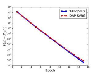
(a) $P(x)-P(x^{*})$ vs Epoch

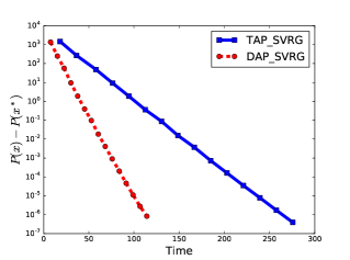
(b) $P(x)-P(x^{*})$ vs Time

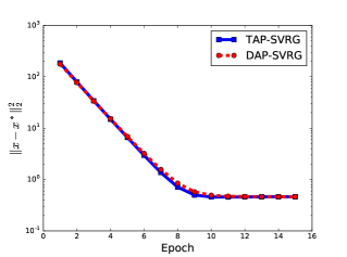
(c) $\|x-x^{*}\|_{2}^{2}$ vs Epoch

(d) $\|x-x^{*}\|_{2}^{2}$ vs Time

Figure 1: Performance of TAP-SVRG and DAP-SVRG for nuclear regularized objective. We evaluate the convergence of sub-optimality $P(x)-P(x^{*})$ and $\|x-x^{*}\|_{2}^{2}$ in terms of both epoch and time.

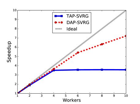
Figure 2: Time speedup when we increase the number of workers. The black dashed line denotes ideal speedup.

We also run TAP-SVRG and DAP-SVRG on distributed system and increase the number of workers from $1$ to $10$. Results in Figure 2 show that our DAP-SVRG enjoys near linear speedup. For TAP-SVRG method, its speedup is limited due to proximal mapping in the server. It is obvious that when the number of workers is greater than $4$, increasing workers does not help anymore.

5.2 Faster Convergence

In this section, compare our method with DAP-SGD [11]. We compare our DAP-SVRG method with TAP-SVRG, DAP-SGD constant and DAP-SGD decay. DAP-SGD constant denotes decoupled asynchronous proximal stochastic gradient descent method with constant learning rate, DAP-SGD decay denote decoupled asynchronous proximal stochastic gradient descent method with decreasing learning rate, where $\eta_{s}=\frac{\eta}{(s+1)^{\beta}}$. In our experiment, learning rate $\eta$ is tuned from $\{10^{-2},10^{-3},10^{-4}\}$, and $\beta$ is tuned from $\{0.1,0.3,0.5,0.7,0.9\}$. All experimental results are shown in Figure 3. At first iterations, DAP-SGD decay is faster than DAP-SVRG. Because of the variance of stochastic gradient, we have to reduce the learning rate for SGD method to guarantee convergence. DAP-SVRG’s learning rate keeps constant because the variance of stochastic gradient goes to zero. Thus, DAP-SVRG outperforms DAP-SGD decay after several epochs. It is clear that DAP-SVRG converges faster than DAP-SGD decay in terms of both epoch and time.

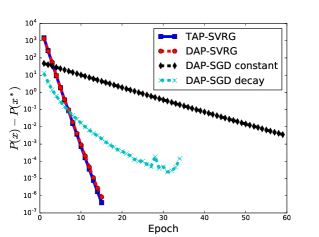
(a) $P(x)-P(x^{*})$ vs Epoch

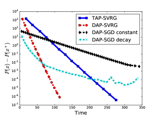
(b) $P(x)-P(x^{*})$ vs Time

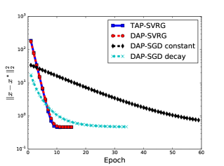
(c) $\|x-x^{*}\|_{2}^{2}$ vs Epoch

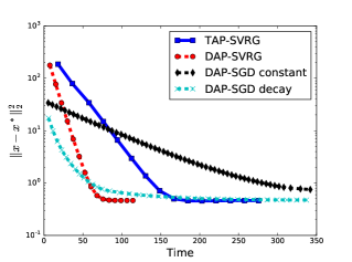
(d) $\|x-x^{*}\|_{2}^{2}$ vs Time

Figure 3: Performance of TAP-SVRG and DAP-SVRG for nuclear regularized objective. We evaluate the convergence of sub-optimality $P(x)-P(x^{*})$ and $\|x-x^{*}\|_{2}^{2}$ in terms of both epoch and time.

6 Conclusion

In this paper, we propose a decoupled asynchronous proximal stochastic variance reduced gradient descent method (DAP-SVRG). We use variance reduction technique, and accelerate the convergence rate of traditional asynchronous proximal stochastic gradient method. Additionally, by making workers do proximal mapping step, we relieve server from time-consuming operations. We further provide theoretical analysis of convergence property for DAP-SVRG, and it is proved to linear convergence when learning rate is constant. Experimental results also demonstrate our analysis.

Appendix A Proof of Lemma 1

Proof 1 (Lemma 1)

Because the definition of $u_{t}$ and $v_{t}$, we know that $\mathbb{E}u_{t}=\nabla f(x_{t})$ and $\mathbb{E}v_{t}=\nabla f(x_{d(t)})$, then we have:

$$\mathbb{E}\|v_{t}-\nabla f(x_{d(t)})\|_{2}^{2} = \mathbb{E}\|v_{t}-\nabla f(x_{d(t)})-u_{t}+u_{t}+\nabla f(x_{t})-\nabla f(x_{t})\|_{2}^{2}$$ (16)

$$\leq 2\mathbb{E}\|v_{t}-u_{t}-(\nabla f(x_{d}(t))-\nabla f(x_{t}))\|_{2}^{2}+2\mathbb{E}\|u_{t}-\nabla f(x_{t})\|_{2}^{2}$$

$$\leq 2\mathbb{E}\|\nabla f_{i}(x_{d(t)})-\nabla f_{i}(x_{t})\|_{2}^{2}+2\mathbb{E}\|u_{t}-\nabla f(x_{t})\|_{2}^{2}$$

$$\leq 2L^{2}\mathbb{E}\|x_{d(t)}-x_{t}\|_{2}^{2}+2\mathbb{E}\|u_{t}-\nabla f(x_{t})\|_{2}^{2}$$

$$\leq 2L^{2}\tau\sum\limits_{k=d(t)}^{t-1}\mathbb{E}\|x_{k+1}-x_{k}\|_{2}^{2}+2\mathbb{E}\|u_{t}-\nabla f(x_{t})\|_{2}^{2}$$

where the first inequality follows from the Lemma 3 in [18], the second inequality follows from this equation $\mathbb{E}\|\xi-\mathbb{E}\xi\|_{2}^{2}=\mathbb{E}\|\xi\|_{2}^{2}-\|\mathbb{E}\xi\|_{2}^{2}$, the third inequality follows from that $\nabla f_{i}(x)$ is Lipschitz continuous and the last inequality follows from the assumption that the maximum time delay has an upper bound $\tau$.

As per [11], the update of $x_{d(t)}^{\prime}$ in the worker can be represented as:

$$x_{d(t)}^{\prime} = \text{Prox}_{\eta,h}(x_{d_{t}}-\eta v_{t})$$ (17)

$$= \arg\min_{y}\frac{1}{2\eta}\|y-(x_{d(t)}-\eta v_{t})\|_{2}^{2}+h(y)$$

we define $\partial h(x)$ as the subgradient of $h(x)$, then we have:

$$\frac{1}{\eta}(x_{d(t)}-x_{d(t)}^{\prime})-v_{t}\in\partial h(x_{d(t)}^{\prime})$$ (18)

then the following inequality holds that:

$$\mathbb{E}\|v_{t}-\nabla f(x_{d(t)})\|_{2}^{2} \leq 2L^{2}\eta^{2}\tau\sum\limits_{k=d(t)}^{t-1}\mathbb{E}\|v_{k}+\partial h(x_{d(k)}^{\prime})\|_{2}^{2}+2\mathbb{E}\|u_{t}-\nabla f(x_{t})\|_{2}^{2}$$ (19)

$$= 2L^{2}\eta^{2}\tau\sum\limits_{k=d(t)}^{t-1}\mathbb{E}\|v_{k}+\partial h(x_{d(k)}^{\prime})-\nabla f(x_{d(k)})+\nabla f(x_{d(k)})\|_{2}^{2}$$

$$+2\mathbb{E}\|u_{t}-\nabla f(x_{t})\|_{2}^{2}$$

$$\leq 4L^{2}\eta^{2}\tau\sum\limits_{k=d(t)}^{t-1}\mathbb{E}\|\partial h(x_{d(k)}^{\prime})+\nabla f(x_{d(k)})\|_{2}^{2}$$

$$+4L^{2}\eta^{2}\tau\sum\limits_{k=d(t)}^{t-1}\mathbb{E}\|v_{k}-\nabla f(x_{d(k)})\|_{2}^{2}+2\mathbb{E}\|u_{t}-\nabla f(x_{t})\|_{2}^{2}$$

Follow the convergence proof in [3], we define $x_{d(t)}^{\prime}=x_{d(t)}-\eta G$, then we have $G=v_{t}+\partial h(x_{d(t)}^{\prime})$. Because $\nabla f(x)$ is Lipschitz continuous, then:

$$f(x_{d(t)}^{\prime}) \leq f(x_{d(t)})-\eta\nabla\left<f(x_{d(t)}),G\right>+\frac{L\eta^{2}}{2}\|G\|_{2}^{2}$$ (20)

$$\leq f(x_{d(t)})-\eta\nabla\left<f(x_{d(t)}),G\right>+\frac{\eta}{2}\|G\|_{2}^{2}$$

where we set $\eta\leq\frac{1}{L}$. Then $P(x_{d(t)}^{\prime})$ can be bounded in the following manner:

$$P(x_{d(t)}^{\prime}) = f(x_{d(t)}^{\prime})+h(x_{d(t)}^{\prime})$$ (21)

$$\leq f(x_{d(t)})-\eta\left<\nabla f(x_{d(t)}),G\right>+\frac{\eta}{2}\|G\|_{2}^{2}+h(x_{d(t)}^{\prime})$$

$$\leq f(z)-\left<\nabla f(x_{d(t)}),z-x_{d(t)}\right>-\frac{\mu}{2}\|z-x_{d(t)}\|_{2}^{2}-\eta\left<\nabla f(x_{d(t)}),G\right>$$

$$+\frac{\eta}{2}\|G\|_{2}^{2}+h(z)-\left<\partial h(x_{d(t)}^{\prime}),z-x_{d(t)}^{\prime}\right>$$

$$= f(z)-\left<\nabla f(x_{d(t)}),z-x_{d(t)}\right>-\frac{\mu}{2}\|z-x_{d(t)}\|_{2}^{2}-\eta\left<\nabla f(x_{d(t)}),G\right>$$

$$+\frac{\eta}{2}\|G\|_{2}^{2}+h(z)-\left<G-v_{t},z-x_{d(t)}+\eta G\right>$$

$$= P(z)-\left<\nabla f(x_{d(t)}),z-x_{d(t)}\right>-\frac{\mu}{2}\|z-x_{d(t)}\|_{2}^{2}-\eta\left<\nabla f(x_{d(t)}),G\right>$$

$$-\frac{\eta}{2}\|G\|_{2}^{2}-\left<G,z-x_{d(t)}\right>+\left<v_{t},z-x_{d(t)}\right>+\eta\left<v_{t},G\right>$$

where the first inequality comes form inequality (20), the second inequality comes from that both $f(x)$ and $h(x)$ are convex functions. We let $z=x_{d(t)}$, then the following inequality holds:

$$P(x_{d(t)}^{\prime})\leq P(x_{d(t)})-\frac{\eta}{2}\|G\|_{2}^{2}-\eta\left<G,\nabla f(x_{d(t)})-v_{t}\right>$$ (22)

Thus, $\mathbb{E}\|\partial h(x_{d(t)}^{\prime})+\nabla f(x_{d(t)})\|_{2}^{2}$ has an upper bound:

$$\mathbb{E}\|\partial h(x_{d(t)}^{\prime})+\nabla f(x_{d(t)})\|_{2}^{2} = \mathbb{E}\|\partial h(x_{d(t)}^{\prime})+\nabla f(x_{d(t)})-v_{t}+v_{t}\|_{2}^{2}$$ (23)

$$= \mathbb{E}\|v_{t}+\partial h(x_{d(t)}^{\prime})\|_{2}^{2}+\mathbb{E}\|v_{t}-\nabla f(x_{d(t)})\|_{2}^{2}$$

$$+2\mathbb{E}\left<v_{t}+\partial h(x_{d(t)}^{\prime}),\nabla f(x_{d(t)})-v_{t}\right>$$

$$\leq \mathbb{E}\|v_{t}-\nabla f(x_{d(t)})\|_{2}^{2}+\frac{2}{\eta}\mathbb{E}\left[P(x_{d(t)})-P(x_{d(t)}^{\prime})\right]$$

where the inequality follows from (22). Then, substituting (23) into (19) and adding both sides from $t=sm$ to $t=sm+m-1$, then we have:

$$\sum\limits_{t=sm}^{sm+m-1}\mathbb{E}\|v_{t}-\nabla f(x_{d(t)})\|_{2}^{2} \leq 8L^{2}\eta^{2}\tau^{2}\sum\limits_{t=sm}^{sm+m-1}\mathbb{E}\|v_{t}-\nabla f(x_{d(t)})\|_{2}^{2}$$ (24)

$$+8L^{2}\eta\tau^{2}\sum\limits_{t=sm}^{sm+m-1}\mathbb{E}[P(x_{t})-P(x_{t}^{\prime})]$$

$$+2\sum\limits_{t=sm}^{sm+m-1}\mathbb{E}\|u_{t}-\nabla f(x_{t})\|_{2}^{2}$$

Finally, the following inequality holds:

$$\sum\limits_{t=sm}^{sm+m-1}\mathbb{E}\|v_{t}-\nabla f(x_{d(t)})\|_{2}^{2} \leq \frac{8L^{2}\tau^{2}\eta}{1-8L^{2}\eta^{2}\tau^{2}}\sum\limits_{t=sm}^{sm+m-1}\mathbb{E}[P(x_{t})-P(x_{t}^{\prime})]$$ (25)

$$+\frac{2}{1-8L^{2}\eta^{2}\tau^{2}}\sum\limits_{t=sm}^{sm+m-1}\mathbb{E}\|u_{t}-\nabla f(x_{t})\|_{2}^{2}$$

Appendix B Proof of Theorem 2

Proof 2

Because the update rule $x_{t+1}-x_{t}=x_{d(t)}^{\prime}-x_{d(t)}$, then we have:

$$\mathbb{E}\|x_{t+1}-x^{*}\|_{2}^{2} = \mathbb{E}\|x_{t}-x^{*}-x_{d(t)}^{\prime}+x_{d(t)}\|_{2}^{2}$$ (26)

$$= \mathbb{E}\|x_{t}-x^{*}\|^{2}_{2}+\mathbb{E}\|x_{d(t)}^{\prime}-x_{d(t)}\|_{2}^{2}+2\mathbb{E}\left<x_{d(t)}^{\prime}-x_{d(t)},x_{t}-x^{*}\right>$$

$$= \mathbb{E}\|x_{t}-x^{*}\|^{2}_{2}+\underbrace{\mathbb{E}\|x_{d(t)}^{\prime}-x_{d(t)}\|_{2}^{2}+2\mathbb{E}\left<x_{d(t)}^{\prime}-x_{d(t)},x_{d(t)}-x^{*}\right>}_{Q_{1}}$$

$$+\underbrace{2\mathbb{E}\left<x_{d(t)}^{\prime}-x_{d(t)},x_{t}-x_{d(t)}\right>}_{Q_{2}}$$

Because $f(x)$ and $h(x)$ are both convex functions, then it holds that:

$$P(x^{*}) = f(x^{*})+h(x^{*})$$ (27)

$$\geq f(x_{d(t)})+\left<\nabla f(x_{d(t)}),x^{*}-x_{d(t)}\right>+h(x_{d(t)}^{\prime})+\left<\partial h(x_{d(t)}^{\prime}),x^{*}-x_{d(t)}^{\prime}\right>$$

$$\geq f(x_{d(t)}^{\prime})-\left<\nabla f(x_{d(t)}),x_{d(t)}^{\prime}-x_{d(t)}\right>-\frac{L}{2}\|x_{d(t)}^{\prime}-x_{d(t)}\|_{2}^{2}$$

$$+\left<\nabla f(x_{d(t)}),x^{*}-x_{d(t)}\right>+h(x_{d(t)}^{\prime})+\left<\frac{1}{\eta}(x_{d(t)}-x_{d(t)}^{\prime})-v_{t},x^{*}-x_{d(t)}^{\prime}\right>$$

$$\geq P(x_{d(t)}^{\prime})+\left<\nabla f(x_{d(t)})-v_{t},x^{*}-x_{d(t)}^{\prime}\right>+\frac{1}{\eta}\left<x_{d(t)}-x_{d(t)},x^{*}-x_{d(t)}\right>$$

$$+\frac{1}{2\eta}\|x_{d(t)}-x_{d(t)}^{\prime}\|_{2}^{2}$$

where the second inequality follows from that $\nabla f(x)$ is Lipschitz continuous, and the last inequality holds by setting $\eta\leq\frac{1}{L}$. Then take expectation on both sides, we have:

$$-\mathbb{E}[P(x_{d(t)}^{\prime})-P(x^{*})]+\underbrace{\mathbb{E}\left<v_{t}-\nabla f(x_{d(t)}),x^{*}-x_{d(t)}^{\prime}\right>}_{Q_{3}}\geq$$

$$+\frac{1}{\eta}\mathbb{E}\left<x_{d(t)}-x_{d(t)}^{\prime},x^{*}-x_{d(t)}\right>+\frac{1}{2\eta}\mathbb{E}\|x_{d(t)}-x_{d(t)}^{\prime}\|_{2}^{2}$$ (28)

Define $y=Prox_{\eta,h}\left(x_{d(t)}-\eta\nabla f(x_{d(t)})\right)$, and it is independent of sample $i$. then we have:

$$Q_{3} = \mathbb{E}\left<v_{t}-\nabla f(x_{d(t)}),x^{*}-y\right>+\mathbb{E}\left<v_{t}-\nabla f(x_{d(t)}),y-x_{d(t)}^{\prime}\right>$$ (29)

$$= \mathbb{E}\left<v_{t}-\nabla f(x_{d(t)}),y-x_{d(t)}^{\prime}\right>$$

$$\leq \mathbb{E}\|v_{t}-\nabla f(x_{d(t)})\|_{2}\|y-x_{d(t)}^{\prime}\|_{2}$$

$$\leq \eta\mathbb{E}\|v_{t}-\nabla f(x_{d(t)})\|_{2}^{2}$$

where the second equality follows from that $\mathbb{E}v_{t}=\nabla f(x_{d(t)})$, the first inequality follows from the Cauchy-Schwarz inequality, and the last inequality follows from the non-expansive property of proximal operator. Therefore, $Q_{1}$ is upper bounded as follows:

$$Q_{1} \leq -2\eta\mathbb{E}[P(x_{d(t)}^{\prime})-P(x^{*})]+2\eta^{2}\mathbb{E}\|v_{t}-\nabla f(x_{d(t)})\|_{2}^{2}$$ (30)

It is easy to know the upper bound of $Q_{2}$:

$$Q_{2} = 2\mathbb{E}\left<x_{d(t)}^{\prime}-x_{d(t)},x_{t}-x_{d(t)}\right>$$ (31)

$$\leq \mathbb{E}\|x_{d(t)}^{\prime}-x_{d(t)}\|_{2}^{2}+\mathbb{E}\|x_{t}-x_{d(t)}\|_{2}^{2}$$

$$= \mathbb{E}\|x_{d(t)}^{\prime}-x_{d(t)}\|_{2}^{2}+\mathbb{E}\|\sum\limits_{k=d(t)}^{t-1}(x_{k+1}-x_{k})\|_{2}^{2}$$

$$\leq \eta^{2}\mathbb{E}\|v_{t}+\partial h(x_{d(t)}^{\prime})\|_{2}^{2}+\tau\eta^{2}\sum\limits_{k=d(t)}^{t-1}\mathbb{E}\|v_{k}+\partial h(x_{d(k)}^{\prime})\|_{2}^{2}$$

$$\leq 2\eta^{2}\left(\mathbb{E}\|v_{t}-\nabla f(x_{d(t)})\|_{2}^{2}+\mathbb{E}\|\nabla f(x_{d(t)})+\partial h(x_{d(t)}^{\prime})\|_{2}^{2}\right)$$

$$+2\eta^{2}\tau\sum\limits_{k=d(t)}^{t-1}\left(\mathbb{E}\|v_{k}-\nabla f(x_{d(k)})\|_{2}^{2}+\mathbb{E}\|\nabla f(x_{d(k)})+\partial h(x_{d(k)}^{\prime})\|_{2}^{2}\right)$$

$$\leq 2\eta^{2}\left(2\mathbb{E}\|v_{t}-\nabla f(x_{d(t)})\|_{2}^{2}+\frac{2}{\eta}\mathbb{E}\left[P(x_{d(t)})-P(x_{d(t)}^{\prime})\right]\right)$$

$$+2\eta^{2}\tau\sum\limits_{k=d(t)}^{t-1}\left(2\mathbb{E}\|v_{k}-\nabla f(x_{d(k)})\|_{2}^{2}+\frac{2}{\eta}\mathbb{E}\left[P(x_{d(k)})-P(x_{d(k)}^{\prime})\right]\right)$$

where the second and last inequality use the assumption that maximum time delay is $\tau$, the last inequality follows from inequality (23).

Substituting $Q_{1}$ and $Q_{2}$ into inequality (26), and adding inequality (26) from $t=sm$ to $t=sm+m-1$, the following inequality holds:

$$\mathbb{E}\|x_{sm+m-1}-x^{*}\|_{2}^{2} \leq \mathbb{E}\|\tilde{x}_{s}-x^{*}\|_{2}^{2}-2\eta\sum\limits_{t=sm}^{sm+m-1}\mathbb{E}[P(x_{t})-P(x^{*})]$$ (32)

$$+(6\eta^{2}+4\eta^{2}\tau^{2})\sum\limits_{t=sm}^{sm+m-1}\mathbb{E}\|v_{t}-\nabla f(x_{d(t)})\|_{2}^{2}$$

$$+(6\eta+4\eta\tau^{2})\sum\limits_{t=sm}^{sm+m-1}\mathbb{E}\left[P(x_{t})-P(x_{t}^{\prime})\right]$$

where we use $\tilde{x}_{s}=x_{sm}$. Then assuming there is a very small positive constant $\varepsilon$ that satisfies $P(x_{t})-P(x_{t}^{\prime})\leq\varepsilon(P(x_{t})-P(x^{*}))$ and according to Lemma 1, we have:

$$\mathbb{E}\|x_{sm+m-1}-x^{*}\|_{2}^{2} \leq \mathbb{E}\|\tilde{x}_{s}-x^{*}\|_{2}^{2}-2\eta\sum\limits_{t=sm}^{sm+m-1}\mathbb{E}[P(x_{t})-P(x^{*})]$$ (33)

$$+\frac{8L^{2}\eta^{2}\tau\varepsilon(6\eta^{2}+4\eta^{2}\tau^{2})}{1-8L^{2}\eta^{2}\tau^{2}}\sum\limits_{t=sm}^{sm+m-1}\left[P(x_{t})-P(x^{*})\right]$$

$$+\frac{2(6\eta^{2}+4\eta^{2}\tau^{2})}{1-8L^{2}\eta^{2}\tau^{2}}\sum\limits_{t=sm}^{sm+m-1}\mathbb{E}\|u_{t}-\nabla f(x_{d(t)})\|_{2}^{2}$$

$$+(6\eta+4\eta\tau^{2})\varepsilon\sum\limits_{t=sm}^{sm+m-1}\mathbb{E}\left[P(x_{t})-P(x^{*})\right]$$

As per [22], we know

$$\|\tilde{x}_{s}-x^{*}\|_{2}^{2}\leq\frac{2}{\mu}\left[P(\tilde{x}_{s})-P(x^{*})\right]$$ (34)

$$\mathbb{E}\|u_{t}-\nabla f(x_{t})\|_{2}^{2}\leq 4L\left[P(x_{t})-P(x^{*})+P(\tilde{x})-P(x^{*})\right]$$ (35)

and

$$\sum\limits_{t=sm}^{sm+m-1}[P(x_{t})-P(x^{*})]\geq m[P(\tilde{x}_{s+1})-P(x^{*})]$$ (36)

finally we have:

$$\left(2\eta-\frac{8L^{2}\eta^{2}\tau\varepsilon(6\eta^{2}+4\eta^{2}\tau^{2})}{1-8L^{2}\eta^{2}\tau^{2}}-(6\eta+4\eta\tau^{2})\varepsilon-\frac{8L(6\eta^{2}+4\eta^{2}\tau^{2})}{1-8L^{2}\eta^{2}\tau^{2}}\right)m\mathbb{E}\left[P(\tilde{x}_{s+1})-P(x^{*})\right]$$

$$\leq\left(\frac{2}{\mu}+\frac{8L(6\eta^{2}+4\eta^{2}\tau^{2})m}{1-8L^{2}\eta^{2}\tau^{2}}\right)\mathbb{E}\left[P(\tilde{x}_{s})-P(x^{*})\right]$$ (37)

References

• [1] Léon Bottou. Large-scale machine learning with stochastic gradient descent. In Proceedings of COMPSTAT’2010, pages 177–186. Springer, 2010.
• [2] Aaron Defazio, Francis Bach, and Simon Lacoste-Julien. Saga: A fast incremental gradient method with support for non-strongly convex composite objectives. In Advances in Neural Information Processing Systems, pages 1646–1654, 2014.
• [3] L Vandenberghe EE236C. 6. proximal gradient method.
• [4] Cho-Jui Hsieh, Kai-Wei Chang, Chih-Jen Lin, S Sathiya Keerthi, and Sellamanickam Sundararajan. A dual coordinate descent method for large-scale linear svm. In Proceedings of the 25th international conference on Machine learning, pages 408–415. ACM, 2008.
• [5] Zhouyuan Huo and Heng Huang. Asynchronous stochastic gradient descent with variance reduction for non-convex optimization. arXiv preprint arXiv:1604.03584, 2016.
• [6] Martin Jaggi, Virginia Smith, Martin Takác, Jonathan Terhorst, Sanjay Krishnan, Thomas Hofmann, and Michael I Jordan. Communication-efficient distributed dual coordinate ascent. In Advances in Neural Information Processing Systems, pages 3068–3076, 2014.
• [7] Rie Johnson and Tong Zhang. Accelerating stochastic gradient descent using predictive variance reduction. In Advances in Neural Information Processing Systems, pages 315–323, 2013.
• [8] Jakub Konečnỳ, Jie Liu, Peter Richtárik, and Martin Takáč. ms2gd: Mini-batch semi-stochastic gradient descent in the proximal setting. arXiv preprint arXiv:1410.4744, 2014.
• [9] John Langford, Alexander Smola, and Martin Zinkevich. Slow learners are fast. arXiv preprint arXiv:0911.0491, 2009.
• [10] Mu Li, David G Andersen, Alex J Smola, and Kai Yu. Communication efficient distributed machine learning with the parameter server. In Advances in Neural Information Processing Systems, pages 19–27, 2014.
• [11] Yitan Li, Linli Xu, Xiaowei Zhong, and Qing Ling. Make workers work harder: Decoupled asynchronous proximal stochastic gradient descent. arXiv preprint arXiv:1605.06619, 2016.
• [12] Xiangru Lian, Yijun Huang, Yuncheng Li, and Ji Liu. Asynchronous parallel stochastic gradient for nonconvex optimization. In Advances in Neural Information Processing Systems, pages 2719–2727, 2015.
• [13] Ji Liu, Stephen J Wright, and Srikrishna Sridhar. An asynchronous parallel randomized kaczmarz algorithm. arXiv preprint arXiv:1401.4780, 2014.
• [14] Yucheng Low, Danny Bickson, Joseph Gonzalez, Carlos Guestrin, Aapo Kyrola, and Joseph M Hellerstein. Distributed graphlab: a framework for machine learning and data mining in the cloud. Proceedings of the VLDB Endowment, 5(8):716–727, 2012.
• [15] Atsushi Nitanda. Stochastic proximal gradient descent with acceleration techniques. In Advances in Neural Information Processing Systems, pages 1574–1582, 2014.
• [16] Augustus Odena. Faster asynchronous sgd. arXiv preprint arXiv:1601.04033, 2016.
• [17] Benjamin Recht, Christopher Re, Stephen Wright, and Feng Niu. Hogwild: A lock-free approach to parallelizing stochastic gradient descent. In Advances in Neural Information Processing Systems, pages 693–701, 2011.
• [18] Sashank J Reddi, Ahmed Hefny, Suvrit Sra, Barnabás Póczos, and Alex J Smola. On variance reduction in stochastic gradient descent and its asynchronous variants. In Advances in Neural Information Processing Systems, pages 2629–2637, 2015.
• [19] Lorenzo Rosasco, Silvia Villa, and Bang Công Vũ. Convergence of stochastic proximal gradient algorithm. arXiv preprint arXiv:1403.5074, 2014.
• [20] Shai Shalev-Shwartz and Tong Zhang. Stochastic dual coordinate ascent methods for regularized loss. The Journal of Machine Learning Research, 14(1):567–599, 2013.
• [21] Martin Takác, Peter Richtárik, and Nathan Srebro. Distributed mini-batch sdca. arXiv preprint arXiv:1507.08322, 2015.
• [22] Lin Xiao and Tong Zhang. A proximal stochastic gradient method with progressive variance reduction. SIAM Journal on Optimization, 24(4):2057–2075, 2014.
• [23] Tianbao Yang. Trading computation for communication: Distributed stochastic dual coordinate ascent. In Advances in Neural Information Processing Systems, pages 629–637, 2013.
• [24] Ruiliang Zhang and James Kwok. Asynchronous distributed admm for consensus optimization. In Proceedings of the 31st International Conference on Machine Learning (ICML-14), pages 1701–1709, 2014.
• [25] Ruiliang Zhang, Shuai Zheng, and James T Kwok. Fast distributed asynchronous sgd with variance reduction. arXiv preprint arXiv:1508.01633, 2015.
• [26] Wei Zhang, Suyog Gupta, Xiangru Lian, and Ji Liu. Staleness-aware async-sgd for distributed deep learning. arXiv preprint arXiv:1511.05950, 2015.
• [27] Shen-Yi Zhao and Wu-Jun Li. Fast asynchronous parallel stochastic gradient descent: A lock-free approach with convergence guarantee. 2016.
• [28] Wenliang Zhong and James Tin-Yau Kwok. Accelerated stochastic gradient method for composite regularization. In AISTATS, pages 1086–1094, 2014.