Central Runge-Kutta discontinuous Galerkin methods for the special relativistic hydrodynamics

Abstract

This paper developes Runge-Kutta $P^{K}$-based central discontinuous Galerkin (CDG) methods with WENO limiter to the one- and two-dimensional special relativistic hydrodynamical (RHD) equations, $K=1,2,3$. Different from the non-central DG methods, the Runge-Kutta CDG methods have to find two approximate solutions defined on mutually dual meshes. For each mesh, the CDG approximate solutions on its dual mesh are used to calculate the flux values in the cell and on the cell boundary so that the approximate solutions on mutually dual meshes are coupled with each other, and the use of numerical flux may be avoided. The WENO limiter is adaptively implemented via two steps: the “troubled” cells are first identified by using a modified TVB minmod function, and then the WENO technique is used to locally reconstruct new polynomials of degree $(2K+1)$ replacing the CDG solutions inside the “troubled” cells by the cell average values of the CDG solutions in the neighboring cells as well as the original cell averages of the “troubled” cells. Because the WENO limiter is only employed for finite “troubled” cells, the computational cost can be as little as possible. The accuracy of the CDG without the numerical dissipation is analyzed and calculation of the flux integrals over the cells is also addressed. Several test problems in one and two dimensions are solved by using our Runge-Kutta CDG methods with WENO limiter. The computations demonstrate that our methods are stable, accurate, and robust in solving complex RHD problems.

%֮ǰ

1 Introduction

Relativistic fluid widely appears in nuclear physics, astrophysics, plasma physics, and other fields. For example, in the physical phenomena such as the formation of neutron stars and black holes and the high-speed jet, the local fluid velocity may be close to the speed of light, at this time the relativistic effect can not be neglected and the relativistic fluid dynamics (RHD) is needed. Because the RHD equations are more complicated, their theoretical analysis is impractical so that conversely numerical simulation has become a primary and powerful way to study and understand the physical mechanisms in the RHDs.

The pioneering numerical work may date back to the finite difference code via artificial viscosity for the spherically symmetric general RHD equations in the Lagrangian coordinate [31, 32]. Wilson first attempted to solve multi-dimensional RHD equations in the Eulerian coordinate by using the finite difference method with the artificial viscosity technique [45]. Since 1990s, the numerical study of the RHDs began to attract considerable attention, and various modern shock-capturing methods with an exact or approximate Riemann solver have been developed for the RHD equations, the readers are referred to the early review articles [30, 44]. Some examples on existing methods, which are extensions of Godunov type shock capturing methods, are the upwind schemes based on local linearization [16, 17], the two shock spproximation solvers [1, 12, 34], flux-vector splitting scheme [14], HLL (Harten-Lax-van Leer) schemes [39, 15], HLLC (Harten-Lax-van Leer-Contact) scheme [33], non-oscillatory essentially (ENO) schemes [13, 56], and kinetic schemes [53, 21] and so on. Recently the second author and his co-workers developed adaptive moving mesh method [18], derived the second-order accurate generalized Riemann problem (GRP) methods for the one- and two-dimensional RHD equations [54, 55], and the finite volume local evolution Galerkin scheme for two-dimensional RHD equations [46]. Later, the third-order accurate GRP scheme in [52] was extended to the one-dimensional RHD equations [51], and the direct Eulerian GRP scheme was developed for the spherically symmetric general relativistic hydrodynamics [47]. The physical-constraints-preserving (PCP) schemes were also studied for the special RHD equations recently. The high-order accurate PCP finite difference weighted essentially non-oscillatory (WENO) schemes and discontinuous Galerkin (DG) methods were proposed in [48, 50, 35]. Moreover, the set of admissible states and the PCP schemes of the ideal relativistic magnetohydrodynamics was studied for the first time in [49], where the importance of divergence-free fields was revealed in achieving PCP methods especially.

The DG methods have been rapidly developed in recent decades and has become a kind of important methods in computational fluid dynamics. They are easy to achieve high order accuracy, suitable for parallel computing, and adapt to complex domain boundary. The DG method was first developed by Reed and Hill [37] to solve steady-state scalar linear hyperbolic equation but it had not been widely used. A major development of the DG method was carried out in a series of papers [8, 7, 6, 4, 10], where the DG spatial approximation was combined with explicit Runge-Kutta time discretization to develop Runge-Kutta DG (RKDG) methods and a general framework of DG methods was established for the nonlinear equation or system. After that, the RKDG methods began to get a wide range of research and application, such as the Euler equations [43, 3, 38], Maxwell equations [5], nonlinear Dirac equations [40] etc. Moreover, the DG methods have also been used to solve other partial differential equations, such as convection-diffusion type equation or system [2, 9] and Hamilton-Jacobi equation [19, 23, 26] etc. The readers are referred to the review article [11]. The Runge-Kutta CDG methods [28] were developed by combing RKDG methods and central scheme [27] and found two approximate solutions defined on mutually dual meshes. Although two approximate solutions are redundant, the numerical flux may be avoided due to the use of the solution on the dual mesh to calculate the flux at the cell interface. It is one of the advantages of the central scheme. Because the Runge-Kutta CDG methods can be considered as a variant of RKDG methods, they keep many advantages of RKDG methods, such as compact stencil and parallel implementation etc. Moreover, the Runge-Kutta CDG methods allow a larger CFL number than RKDG methods and reduce numerical oscillations for some problems. Up to now, the Runge-Kutta CDG methods have also been used to solve the Euler equations [28] and the ideal magneto-hydrodynamical equations [25, 24] and so on.

A deficiency of the RKDG methods is that when the strong discontinuity appears in the solution, the numerical oscillations should be suppressed after each Runge-Kutta inner stage or after some complete Runge-Kutta steps by using the nonlinear limiter, which is a commonly used technique of the modern shock-capturing methods for hyperbolic conservation laws. The commonly used limiter is the minmod limiter, which limits the slope of solution such that the values of limited solution in the cell falls in the certain interval determined by the cell average values of neighboring cells. The minmod limiter has good robustness but becomes only first-order accurate near extreme points. The modified TVB minmod limiter is given in [7] and applied to the RKDG methods. It does not limit the solution near extreme points by choosing a parameter $M$, thus the accuracy of RKDG methods is not destroyed near the extreme point. In general, for nonlinear equation, the parameter is dependent on the problem, and the accuracy of $P^{K}$-based RKDG methods for $K\geq 3$ may still be destroyed because more than three of the higher order moments will be set to zero in the modified TVB minmod limiter. Besides those commonly used limiters, some other limiters are porposed, such as the moment based limiters [3] and its improvement [20] etc. Those limiters may suppress numerical oscillations near the discontinuity, however, the accuracy of RKDG methods may be reduced in the some region.

In the modern shock-capturing methods, the ENO and WENO methods are more robust than the slope limiters especially for high order schemes and have been widely used,see the review article [41]. An attempt was made to use them as limiters for the DG methods [36, 62, 61]. The WENO limiter first identifies the “troubled” cells by using a modified TVB minmod function, and then new polynomials inside the “troubled” cells are locally reconstructed to replace the DG solutions by using the WENO technique based on the cell average values of the DG solutions in the neighboring cells as well as the original cell averages of the “troubled” cells. It is only employed for finite “troubled” cells, so the computational cost can be as little as possible.

This paper proposes the Runge-Kutta $P^{K}$-based CDG methods with WENO limiter for the one- and two-dimensional special RHD equations, $K=1,2,3$. It is organized as follows. Section 2 introduces the system of special RHD equations. Section 3 proposes Runge-Kutta $P^{K}$-based CDG methods with WENO limiter. Section 4 gives some discussions of the Runge-Kutta CDG methods. Section 5 gives several numerical examples to verify the accuracy robustness, and effectiveness of the proposed Runge-Kutta CDG methods. Concluding remarks are presented in Section 6.

2 Special RHD equations

This section introduces the governing equations of the special relativistic hydrodynamics (RHD). Similar to the non-relativistic case, the special RHD equations may be established by the laws of local baryon number conservation and energy-momentum conservation [22] and cast into the following covariant form

$$\begin{cases}\partial_{\alpha}(\rho u^{\alpha})=0,\\ \partial_{\alpha}\Big{(}\rho hu^{\alpha}u^{\beta}+pg^{\alpha\beta}\Big{)}=0,\end{cases}$$ (2.1)

where the Greek indices $\alpha$ and $\beta$ run from 0 to 3, $\partial_{\alpha}=\partial_{x^{\alpha}}$ stands for the covariant derivative, $g^{\alpha\beta}$ denotes the metric tensor and is restricted to the Minkowski tensor throughout the paper, i.e. $\big{(}g^{\alpha\beta}\big{)}_{4\times 4}=\mbox{diag}\{-1,1,1,1\}$, $\rho$, $u^{\alpha}$ and $p$ denote the rest-mass density, four-velocity vector, and pressure, respectively, and $h$ is the specific enthalpy defined by

$$h=1+e+\displaystyle{\frac{p}{\rho}},$$ (2.2)

here $e$ denotes the specific internal energy. For the sake of convenience, units in which the speed of light is equal to one will be used so that $x^{\alpha}=(t,x_{1},x_{2},x_{3})^{T}$ and $u^{\alpha}=\gamma(1,v_{1},v_{2},v_{3})^{T}$, where $\gamma=1/\sqrt{1-v^{2}}$ is the Lorentz factor and $v:=\sqrt{v_{1}^{2}+v_{2}^{2}+v_{3}^{2}}$ is the size of fluid velocity.

In order to close the above system (2.1), an equation of state (EOS) for the thermodynamical variables

$$p=p(\rho,e),$$ (2.3)

is needed. For example, the EOS for an ideal gas can be expressed in the $\Gamma$-law form

$$p=(\Gamma-1)\rho e,$$ (2.4)

where $\Gamma$ is the adiabatic index, taken as 5/3 for the mildly relativistic case and 4/3 for the ultra-relativistic case.

The covariant form of special RHD equations (2.1) is usually written into a time-dependent system of conservation laws in the laboratory frame as follows

$$\frac{\partial\mbox{\boldmath\small$U$}}{\partial t}+\sum^{d}_{i=1}\frac{\partial\mbox{\boldmath\small$F$}_{i}(\mbox{\boldmath\small$U$})}{\partial x_{i}}=0,$$ (2.5)

where $U$ is conservative variable vector and $\mbox{\boldmath\small$F$}_{i}$ denotes and the flux vector in the $x_{i}$ direction, $i=1,\cdots,d$. For example, in the case of $d=3$, the detailed expressions of $U$ and $\mbox{\boldmath\small$F$}_{i}$ are

$$\begin{aligned} \mbox{\boldmath\small$U$}=&\Big{(}D,m_{1},m_{2},m_{3},E\Big{)}^{T},\\ \mbox{\boldmath\small$F$}_{1}=&\Big{(}Dv_{1},m_{1}v_{1}+p,m_{2}v_{1},m_{3}v_{1},m_{1}\Big{)}^{T},\\ \mbox{\boldmath\small$F$}_{2}=&\Big{(}Dv_{2},m_{1}v_{2},m_{2}v_{2}+p,m_{3}v_{2},m_{2}\Big{)}^{T},\\ \mbox{\boldmath\small$F$}_{3}=&\Big{(}Dv_{3},m_{1}v_{3},m_{2}v_{3},m_{3}v_{3}+p,m_{3}\Big{)}^{T},\end{aligned}$$ (2.6)

here $D=\rho\gamma$, $m_{i}=\rho h\gamma^{2}v_{i}$ , and $E=\rho h\gamma^{2}-p$ denote the mass, $x_{i}$-momentum, and energy densities relative to the laboratory frame, respectively.

The formal structure of (2.5) is identical to that of the three-dimensional non-relativistic Euler equations. The momentum equations in (2.5) are only with a Lorentz-contracted momentum density replacing $\rho v_{i}$ in the non-relativistic Euler equations. When the fluid velocity is small ($v\ll 1=c$) and the velocity of the internal (microscopic) motion of the fluid particles is small, the RHD equations (2.5) reduce to the non-relativistic Euler equations. The system (2.5) also satisfies the properties of the rotational invariance and the homogeneity as well as the hyperbolicity in time when (2.4) is used, see [59]. However, in comparison to the non-relativistic Euler equations, a strong coupling between the hydrodynamic equations is introduced and additional numerical difficulties are posed due to the relations between the laboratory quantities (the mass density $D$, the momentum density $m_{i}$, and the energy density $E$) and the quantities in the local rest frame (the mass density $\rho$, and the fluid velocity $v_{i}$, the internal energy density $e$). Especially, the flux $\mbox{\boldmath\small$F$}_{i}$ in (2.5) can not be formulated in an explicit form of the conservative vector $U$ and the physical constraints $E\geq D$, $\rho>0$, $p>0$, and $v<1$ have to be fulfilled. Thus, in practical computations of the system (2.5) by using the shock-capturing methods, the primitive variable vector $\mbox{\boldmath\small$V$}=(\rho,v_{1},\cdots,v_{d},p)^{T}$ has to be first recovered from the known conservative vector $\mbox{\boldmath\small$U$}=(D,m_{1},\cdots,m_{d},E)^{T}$ at each time step by numerically solving a nonlinear pressure equation such as

$$E+p=D\gamma+\displaystyle\frac{\Gamma}{\Gamma-1}p\gamma^{2},$$ (2.7)

where $\gamma=(1-|\mbox{\boldmath\small$m$}|^{2}/(E+p)^{2})^{-1/2}$. Any standard root-finding algorithm, e.g. Newton’s iteration, may be used to solve (2.7) to get the pressure, and then $\gamma$, $\rho$, $e$, $h$, and $v_{i}$ in order, the readers are referred to [60] for the choice of initial guess.

3 Runge-Kutta CDG methods

This section gives the Runge-Kutta central DG methods for the hyperbolic conservation laws. For the sake of simplicity, one-dimensional scalar equation

$$\frac{\partial u(x,t)}{\partial t}+\frac{\partial f(u(x,t))}{\partial x}=0,\quad x\in\Omega,$$ (3.1)

is taken as an example to introduce the Runge-Kutta CDG methods [28]. Similar to the non-central RKDG methods, the Runge-Kutta CDG methods also employ the discontinuous Galerkin finite element in the spatial discretization and the explicit Runge-Kutta method for the time discretization. Their difference between them is that Runge-Kutta CDG methods need two mutually dual meshes, see the one-dimensional schematic diagram in Fig. 3.1 for the mesh $\{C_{j}=(x_{j-\frac{1}{2}},x_{j+\frac{1}{2}}),\forall j\in\mathbb{Z}\}$ and its dual mesh $\{D_{j+\frac{1}{2}}=(x_{j},x_{j+1}),\forall j\in\mathbb{Z}\}$.

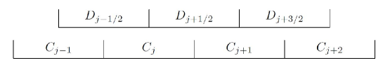
Figure 3.1: Schematic diagram of mutually dual meshes for the 1D Runge-Kutta CDG methods.

The aim of Runge-Kutta CDG methods is to find two approximate solutions $u^{C}_{h}(x,t)$ and $u^{D}_{h}(x,t)$ such that at any time $t\in(0,T]$, they belong to the following finite spaces respectively

$$\mathcal{V}^{C}:=\left\{v(x)\in L^{1}(\Omega)|v(x)\in\mathbb{P}^{K}(C_{j}),\mbox{}~{}x\in C_{j}\subset\Omega,\forall j\right\},$$

$$\mathcal{V}^{D}:=\left\{w(x)\in L^{1}(\Omega)|~{}w(x)\in\mathbb{P}^{K}(D_{j+\frac{1}{2}}),\mbox{ }~{}x\in D_{j+\frac{1}{2}}\subset\Omega,\forall j\right\}.$$

Consider the CDG scheme for the approximate solution $u^{C}_{h}$. Multiplying (3.1) by the test function $v(x)\in\mathbb{P}^{K}(C_{j})$ and integrating it over the cell $C_{j}$ by parts gives

$$\frac{d}{dt}\int_{C_{j}}uvdx=\int_{C_{j}}f(u)\frac{\partial v}{\partial x}dx-f\big{(}u(x_{j+\frac{1}{2}},t)\big{)}v(x_{j+\frac{1}{2}})+f\big{(}u(x_{j-\frac{1}{2}},t)\big{)}v(x_{j-\frac{1}{2}}).$$ (3.2)

If replacing $u$ at the left- and right-hand sides of (3.2) with the approximate solution $u^{C}_{h}$ and $u^{D}_{h}$, respectively, then one has

$$\frac{d}{dt}\int_{C_{j}}u^{C}_{h}vdx= \frac{1}{\tau_{max}}\int_{C_{j}}(u^{D}_{h}-u^{C}_{h})v(x)dx+\int_{C_{j}}f(u^{D}_{h})\frac{\partial v}{\partial x}dx$$

$$- f\big{(}u^{D}_{h}(x_{j+\frac{1}{2}},t)\big{)}v(x_{j+\frac{1}{2}})+f\big{(}u^{D}_{h}(x_{j-\frac{1}{2}},t)\big{)}v(x_{j-\frac{1}{2}}),$$ (3.3)

where the first term at the right-hand side of (3.3) denotes the numerical dissipation term borrowing from the central scheme [27], and $\tau_{max}$ denotes the maximum time step size allowed by the CFL condition. Because the approximate solution $u^{D}_{h}$ is continuous at the boundary of cell $C_{j}$, the fluxes $f(u(x_{j\pm\frac{1}{2}},t))$ may be directly evaluated and thus numerical flux is not required in the CDG methods.

If using $\phi_{j}^{(l)}(x)$, $l=0,...K$, to denote a basis of the space $\mathbb{P}^{K}(C_{j})$, then $u^{C}_{h}$ may be expressed as

$$u^{C}_{h}(x,t)=\sum_{l=0}^{K}u^{C,(l)}_{j}(t)\phi_{j}^{(l)}(x)=:u^{C}_{j}(x,t),\quad~{}x\in C_{j}.$$

Replacing $v(x)$ in (3.3) with the basis function $\phi_{j}^{(\ell)}(x)$ and using the numerical quadrature with $q$ points to calculate the integral with flux $f(u)$ gives the semi-discrete scheme for $u^{C}_{h}$ as follows

$$\sum_{l=0}^{K}\big{(}\int_{C_{j}}\phi_{j}^{(\ell)}(x)\phi_{j}^{(l)}(x)dx\big{)}\frac{du^{C,(l)}_{j}}{dt}=\frac{1}{\tau_{max}}\int_{C_{j}}(u^{D}_{h}-u^{C}_{h})\phi_{j}^{(\ell)}(x)dx$$

$$-f\big{(}u^{D}_{h}(x_{j+\frac{1}{2}},t)\big{)}\phi_{j}^{(\ell)}(x_{j+\frac{1}{2}})+f\big{(}u^{D}_{h}(x_{j-\frac{1}{2}},t)\big{)}\phi_{j}^{(\ell)}(x_{j-\frac{1}{2}})$$

$$+h_{j}\sum_{m=1}^{q}\omega_{m}^{C}f\big{(}u^{D}_{h}(x^{C}_{m},t)\big{)}\frac{\partial}{\partial x}\phi_{j}^{(\ell)}(x_{m}^{C}),\quad\ell=0,1,\cdots,K,$$ (3.4)

where $h_{j}=x_{j+\frac{1}{2}}-x_{j-\frac{1}{2}}$, and $x^{C}_{m}$ and $\omega^{C}_{m}$ denote the point and weight for the numerical integration over the cell $C_{j}$, $m=1,\cdots,q$. It needs to be pointed out that the first term at the right-hand side of (3.4) is an integral of piecewise polynomial and may be exactly calculated.

The semi-discrete scheme for the approximate solution $u^{D}_{h}$ may be similarly derived. If choosing a basis of the space $\mathbb{P}^{K}(D_{j+\frac{1}{2}})$ as $\{\varphi_{j+\frac{1}{2}}^{(l)}(x),~{}l=0,...K\}$, then the semi-discrete scheme for $u^{D}_{h}$ is given as follows

$$\sum_{l=0}^{K}\big{(}\int_{D_{j+\frac{1}{2}}}\varphi_{j+\frac{1}{2}}^{(\ell)}(x)\varphi_{j+\frac{1}{2}}^{(l)}(x)dx\big{)}\frac{du^{D,(l)}_{j+\frac{1}{2}}}{dt}=\frac{1}{\tau_{max}}\int_{D_{j+\frac{1}{2}}}(u^{C}_{h}-u^{D}_{h})\varphi_{j+\frac{1}{2}}^{(\ell)}(x)dx$$

$$-f\big{(}u^{C}_{h}(x_{j+1},t)\big{)}\varphi_{j+\frac{1}{2}}^{(\ell)}(x_{j+1})+f\big{(}u^{C}_{h}(x_{j},t)\big{)}\varphi_{j+\frac{1}{2}}^{(\ell)}(x_{j})$$

$$+h_{j+\frac{1}{2}}\sum_{m=1}^{q}\omega_{m}^{D}f\big{(}u^{C}_{h}(x^{D}_{m},t)\big{)}\frac{\partial}{\partial x}\varphi_{j+\frac{1}{2}}^{(\ell)}(x_{m}^{D}),\quad\ell=0,1,\cdots,K.$$ (3.5)

Remark 3.1

If $f(u)=u$, then two approximate solutions satisfy [29]

$$\frac{1}{2}\frac{d}{dt}\int_{\Omega}\big{(}(u_{h}^{C})^{2}+(u_{h}^{D})^{2}\big{)}dx=-\frac{1}{\tau_{max}}\int_{\Omega}(u_{h}^{C}-u_{h}^{D})^{2}dx\leq 0.$$ (3.6)

It can be known, that is why the term $\frac{1}{\tau_{max}}\int_{C_{j}}(u^{D}_{h}-u^{C}_{h})v(x)dx$ in (3.3) is called as numerical dissipation.

Remark 3.2

It is worth noting that the flux within the cell $C_{j}$ in (3.3) is evaluated by using $u^{D}_{h}$, but the approximate solution $u^{D}_{h}$ is not continuous at $x_{j}$, thus before using the numerical integration to evaluate the integral of flux over $C_{j}$ in (3.3), one has to split it into two parts

$$\int_{x_{j-\frac{1}{2}}}^{x_{j+\frac{1}{2}}}f(u^{D}_{h})\frac{\partial v}{\partial x}dx=\int_{x_{j-\frac{1}{2}}}^{x_{j}}f(u^{D}_{j-\frac{1}{2}})\frac{\partial v}{\partial x}dx+\int_{x_{j}}^{x_{j+\frac{1}{2}}}f(u^{D}_{j+\frac{1}{2}})\frac{\partial v}{\partial x}dx,$$ (3.7)

and then use Gaussian quadrature with $K+1$ points to calculate two integrals at the right-hand side of the above equation. The flux integral in (3.5) should be similarly treated. Section 4.2 will give a further discussion on the evaluation of such flux integral.

Both semi-discrete CDG schemes (3.4) and (3.5) may be cast into the following abstract form

$$\frac{\partial\mbox{\boldmath\small$U$}}{\partial t}=\mbox{\boldmath\small$L$}(\mbox{\boldmath\small$U$}),$$

which is a nonlinear system of ordinary differential equation of $U$ with respect to $t$, and thus the time derivatives may be further approximated to give the fully-discrete CDG methods may be derived for the degrees of freedom or the moments by using the third-order accurate TVD (total variation diminishing) Runge-Kutta method [42]

$$\begin{aligned} \mbox{\boldmath\small$U$}^{(1)}=&\mbox{\boldmath\small$U$}^{n}+\Delta t_{n}\mbox{\boldmath\small$L$}(\mbox{\boldmath\small$U$}^{n}),\\ \mbox{\boldmath\small$U$}^{(2)}=&\frac{3}{4}\mbox{\boldmath\small$U$}^{n}+\frac{1}{4}\big{(}\mbox{\boldmath\small$U$}^{(1)}+\Delta t_{n}\mbox{\boldmath\small$L$}(\mbox{\boldmath\small$U$}^{(1)})\big{)},\\ \mbox{\boldmath\small$U$}^{n+1}=&\frac{1}{3}\mbox{\boldmath\small$U$}^{n}+\frac{2}{3}\big{(}\mbox{\boldmath\small$U$}^{(2)}+\Delta t_{n}\mbox{\boldmath\small$L$}(\mbox{\boldmath\small$U$}^{(2)})\big{)},\end{aligned}$$ (3.8)

or the fourth-order accurate non-TVD Runge-Kutta method

$$\begin{aligned} &\mbox{\boldmath\small$U$}^{(1)}=\mbox{\boldmath\small$U$}^{n}+\frac{1}{2}\Delta t_{n}\mbox{\boldmath\small$L$}(\mbox{\boldmath\small$U$}^{n}),\\ &\mbox{\boldmath\small$U$}^{(2)}=\mbox{\boldmath\small$U$}^{n}+\frac{1}{2}\Delta t_{n}\mbox{\boldmath\small$L$}(\mbox{\boldmath\small$U$}^{(1)}),\\ &\mbox{\boldmath\small$U$}^{(3)}=\mbox{\boldmath\small$U$}^{n}+\Delta t_{n}\mbox{\boldmath\small$L$}(\mbox{\boldmath\small$U$}^{(2)}),\\ &\mbox{\boldmath\small$U$}^{n+1}=\frac{1}{3}\big{(}\mbox{\boldmath\small$U$}^{(1)}+2\mbox{\boldmath\small$U$}^{(2)}+3\mbox{\boldmath\small$U$}^{(3)}-\mbox{\boldmath\small$U$}^{n}+\frac{1}{2}\Delta t_{n}\mbox{\boldmath\small$L$}(\mbox{\boldmath\small$U$}^{(3)})\big{)}.\end{aligned}$$ (3.9)

and so on.

As mentioned above, $\tau_{max}$ is determined by using the CFL condition. After determining $\tau_{max}=\tau_{n}$ at $t=t_{n}$, the practical time stepsize $\Delta t_{n}$ should satisfy $0<\Delta t_{n}\leq\tau_{n}$. If denoting $\theta=\Delta t_{n}/\tau_{n}$, then $\theta\in(0,1]$. For hyperbolic equations, $\Delta t_{n}$ may usually be taken as $\tau_{n}$, that is, $\theta=1$.

Although the Runge-Kutta CDG methods are only introduced for one-dimensional scalar conservation law, their extension to one-dimensional RHD equations and two-dimensional rectangular mesh is easy and direct. Similar to the non-central RKDG methods, the limiting procedure is necessary for the Runge-Kutta CDG methods when the solution contains strong discontinuity. The WENO limiting procedure in Section 3.3 of [60] may be directly and independently applied to the solutions $u^{C}_{h}$ and $u^{D}_{h}$ of Runge-Kutta CDG methods by the following two steps:

• identify the “troubled” cells in the meshes $\{C_{j}\}$ and $\{D_{j+1/2}\}$, namely, those cells which might need the limiting procedure,

• replace the CDG solution polynomials $u^{C}_{h}$ and $u^{D}_{h}$ in those “troubled” cells with WENO reconstructed polynomials of degree $(2K+1)$, denoted by $u^{C,WENO}_{h}$ and $u^{D,WENO}_{h}$, which maintain the original cell averages (conservation) and the accuracy, but have less numerical oscillation.

In order to save the length of paper, those details are omitted here.

4 Some discussions of Runge-Kutta CDG methods

In comparison to the non-central RKDG methods, the Runge-Kutta CDG methods has an additional numerical dissipation term. Remark 3.1 has shown that such dissipation term is important for the $L^{2}$ stability of CDG methods. This section discusses the accuracy of Runge-Kutta CDG methods without the numerical dissipation in order to understand that the impact of numerical dissipation term on the accuracy of CDG methods. Furthermore, this section will also discuss the calculation of flux integral over the cell mentioned in Remark 3.2.

4.1 Accuracy of CDG methods without numerical dissipation

The semi-discrete version of Runge-Kutta CDG methods without numerical dissipation can be written as follows

$$\begin{aligned} \frac{d}{dt}\int_{C_{j}}u^{C}_{h}vdx=&\int_{C_{j}}f(u^{D}_{h})\frac{\partial v}{\partial x}dx-f\big{(}u^{D}_{h}(x_{j+\frac{1}{2}},t)\big{)}v(x_{j+\frac{1}{2}})\\ &+f\big{(}u^{D}_{h}(x_{j-\frac{1}{2}},t)\big{)}v(x_{j-\frac{1}{2}}),\quad\forall v(x)\in\mathbb{P}^{K}(C_{j}),\\ \frac{d}{dt}\int_{D_{j+\frac{1}{2}}}u^{D}_{h}wdx=&\int_{D_{j+\frac{1}{2}}}f(u^{C}_{h})\frac{\partial w}{\partial x}dx-f\big{(}u^{C}_{h}(x_{j+1},t)\big{)}w(x_{j+1})\\ &+f\big{(}u^{C}_{h}(x_{j},t)\big{)}w(x_{j}),\quad\forall w(x)\in\mathbb{P}^{K}(D_{j+\frac{1}{2}}).\end{aligned}$$ (4.1)

The accuracy of $P^{1}$-based CDG methods without numerical dissipation is first discussed here by using the Fourier method similar to [57, 58]. Use (4.1) to solve the scalar equation

$$u_{t}+u_{x}=0,\quad x\in[0,2\pi],$$ (4.2)

subject to the initial condition $u(x,0)=\sin(x)$.

For the CDG solution on the mesh $\{C_{j}\}$. As shown in Fig. 4.2, for the sake of convenience, the degrees of freedom are chosen as the function values at $2N$ points distributed with equal distance

$$u^{C}_{j-\frac{1}{4}},~{}u^{C}_{j+\frac{1}{4}},~{}j=1,\cdots,N,$$

instead of all order moments $\{u^{C,(l)}_{j}(t)\}$.

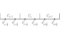
Figure 4.2: Schematic diagram of degrees of freedom.

Within the cell $C_{j}$, the solution $u^{C}_{j}(x,t)$ may be expressed as

$$u^{C}_{j}(x,t)=u^{C}_{j-\frac{1}{4}}(t)\phi_{j-\frac{1}{4}}(x)+u^{C}_{j+\frac{1}{4}}(t)\phi_{j+\frac{1}{4}}(x),$$

where $\phi_{j\pm\frac{1}{4}}(x)$ denote the basis functions, given by

$$\phi_{j-\frac{1}{4}}(x)=\frac{1}{2}-\frac{2(x-x_{j})}{h},\quad\phi_{j+\frac{1}{4}}(x)=\frac{1}{2}+\frac{2(x-x_{j})}{h}.$$

Similarly, within the cell $D_{j+\frac{1}{2}}$, the solution $u^{D}_{j+\frac{1}{2}}(x,t)$ may be written as follows

$$u^{D}_{j+\frac{1}{2}}(x,t)=u^{D}_{j+\frac{1}{4}}(t)\varphi_{j+\frac{1}{4}}(x)+u^{D}_{j+\frac{3}{4}}(t)\varphi_{j+\frac{3}{4}}(x).$$

If replacing $v(x)$ in (4.1) with $\phi_{j-\frac{1}{4}}(x)$ and $\phi_{j+\frac{1}{4}}(x)$, and $w(x)$ with $\varphi_{j+\frac{1}{4}}(x)$ and $\varphi_{j+\frac{3}{4}}(x)$, respectively, and performing the mass matrix inversion, then one has

$$\begin{aligned} \frac{du^{C}_{j-\frac{1}{4}}}{dt}=&\frac{1}{4h}\big{(}5u^{D}_{j-\frac{3}{4}}-u^{D}_{j-\frac{1}{4}}-5u^{D}_{j+\frac{1}{4}}+u^{D}_{j+\frac{3}{4}}\big{)},\\ \frac{du^{C}_{j+\frac{1}{4}}}{dt}=&\frac{1}{4h}\big{(}-u^{D}_{j-\frac{3}{4}}+5u^{D}_{j-\frac{1}{4}}+u^{D}_{j+\frac{1}{4}}-5u^{D}_{j+\frac{3}{4}}\big{)},\\ \frac{du^{D}_{j+\frac{1}{4}}}{dt}=&\frac{1}{4h}\big{(}5u^{C}_{j-\frac{1}{4}}-u^{C}_{j+\frac{1}{4}}-5u^{C}_{j+\frac{3}{4}}+u^{C}_{j+\frac{5}{4}}\big{)},\\ \frac{du^{D}_{j+\frac{3}{4}}}{dt}=&\frac{1}{4h}\big{(}-u^{C}_{j-\frac{1}{4}}+5u^{C}_{j+\frac{1}{4}}+u^{C}_{j+\frac{3}{4}}-5u^{C}_{j+\frac{5}{4}}\big{)},\end{aligned}$$

which may be rewritten as follows

$$\frac{d}{dt}\begin{pmatrix}u^{C}_{j-\frac{1}{4}}\\ u^{C}_{j+\frac{1}{4}}\\ u^{D}_{j+\frac{1}{4}}\\ u^{D}_{j+\frac{3}{4}}\end{pmatrix}=\mbox{\boldmath\small$A$}\begin{pmatrix}u^{C}_{j-\frac{5}{4}}\\ u^{C}_{j-\frac{3}{4}}\\ u^{D}_{j-\frac{3}{4}}\\ u^{D}_{j-\frac{1}{4}}\end{pmatrix}+\mbox{\boldmath\small$B$}\begin{pmatrix}u^{C}_{j-\frac{1}{4}}\\ u^{C}_{j+\frac{1}{4}}\\ u^{D}_{j+\frac{1}{4}}\\ u^{D}_{j+\frac{3}{4}}\end{pmatrix}+\mbox{\boldmath\small$C$}\begin{pmatrix}u^{C}_{j+\frac{3}{4}}\\ u^{C}_{j+\frac{5}{4}}\\ u^{D}_{j+\frac{5}{4}}\\ u^{D}_{j+\frac{7}{4}}\end{pmatrix},$$ (4.3)

where three coefficient matrices are respectively given by

$$\mbox{\boldmath\small$A$}=\begin{pmatrix}0&0&\frac{5}{4h}&-\frac{1}{4h}\\ 0&0&-\frac{1}{4h}&\frac{5}{4h}\\ 0&0&0&0\\ 0&0&0&0\\ \end{pmatrix},~{}\mbox{\boldmath\small$B$}=\begin{pmatrix}0&0&-\frac{5}{4h}&\frac{1}{4h}\\ 0&0&\frac{1}{4h}&-\frac{5}{4h}\\ \frac{5}{4h}&-\frac{1}{4h}&0&0\\ -\frac{1}{4h}&\frac{5}{4h}&0&0\end{pmatrix},~{}\mbox{\boldmath\small$C$}=\begin{pmatrix}0&0&0&0\\ 0&0&0&0\\ -\frac{5}{4h}&\frac{1}{4h}&0&0\\ \frac{1}{4h}&-\frac{5}{4h}&0&0\end{pmatrix}.$$

Because the solution of (4.2) is periodic and the mesh is uniform, the solution of (4.3) may be assumed to be of the following form

$$\begin{pmatrix}u^{C}_{j-\frac{1}{4}}(t)\\ u^{C}_{j+\frac{1}{4}}(t)\\ u^{D}_{j+\frac{1}{4}}(t)\\ u^{D}_{j+\frac{3}{4}}(t)\end{pmatrix}=\begin{pmatrix}\hat{u}^{C}_{q,-\frac{1}{4}}(t)\\ \hat{u}^{C}_{q,\frac{1}{4}}(t)\\ \hat{u}^{D}_{q,\frac{1}{4}}(t)\\ \hat{u}^{D}_{q,\frac{3}{4}}(t)\end{pmatrix}e^{iqx_{j}},$$ (4.4)

where $i=\sqrt{-1}$ is the imaginary unit. Substituting (4.4) into (4.3) gives

$$\frac{d}{dt}\begin{pmatrix}\hat{u}^{C}_{q,-\frac{1}{4}}\\ \hat{u}^{C}_{q,\frac{1}{4}}\\ \hat{u}^{D}_{q,\frac{1}{4}}\\ \hat{u}^{D}_{q,\frac{3}{4}}\end{pmatrix}=\mbox{\boldmath\small$G$}(q,h)\begin{pmatrix}\hat{u}^{C}_{q,-\frac{1}{4}}\\ \hat{u}^{C}_{q,\frac{1}{4}}\\ \hat{u}^{D}_{q,\frac{1}{4}}\\ \hat{u}^{D}_{q,\frac{3}{4}}\end{pmatrix},$$ (4.5)

where $\mbox{\boldmath\small$G$}(q,h)$ denotes the amplification matrix and is defined by

$$\mbox{\boldmath\small$G$}(q,h)=\mbox{\boldmath\small$A$}e^{-i\alpha}+\mbox{\boldmath\small$B$}+\mbox{\boldmath\small$C$}e^{i\alpha},$$ (4.6)

here $\alpha=qh$ and $h$ denotes the spatial stepsize. Four eigenvalues of $G$ are

$$\lambda_{1,2}=\pm\frac{1}{h}\sqrt{2\cos\alpha-2},\quad\lambda_{3,4}=\pm\frac{3}{2h}\sqrt{2\cos\alpha-2},$$

and corresponding right eigenvectors may be taken as follows

$$\mbox{\boldmath\small$r$}_{1}=\begin{pmatrix}\frac{e^{-\alpha i}-1}{\sqrt{2\cos\alpha-2}}\\ \frac{e^{-\alpha i}-1}{\sqrt{2\cos\alpha-2}}\\ 1\\ 1\\ \end{pmatrix},~{}\mbox{\boldmath\small$r$}_{2}=\begin{pmatrix}-\frac{e^{-\alpha i}-1}{\sqrt{2\cos\alpha-2}}\\ -\frac{e^{-\alpha i}-1}{\sqrt{2\cos\alpha-2}}\\ 1\\ 1\\ \end{pmatrix},~{}\mbox{\boldmath\small$r$}_{3}=\begin{pmatrix}-\frac{e^{-\alpha i}-1}{\sqrt{2\cos\alpha-2}}\\ \frac{e^{-\alpha i}-1}{\sqrt{2\cos\alpha-2}}\\ -1\\ 1\\ \end{pmatrix},~{}\mbox{\boldmath\small$r$}_{4}=\begin{pmatrix}\frac{e^{-\alpha i}-1}{\sqrt{2\cos\alpha-2}}\\ -\frac{e^{-\alpha i}-1}{\sqrt{2\cos\alpha-2}}\\ -1\\ 1\\ \end{pmatrix}.$$

Thus the solution of Eq. (4.3) may be expressed as follows

$$\big{(}u^{C}_{j-\frac{1}{4}}(t),~{}u^{C}_{j+\frac{1}{4}}(t),~{}u^{D}_{j+\frac{1}{4}}(t),~{}u^{D}_{j+\frac{3}{4}}(t)\big{)}^{T}$$

$$=c_{1}e^{iqx_{j}+\lambda_{1}t}\mbox{\boldmath\small$r$}_{1}+c_{2}e^{iqx_{j}+\lambda_{2}t}\mbox{\boldmath\small$r$}_{2}+c_{3}e^{iqx_{j}+\lambda_{3}t}\mbox{\boldmath\small$r$}_{3}+c_{4}e^{iqx_{j}+\lambda_{4}t}\mbox{\boldmath\small$r$}_{4},$$

where $c_{i}$, $1\leq i\leq 4$, are four undetermined coefficients.

Let us discuss the accuracy of methods. Take $q=1$ and define

$$u^{C}_{j-\frac{1}{4}}(0)=e^{ix_{j-\frac{1}{4}}},\ \ u^{C}_{j+\frac{1}{4}}(0)=e^{ix_{j+\frac{1}{4}}},\ \ u^{D}_{j+\frac{1}{4}}(0)=e^{ix_{j+\frac{1}{4}}},\ \ u^{D}_{j+\frac{3}{4}}(0)=e^{ix_{j+\frac{3}{4}}},$$ (4.7)

then their imaginary parts satisfy the initial condition $u(x,0)=\sin(x)$. It should be pointed out that, the initial degrees of freedom in the DG methods are generally derived by using the $L^{2}$ projection to the initial condition, but the approach for setting initial value [58] is used here and does not effect the final results on accuracy.

The undetermined coefficients $c_{i}$, $1\leq i\leq 4$, may be determined by (4.7) as follows

$$c_{1,2} =\pm\frac{1}{2}\frac{\sqrt{2\cos h-2}}{e^{-ih}-1}\cos\frac{h}{4}+\frac{1}{4}(e^{\frac{3}{4}ih}+e^{\frac{1}{4}ih}),$$

$$c_{3,4} =\pm\frac{i}{2}\frac{\sqrt{2\cos h-2}}{e^{-ih}-1}\sin\frac{h}{4}+\frac{1}{4}(e^{\frac{3}{4}ih}-e^{\frac{1}{4}ih}),$$

which may give the expression of $u^{C}_{j-\frac{1}{4}}(t)$. Using the Taylor expansion to the imaginary part of $u^{C}_{j-\frac{1}{4}}(t)$ with respect to $h$ gives

$$Im\{u^{C}_{j-\frac{1}{4}}(t)\}=\sin(x_{j-\frac{1}{4}}-t)+\frac{h}{4}\big{(}\cos(x_{j-\frac{1}{4}}-t)-\cos(x_{j-\frac{1}{4}}-\frac{3}{2}t)\big{)}+O(h^{2}).$$ (4.8)

The solutions of $P^{1}$-based methods with numerical dissipation satisfy [29]

$$Im\{u^{C}_{j-\frac{1}{4}}(t)\}=\sin(x_{j-\frac{1}{4}}-t)+\sigma\sin(x_{j-\frac{1}{4}}-t)h^{2}+O(h^{3}),$$

where $\sigma$ is a constant only depending on $\tau_{max}/h$. Comparing them gives their obvious difference. The similar differences may be given by using the Taylor expansion to the expression of $u^{C}_{j+\frac{1}{4}}(t),u^{D}_{j+\frac{1}{4}}(t)$, and $u^{D}_{j+\frac{3}{4}}(t)$. From the above analysis, it is seen that the $P^{1}$-based Runge-Kutta CDG methods without numerical dissipation term are only first-order accurate in space.

In the following, we use the $P^{1}$-based method to solve Eq. (4.2) in order to numerically demonstrate (4.8). In order to reduce the errors arising from the time discretization, the fourth-order accurate Runge-Kutta method (3.9) is used with the time stepsize $\Delta t=0.01h$. Fig. 4.3 shows the time evolution of error at the point $x_{j-\frac{1}{4}}$. Except for a few moments, numerical results are highly consistent with the theoretical result given by (4.8). Moreover, Table 4.1 presents $l^{1}$ and $l^{\infty}$ errors of solution at $t=15$, as well as the results estimated in theory. It is seen that the numerical results are in good agreement with the theoretical analysis.

Figure 4.3: The symbol “$\circ$” denotes the deference between the numerical and exact solutions of (4.2) at point $x_{j-\frac{1}{4}}$, $u^{C}_{h}(x_{j-\frac{1}{4}},t)-u(x_{j-\frac{1}{4}},t)$, while the solid line denote the result obtained by (4.8), $h\big{(}\cos(x_{j-\frac{1}{4}}-t)-\cos(x_{j-\frac{1}{4}}-\frac{3}{2}t)\big{)}/4$, where $j=50$. Numerical solution is obtained by using the $P^{1}$-based Runge-Kutta CDG methods without numerical dissipation but with $200$ cells.

Table 4.1: $l^{1}$ and $l^{\infty}$ errors and orders at $t=15$ obtained by the $P^{1}$-based Runge-Kutta CDG methods without numerical dissipation for Eq. (4.2). The fourth-order Runge-Kutta method is employed and $h$ denotes the spatial stepsize.

	Numerical results				Theoretical results
$h$	$l^{1}$ error	order	$l^{\infty}$ error	order	$l^{1}$ error	order	$l^{\infty}$ error	order
$2\pi/40$	1.90e-01		9.57e-02		1.80e-01		9.13e-02
$2\pi/80$	9.13e-02	1.05	4.64e-02	1.04	8.98e-02	1.00	4.53e-02	1.01
$2\pi/160$	4.51e-02	1.02	2.28e-02	1.03	4.49e-02	1.00	2.25e-02	1.01
$2\pi/320$	2.25e-02	1.00	1.13e-02	1.01	2.25e-02	1.00	1.12e-02	1.00
$2\pi/640$	1.12e-02	1.00	5.62e-03	1.01	1.12e-02	1.00	5.61e-03	1.00

It is difficult to use the above Fourier method to accuracy of $P^{2}$- and $P^{3}$-based Runge-Kutta CDG methods without numerical dissipation. For this reason, the numerical experiments are provided to replace the above Fourier method. Table 4.2 lists errors and orders of solutions obtained by using the $P^{2}$- and $P^{3}$-based Runge-Kutta CDG methods without numerical dissipation. It is seen that the convergence rate of $P^{2}$-based Runge-Kutta CDG methods without numerical dissipation is essentially consistent with the predicated value 3, but the convergence rate of $P^{3}$-based Runge-Kutta CDG methods without numerical dissipation is about 3, lesser than the predicated value 4.

Table 4.2: Same as Table 4.1 except for $P^{2}$- and $P^{3}$- based Runge-Kutta CDG methods.

	$P^{2}$				$P^{3}$
$h$	$l^{1}$ error	order	$l^{\infty}$ error	order	$l^{1}$ error	order	$l^{\infty}$ error	order
$2\pi/40$	6.67e-05		2.62e-05		3.24e-06		1.83e-06
$2\pi/80$	6.80e-06	3.29	2.04e-06	3.68	4.01e-07	3.01	2.24e-07	3.03
$2\pi/160$	8.92e-07	2.93	3.73e-07	2.46	5.01e-08	3.00	2.77e-08	3.01
$2\pi/320$	9.24e-08	3.27	3.22e-08	3.53	6.26e-09	3.00	3.45e-09	3.01
$2\pi/640$	1.20e-08	2.94	4.79e-09	2.75	7.82e-10	3.00	4.31e-10	3.00

4.2 Discussion on the flux integrals over the cell

As mentioned in Remark 3.2, because the DG solution $u^{D}_{h}$ is discontinuous at the point $x_{j}$ which is an internal point of the cell $C_{j}=(x_{j-\frac{1}{2}},x_{j+\frac{1}{2}})$, the integral of “flux” $f(u^{D}_{h})\frac{\partial v}{\partial x}$ over $C_{j}$ becomes (3.7). If the Gaussian quadrature is used to evaluate such flux integral, then the numerical integration point number is twice the non-central RKDG methods. When Runge-Kutta CDG methods are used to solve two-dimensional conservation laws on the dual meshes displayed in Fig. 4.4, the the numerical integration point number becomes four times that of the non-central RKDG methods.

Figure 4.4: Schematic diagram of two-dimensional dual mesh for Runge-Kutta CDG methods.

In order to reduce the computational cost of numerical integration, an attempt may be considered that only approximate solution on the dual mesh is used to evaluate the flux on the cell boundary for the DG approximations on the mesh, thus the integrals of DG solution over the dual cell may be avoided and the cost of numerical integration is hopefully reduced. Specifically, if using

$$\int_{C_{j}}f(u^{C}_{h})\frac{\partial v}{\partial x}dx$$

to replace

$$\int_{C_{j}}f(u^{D}_{h})\frac{\partial v}{\partial x}dx,$$

then then semi-discrete CDG methods may be expressed as follows

$$\begin{aligned} \frac{d}{dt}\int_{C_{j}}u^{C}_{h}&vdx=\frac{1}{\tau_{max}}\int_{C_{j}}(u^{D}_{h}-u^{C}_{h})v(x)dx+\int_{C_{j}}f(u^{C}_{h})\frac{\partial v}{\partial x}dx\\ -&f\big{(}u^{D}_{h}(x_{j+\frac{1}{2}},t)\big{)}v(x_{j+\frac{1}{2}})+f\big{(}u^{D}_{h}(x_{j-\frac{1}{2}},t)\big{)}v(x_{j-\frac{1}{2}}),\ \forall v(x)\in\mathbb{P}^{K}(C_{j}),\\ \frac{d}{dt}\int_{D_{j+\frac{1}{2}}}u^{D}_{h}&wdx=\frac{1}{\tau_{max}}\int_{D_{j+\frac{1}{2}}}(u^{C}_{h}-u^{D}_{h})w(x)dx+\int_{D_{j+\frac{1}{2}}}f(u^{D}_{h})\frac{\partial w}{\partial x}dx\\ -&f\big{(}u^{C}_{h}(x_{j+1},t)\big{)}w(x_{j+1})+f\big{(}u^{C}_{h}(x_{j},t)\big{)}w(x_{j}),\ \forall w(x)\in\mathbb{P}^{K}(D_{j+\frac{1}{2}}).\end{aligned}$$ (4.9)

In the following, the Runge-Kutta CDG methods based on (4.9) is called as the new Runge-Kutta CDG methods, otherwise the old Runge-Kutta CDG methods. A natural problem is whether such change does effect the stability? Consider the $P^{1}$-based methods. If using the similar way to that in Section 4.1 and some simple algebraic operations, and applying the scheme (4.9) to Eq. (4.2), then the evolution equation of the degrees of freedom may be derived as follows

$$\frac{d}{dt}\begin{pmatrix}u^{C}_{j-\frac{1}{4}}\\ u^{C}_{j+\frac{1}{4}}\\ u^{D}_{j+\frac{1}{4}}\\ u^{D}_{j+\frac{3}{4}}\end{pmatrix}=\mbox{\boldmath\small$A$}\begin{pmatrix}u^{C}_{j-\frac{5}{4}}\\ u^{C}_{j-\frac{3}{4}}\\ u^{D}_{j-\frac{3}{4}}\\ u^{D}_{j-\frac{1}{4}}\end{pmatrix}+\mbox{\boldmath\small$B$}\begin{pmatrix}u^{C}_{j-\frac{1}{4}}\\ u^{C}_{j+\frac{1}{4}}\\ u^{D}_{j+\frac{1}{4}}\\ u^{D}_{j+\frac{3}{4}}\end{pmatrix}+\mbox{\boldmath\small$C$}\begin{pmatrix}u^{C}_{j+\frac{3}{4}}\\ u^{C}_{j+\frac{5}{4}}\\ u^{D}_{j+\frac{5}{4}}\\ u^{D}_{j+\frac{7}{4}}\end{pmatrix},$$ (4.10)

where

$$\mbox{\boldmath\small$A$}=\begin{pmatrix}0&0&\frac{1}{16\tau_{max}}+\frac{5}{4h}&\frac{13}{16\tau_{max}}+\frac{5}{4h}\\ 0&0&\frac{-1}{16\tau_{max}}-\frac{1}{4h}&\frac{3}{16\tau_{max}}-\frac{1}{4h}\\ 0&0&0&0\\ 0&0&0&0\\ \end{pmatrix},$$

$$\mbox{\boldmath\small$B$}=\begin{pmatrix}-\frac{1}{\tau_{max}}-\frac{3}{2h}&-\frac{3}{2h}&\frac{3}{16\tau_{max}}+\frac{1}{4h}&\frac{-1}{16\tau_{max}}+\frac{1}{4h}\\ \frac{3}{2h}&-\frac{1}{\tau_{max}}+\frac{3}{2h}&\frac{13}{16\tau_{max}}-\frac{5}{4h}&\frac{1}{16\tau_{max}}-\frac{5}{4h}\\ \frac{1}{16\tau_{max}}+\frac{5}{4h}&\frac{13}{16\tau_{max}}+\frac{5}{4h}&-\frac{1}{\tau_{max}}-\frac{3}{2h}&-\frac{3}{2h}\\ \frac{-1}{16\tau_{max}}-\frac{1}{4h}&\frac{3}{16\tau_{max}}-\frac{1}{4h}&\frac{3}{2h}&-\frac{1}{\tau_{max}}+\frac{3}{2h}\end{pmatrix},$$

and

$$\mbox{\boldmath\small$C$}=\begin{pmatrix}0&0&0&0\\ 0&0&0&0\\ \frac{3}{16\tau_{max}}+\frac{1}{4h}&\frac{-1}{16\tau_{max}}+\frac{1}{4h}&0&0\\ \frac{13}{16\tau_{max}}-\frac{5}{4h}&\frac{1}{16\tau_{max}}-\frac{5}{4h}&0&0\end{pmatrix}.$$

Because the mesh is uniform and the periodic condition is considered here, the solution is still assumed to be

$$\begin{pmatrix}u^{C}_{j-\frac{1}{4}}(t)\\ u^{C}_{j+\frac{1}{4}}(t)\\ u^{D}_{j+\frac{1}{4}}(t)\\ u^{D}_{j+\frac{3}{4}}(t)\end{pmatrix}=\begin{pmatrix}\hat{u}^{C}_{q,-\frac{1}{4}}(t)\\ \hat{u}^{C}_{q,\frac{1}{4}}(t)\\ \hat{u}^{D}_{q,\frac{1}{4}}(t)\\ \hat{u}^{D}_{q,\frac{3}{4}}(t)\end{pmatrix}e^{iqx_{j}}.$$

If denoting $\mbox{\boldmath\small$u$}(t)=\big{(}\hat{u}^{C}_{q,-\frac{1}{4}}(t),\hat{u}^{C}_{q,\frac{1}{4}}(t),\hat{u}^{D}_{q,\frac{1}{4}}(t),\hat{u}^{D}_{q,\frac{3}{4}}(t)\big{)}^{T}$, then Eq. (4.10) reduces to

$$\frac{d}{dt}\mbox{\boldmath\small$u$}(t)=\mbox{\boldmath\small$G$}\mbox{\boldmath\small$u$}(t),$$ (4.11)

where the definition of amplification matrix $\mbox{\boldmath\small$G$}(q,h)$ is the same as that in (4.6), and its four eigenvalues are

$$\begin{aligned} \lambda_{1}=\frac{1}{\tau_{max}}\Big{(}-1+\frac{1}{8}\big{(}e^{\frac{\alpha i}{2}}(4\mu-1)-e^{\frac{-\alpha i}{2}}(4\mu+1)+\sqrt{a}\big{)}\Big{)},\\ \lambda_{2}=\frac{1}{\tau_{max}}\Big{(}-1+\frac{1}{8}\big{(}e^{\frac{\alpha i}{2}}(4\mu-1)-e^{\frac{-\alpha i}{2}}(4\mu+1)-\sqrt{a}\big{)}\Big{)},\\ \lambda_{3}=\frac{1}{\tau_{max}}\Big{(}-1-\frac{1}{8}\big{(}e^{\frac{\alpha i}{2}}(4\mu-1)-e^{\frac{-\alpha i}{2}}(4\mu+1)+\sqrt{b}\big{)}\Big{)},\\ \lambda_{4}=\frac{1}{\tau_{max}}\Big{(}-1-\frac{1}{8}\big{(}e^{\frac{\alpha i}{2}}(4\mu-1)-e^{\frac{-\alpha i}{2}}(4\mu+1)-\sqrt{b}\big{)}\Big{)},\end{aligned}$$ (4.12)

here $\mu=\tau_{max}/h$ denotes the CFL number, and $a$ and $b$ are given by

$$a=42-32\mu^{2}+(16\mu^{2}+24\mu-3)e^{\alpha i}+(16\mu^{2}-24\mu-3)e^{-\alpha i}+96\mu(e^{\frac{1}{2}\alpha i}-e^{-\frac{1}{2}\alpha i}),$$

$$b=42-32\mu^{2}+(16\mu^{2}+24\mu-3)e^{\alpha i}+(16\mu^{2}-24\mu-3)e^{-\alpha i}-96\mu(e^{\frac{1}{2}\alpha i}-e^{-\frac{1}{2}\alpha i}).$$

Because the above expressions of eigenvalues are more complicated, the special case of small $\alpha$ is only considered here. Using the Taylor expansions to (4.12) with respect to $\alpha$ gives

$$\lambda_{1}= \frac{1}{\tau_{max}}\big{(}-\frac{1}{2}+2\mu\alpha i+(\frac{4}{3}\mu^{2}+\frac{1}{16})\alpha^{2}\big{)}+O(\alpha^{3}),$$

$$\lambda_{2}= \frac{1}{\tau_{max}}(-2-\mu\alpha i-\frac{4}{3}\mu^{2}\alpha^{2})+O(\alpha^{3}),$$

$$\lambda_{3}= \frac{1}{\tau_{max}}(-\frac{3}{2}-\frac{1}{16}\alpha^{2})+O(\alpha^{3}),$$

$$\lambda_{4}= -\frac{1}{\tau_{max}}\mu\alpha i+O(\alpha^{3}).$$

In the following, we discuss the stability of the fully discrete version of (4.11) with Runge-Kutta time discretizations and the time stepsize $\Delta t_{n}=\tau_{max}$. If the first-order accurate Euler method is employed, then the fully discrete scheme becomes

$$\mbox{\boldmath\small$u$}^{n+1}=\big{(}\mbox{\boldmath\small$I$}+\Delta t_{n}\mbox{\boldmath\small$G$}\big{)}\mbox{\boldmath\small$u$}^{n}.$$ (4.13)

It is easy to get that for small $\alpha$, the inequality

$$|1+\Delta t_{n}\lambda_{2}|=1+\frac{11}{6}\mu^{2}\alpha^{2}+O(\alpha^{3})>1,$$

holds, thus the fully discrete scheme (4.13) is unstable. It is similar to the old $P^{1}$-based Runge-Kutta CDG methods.

If the second-order Runge-Kutta method

$$\begin{aligned} \mbox{\boldmath\small$u$}^{(1)}=&\mbox{\boldmath\small$u$}^{n}+\Delta t_{n}\mbox{\boldmath\small$G$}\mbox{\boldmath\small$u$}^{n},\\ \mbox{\boldmath\small$u$}^{n+1}=&\frac{1}{2}\mbox{\boldmath\small$u$}^{n}+\frac{1}{2}\big{(}\mbox{\boldmath\small$u$}^{(1)}+\Delta t_{n}\mbox{\boldmath\small$G$}\mbox{\boldmath\small$u$}^{(1)}\big{)},\end{aligned}$$ (4.14)

is used to discretize the time derivative, then the fullly-discrete scheme may be formed as follows

$$\mbox{\boldmath\small$u$}^{n+1}=\big{(}\mbox{\boldmath\small$I$}+\Delta t_{n}\mbox{\boldmath\small$G$}+\frac{1}{2}\Delta t_{n}^{2}\mbox{\boldmath\small$G$}^{2}\big{)}\mbox{\boldmath\small$u$}^{n}.$$ (4.15)

If the inequality

$$\varrho(\mu):=\max\limits_{\begin{subarray}{c}1\leq i\leq 4\\ \alpha\end{subarray}}|1+\Delta t_{n}\lambda_{i}+\frac{\Delta t_{n}^{2}\lambda_{i}^{2}}{2}|\leq 1,$$

holds, then the scheme (4.15) is stable. However, when $\alpha$ is smaller, the previous analysis tells us that

$$\varrho(\mu)\geq|1+\Delta t_{n}\lambda_{2}+\frac{\Delta t_{n}^{2}\lambda_{2}^{2}}{2}|=1+\frac{4}{3}\mu^{2}\alpha^{2}+O(\alpha^{3})>1.$$

It means that for any small $\mu$, the method (4.15) is unstable, but the old $P^{1}$-based Runge-Kutta CDG methods with second-order accurate Runge-Kutta methods (4.14) are stable under the certain CFL condition.

If the higher-order Runge-Kutta time discretization or $K>1$, then it is difficult to analyze analytically its stability. For this reason, the CFL numbers are numerically estimated. Table 4.3 lists the admissible maximum CFL numbers of new Runge-Kutta CDG methods (4.9) with $\nu$th order Runge-Kutta method, and old Runge-Kutta CDG methods as well as RKDG methods. It is seen that the CFL numbers of new methods are smaller than the old, especially for the $P^{2}$-based Runge-Kutta CDG methods, but the difference between the new and old $P^{3}$-based methods is very small. Thus we may expect that the new $P^{3}$-based method is likely to improve the computational efficiency.

Table 4.3: Numerically estimated maximum CFL numbers, where $K$ denotes the degree of polynomial basis, and $\nu$ is the order of Runge-Kutta method.

	non-central DG			old CDG			new CDG
$K$	1	2	3	1	2	3	1	2	3
$\nu=2$	0.333	-	-	0.439	-	-	-	-	-
$\nu=3$	0.409	0.209	0.130	0.588	0.330	0.224	0.335	0.146	0.145
$\nu=4$	0.464	0.235	0.145	0.791	0.472	0.316	0.306	0.162	0.149

Remark 4.1

The CFL number of Runge-Kutta CDG methods is dependent on the size of $\theta=\Delta t_{n}/\tau_{max}$. In general, if $\theta$ is smaller, the CFL number may become bigger. For example. if $\theta=0.3$ and the third-order explicit Runge-Kutta time discretization is employed, then the CFL number of old $P^{1},P^{2},P^{3}$-based Runge-Kutta CDG methods may be taken as $2.57,1.5$, and 1, respectively.

Remark 4.2

The maximum CFL number of the old $P^{1}$-based Runge-Kutta CDG methods with second-order explicit Runge-Kutta time discretization is about 0.439, which is lesser than that in [29]. Moreover, our numerical experiments show that when the CFL number $\mu=0.44$, the old $P^{1}$-based Runge-Kutta CDG methods with second-order explicit Runge-Kutta time discretization becomes unstable in solving  (4.2) because $\varrho\approx 1.00014$.

Remark 4.3

It is worth mentioning that the CFL number of new $P^{1}$-based Runge-Kutta CDG methods with fourth-order Runge-Kutta time discretization is lesser than with the third-order Runge-Kutta method. This situation is not too common.

In order to demonstrate the accuracy of new methods and further compare them to the old, the Runge-Kutta CDG methods are used to solve the initial-boundary value problem of two-dimensional Burgers equation

$$u_{t}+{\big{(}\frac{u^{2}}{2}\big{)}}_{x}+{\big{(}\frac{u^{2}}{2}\big{)}}_{y}=0,$$ (4.16)

with the initial data $u(x,y,0)=0.5+\sin\big{(}\pi(x+y)/2\big{)}$, the computational domain $[0,4]\times[0,4]$, and the periodic boundary conditions. Table 4.4 gives the errors and orders at $t=0.5/\pi$ obtained by using the new and old Runge-Kutta CDG methods with or without limiter in global. Up to the output time $t=0.5/\pi$, the solution is still smooth. Those data show that two kinds of $P^{K}$-based Runge-Kutta CDG methods may achieve the theoretical order $K+1$, and the global use of WENO limiter may keep the accuracy of Runge-Kutta CDG methods. Table 4.5 presents the CPU times for two kinds of $P^{K}$-based Runge-Kutta CDG methods. It is seen that for the scalar equation, the advantage of new methods is not obvious in comparison to the old, but we may expect that the new methods may exhibiting great advantage in solving the RHD equations.

Table 4.4: The $l^{1}$ errors and orders $t=0.5/\pi$ of the new and old $P^{K}$-based Runge-Kutta CDG methods for the Burgers equation (4.16). The fourth order Runge-Kutta time discretization and $N\times N$ cells are used.

		without limiter				with limiter in global
		new method		old method		new method		old method
	N	$l^{1}$ error	order	$l^{1}$ error	order	$l^{1}$ error	order	$l^{1}$ error	order
$P^{1}$	10	4.60e-01	–	4.74e-01	–	1.64e+00	–	1.16e+00	–
	20	1.10e-01	2.06	1.13e-01	2.07	4.82e-01	1.77	3.07e-01	1.92
	40	2.80e-02	1.98	2.85e-02	1.98	1.18e-01	2.03	6.93e-02	2.15
	80	6.97e-03	2.00	7.09e-03	2.01	3.09e-02	1.94	1.60e-02	2.11
	160	1.75e-03	2.00	1.77e-03	2.00	7.94e-03	1.96	4.10e-03	1.97
	320	4.36e-04	2.00	4.43e-04	2.00	1.99e-03	2.00	1.04e-03	1.98
$P^{2}$	10	8.13e-02	–	7.98e-02	–	4.40e-01	–	3.10e-01	–
	20	1.18e-02	2.78	1.20e-02	2.74	6.02e-02	2.87	3.95e-02	2.97
	40	1.41e-03	3.07	1.52e-03	2.98	5.67e-03	3.41	3.12e-03	3.67
	80	1.74e-04	3.02	1.91e-04	2.99	3.18e-04	4.15	2.15e-04	3.86
	160	2.16e-05	3.01	2.40e-05	2.99	2.74e-05	3.54	2.28e-05	3.24
	320	2.69e-06	3.00	3.01e-06	3.00	3.11e-06	3.14	2.74e-06	3.06
$P^{3}$	10	3.25e-02	–	2.95e-02	–	3.45e-01	–	2.44e-01	–
	20	1.84e-03	4.15	1.80e-03	4.04	3.04e-02	3.51	2.04e-02	3.58
	40	1.26e-04	3.87	1.28e-04	3.81	9.61e-04	4.98	5.89e-04	5.12
	80	7.75e-06	4.02	8.40e-06	3.94	1.43e-05	6.07	9.74e-06	5.92
	160	4.84e-07	4.00	5.40e-07	3.96	4.18e-07	5.10	3.90e-07	4.64
	320	3.03e-08	4.00	3.43e-08	3.98	2.39e-08	4.12	2.40e-08	4.02

Table 4.5: CPU times (second) for new and old Runge-Kutta CDG methods solving the initial-boundary problem of Burgers equation (4.16). $320\times 320$ cells.

	without limiter		with limiter in global
	new	old	new	old
$P^{1}$	130.3	88.8	167.6	104.4
$P^{2}$	878.5	585.4	1251.6	729.9
$P^{3}$	2590.5	2560.7	3580.4	3004.1

5 Numerical results

This section uses our $P^{K}$-based Runge-Kutta CDG methods with WENO limiter presented in the last section, $K=1,2,3$, to solve several initial value problems or initial-boundary-value problems of one- and two-dimensional RHD equations in order to demonstrate the accuracy and effectiveness of Runge-Kutta CDG methods. The Runge-Kutta CDG methods will be compared to the RKDG methods. Moreover, because the solutions of Runge-Kutta CDG methods on two mutually dual meshes are almost identical each other, only the solution on one mesh $\{C_{j}\}$ or $\{C_{j,k}\}$ will be shown in the following.

5.1 1D case

For the 1D computations, the uniform mesh is used, that is, the spatial step size $h_{j+\frac{1}{2}}$ is constant. The CFL numbers $\mu$ of $P^{1}$-, $P^{2}$-, $P^{3}$-based Runge-Kutta CDG methods are taken as $0.4,~{}0.3,~{}0.2$, respectively, respectively, and $\theta=\Delta t_{n}/\tau_{n}=1$. Unless otherwise stated, $M=50$ is used in the TVB modified minmod function and the third-order accurate TVD Runge-Kutta (3.8) is employed and the time step size is determined by

$$\Delta t_{n}=\theta\tau_{n}=\frac{\theta\mu h_{j+\frac{1}{2}}}{\max\limits_{i,j}\big{\{}|\lambda^{(i)}(\mbox{\boldmath\small$U$}^{C,(0)}_{j})|,|\lambda^{(i)}(\mbox{\boldmath\small$U$}^{D,(0)}_{j+\frac{1}{2}})|\big{\}}},$$ (5.1)

where the eigenvalues $\lambda^{(i)}(\mbox{\boldmath\small$U$})$ may be found in [60].

Example 5.1 (Riemann Problem 1)

The initial data are

$$(\rho,v_{1},p)(x,0)=\begin{cases}(1,0.9,1),&\text{$x<0.5$,}\\ (1,0,10),&\text{$x>0.5,$}\end{cases}$$

and $\Gamma=4/3$. As the time increases, the initial discontinuity will be decomposed into a slowly left-moving shock wave, a contact discontinuity, and a right-moving shock wave.

Fig. 5.5 presents the densities at $t=0.4$ calculated by using the Runge-Kutta CDG methods and RKDG methods. As can be seen from those plots, the numerical solutions of Runge-Kutta CDG methods and RKDG methods are in good agreement with the exact solutions, but there exist obvious oscillations in the densities behind the left-moving shock wave obtained by using the $P^{2}$- and $P^{3}$-based RKDG methods, while no obvious oscillation is observed in the densities obtained by Runge-Kutta CDG methods. Such phenomenon is also observed in the velocities and pressures, see Figs. 5.6  and 5.7. The “troubled” cells identified by the RKDG methods is more than the Runge-Kutta CDG methods, see Fig. 5.8.

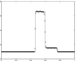
Figure 5.5: Example 5.1: the densities $\rho$ at $t=0.4$. The symbol $\circ$ denotes numerical solution with $200$ cells, while the solid line is exact solution. Left: $P^{K}$-based Runge-Kutta CDG methods; right: $P^{K}$-based RKDG methods. From top to bottom: $K=1,~{}2,~{}3$.

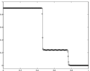
Figure 5.6: Same as Fig.  5.5 except for the velocity $v_{1}$.

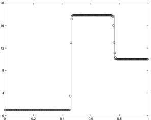
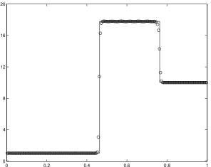
Figure 5.7: Same as Fig.  5.5 except for the pressure $p$.

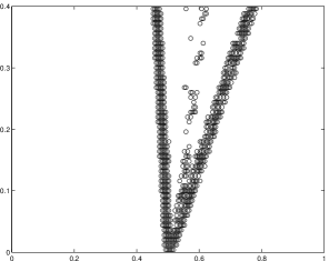
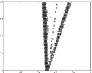
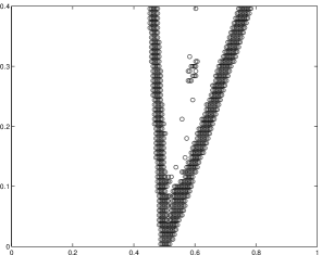
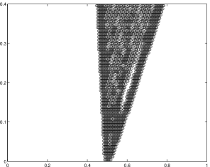
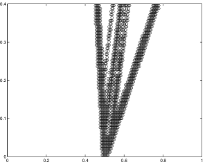
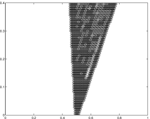
Figure 5.8: Same as Fig. 5.5 except for the “troubled” cells in the $(x,t)$ plane.

Example 5.2 (Riemann problem 2)

The initial data of second Riemann problem is

$$(\rho,v_{1},p)(x,0)=\begin{cases}(10,0.0,1000),&x<0.5,\\ (1,0.0,0.01),&x>0.5,\end{cases}$$

and $\Gamma=5/3$. The solution of this problem will contain a left-moving rarefaction wave, a contact discontinuity, and a right-moving shock wave as $t>0$. The speed of the contact is almost identical to the shock wave so that it is much more challenging for the numerical methods than the first Riemann problem.

The Runge-Kutta CDG methods with new and old calculations of the flux integral over the cell are considered here. The maximum CFL numbers are taken as those in Table 4.3. Figs. 5.9 and 5.10 display the solutions at $t=0.4$ obtained by new and old Runge-Kutta CDG methods with $200$ cells. The density obtained by the old Runge-Kutta CDG methods is slightly better than the new. The CPU times for them with $800$ cells are estimated in Table 5.6. The data show that the new $P^{3}$-based CDG method is faster than the old, there is no obvious difference between two $P^{1}$-based CDG method, but the new $P^{2}$-based CDG method is slower than the old due to a relatively harsh stability condition for the new $P^{2}$-based CDG method.

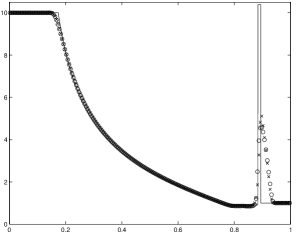
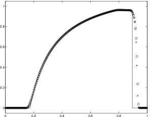
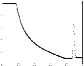
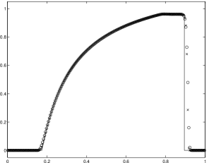
Figure 5.9: Example 5.2: The densities $\rho$ (left) and velocities $v_{1}$ (right) at $t=0.4$. The solid line denotes the exact solution, while the symbol “$\circ$” and “$\times$” are the solutions obtained by using the new and old Runge-Kutta CDG methods with $200$ uniform cells. From top to bottom: $K=1,~{}2,~{}3$.

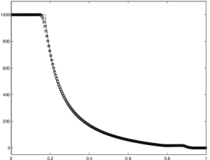
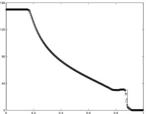
Figure 5.10: Same as Fig. 5.9 except for the pressure $p$ (left) and specific internal energy $e$ (right).

Table 5.6: Example 5.2: CPU times (second) of new and old Runge-Kutta CDG methods with 800 cells.

	new method	old method
$P^{1}$	15.7	15.3
$P^{2}$	55.3	38.4
$P^{3}$	74.2	81.7

5.2 2D case

This section solves some 2D RHD problems by using Runge-Kutta CDG methods on the uniform rectangular meshes. Those problems are the two-dimensional smooth problem, Riemann problems, and shock-bubble interaction problem. The spatial stepsizes in the $x$ and $y$ directions are denoted by $h^{x}$ and $h^{y}$ respectively. Unless otherwise stated, only the third-order accurate TVD Runge-Kutta time discretization (3.8) is employed and and the time step size is taken as

$$\Delta t_{n}=\theta\tau_{n}=\frac{\theta\mu}{\max\limits_{j,k}\Big{(}\frac{\max_{i}|\lambda_{1}^{(i)}(\mbox{\boldmath\small$U$}^{(0)})|}{h^{x}}+\frac{\max_{i}|\lambda_{2}^{(i)}(\mbox{\boldmath\small$U$}^{(0)})|}{h^{y}}\Big{)}},$$ (5.2)

where $\mu$ denotes the CFL number, and “$\max\limits_{j,k}$” denotes the maximum value over the cells $C_{j,k}$ and $D_{j+\frac{1}{2},k+\frac{1}{2}}$, while the values of $\mu$ and $\theta$ will be given in the coming examples.

Example 5.3 (Smooth problem)

This smooth problem has been used in [60] to test the accuracy of numerical methods. The initial data for the primitive variables $V$ is set as

$$\mbox{\boldmath\small$V$}(x,y,0)=\big{(}1+0.2\sin(2\pi(x\cos\alpha+y\sin\alpha)),0.2,0,1\big{)}^{T},$$

where $\alpha=30^{0}$ denotes the angle of the sine wave propagation direction relative to the $x$-axis. The computational domain $\Omega=[0,2/\sqrt{3}]\times[0,2]$ is specified with the periodic boundary conditions, and divided into $N\times 2N$ uniform cells.

Table 5.7  lists the $l^{1}$ errors of density and orders at $t=1$ obtained by using the Runge-Kutta CDG methods, where the fourth-order accurate Runge-Kutta time discretization is employed, $\theta=1$, and the CFL number $\mu$ is taken as $0.3,~{}0.25$, and $0.2$ for $P^{1}$-, $P^{2}$-, and $P^{3}$-based methods, respectively. Those results show that the theoretical order $K+1$ of the $P^{K}$-based Runge-Kutta CDG methods may be achieved.

Table 5.7: Example 5.3: $l^{1}$ errors of the density and orders $t=1$ of the $P^{K}$-based Runge-Kutta CDG methods with $N\times 2N$ cells.

	$N$	without limiter		with limiter in global
		$l^{1}$ error	order	$l^{1}$ error	order
$P^{1}$	10	9.09e-03	–	1.76e-01	–
	20	1.28e-03	2.83	5.28e-02	1.73
	40	3.02e-04	2.08	2.40e-02	1.14
	80	7.56e-05	2.00	6.00e-03	2.00
	160	1.89e-05	2.00	1.46e-03	2.04
	320	4.72e-06	2.00	3.43e-04	2.09
$P^{2}$	10	3.43e-04	–	2.40e-02	–
	20	4.24e-05	3.02	1.33e-03	4.17
	40	5.28e-06	3.01	5.98e-05	4.48
	80	6.59e-07	3.00	4.17e-06	3.84
	160	8.23e-08	3.00	4.20e-07	3.31
	320	1.03e-08	3.00	4.94e-08	3.09
$P^{3}$	10	2.53e-05	–	2.78e-03	–
	20	1.55e-06	4.03	7.26e-05	5.26
	40	9.61e-08	4.01	9.60e-07	6.24
	80	5.99e-09	4.00	1.66e-08	5.85
	160	3.75e-10	4.00	5.07e-10	5.04
	320	2.34e-11	4.00	3.31e-11	3.94

Example 5.4 (Riemann problem 1)

The initial data of the first 2D Riemann problem are

$$(\rho,v_{1},v_{2},p)(x,y,0)=\begin{cases}(0.035145216124503,0,0,0.162931056509027),&x>0,y>0,\\ (0.1,0.7,0,1),&x<0,y>0,\\ (0.5,0,0,1),&x<0,y<0,\\ (0.1,0,0.7,1),&x>0,y<0,\end{cases}$$

where the left and bottom discontinuities are two contact discontinuities and the top and right are two shock waves with the speed of $0.934563275373844$.

In our computations, $\theta$ is taken as 1 or 0.5, and the value of $\mu\theta$ is fixed as $0.3,~{}0.25$, and $0.2$ for the $P^{1}$-, $P^{2}$-, $P^{3}$-based Runge-Kutta CDG methods, respectively. The results at $t=0.8$ obtained by the $P^{K}$-based Runge-Kutta CDG methods are presented in Figs. 5.11, 5.12, and  5.13. Fig. 5.14 gives the density at $t=0.8$ along the line $y=x$. Table 5.8 shows the percentage of “troubled” cells. It is seen that the resolution of $P^{K}$-based RKDG methods is better than $P^{K}$-based Runge-Kutta CDG methods, when $\mu\theta$ is fixed, and the Runge-Kutta CDG methods with small $\theta$ improve the resolution of the discontinuity better than the case of big $\theta$, especially for the $P^{1}$-based CDG method.

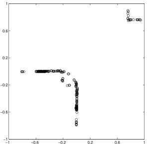
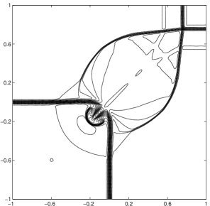
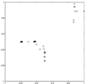
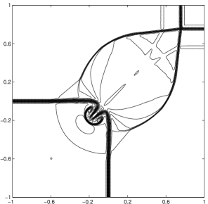
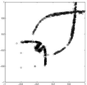
Figure 5.11: Example 5.4: The contour plots of density logarithm $\log\rho$ at (30 equally spaced contour lines from $-1.46$ to $-0.18$) and the “troubled” cells $t=0.8$ obtained with with $300\times 300$ cells. Top: $P^{1}$-based DG, middle: $P^{1}$-based CDG with $\theta=1$, bottom: $P^{1}$-based CDG with $\theta=0.5$.

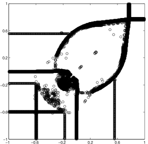
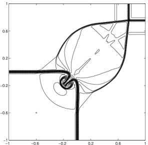
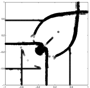
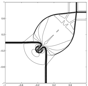
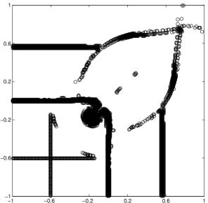
Figure 5.12: Same as Fig. 5.11 except for the $P^{2}$-based Runge-Kutta CDG methods.

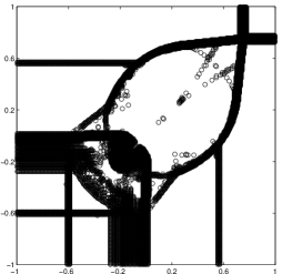
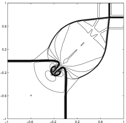
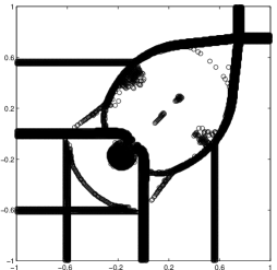
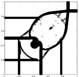
Figure 5.13: Same as Fig. 5.11 except for the $P^{3}$-based Runge-Kutta CDG methods.

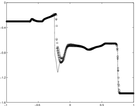
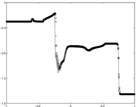
Figure 5.14: Example 5.4: Density logarithm $\log\rho$ at $t=0.8$ along the line $y=x$. The solid line denotes the reference solution obtained by using fifth order accurate WENO scheme with $600\times 600$ uniform cells, while the symbol $\circ$ , $+$ , and “$\square$” are the solutions by the RKDG methods, Runge-Kutta CDG methods ($\theta=0.5$), Runge-Kutta CDG methods ($\theta=1$), respectively. From top to bottom, $K=1,~{}2,~{}3$.

Table 5.8: Example 5.4: The percentage of troubled cells at $t=0.8$.

	non-central DG	CDG
		$\theta=1$	$\theta=0.5$
$P^{1}$	0.19	0.04	1.12
$P^{2}$	5.51	4.78	3.68
$P^{3}$	10.68	8.14	7.95

Table 5.9: Example 5.4: CPU times (second) of the CDG and non-central DG methods.

	CDG	non-central DG
$P^{1}$	5728.7	2491.5
$P^{2}$	16722.4	6119.8
$P^{3}$	54490.8	19287.8

Example 5.5 (Riemann problem 2)

It is about the interaction of four contact discontinuities (vortex sheets) with the same sign (the negative sign) for the ideal relativistic fluid. The initial data may be found in [60]. The new and old Runge-Kutta CDG methods are used to solve this problem. In order to compare the CPU times, the maximum CFL numbers in Table 4.3 and $\theta=1$ are considered for them. Fig. 5.15 displays the contours of density at $t=0.8$. It is seen that the resolutions of the new $P^{1}$- and $P^{2}$-based Runge-Kutta CDG methods are slightly worse than the old, but the difference between two $P^{3}$-based methods are not obvious. Their CPU times listed in Table 5.10 show that for the $P^{2}$ case, the new method is slower than the old, but the new $P^{3}$-based method has a great advantage. It is mainly because the CFL number of the new $P^{2}$-based method is about half of that of the old, while the CFL number of the new $P^{3}$-based method is about two-thirds of the old.

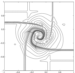
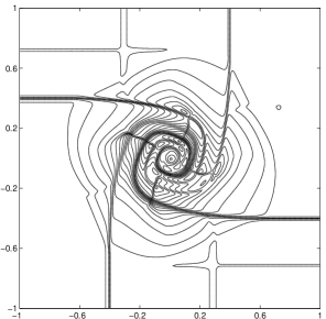
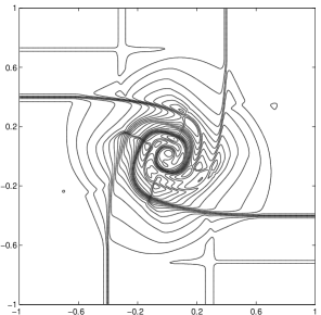
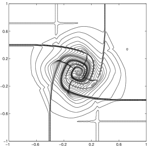
Figure 5.15: Example 5.5: The contour plots of density logarithm $\log\rho$ at $t=0.8$ (30 equally spaced contour lines from $-1.98$ to 0.56) obtained by using $P^{K}$-based Runge-Kutta CDG methods with $300\times 300$ cells. Left: the old, right: the new. From top to bottom, $K=1,~{}2,~{}3$.

Table 5.10: Example 5.5: CPU times (second) of the new and old CDG methods.

	new method	old method
$P^{1}$	2324.5	2460.3
$P^{2}$	14210.2	13611.9
$P^{3}$	30702.3	48538.7

Example 5.6 (Shock and light bubble interaction)

This example describes the interaction between the shock wave and a light bubble, The setup of the problem is as follows. Initially, within the computational domain $[0,325]\times[-45,45]$, there is a left-moving shock wave at $x=265$ with the left and right states

$$(\rho,v_{1},v_{2},p)=\begin{cases}(1,0,0,0.05),&x<265,\\ (1.865225080631180,-0.196781107378299,0,0.15),&x>265.\end{cases}$$

A cylindrical bubble is centered at $(215,0)$ with the radius of 25 in front of the initial shock wave. The fluid within the bubble is in a mechanical equilibrium with the surrounding fluid and lighter than the ambient fluid. The detailed state of the fluid within the bubble is taken as $(\rho,v_{1},v_{2},p)=(0.1358,0,0,0.05)$. In our computations, the domain is divided into $500\times 140$ uniform cells, the CFL numbers $\mu$ for the $P^{1}$-, $P^{2}$-, $P^{3}$-based Runge-Kutta CDG methods are taken as $0.6,0.5,0.4$, respectively, and $\theta=0.5$. Moreover, the parameter $M$ in the modified TVB minmod function is taken as $0.005$, the reflective boundaries are specified at $y=\pm 45$, and the fluid states on two boundaries in $x$-direction are set to the left and right shock wave states, respectively.

Figs. 5.16 and 5.17 show the schlieren images of density and the distributions of “troubled” cells at $t=270$, while Figs. 5.18 and 5.19  give corresponding results at $t=450$. It is seen from those plots that the $P^{K}$-based RKDG methods resolve the complex wave structure better than the $P^{K}$-based Runge-Kutta CDG methods, $P^{3}$-based RKDG methods gives relatively fine wave structure, the distribution of “troubled” cells is very consistent with the solutions, and the “troubled” cell proportions are almost similar for the same order of the two types of DG methods. Table 5.11 gives the percentage of “troubled” cells at two different times. The CPU times are estimated in Table 5.12 and show that the $P^{1}$- and $P^{3}$-based Runge-Kutta CDG methods are faster than corresponding RKDG methods, but the $P^{2}$-based method is an exception.

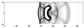
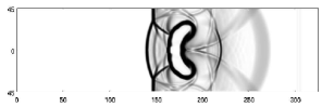
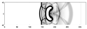
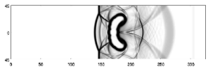
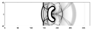
Figure 5.16: Example 5.6: The schlieren images of density at $t=270$ with $500\times 140$ cells. Left: $P^{K}$-based Runge-Kutta CDG methods; right: $P^{K}$-based RKDG methods. From top to bottom, $K=1,2,3$.

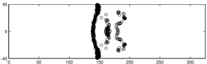
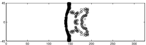
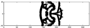
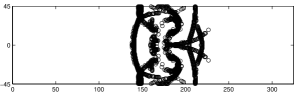
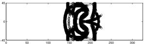
Figure 5.17: Same as Fig. 5.16 except for the “troubled” cells at $t=270$.

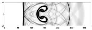
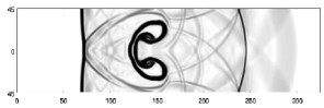
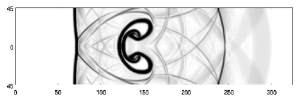
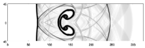
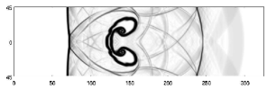
Figure 5.18: Same as Fig. 5.16 except for the schlieren image of density at $t=450$.

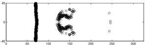
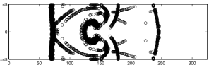
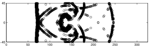
Figure 5.19: Same as Fig. 5.16 except for the “troubled” cells at $t=450$.

Table 5.11: Example 5.6: The percentage of “troubled” cells at two different times.

	$t=270$		$t=450$
	CDG	non-central DG	CDG	non-central DG
$P^{1}$	0.68	0.22	0.71	0.33
$P^{2}$	3.12	3.58	3.40	3.56
$P^{3}$	5.61	5.94	7.11	7.39

Table 5.12: Example 5.6: CPU times (second) of the CDG and non-central DG methods.

	CDG	non-central DG
$P^{1}$	1.93e4	4.03e3
$P^{2}$	6.17e4	1.14e4
$P^{3}$	1.73e5	3.47e4

6 Conclusions

It is much more difficult to solve the relativistic hydrodynamical (RHD) equations than the non-relativistic case. The appearance of Lorentz factor enhances the nonlinearity of the RHD equations, the fluxes can not be formulated in an explicit form of the conservative vector, and there are some inherent physical constraints on the physical state. In practical computations of the RHD system, the primitive variable vector has to be first recovered from the known conservative vector by iteratively solving a nonlinear pressure equation and then the fluxes are evaluated at each time step.

The paper developed the $P^{K}$-based Runge-Kutta CDG methods for the one- and two- dimensional special RHD equations, $K=1,2,3$. In comparison to RKDG methods, the Runge-Kutta CDG methods found two approximate solutions defined on mutually dual meshes. For each mesh, the CDG approximate solutions on its dual mesh were used to calculate the flux values in the cell and on the cell boundary so that the approximate solutions on two mutually dual meshes were coupled with each other, and the use of numerical flux might be avoided. In addition, the Runge-Kutta CDG methods allowed the use of a larger CFL number.

The WENO limiter was adaptively implemented via two steps: the “troubled” cells were first identified by using a modified TVB minmod function, and then the WENO technique is used to locally reconstruct new polynomials of degree $(2K+1)$ replacing the CDG solutions inside the “troubled” cells by using the cell average values of the CDG solutions in the neighboring cells as well as the original cell averages of the “troubled” cells.

The accuracy of the CDG without the numerical dissipation was analyzed and calculation of the flux integrals over the cells was also discussed. Because the DG approximate solutions were discontinuous at the cell interface in general, the integrals over each cell of the DG approximate solutions defined on corresponding dual meshes became a sum of several integrals over subcell of the DG polynomial solutions on corresponding dual meshes, which would lead to that more numerical integration points are needed to ensure the accuracy of Runge-Kutta CDG methods. An attempt was made that only approximate solution on the dual mesh was used to evaluate the flux on the cell boundary for the DG approximations of RHD system on the mesh, thus the integrals of DG solutions over the dual cell might be avoided and the cost of numerical integration was hopefully reduced. For the linear scalar equation, the Fourier method and numerical experiments were used to analyze the stability of such new method, and estimate the CFL numbers for the stability.

Several numerical experiments demonstrated the accuracy, robustness, and discontinuity resolution of our methods. The results showed that the Runge-Kutta CDG methods with WENO limiter were robust and could capture the contact discontinuities, shock waves, and other complex wave structures well, the WENO limiter was only implemented in a few “troubled” cells, the Runge-Kutta CDG methods had obvious advantages in simulating the propagation of slow shock wave in comparison to the RKDG methods. Moreover, the new two-dimensional $P^{3}$-based Runge-Kutta CDG methods could more significantly improve the computational efficiency than the old. In solving RHD problems with large Lorentz factor, or strong discontinuities, or low rest-mass density or pressure etc., it is still possible for the $P^{K}$-based Runge-Kutta CDG methods to give nonphysical solutions. To cure such difficulty, the $P^{0}$-based method may be locally used to replace the $P^{K}$-based. The genuinely effective way is to employ the physical-constraints preserving methods, see e.g. [48, 50].

References

- [1] D.S. Balsara. Riemann solver for relativistic hydrodynamics. J. Comput. Phys., 114:284-297, 1994.
- [2] F. Bassi and S. Rebay. A high-order accurate discontinuous finite element method for the numerical solution of the compressible Navier-Stokes equations. J. Comput. Phys., 131:267-279, 1997.
- [3] R. Biswas, K.D. Devine, and J.E. Flaherty. Parallel, adaptive finite element methods for conservation laws. Appl. Numer. Math., 14:255-283, 1994.
- [4] B. Cockburn, S.C. Hu, and C.-W. Shu. The Runge-Kutta local projection discontinuous Galerkin finite element method for conservation laws IV: the multidimensional case. Math. Comp., 54:545-581, 1990.
- [5] B. Cockburn, F.Y. Li, and C.-W. Shu. Locally divergence-free discontinuous Galerkin methods for the Maxwell equations. J. Comput. Phys., 194:588-610, 2004.
- [6] B. Cockburn, S.Y. Lin, and C.-W. Shu. TVB Runge-Kutta local projection discontinuous Galerkin finite element method for conservation laws III: one-dimensional systems. J. Comput. Phys., 84:90-113, 1989.
- [7] B. Cockburn and C.-W. Shu. TVB Runge-Kutta local projection discontinuous Galerkin finite element method for conservation laws II: general framework. Math. Comp., 52:411-435, 1989.
- [8] B. Cockburn and C.-W. Shu. The Runge-Kutta local projection -discontinuous-Galerkin finite element method for scalar conservation laws. RAIRO Modél. Math. Anal. Numér., 25:337-361, 1991.
- [9] B. Cockburn and C.-W. Shu. The local discontinuous Galerkin method for time-dependent convection-diffusion systems. SIAM J. Numer. Anal., 35:2440-2463, 1998.
- [10] B. Cockburn and C.-W. Shu. The Runge-Kutta discontinuous Galerkin method for conservation laws V: multidimensional systems. J. Comput. Phys., 141:199-224, 1998.
- [11] B. Cockburn and C.-W. Shu. Runge-Kutta discontinuous Galerkin methods for convection-dominated problems. J. Sci. Comput., 16:173-261, 2001.
- [12] W.L. Dai and P.R. Woodward. An iterative Riemann solver for relativistic hydrodynamics. SIAM J. Sci. Comput., 18:982-995, 1997.
- [13] A. Dolezal and S.S.M. Wong. Relativistic hydrodynamics and essentially non-oscillatory shock capturing schemes. J. Comput. Phys., 120:266-277, 1995.
- [14] R. Donat, J.A. Font, J.M. Ibáñez, and A. Marquina. A flux-split algorithm applied to relativistic flows. J. Comput. Phys., 146:58-81, 1998.
- [15] G.C. Duncan and P.A. Hughes. Simulations of relativistic extragalactic jets. Astrophys. J., 436:L119-L122, 1994.
- [16] F. Eulderink and G. Mellema. General relativistic hydrodynamics with a Roe solver. Astrophys. J. Suppl. S., 110:587-623, 1995.
- [17] S.A.E.G. Falle and S.S. Komissarov. An upwind numerical scheme for relativistic hydrodynamics with a general equation of state. Mon. Not. R. Astron. Soc., 278:586-602, 1996.
- [18] P. He and H.Z. Tang. An adaptive moving mesh method for two-dimensional relativistic hydrodynamics. Commun. Comput. Phys., 11:114-146, 2012.
- [19] C.Q. Hu and C.-W. Shu. A discontinuous Galerkin finite element method for Hamilton-Jacobi equations. SIAM J. Sci. Comput., 21:666-690, 1999.
- [20] L. Krivodonova. Limiters for high-order discontinuous Galerkin methods. J. Comput. Phys., 226:879-896, 2007.
- [21] M. Kunik, S. Qamar, and G. Warnecke. Kinetic schemes for the relativistic gas dynamics. Numer. Math., 97:159-191, 2004.
- [22] L.D. Landau and E.M. Lifshitz. Fluid Mechanics. Pergaman Press, 2nd edition, 1987.
- [23] O. Lepsky, C.Q. Hu, and C.-W. Shu. Analysis of the discontinuous Galerkin method for Hamilton-Jacobi equations. Appl. Numer. Math., 33:423-434, 2000.
- [24] F.Y. Li and L.W. Xu. Arbitrary order exactly divergence-free central discontinuous Galerkin methods for ideal MHD equations. J. Comput. Phys., 231:2655-2675, 2012.
- [25] F.Y. Li, L.W. Xu, and S. Yakovlev. Central discontinuous Galerkin methods for ideal MHD equations with the exactly divergence-free magnetic field. J. Comput. Phys., 230:4828-4847, 2011.
- [26] F.Y. Li and S. Yakovlev. A central discontinuous Galerkin method for Hamilton-Jacobi equations. J. Sci. Comput., 45:404-428, 2010.
- [27] Y.J. Liu. Central schemes on overlapping cells. J. Comput. Phys., 209:82-104, 2005.
- [28] Y.J. Liu, C.-W. Shu, E. Tadmor, and M.P. Zhang. Central discontinuous Galerkin methods on overlapping cells with a nonoscillatory hierarchical reconstruction. SIAM J. Numer. Anal., 45:2442-2467, 2007.
- [29] Y.J. Liu, C.-W. Shu, E. Tadmor, and M.P. Zhang. stability analysis of the central discontinuous Galerkin method and a comparison between the central and regular discontinuous Galerkin methods. ESAIM Math. Model. Numer. Anal., 42:593-607, 2008.
- [30] J.M. Martí and E. Müller. Numerical hydrodynamics in special relativity. Living Rev. Relativity, 6:1-100, 2003.
- [31] M.M. May and R.H.White. Hydrodynamic calculations of general-relativistic collapse, Phys. Rev., 141:1232-1241, 1966.
- [32] M.M. May and R.H. White. Stellar dynamics and gravitational collapse, in Methods in Computational Physics, Vol. 7, Astrophysics (B. Alder, S. Fernbach, and M. Rotenberg eds.), Academic Press, 219-258, 1967.
- [33] A. Mignone and G. Bodo. An HLLC Riemann solver for relativistic flows I. hydrodynamics. Mon. Not. R. Astron. Soc., 364:126-136, 2005.
- [34] A. Mignone, T. Plewa, and G. Bodo. The piecewise parabolic method for multidimensional relativistic fluid dynamics. Astrophys. J. Suppl. S., 160:199-219, 2005.
- [35] T. Qin, C.-W. Shu and Y. Yang. Bound-preserving discontinuous Galerkin methods for relativistic hydrodynamics, J. Comput. Phys., 315:323-347, 2016.
- [36] J.X. Qiu and C.-W. Shu. Runge-Kutta discontinuous Galerkin method using WENO limiters. SIAM J. Sci. Comput., 26:907-929, 2005.
- [37] W.H. Reed and T.R. Hill. Triangular mesh methods for neutron transport equation. Technical Report LA-UR-73-479, Los Alamos Scientific Laboratory, 1973.
- [38] J.-F. Remacle, J.E. Flaherty, and M.S. Shephard. An adaptive discontinuous Galerkin technique with an orthogonal basis applied to compressible flow problems. SIAM Rev., 45:53-72, 2003.
- [39] V. Schneider, U. Katscher, D.H. Rischke, B. Waldhauser, J.A. Maruhn, and C.D. Munz. New algorithms for ultra-relativistic numerical hydrodynamics. J. Comput. Phys., 105:92-107, 1993.
- [40] S.H. Shao and H.Z. Tang. Higher-order accurate Runge-Kutta discontinuous Galerkin methods for a nonlinear Dirac model. Discrete Contin. Dyn. Syst. Ser. B, 6:623-640, 2006.
- [41] C.-W. Shu, High order weighted essentially nonoscillatory schemes for convection dominated problems, SIAM Rev., 51(2009), 82-126.
- [42] C.-W. Shu and S. Osher. Efficient implementation of essentially non-oscillatory shock-capturing schemes. J. Comput. Phys., 77:439-471, 1988.
- [43] H.Z. Tang and G. Warnecke. A Runge-Kutta discontinuous Galerkin method for the Euler equations. Computers & Fluids, 34:375-398, 2005.
- [44] D. E. A. van Odyck. Review of numerical special relativistic hydrodynamics. Int. J. Numer. Meth. Fluids, 44:861-884, 2004.
- [45] J.R. Wilson. Numerical study of fluid flow in a Kerr space. Astrophys. J., 173:431-438, 1972.
- [46] K.L. Wu and H.Z. Tang. Finite volume local evolution Galerkin method for two-dimensional relativistic hydrodynamics. J. Comput. Phys., 256:277-307, 2014.
- [47] K.L. Wu and H.Z. Tang. A direct Eulerian GRP scheme for spherically symmetric general relativistic hydrodynamics, SIAM J. Sci. Comput., 38:B458-B489, 2016.
- [48] K.L. Wu and H.Z. Tang. High-order accurate physical-constraints-preserving finite difference WENO schemes for special relativistic hydrodynamics, J. Comput. Phys., 298:539-564, 2015.
- [49] K.L. Wu and H.Z. Tang. Admissible states and physical constraints preserving numerical schemes for special relativistic magnetohydrodynamics, arXiv:1603.06660, 2016.
- [50] K.L. Wu and H.Z.Tang. Physical-constraints-preserving central discontinuous Galerkin methods for special relativistic hydrodynamics with a general equation of state,arXiv: 1607.08332, 2016.
- [51] K.L. Wu, Z.C. Yang, and H.Z. Tang. A third-order accurate direct Eulerian GRP scheme for one-dimensional relativistic hydrodynamics. East Asian J. Appl. Math., 4:95-131, 2014.
- [52] K.L. Wu, Z.C. Yang, and H.Z. Tang. A third-order accurate direct Eulerian GRP scheme for the Euler equations in gas dynamics. J. Comput. Phys., 264:177-208, 2014.
- [53] J.Y. Yang, M.H. Chen, I.N. Tsai, and J.W. Chang. A kinetic beam scheme for relativistic gas dynamics. J. Comput. Phys., 136:19-40, 1997.
- [54] Z.C. Yang, P. He, and H.Z. Tang. A direct Eulerian GRP scheme for relativistic hydrodynamics: one-dimensional case. J. Comput. Phys., 230:7964-7987, 2011.
- [55] Z.C. Yang and H.Z. Tang. A direct Eulerian GRP scheme for relativistic hydrodynamics: two-dimensional case. J. Comput. Phys., 231:2116-2139, 2012.
- [56] L. Del Zanna and N. Bucciantini. An efficient shock-capturing central-type scheme for multidimensional relativistic flows I: Hydrodynamics. Astron. Astrophys., 390:1177-1186, 2002.
- [57] M.P. Zhang and C.-W. Shu. An analysis of three different formulations of the discontinuous Galerkin method for diffusion equations. Math. Models Meth. Appl. Sci., 13:395-413, 2003.
- [58] M.P. Zhang and C.-W. Shu. An analysis of and a comparison between the discontinuous Galerkin and the spectral finite volume methods. Computers & Fluids, 34:581-592, 2005.
- [59] J. Zhao, P. He, and H.Z. Tang. Steger-Warming flux vector splitting method for special relativistic hydrodynamics. Math. Meth. Appl. Sci., 37:1003-1018, 2014.
- [60] J. Zhao and H.Z. Tang. Runge-Kutta discontinuous Galerkin methods with WENO limiter for the special relativistic hydrodynamics. J. Comput. Phys., 24:138-168, 2013.
- [61] J. Zhu and J.X. Qiu. Runge-Kutta discontinuous Galerkin method using WENO-type limiters: three-dimensional unstructured meshes. Commun. Comput. Phys., 11:985-1005, 2012.
- [62] J. Zhu, J.X. Qiu, C.-W. Shu, and M. Dumbser. Runge-Kutta discontinuous Galerkin method using WENO limiters II: unstructured meshes. J. Comput. Phys., 227:4330-4353, 2008.