Krigings Over Space and Time Based on Latent
Low-Dimensional Structures

Abstract

We propose a new approach to represent nonparametrically the linear dependence structure of a spatio-temporal process in terms of latent common factors. Though it is formally similar to the existing reduced rank approximation methods (Section 7.1.3 of Cressie and Wikle, 2011), the fundamental difference is that the low-dimensional structure is completely unknown in our setting, which is learned from the data collected irregularly over space but regularly over time. Furthermore a graph Laplacian is incorporated in the learning in order to take the advantage of the continuity over space, and a new aggregation method via randomly partitioning space is introduced to improve the efficiency. We do not impose any stationarity conditions over space either, as the learning is facilitated by the stationarity in time. Krigings over space and time are carried out based on the learned low-dimensional structure, which is scalable to the cases when the data are taken over a large number of locations and/or over a long time period. Asymptotic properties of the proposed methods are established. Illustration with both simulated and real data sets is also reported.

Key Words: Aggregation via random partitioning; Common factors; Eigenanalysis; Graph Laplacian; Nugget effect; Spatio-temporal processes.

1 Introduction

Kriging, referring to the spatial best linear prediction, is named by Matheron after South African mining engineer Daniel Krige. The key step in kriging is to identify and to estimate the covariance structure. The early applications of kriging are typically based on some parametric models for spatial covariance functions. See Section 4.1 of Cressie and Wikle (2011) and references within. However fitting those parametric covariance models to large spatial or spatio-temporal datasets is conceptually indefensible (Hall, Fisher and Hoffmann, 1994). It also poses serious computational challenges. For example, a spatial kriging with observations from $p$ locations involves inverting a $p\times p$ covariance matrix, which typically requires $O(p^{3})$ operations with $O(p^{2})$ memory. One attractive approach to overcome the computational burden is to introduce reduced rank approximations for the underlying processes. Methods in this category include Higdon (2002) using kernel convolutions, Wikle and Cressie (1999), Kammann and Wand (2003) and Cressie and Johannesson (2008) using low rank basis functions (see also Section 7.1.3 of Cressie and Wikle, 2011), Banerjee et al. (2008) and Finley et al. (2009) using predictive processes, and Tzeng and Huang (2018) using thin-plate splines. However as pointed out by Stein (2008), the reduced rank approximations often fail to capture small-scale correlation structure accurately. An alternative approach is to seek sparse approximations for covariance functions, see, e.g., Gneiting (2002) using compactly supported covariance functions, and Kaufman, Schervish and Nychka (2008) proposing a tempering method by setting the covariances to 0 between any two locations with the distances beyond a threshold. Obviously these approaches miss the correlations among the locations which are distantly apart from each other. Combining together both the ideas of reducing rank and the tempering, Sang and Huang (2012) and Zhang, Sang and Huang (2015) proposed a so-called full scale approximation method for large spatial and spatio-temporal datasets.

In this paper we propose a new nonparametric approach to represent the linear dependence structure of a spatio-temporal process. Different from all the methods stated above, we impose neither any distributional assumptions on the underlying process nor any parametric forms on its covariance function. Under the setting that the observations are taken irregularly over space but regularly in time, we recover the linear dependent structure based on a latent factor representation. No stationarity conditions are imposed over space, though the stationary in time is assumed. Formally our latent factor model is a reduced rank representation. However both the factor process and the factor loadings are completely unknown. This is a marked difference from the aforementioned reduced rank approximation methods. The motivation for our approach is to learn the linear dynamic structure across both space and time directly from data with little subjective assumptions. It captures the dependence across the locations over all distances automatically.

The latent factors and the corresponding loadings are estimated via an eigenanalysis. However it differs from the eigenanalysis for estimating latent factors for multiple time series (cf. Lam and Yao, 2012, and the references within) in at least three aspects. First, we extract the information from the dependence across different locations instead of over time: the whole observations are divided into two sets according to their locations, the estimation boils down to the singular value decomposition (SVD) of the spatial covariance matrix of two data sets. One advantage of this approach is that it is free from the impact of the ‘nugget effect’ in the sense that we do not need to estimate the variances of, for example, measurement errors in order to recover the latent dependence structure. Secondly, we propose new aggregation via randomly partitioning the observations over space to improves the original estimation. This also overcomes the arbitrariness in dividing data in the eigenanalysis. The aggregation proposed is in the spirit of the Bagging of Breiman (1996), though random partitioning instead of bootstraping is used in our approach. Thirdly, we incorporate a graph Laplician (Hastie et al. , 2009, pp.545) into the eigenanalysis to take the advantage of the continuity over space, leading to further improvement in both estimation and kriging.

The number of latent factors is typically small or at least much smaller than the number of locations on which the data are recorded. Consequently the krigings can be performed via only inverting matrices of the size equal to the number of factors. This is particularly appealing when dealing with large datasets. However the SVD for estimating the latent factor structure requires $O(p^{3})$ operation. Nevertheless the nonparametric nature makes our approach easily scalable to large datasets. See Section 3.3 below.

It is worth pointing out that our approach is designed for analyzing spatio-temporal data or pure spatial data but with repeated observations. With the advancement of information technology, large amount of data are collected routinely over space and time nowadays. The surge of the development of statistical methods and theory for modelling and forecasting spatio-temporal processes includes, among others, Smith, Kolenikov and Cox (2003), Jun and Stein (2007), Li, Genton and Sherman (2007), Katzfuss and Cressie (2011), Castruccio and Stein (2013), Guinness and Stein (2013), Zhu, Fan and Kong (2014), Zhang, Sang and Huang (2015), and Wang and Huang (2017). See also the monograph Cressie and Wilkle (2011). In addition to the methods based on low-dimensional covariance structures, the dynamic approach which, typically, specifies the standard Gaussian autoregressive model of order 1 (i.e. AR(1)), coupled with MCMC computation has gained popularity in modelling large spatio-temporal data. Cressie, Shi and Kang (2010) assumed a Gaussian AR(1) model for a low-dimensional latent process and developed a full scale Kalman filter in the context of spatio-temporal modelling. See also Chapter 7 of Cressie and Wilkle (2011).

The rest of the paper is organized as follows. We specify the latent factor structure for a spatio-temporal process in Section 2. The newly proposed estimation methods are spelt out in Section 3. The kriging over space and time is presented in Section 4, in which we also state how to handle missing values. The asymptotic results for the proposed estimation and kriging methods are developed in Section 5. Illustration with both simulated and real data is reported in Section 6. Technical proofs are relegated to the Appendix in a supplementary file.

2 Models

2.1 Setting

Consider spatio-temporal process

$$y_{t}({\mathbf{s}})={\mathbf{z}}_{t}({\mathbf{s}})^{\prime}\boldsymbol{\beta}({\mathbf{s}})+\xi_{t}({\mathbf{s}})+{\varepsilon}_{t}({\mathbf{s}}),\quad t=0,\pm 1,\pm 2,\cdots,\;{\mathbf{s}}\in{\mathcal{S}}\subset\mathcal{R}^{2},$$ (2.1)

where ${\mathbf{z}}_{t}({\mathbf{s}})$ is an $m\times 1$ observable covariant vector, $\boldsymbol{\beta}({\mathbf{s}})$ is a unknown parameter vector, ${\varepsilon}_{t}({\mathbf{s}})$ is unobservable and represents the so-called nugget effect (in space) in the sense that

$$E\{{\varepsilon}_{t}({\mathbf{s}})\}=0,\quad\mbox{Var}\{{\varepsilon}_{t}({\mathbf{s}})\}=\sigma({\mathbf{s}})^{2},\quad{\rm Cov}\{{\varepsilon}_{t_{1}}({\mathbf{u}}),{\varepsilon}_{t_{2}}({\mathbf{v}})\}=0\;\;\forall\;(t_{1},{\mathbf{u}})\neq(t_{2},{\mathbf{v}}),$$ (2.2)

$\xi_{t}({\mathbf{s}})$ is a latent spatio-temporal process satisfying the conditions

$$E\{\xi_{t}({\mathbf{s}})\}=0,\qquad{\rm Cov}\{\xi_{t_{1}}({\mathbf{u}}),\xi_{t_{2}}({\mathbf{v}})\}=\Sigma_{|t_{1}-t_{2}|}({\mathbf{u}},{\mathbf{v}}).$$ (2.3)

Consequently, $y_{t}({\mathbf{s}})-{\mathbf{z}}_{t}({\mathbf{s}})^{\prime}\boldsymbol{\beta}({\mathbf{s}})$ is (weakly) stationary in time $t$, $E\{y_{t}({\mathbf{s}})-{\mathbf{z}}_{t}({\mathbf{s}})^{\prime}\boldsymbol{\beta}({\mathbf{s}})\}=0$, and

$${\rm Cov}\{y_{t_{1}}({\mathbf{u}})-{\mathbf{z}}_{t_{1}}({\mathbf{u}})^{\prime}\boldsymbol{\beta}({\mathbf{u}}),\;y_{t_{2}}({\mathbf{v}})-{\mathbf{z}}_{t_{2}}({\mathbf{v}})^{\prime}\boldsymbol{\beta}({\mathbf{v}})\}=\Sigma_{|t_{1}-t_{2}|}({\mathbf{u}},{\mathbf{v}})+\sigma({\mathbf{u}})^{2}I\{(t_{1},{\mathbf{u}})=(t_{2},{\mathbf{v}})\}.$$ (2.4)

Furthermore we assume that $\Sigma_{t}({\mathbf{u}},{\mathbf{v}})$ is continuous in ${\mathbf{u}}$ and ${\mathbf{v}}$.

Model (2.1) does not impose any stationarity conditions over space. However it requires that $y_{t}(\cdot)-{\mathbf{z}}_{t}(\cdot)^{\prime}\boldsymbol{\beta}(\cdot)$ is second order stationary in time $t$, which enables the learning of the dependence across different locations and times. In practice the data often show some trends and seasonal patterns in time. The existing detrend and deseasonality methods in time series analysis can be applied to make data stationary in time.

2.2 A finite dimensional representation for $\xi_{t}({\mathbf{s}})$

Let $L_{2}({\mathcal{S}})$ be the Hilbert space consisting of all the square integrable functions defined on ${\mathcal{S}}$ equipped with the inner product

$$\mbox{$\langle f,g\rangle$}=\int_{{\mathcal{S}}}f({\mathbf{s}})g({\mathbf{s}})d{\mathbf{s}},\qquad f,g\in L_{2}({\mathcal{S}}).$$ (2.5)

We assume that the latent process $\xi_{t}({\mathbf{s}})$ admits a finite-dimensional structure:

$$\xi_{t}({\mathbf{s}})=\sum_{j=1}^{d}a_{j}({\mathbf{s}})x_{tj},$$ (2.6)

where $a_{1}(\cdot),\cdots,a_{d}(\cdot)$ are deterministic and linear independent functions (i.e. none of them can be written as a linear combination of the others) in the Hilbert space $L_{2}({\mathcal{S}})$, and $x_{t1},\cdots,x_{td}$ are $d$ latent time series. Obviously $a_{1}(\cdot),\cdots,a_{d}(\cdot)$ (as well as $x_{t1},\cdots,x_{td}$) are not uniquely defined by (2.6), as they can be replaced by any of their non-degenerate linear transformations. There is no loss of generality in assuming that $a_{1}(\cdot),\cdots,a_{d}(\cdot)$ are orthonormal in the sense that

$$\mbox{$\langle a_{i},a_{j}\rangle$}=I(i=j),$$ (2.7)

as any set of linear independent functions in a Hilbert space can be standardized to this effect. Let ${\mathbf{x}}_{t}=(x_{t1},\cdots,x_{td})^{\prime}$. It follows from (2.3) that ${\mathbf{x}}_{t}$ is a $d$-variant stationary time series with mean $\bf 0$, and

$$\Sigma_{0}({\mathbf{u}},{\mathbf{v}})={\rm Cov}\{\xi_{t}({\mathbf{u}}),\xi_{t}({\mathbf{v}})\}=\sum_{i,j=1}^{d}a_{i}({\mathbf{u}})a_{j}({\mathbf{v}})\sigma_{ij},$$ (2.8)

where $\sigma_{ij}$ is the $(i,j)$-th element of $\mbox{Var}({\mathbf{x}}_{t})$. Let

$$\Sigma_{0}\circ f({\mathbf{s}})=\int_{\mathcal{S}}\Sigma_{0}({\mathbf{s}},{\mathbf{u}})f({\mathbf{u}})d{\mathbf{u}},\qquad f\in L_{2}({\mathcal{S}}).$$ (2.9)

Then $\Sigma_{0}$ is a non-negative definite operator defined on $L_{2}({\mathcal{S}})$. See Appendix A of Bathia et al. (2010) for some basic facts on the operators in Hilbert spaces. It follows from Mercer’s theorem (Mercer 1909) that $\Sigma_{0}$ admits the spectral decomposition

$$\Sigma_{0}({\mathbf{u}},{\mathbf{v}})=\sum_{j=1}^{d}\lambda_{j}\varphi_{j}({\mathbf{u}})\varphi_{j}({\mathbf{v}}),$$ (2.10)

where $\lambda_{1}\geq\cdots\geq\lambda_{d}>0$ are the $d$ positive eigenvalues of $\Sigma_{0}({\mathbf{u}},{\mathbf{v}})$, and $\varphi_{1},\cdots,\varphi_{d}\in L_{2}({\mathcal{S}})$ are the corresponding eigenfunctions, i.e.

$$\Sigma_{0}\circ\varphi_{j}({\mathbf{s}})=\int_{\mathcal{S}}\Sigma_{0}({\mathbf{s}},{\mathbf{u}})\varphi_{j}({\mathbf{u}})d{\mathbf{u}}=\lambda_{j}\varphi_{j}({\mathbf{s}}).$$ (2.11)

See Proposition 1 below.

Proposition 1

Let rank$(\mbox{Var}({\mathbf{x}}_{t}))=d$. Then the following assertions hold.

• $\Sigma_{0}$ defined in (2.9) has exactly $d$ positive eigenvalues.

• The $d$ corresponding orthonormal eigenfunctions can be expressed as

  $$\varphi_{i}({\mathbf{s}})=\sum_{j=1}^{d}\gamma_{ij}a_{j}({\mathbf{s}}),\qquad i=1,\cdots,d,$$

  where $\boldsymbol{\gamma}_{i}\equiv(\gamma_{i1},\cdots,\gamma_{id})^{\prime}$, $i=1,\cdots,d$, are $d$ orthonormal eigenvectors of matrix $\mbox{Var}({\mathbf{x}}_{t})$.

The above proposition shows that the finite-dimensional structure (2.6) can be identified via the covariance functions of $\xi_{t}({\mathbf{s}})$, though the representation of (2.6) itself is not unique. Note that the linear space spanned by the eigenfunctions $\varphi_{1}(\cdot),\cdots,\varphi_{d}(\cdot)$ is called the kernel reproducing Hilbert space (KRHS) by $\Sigma_{0}(\cdot,\,\cdot)$, and $\{a_{j}(\cdot)\}$ and $\{\varphi_{j}(\cdot)\}$ are two orthonormal bases for this KRHS. Furthermore any orthonormal basis of this KRHS can be taken as $a_{1}(\cdot),\cdots,a_{d}(\cdot)$. In Section 3 below, the estimation for $a_{1}(\cdot),\cdots,a_{d}(\cdot)$ will be constructed in this spirit.

3 Estimation

Let $\{(y_{t}({\mathbf{s}}_{i}),{\mathbf{z}}_{t}({\mathbf{s}}_{i})),\;i=1,\cdots,p,\;t=1,\cdots,n\}$ be the available observations over space and time, where ${\mathcal{S}}_{o}\equiv\{{\mathbf{s}}_{1},\cdots,{\mathbf{s}}_{p}\}\subset{\mathcal{S}}$ are typically irregularly spaced. The total number of observations is $n\cdot p$.

3.1 Estimation for finite dimensional representations of $\xi_{t}({\mathbf{s}})$

To simplify the notation, we first consider a special case $\boldsymbol{\beta}({\mathbf{s}})\equiv 0$ in (2.1) in Sections 3.1 & 3.2. Section 3.4 below considers the least squares regression estimation for $\boldsymbol{\beta}({\mathbf{s}})$. Then the procedures describe in Sections 3.1 & 3.2 still apply if $\{y_{t}({\mathbf{s}}_{i})\}$ are replaced by the residuals from the regression estimation.

Now under (2.6),

$$y_{t}({\mathbf{s}})=\xi_{t}({\mathbf{s}})+{\varepsilon}_{t}({\mathbf{s}})=\sum_{j=1}^{d}a_{j}({\mathbf{s}})x_{tj}+{\varepsilon}_{t}({\mathbf{s}}).$$ (3.1)

To exclude nugget effect in our estimation, we divide $p$ locations ${\mathbf{s}}_{1},\cdots,{\mathbf{s}}_{p}$ into two sets ${\mathcal{S}}_{1}$ and ${\mathcal{S}}_{2}$ with, respectively, $p_{1}$ and $p_{2}$ elements, and $p_{1}+p_{2}=p$. Let ${\mathbf{y}}_{t,i}$ be a vector consisting of $y_{t}({\mathbf{s}})$ with ${\mathbf{s}}\in{\mathcal{S}}_{i}$, $i=1,2$. Then ${\mathbf{y}}_{t,1},{\mathbf{y}}_{t,2}$ are two vectors with lengths $p_{1}$ and $p_{2}$ respectively. Denoted by $\boldsymbol{\xi}_{t,1},\,\boldsymbol{\xi}_{t,2}$ the corresponding vectors consisting of $\xi_{t}(\cdot)$. It follows from (3.1) that

$${\mathbf{y}}_{t,1}=\boldsymbol{\xi}_{t,1}+\mbox{\boldmath$\varepsilon$}_{t,1}={\mathbf{A}}_{1}{\mathbf{x}}_{t}+\mbox{\boldmath$\varepsilon$}_{t,1},\qquad{\mathbf{y}}_{t,2}=\boldsymbol{\xi}_{t,2}+\mbox{\boldmath$\varepsilon$}_{t,2}={\mathbf{A}}_{2}{\mathbf{x}}_{t}+\mbox{\boldmath$\varepsilon$}_{t,2},$$ (3.2)

where ${\mathbf{A}}_{i}$ is a $p_{i}\times d$ matrix, its rows consist of the coefficients $a_{j}(\cdot)$ on the RHS of (3.1), and $\mbox{\boldmath$\varepsilon$}_{t,i}$ consists of ${\varepsilon}_{t}({\mathbf{s}})$ with ${\mathbf{s}}\in{\mathcal{S}}_{i}$. There is no loss of generality in assuming ${\mathbf{A}}_{1}^{\prime}{\mathbf{A}}_{1}={\mathbf{I}}_{d}$. This can be achieved by performing an orthogonal-triangular (QR) decomposition ${\mathbf{A}}_{1}=\boldsymbol{\Gamma}{\mathbf{R}}$, and replacing $({\mathbf{A}}_{1},{\mathbf{x}}_{t})$ by $(\boldsymbol{\Gamma},{\mathbf{R}}{\mathbf{x}}_{t})$ in the first equation in (3.2). Note ${\mathcal{M}}({\mathbf{A}}_{1})={\mathcal{M}}(\boldsymbol{\Gamma})$, where ${\mathcal{M}}({\mathbf{A}})$ denotes the linear space spanned by the columns of matrix ${\mathbf{A}}$. Thus ${\mathcal{M}}({\mathbf{A}}_{1})$ does not change from imposing the condition ${\mathbf{A}}_{1}^{\prime}{\mathbf{A}}_{1}={\mathbf{I}}_{d}$. Similar we may also assume ${\mathbf{A}}_{2}^{\prime}{\mathbf{A}}_{2}={\mathbf{I}}_{d}$, which however implies that ${\mathbf{x}}_{t}$ in the second equation in (3.2) is unlikely to be the same as that in the first equation. Hence we may re-write (3.2) as

$${\mathbf{y}}_{t,1}={\mathbf{A}}_{1}{\mathbf{x}}_{t}+\mbox{\boldmath$\varepsilon$}_{t,1},\qquad{\mathbf{y}}_{t,2}={\mathbf{A}}_{2}{\mathbf{x}}_{t}^{\star}+\mbox{\boldmath$\varepsilon$}_{t,2},$$ (3.3)

where ${\mathbf{A}}_{1}^{\prime}{\mathbf{A}}_{1}={\mathbf{A}}_{2}^{\prime}{\mathbf{A}}_{2}={\mathbf{I}}_{d}$, ${\mathbf{x}}_{t}^{\star}={\mathbf{Q}}{\mathbf{x}}_{t}$, and ${\mathbf{Q}}$ is an invertible $d\times d$ matrix. Note that $({\mathbf{A}}_{1},{\mathbf{x}}_{t})$ and $({\mathbf{A}}_{2},{\mathbf{x}}_{t}^{\star})$ are still not uniquely defined in (3.3), as they can be replaced, respectively, by $({\mathbf{A}}_{1}\boldsymbol{\Gamma}_{1},\boldsymbol{\Gamma}_{1}^{\prime}{\mathbf{x}}_{t})$ and $({\mathbf{A}}_{2}\boldsymbol{\Gamma}_{2},\boldsymbol{\Gamma}_{2}^{\prime}{\mathbf{x}}_{t}^{\star})$ for any $d\times d$ orthogonal matrices $\boldsymbol{\Gamma}_{1}$ and $\boldsymbol{\Gamma}_{2}$. However ${\mathcal{M}}({\mathbf{A}}_{1})$ and ${\mathcal{M}}({\mathbf{A}}_{2})$ are uniquely defined by (3.3).

Since ${\mathbf{y}}_{t,1}$ and ${\mathbf{y}}_{t,2}$ have no common elements, it follows from (3.1) and (2.2) that

$$\boldsymbol{\Sigma}\equiv{\rm Cov}({\mathbf{y}}_{t,1},{\mathbf{y}}_{t,2})={\mathbf{A}}_{1}{\rm Cov}({\mathbf{x}}_{t},{\mathbf{x}}_{t}^{\star}){\mathbf{A}}_{2}^{\prime}.$$ (3.4)

Note that ${\rm Cov}({\mathbf{x}}_{t},{\mathbf{x}}_{t}^{\star})=\mbox{Var}({\mathbf{x}}_{t}){\mathbf{Q}}$. When $p\gg d$, it is reasonable to assume that rank$(\boldsymbol{\Sigma})={\rm rank}\{{\rm Cov}({\mathbf{x}}_{t},{\mathbf{x}}_{t}^{\star})\}={\rm rank}\{\mbox{Var}({\mathbf{x}}_{t})\}=d$. Let

$$\boldsymbol{\Sigma}\boldsymbol{\Sigma}^{\prime}={\mathbf{A}}_{1}{\rm Cov}({\mathbf{x}}_{t},{\mathbf{x}}_{t}^{\star}){\rm Cov}({\mathbf{x}}_{t}^{\star},{\mathbf{x}}_{t}){\mathbf{A}}_{1}^{\prime},\qquad\boldsymbol{\Sigma}^{\prime}\boldsymbol{\Sigma}={\mathbf{A}}_{2}{\rm Cov}({\mathbf{x}}_{t}^{\star},{\mathbf{x}}_{t}){\rm Cov}({\mathbf{x}}_{t},{\mathbf{x}}_{t}^{\star}){\mathbf{A}}_{2}^{\prime}.$$ (3.5)

Then these two matrices share the same $d$ positive eigenvalues, and $\boldsymbol{\Sigma}\boldsymbol{\Sigma}^{\prime}{\mathbf{b}}=0$ for any vector ${\mathbf{b}}$ perpendicular to ${\mathcal{M}}({\mathbf{A}}_{1})$. Therefore, the $d$ orthonormal eigenvectors of matrix $\boldsymbol{\Sigma}\boldsymbol{\Sigma}^{\prime}$ corresponding to its $d$ positive eigenvalues can be taken as the columns of ${\mathbf{A}}_{1}$. Similarly the $d$ orthonormal eigenvectors of matrix $\boldsymbol{\Sigma}^{\prime}\boldsymbol{\Sigma}$ corresponding to its $d$ positive eigenvalues can be taken as the columns of ${\mathbf{A}}_{2}$. We construct the estimators for ${\mathbf{A}}_{1},\,{\mathbf{A}}_{2}$ based on this observation.

Let $\widehat{\boldsymbol{\Sigma}}$ be the sample covariance of ${\mathbf{y}}_{t,1}$ and ${\mathbf{y}}_{t,2}$, i.e.

$$\widehat{\boldsymbol{\Sigma}}={1\over n}\sum_{t=1}^{n}({\mathbf{y}}_{t,1}-\bar{\mathbf{y}}_{1})({\mathbf{y}}_{t,2}-\bar{\mathbf{y}}_{2})^{\prime},$$ (3.6)

where $\bar{\mathbf{y}}_{i}=n^{-1}\sum_{t}{\mathbf{y}}_{t,i}$. Let $\widehat{\lambda}_{1}\geq\widehat{\lambda}_{2}\geq\cdots$ be the eigenvalues of $\widehat{\boldsymbol{\Sigma}}\widehat{\boldsymbol{\Sigma}}^{\prime}$. A natural estimator for $d$ is defined as

$$\widehat{d}=\max_{1\leq j<p_{*}}\widehat{\lambda}_{j}\big{/}\widehat{\lambda}_{j+1},$$ (3.7)

where $p_{*}\ll\min(p_{1},\,p_{2})$ is a prespecified integer (e.g. $p_{*}=\min(p_{1},\,p_{2})/2$). This estimation method is based on the fact that $\lambda_{j}/\lambda_{j+1}$ are positive and finite constants for $j=1,\cdots,d-1$, and $\lambda_{d}/\lambda_{d+1}=\infty$. However $\lambda_{j}/\lambda_{j+1}$ is asymptotically ‘$0/0$’ for $j=d+1,\cdots,p-1$. In practice, we mitigate this difficulty by comparing the ratios for $j<p_{*}\ll\min(p_{1},p_{2})$. Asymptotic properties of the ratio estimators under different settings have been established in, e.g. Lam and Yao (2012), Chang et al. (2015), and Zhang et al. (2018). The (fine) finite sample performance of the ratio estimators are also reported in those papers.

Consequently the $\widehat{d}$ orthonormal eigenvectors of $\widehat{\boldsymbol{\Sigma}}\widehat{\boldsymbol{\Sigma}}^{\prime}$ (or $\widehat{\boldsymbol{\Sigma}}^{\prime}\widehat{\boldsymbol{\Sigma}}$), corresponding to the eigenvalues $\widehat{\lambda}_{1},\cdots,\widehat{\lambda}_{\widehat{d}}$, can be taken as the estimated columns of ${\mathbf{A}}_{1}$ (or ${\mathbf{A}}_{2}$). However such an estimator ignores the fact that $\xi_{t}(\cdot)$ is continuous over the set ${\mathcal{S}}$, which should be taken into account to improve the estimation. To achieve this, denoted by ${\mathbf{s}}_{1}^{1},\cdots,{\mathbf{s}}_{p_{1}}^{1}$ the $p_{1}$ locations in ${\mathcal{S}}_{1}$ arranged according to the order such that the $j$-th component of ${\mathbf{y}}_{t,1}$ is the observation taken at the location ${\mathbf{s}}^{1}_{j}$. We define a graph Laplacian ${\mathbf{L}}\equiv{\mathbf{G}}-{\mathbf{W}}$, where ${\mathbf{W}}=(w_{ij})$ is a weight matrix with $w_{ii}=0$ and, e.g. $w_{ij}=1/(1+\|{\mathbf{s}}_{i}^{1}-{\mathbf{s}}_{j}^{1}\|)$ ($\|\cdot\|$ denotes the Euclidean norm) for $i\neq j$, and ${\mathbf{G}}=(g_{ij})$ with $g_{ii}=\sum_{j}w_{ij}$ and $g_{ij}=0$ for all $i\neq j$. Then it holds that for any column vector ${\mathbf{a}}=(a_{1},\cdots,a_{p})^{\prime}$,

$${\mathbf{a}}^{\prime}{\mathbf{L}}{\mathbf{a}}=\sum_{i=1}^{p}g_{ii}a_{i}^{2}-\sum_{i,j=1}^{p}w_{ij}a_{i}a_{j}={1\over 2}\sum_{i,j=1}^{p}w_{ij}(a_{i}-a_{j})^{2}.$$

See, e.g., Hastie, Tibshirani and Friedman (2009, pp.545). By requiring ${\mathbf{a}}^{\prime}{\mathbf{L}}{\mathbf{a}}\leq c_{0}$ for some small positive constant $c_{0}$, the components of ${\mathbf{a}}$ at the nearby locations will be close with each other. Hence the columns of ${\mathbf{A}}_{1}$ are obtained by solving the following optimization problem:

$$\widehat{\boldsymbol{\gamma}}_{1}=\arg\max_{\boldsymbol{\gamma}}\boldsymbol{\gamma}^{\prime}\widehat{\boldsymbol{\Sigma}}\widehat{\boldsymbol{\Sigma}}^{\prime}\boldsymbol{\gamma}\quad{\rm subject\;to}\;\;\|\boldsymbol{\gamma}\|=1\;\;{\rm and}\;\;\boldsymbol{\gamma}^{\prime}{\mathbf{L}}\boldsymbol{\gamma}\leq c_{0},$$

and for $j=2,\cdots,\widehat{d}$,

$$\widehat{\boldsymbol{\gamma}}_{j}=\arg\max_{\boldsymbol{\gamma}}\boldsymbol{\gamma}^{\prime}\widehat{\boldsymbol{\Sigma}}\widehat{\boldsymbol{\Sigma}}^{\prime}\boldsymbol{\gamma}\quad{\rm subject\;to}\;\;\|\boldsymbol{\gamma}\|=1,\;\;\boldsymbol{\gamma}^{\prime}\widehat{\boldsymbol{\gamma}}_{i}=0\;{\rm for\;}1\leq i<j,\;\;{\rm and}\;\;\boldsymbol{\gamma}^{\prime}{\mathbf{L}}\boldsymbol{\gamma}\leq c_{0}.$$

The above constrained optimization problem can be recast as an eigen-problem for the symmetric (but not necessarily non-negative definite) matrix $\widehat{\boldsymbol{\Sigma}}\widehat{\boldsymbol{\Sigma}}^{\prime}-\tau{\mathbf{L}}$ stated below, where $\tau>0$ controls the penalty according to ${\mathbf{L}}$.

Find the orthonormal eigenvectors $\widehat{\boldsymbol{\gamma}}_{1},\cdots,\widehat{\boldsymbol{\gamma}}_{\widehat{d}}$ of $\widehat{\boldsymbol{\Sigma}}\widehat{\boldsymbol{\Sigma}}^{\prime}-\tau{\mathbf{L}}$ corresponding to its $\widehat{d}$ largest eigenvalues.

Denote the resulting estimator for the loading matrix ${\mathbf{A}}_{1}$ by

$$\widehat{\mathbf{A}}_{1}=(\widehat{\boldsymbol{\gamma}}_{1},\cdots,\widehat{\boldsymbol{\gamma}}_{p_{1}}).$$ (3.8)

The estimator for ${\mathbf{A}}_{2}$, denoted by $\widehat{\mathbf{A}}_{2}$, is constructed in the same manner.

By (3.2), the estimators for the two different representations of the latent processes are defined as

$$\widehat{\mathbf{x}}_{t}=\widehat{\mathbf{A}}_{1}^{\prime}{\mathbf{y}}_{t,1},\qquad\widehat{\mathbf{x}}_{t}^{\star}=\widehat{\mathbf{A}}_{2}^{\prime}{\mathbf{y}}_{t,2}.$$ (3.9)

Consequently,

$$\widehat{\boldsymbol{\xi}}_{t,1}=\widehat{\mathbf{A}}_{1}\widehat{\mathbf{x}}_{t}=\widehat{\mathbf{A}}_{1}\widehat{\mathbf{A}}_{1}^{\prime}{\mathbf{y}}_{t,1},\qquad\widehat{\boldsymbol{\xi}}_{t,2}=\widehat{\mathbf{A}}_{2}\widehat{\mathbf{x}}_{t}^{\star}=\widehat{\mathbf{A}}_{2}\widehat{\mathbf{A}}_{2}^{\prime}{\mathbf{y}}_{t,2}.$$ (3.10)

See also (3.2).

Remark 1

(i) The assumption that matrix $\boldsymbol{\Sigma}$ in (3.4) has rank $d$ implies that all the latent factors are spatially correlated; see (3.1). In the unlikely scenarios that some latent factors are only serially correlated but spatially uncorrelated, we should include autocovariance matrices in the estimation (Lam and Yao, 2012). To this end, let

$$\widehat{\boldsymbol{\Sigma}}_{i}(k)={1\over n}\sum_{t=1}^{n-k}({\mathbf{y}}_{t+k,i}-\bar{\mathbf{y}}_{i})({\mathbf{y}}_{t,i}-\bar{\mathbf{y}}_{i})^{\prime},\quad\widehat{\boldsymbol{\Sigma}}_{12}(k)={1\over n}\,\sum_{t=\max\{1,-k\}}^{\min\{n-k,n\}}({\mathbf{y}}_{t+k,1}-\bar{\mathbf{y}}_{1})({\mathbf{y}}_{t,2}-\bar{\mathbf{y}}_{2})^{\prime}.$$

Assume $p_{1}=p_{2}$ for simplicity. Put

$${\mathbf{M}}_{1}=\widehat{\boldsymbol{\Sigma}}\widehat{\boldsymbol{\Sigma}}^{\prime}+\sum_{j=1}^{k_{0}}\big{\{}\widehat{\boldsymbol{\Sigma}}_{1}(j)\widehat{\boldsymbol{\Sigma}}_{1}(j)^{\prime}+\widehat{\boldsymbol{\Sigma}}_{12}(j)\widehat{\boldsymbol{\Sigma}}_{12}(j)^{\prime}+\widehat{\boldsymbol{\Sigma}}_{12}(-j)\widehat{\boldsymbol{\Sigma}}_{12}(-j)^{\prime}\},$$

$${\mathbf{M}}_{2}=\widehat{\boldsymbol{\Sigma}}^{\prime}\widehat{\boldsymbol{\Sigma}}+\sum_{j=1}^{k_{0}}\big{\{}\widehat{\boldsymbol{\Sigma}}_{2}(j)\widehat{\boldsymbol{\Sigma}}_{2}(j)^{\prime}+\widehat{\boldsymbol{\Sigma}}_{12}(j)^{\prime}\widehat{\boldsymbol{\Sigma}}_{12}(j)+\widehat{\boldsymbol{\Sigma}}_{12}(-j)^{\prime}\widehat{\boldsymbol{\Sigma}}_{12}(-j)\},$$

where $\widehat{\boldsymbol{\Sigma}}$ is defined in (3.6), and $k_{0}\geq 1$ is an integer. Then we replace $\widehat{\boldsymbol{\Sigma}}\widehat{\boldsymbol{\Sigma}}^{\prime}$ by ${\mathbf{M}}_{1}$ for computing $\widehat{\mathbf{A}}_{1}$ in (3.8), and replace $\widehat{\boldsymbol{\Sigma}}^{\prime}\widehat{\boldsymbol{\Sigma}}$ by ${\mathbf{M}}_{2}$ for computing $\widehat{\mathbf{A}}_{2}$. Empirical evidences in modelling high-dimensional time series indicate that the estimation is not sensitive to the choice of $k_{0}$, small values of $k_{0}$ such as 1 to 5 are sufficient for most applications (Lam et al. 2011, Lam and Yao 2012, Chang et al. 2015). Since using ${\mathbf{M}}_{1}$ and ${\mathbf{M}}_{2}$ does not add anything fundamentally new, we proceed with the simple version only.

(ii) The proposed procedure encapsulates all the dependence across space and time into $d$ latent factors. Those latent factors, specified objectively by sample covariances (and autocovariances) of the data, capture all the linear correlations parsimoniously. The real data example in Section 6.2 below, and also those not shown in this paper, indicate that the estimated $d$ is often small.

3.2 Aggregating via random partitioning

The estimation for the latent variable $\xi_{t}(\cdot)$ depends on partitioning ${\mathcal{S}}_{o}=\{{\mathbf{s}}_{1},\cdots,{\mathbf{s}}_{p}\}$ into two non-overlapping sets ${\mathcal{S}}_{1}$ and ${\mathcal{S}}_{2}$; see (3.10). Since the estimation procedure presented in Section 3.1 puts ${\mathcal{S}}_{1}$ and ${\mathcal{S}}_{2}$ on equal footing, we set $p_{1}=[p/2]$ and $p_{2}=p-p_{1}$. By randomly dividing ${\mathcal{S}}_{o}$ into ${\mathcal{S}}_{1}$ and ${\mathcal{S}}_{2}$ with the sizes $p_{1}$ and $p_{2}$ respectively, the estimates for $\boldsymbol{\xi}_{t,1}$ and $\boldsymbol{\xi}_{t,2}$ are obtained as in (3.10). We repeat this randomization $J$ times, where $J\geq 1$ is a large integer, leading to the $J$ pairs of the estimates $(\widehat{\boldsymbol{\xi}}_{t,1}^{j},\,\widehat{\boldsymbol{\xi}}_{t,2}^{j})$ for $j=1,\cdots,J.$ The aggregating estimator over the randomized partitions is

$$\widetilde{\xi}_{t}({\mathbf{s}}_{i})={1\over J}\sum_{j=1}^{J}\widehat{\xi}_{t}^{j}({\mathbf{s}}_{i}),\qquad j=1,\cdots,p,$$ (3.11)

where $\widehat{\xi}_{t}^{j}({\mathbf{s}}_{i})$ is a component of either $\widehat{\boldsymbol{\xi}}_{t,1}^{j}$ or $\widehat{\boldsymbol{\xi}}_{t,2}^{j}$, depending on ${\mathbf{s}}_{i}\in{\mathcal{S}}_{1}$ or ${\mathcal{S}}_{2}$ in the $j$-th randomized partition of ${\mathcal{S}}_{o}$. Similar to the Bagging method of Breiman (1996), the choice of $J$ is not critical. In our numerical experiments, we set $J=100$.

Theorem 1

For $k=1,\cdots,n$ and $\ell=1,\cdots,p$,

$$E\Big{(}\big{\{}\widetilde{\xi}_{k}({\mathbf{s}}_{\ell})-y_{k}({\mathbf{s}}_{\ell})\big{\}}^{2}\Big{|}\{y_{t}({\mathbf{s}}_{i})\}\Big{)}\leq E\Big{(}\big{\{}\widehat{\xi}_{k}({\mathbf{s}}_{\ell})-y_{k}({\mathbf{s}}_{\ell})\big{\}}^{2}\Big{|}\{y_{t}({\mathbf{s}}_{i})\}\Big{)},$$ (3.12)

and

$$\mathrm{E}\Big{(}{1\over np}\sum_{t=1}^{n}\sum_{j=1}^{p}\big{\{}\widetilde{\xi}_{t}({\mathbf{s}}_{j})-\xi_{t}({\mathbf{s}}_{j})\}^{2}\Big{|}\{\xi_{t}({\mathbf{s}}_{i}),\,y_{t}({\mathbf{s}}_{i})\}\Big{)}\leq\mathrm{E}\Big{(}{1\over np}\sum_{t=1}^{n}\sum_{j=1}^{p}\big{\{}\widehat{\xi}_{t}({\mathbf{s}}_{j})-\xi_{t}({\mathbf{s}}_{j})\}^{2}\Big{|}\{\xi_{t}({\mathbf{s}}_{i}),\,y_{t}({\mathbf{s}}_{i})\}\Big{)}.$$ (3.13)

Theorem 1 is in the same spirit as Breiman’s inequality for Bagging; see (4.2) in Breiman (1996). Note that all the conditional expectations in Theorem 1 above are taken with respect to the random partitioning of the location set ${\mathcal{S}}_{o}$ into ${\mathcal{S}}_{1}$ and ${\mathcal{S}}_{2}$. There are in total $p_{0}\equiv p!/(p_{1}!p_{2}!)$ different partitions, each being taken with probability $1/p_{0}$. Denote by $\widehat{\xi}_{k}^{(1)}(\cdot),\cdots,\widehat{\xi}_{k}^{(p_{0})}(\cdot)$ the resulting $p_{0}$ estimates as in (3.10). Then

$$E\Big{(}\big{\{}\widetilde{\xi}_{k}({\mathbf{s}}_{\ell})-y_{k}({\mathbf{s}}_{\ell})\big{\}}^{2}\Big{|}\{y_{t}({\mathbf{s}}_{i})\}\Big{)}\;=\;E\Big{(}\big{\{}{1\over J}\sum_{l=1}^{J}(\widehat{\xi}_{k}^{l}({\mathbf{s}}_{\ell})-y_{k}({\mathbf{s}}_{\ell}))\big{\}}^{2}\Big{|}\{y_{t}({\mathbf{s}}_{i})\}\Big{)}$$

$$\leq\; E\Big{(}{1\over J}\sum_{l=1}^{J}\big{\{}(\widehat{\xi}_{k}^{l}({\mathbf{s}}_{\ell})-y_{k}({\mathbf{s}}_{\ell}))\big{\}}^{2}\Big{|}\{y_{t}({\mathbf{s}}_{i})\}\Big{)}$$

$$=\; {1\over p_{0}}\sum_{j=1}^{p_{0}}\big{\{}\widehat{\xi}_{k}^{(j)}({\mathbf{s}}_{\ell})-y_{k}({\mathbf{s}}_{\ell})\big{\}}^{2}=E\Big{(}\big{\{}\widehat{\xi}_{k}({\mathbf{s}}_{\ell})-y_{k}({\mathbf{s}}_{\ell})\big{\}}^{2}\Big{|}\{y_{t}({\mathbf{s}}_{i})\}\Big{)}.$$

This completes the proof for (3.12). Note that (3.13) can be established in the same manner.

3.3 Scalable to large datasets

The estimator $\widehat{\mathbf{A}}_{1}$ in (3.8) was obtained from an eigenanalysis which requires $O(p_{1}p_{2}^{2})$ operations. This is computational challenging when $p$ is large. However our approach can be easily adapted to large $p$, which is in the spirit of ‘divide and conquer’.

We randomly divided ${\mathcal{S}}_{0}$ into $p/q$ sets ${\mathcal{S}}_{1}^{*},\cdots,{\mathcal{S}}_{q}^{*}$, and each ${\mathcal{S}}_{i}^{*}$ contains $q$ locations, where $q$ is an integer such that the eigenanalysis for $q\times q$ matrices can be performed comfortably with the available computing capacity. We estimate $\xi_{t}(\cdot)$ at the $q$ locations in ${\mathcal{S}}_{i}^{*}$ for each of $i=1,\cdots,p/q$ separately using the aggregation algorithm below.

(i) Randomly select $q$ locations from ${\mathcal{S}}_{0}-{\mathcal{S}}_{i}^{*}$.
(ii) Combine the data on the locations in ${\mathcal{S}}_{i}^{*}$ and the locations selected in (i). By treating the combined data as the whole sample, calculate $\widehat{\xi}_{t}({\mathbf{s}})$ for ${\mathbf{s}}\in{\mathcal{S}}_{i}^{*}$ as in (3.10).
(iii) Repeat (i) and (ii) above $J$ times, aggregate the estimates as in (3.11).

Alternatively, we can randomly choose $2q$ locations from ${\mathcal{S}}_{0}$ to perform the estimation (3.10). Repeating the estimation a large number (say, greater than $Jp/(2q)$) of times, we then aggregate the estimates at each location as in (3.11). This is a computationally more efficient approach with the drawback that the number of the estimates obtained at each location is not directly under control.

3.4 Regression estimation

In the presence of observable covariant ${\mathbf{z}}_{t}(\cdot)$ in (2.1), the regression coefficient vector $\boldsymbol{\beta}(\cdot)$ can be estimated by the least squares method. To this end, let

$${\mathbf{y}}({\mathbf{s}}_{i})=(y_{1}({\mathbf{s}}_{i}),\cdots,y_{n}({\mathbf{s}}_{i}))^{\prime},\qquad{\mathbf{Z}}({\mathbf{s}}_{i})=({\mathbf{z}}_{1}({\mathbf{s}}_{i}),\cdots,{\mathbf{z}}_{n}({\mathbf{s}}_{i}))^{\prime}.$$ (3.14)

It follows from (2.1) that

$${\mathbf{y}}({\mathbf{s}}_{i})={\mathbf{Z}}({\mathbf{s}}_{i})\boldsymbol{\beta}({\mathbf{s}}_{i})+{\mathbf{e}}({\mathbf{s}}_{i}),$$

where ${\mathbf{e}}({\mathbf{s}}_{i})=(\xi_{1}({\mathbf{s}}_{i})+{\varepsilon}_{1}({\mathbf{s}}_{i}),\cdots,\xi_{n}({\mathbf{s}}_{i})+{\varepsilon}_{n}({\mathbf{s}}_{i}))^{\prime}$. Thus the least squares estimator for $\boldsymbol{\beta}({\mathbf{s}}_{i})$ is defined as

$$\widehat{\boldsymbol{\beta}}({\mathbf{s}}_{i})=\{{\mathbf{Z}}({\mathbf{s}}_{i})^{\prime}{\mathbf{Z}}({\mathbf{s}}_{i})\}^{-1}{\mathbf{Z}}({\mathbf{s}}_{i})^{\prime}{\mathbf{y}}({\mathbf{s}}_{i}),\qquad i=1,\cdots,p.$$ (3.15)

Then by replacing the original data $y_{t}({\mathbf{s}}_{i})$ by the regression residuals $y_{t}({\mathbf{s}}_{i})-{\mathbf{z}}_{t}({\mathbf{s}}_{i})^{\prime}\widehat{\boldsymbol{\beta}}({\mathbf{s}}_{i})$, we proceed to estimate the finite dimensional structure of $\xi_{t}(\cdot)$ as described in Section 3.1 above.

However in the presence of the endogeneity in the sense ${\rm Cov}({\mathbf{z}}_{t}({\mathbf{s}}),\,\xi_{t}({\mathbf{s}}))\neq 0$, the regression estimator $\widehat{\boldsymbol{\beta}}({\mathbf{s}}_{i})$ in (3.15) is practically an estimator for

$$\boldsymbol{\beta}({\mathbf{s}}_{i})^{\star}\equiv\boldsymbol{\beta}({\mathbf{s}}_{i})+\mbox{Var}({\mathbf{z}}_{t}({\mathbf{s}}_{i}))^{-1}{\rm Cov}({\mathbf{z}}_{t}({\mathbf{s}}_{i}),\,\xi_{t}({\mathbf{s}}_{i}))$$

instead, as (2.1) can be written as $y_{t}({\mathbf{s}})={\mathbf{z}}_{t}({\mathbf{s}})^{\prime}\boldsymbol{\beta}({\mathbf{s}})^{\star}+\xi_{t}({\mathbf{s}})^{\star}+{\varepsilon}_{t}({\mathbf{s}})$, where

$$\xi_{t}({\mathbf{s}})^{\star}=\xi_{t}({\mathbf{s}})-{\mathbf{z}}_{t}({\mathbf{s}})^{\prime}\mbox{Var}({\mathbf{z}}_{t}({\mathbf{s}}_{i}))^{-1}{\rm Cov}({\mathbf{z}}_{t}({\mathbf{s}}_{i}),\xi_{t}({\mathbf{s}}_{i})).$$

It is easy to see that ${\rm Cov}({\mathbf{z}}_{t}({\mathbf{s}}),\;\xi_{t}({\mathbf{s}})^{\star})=0$. Hence $\widehat{\boldsymbol{\beta}}({\mathbf{s}}_{i})$ is a consistent estimator for $\boldsymbol{\beta}({\mathbf{s}}_{i})^{\star}$. Furthermore, the estimation based on the residuals described above is still valid though the finite dimensional structure (2.6) is now imposed upon the latent process $\xi_{t}({\mathbf{s}})^{\star}$ instead.

4 Kriging

First we state a general lemma on linear prediction which shows explicitly the terms required in order to carry out kriging for spatio-temporal process $y_{t}({\mathbf{s}})$.

Lemma 1

For any random vectors $\boldsymbol{\zeta}$ and $\boldsymbol{\eta}$ with $E(\|\boldsymbol{\zeta}\|^{2}+\|\boldsymbol{\eta}\|^{2})<\infty$, the best linear predictor for $\boldsymbol{\zeta}$ based on $\boldsymbol{\eta}$ is defined as $\widehat{\boldsymbol{\zeta}}=\boldsymbol{\alpha}_{0}+{\mathbf{B}}_{0}\boldsymbol{\eta}$, where

$$(\boldsymbol{\alpha}_{0},{\mathbf{B}}_{0})=\arg\inf_{\boldsymbol{\alpha},{\mathbf{B}}}E\big{\{}\|\boldsymbol{\zeta}-\boldsymbol{\alpha}-{\mathbf{B}}\boldsymbol{\eta}\|^{2}\big{\}}.$$

In fact,

$${\mathbf{B}}_{0}={\rm Cov}(\boldsymbol{\zeta},\boldsymbol{\eta})\{\mbox{Var}(\boldsymbol{\eta})\}^{-1},\qquad\boldsymbol{\alpha}_{0}=E\boldsymbol{\zeta}-{\mathbf{B}}_{0}E\boldsymbol{\eta}.$$

Furthermore,

$$E\{(\widehat{\boldsymbol{\zeta}}-\boldsymbol{\zeta})(\widehat{\boldsymbol{\zeta}}-\boldsymbol{\zeta})^{\prime}\}=\mbox{Var}(\boldsymbol{\zeta})-{\rm Cov}(\boldsymbol{\zeta},\boldsymbol{\eta})\{\mbox{Var}(\boldsymbol{\eta})\}^{-1}{\rm Cov}(\boldsymbol{\eta},\boldsymbol{\zeta}).$$ (4.1)

With the above lemma, we can predict any value $y_{t}({\mathbf{s}})$. With two scenarios considered below, we illustrate how to calculate inverses of large covariance matrices by taking advantages from the finite dimensional structure (2.6): all matrices to be inverted are of the sizes $d\times d$ only, regardless the size of $p$. Technically we repeatedly use the following formulas for the inverses of partitioned matrices.

Lemma 2

For an invertible block-partitioned matrix ${\mathbf{H}}=\Big{(}\begin{array}[]{cc}{\mathbf{H}}_{11}&{\mathbf{H}}_{12}\\ {\mathbf{H}}_{21}&{\mathbf{H}}_{22}\end{array}\Big{)}$, it holds that

$${\mathbf{H}}^{-1}=\Big{(}\begin{array}[]{ll}{\mathbf{H}}_{11}^{-1}+{\mathbf{H}}_{11}^{-1}{\mathbf{H}}_{12}({\mathbf{H}}_{22}-{\mathbf{H}}_{21}{\mathbf{H}}_{11}^{-1}{\mathbf{H}}_{12})^{-1}{\mathbf{H}}_{21}{\mathbf{H}}_{11}^{-1}&-{\mathbf{H}}_{11}^{-1}{\mathbf{H}}_{12}({\mathbf{H}}_{22}-{\mathbf{H}}_{21}{\mathbf{H}}_{11}^{-1}{\mathbf{H}}_{12})^{-1}\\ -({\mathbf{H}}_{22}-{\mathbf{H}}_{21}{\mathbf{H}}_{11}^{-1}{\mathbf{H}}_{12})^{-1}{\mathbf{H}}_{21}{\mathbf{H}}_{11}^{-1}&({\mathbf{H}}_{22}-{\mathbf{H}}_{21}{\mathbf{H}}_{11}^{-1}{\mathbf{H}}_{12})^{-1}\end{array}\Big{)}$$ (4.2)

provided ${\mathbf{H}}_{11}^{-1}$ exists. Furthermore,

$$({\mathbf{H}}_{22}-{\mathbf{H}}_{21}{\mathbf{H}}_{11}^{-1}{\mathbf{H}}_{12})^{-1}={\mathbf{H}}_{22}^{-1}+{\mathbf{H}}_{22}^{-1}{\mathbf{H}}_{21}({\mathbf{H}}_{11}-{\mathbf{H}}_{12}{\mathbf{H}}_{22}^{-1}{\mathbf{H}}_{21})^{-1}{\mathbf{H}}_{12}{\mathbf{H}}_{22}^{-1}$$ (4.3)

provided both ${\mathbf{H}}_{11}^{-1}$ and ${\mathbf{H}}_{22}^{-1}$ exist.

Formula (4.2) can be proved by checking ${\mathbf{H}}^{-1}{\mathbf{H}}={\mathbf{I}}$ directly, while (4.3) follows from (4.2) by comparing the (1,1) and (2,2) blocks on the RHS of (4.2).

4.1 Kriging over space

The goal is to predict the unobserved value $y_{t}({\mathbf{s}}_{0})$ for some ${\mathbf{s}}_{0}\in{\mathcal{S}}$, $1\leq t\leq n$, and ${\mathbf{s}}_{0}\neq{\mathbf{s}}_{j}$ for $1\leq j\leq p$, based on the observations ${\mathbf{y}}_{t}\equiv({\mathbf{y}}_{t,1}^{\prime},{\mathbf{y}}_{t,2}^{\prime})^{\prime}$ only, where ${\mathbf{y}}_{t,1},{\mathbf{y}}_{t,2}$ are defined as in (3.2). We introduce two predictors below. We always use the notation $K_{h}(\cdot)=h^{-1}K(\cdot/h)$, where $K(\cdot)$ denotes a kernel function, $h>0$ is a bandwidth, and $K$ and $h$ may be different at different places.

To simplify the notation, we assume $\boldsymbol{\beta}({\mathbf{s}})\equiv 0$ in (2.1). As indicated in Section 3.4, this effectively implies to replace the observations $y_{t}({\mathbf{s}}_{j})$ by the regression residuals. For kriging, we also need to estimate $\boldsymbol{\beta}({\mathbf{s}}_{0})$ based on $\widehat{\boldsymbol{\beta}}({\mathbf{s}}_{j})$, $j=1,\cdots,p$, given in (3.15). It can be achieved by, for example, using the kernel smoothing:

$$\widehat{\boldsymbol{\beta}}({\mathbf{s}}_{0})=\sum_{j=1}^{p}\widehat{\boldsymbol{\beta}}({\mathbf{s}}_{j})K_{h}({\mathbf{s}}_{j}-{\mathbf{s}}_{0})\Big{/}\sum_{j=1}^{p}K_{h}({\mathbf{s}}_{j}-{\mathbf{s}}_{0}),$$ (4.4)

where $K(\cdot)$ is a density function defined on $\mathcal{R}^{2}$, $h>0$ is a bandwidth. Furthermore, a local linear smoothing can be applied to improve the accuracy of the estimation; see, e.g. Chapter 3 of Fan and Gijbels (1996). By the standard argument it can be shown (see the supplementary document) that

$$|\widehat{\boldsymbol{\beta}}({\mathbf{s}}_{0})-\boldsymbol{\beta}({\mathbf{s}}_{0})|=O_{p}(h^{2}+n^{-1/2}),$$

provided that the conditions in Theorem 2 in Section 5.2 below hold. Note that if $\boldsymbol{\beta}({\mathbf{s}}_{j})$, $j=1,\cdots,p$, were all known, the above error rate reduces to $O_{p}(h^{2})$, as $\boldsymbol{\beta}(\cdot)$ is deterministic and continuous. See Condition 4 in Section 5.2 below. The term of order $n^{-1/2}$ reflects the errors in estimation for $\boldsymbol{\beta}({\mathbf{s}}_{j})$. In the rest of Section 4, we adhere with the assumption $\boldsymbol{\beta}({\mathbf{s}})\equiv 0$.

It follows from Lemma 1 that the best linear predictor for $y_{t}({\mathbf{s}}_{0})$ based on ${\mathbf{y}}_{t}$ is

$$\widehat{y}_{t}({\mathbf{s}}_{0})={\rm Cov}(y_{t}({\mathbf{s}}_{0}),{\mathbf{y}}_{t})\mbox{Var}({\mathbf{y}}_{t})^{-1}{\mathbf{y}}_{t}.$$ (4.5)

It follows from (4.1) that

$$E[\{\widehat{y}_{t}({\mathbf{s}}_{0})-y_{t}({\mathbf{s}}_{0})\}^{2}]=\mbox{Var}\{y_{t}({\mathbf{s}}_{0})\}-{\rm Cov}(y_{t}({\mathbf{s}}_{0}),{\mathbf{y}}_{t})\mbox{Var}({\mathbf{y}}_{t})^{-1}{\rm Cov}({\mathbf{y}}_{t},y_{t}({\mathbf{s}}_{0}))$$

$$=\; \sigma({\mathbf{s}}_{0})^{2}+\mbox{Var}\{\xi_{t}({\mathbf{s}}_{0})\}-{\rm Cov}(\xi_{t}({\mathbf{s}}_{0}),\boldsymbol{\xi}_{t})\{\mbox{Var}(\boldsymbol{\xi}_{t})+{\mathbf{D}}\}^{-1}{\rm Cov}(\boldsymbol{\xi}_{t},\xi_{t}({\mathbf{s}}_{0})),$$ (4.6)

where ${\mathbf{D}}=\mbox{Var}(\mbox{\boldmath$\varepsilon$}_{t})$ is a diagonal matrix, $\mbox{\boldmath$\varepsilon$}_{t}=(\mbox{\boldmath$\varepsilon$}_{t,1}^{\prime},\mbox{\boldmath$\varepsilon$}_{t,2}^{\prime})^{\prime}$ and $\boldsymbol{\xi}_{t}=(\boldsymbol{\xi}_{t,1}^{\prime},\boldsymbol{\xi}_{t,2}^{\prime})^{\prime}$. See (3.2).

To apply predictor $\widehat{y}_{t}({\mathbf{s}}_{0})$ in (4.5) in practice, we need to estimate both ${\rm Cov}(y_{t}({\mathbf{s}}_{0}),{\mathbf{y}}_{t})$ and $\mbox{Var}({\mathbf{y}}_{t})$. Since ${\rm Cov}(y_{t}({\mathbf{s}}_{0}),{\mathbf{y}}_{t})={\rm Cov}(\xi_{t}({\mathbf{s}}_{0}),{\mathbf{y}}_{t})$, it can be estimated by

$$c({\mathbf{s}}_{0})={1\over n}\sum_{k=1}^{n}(\widehat{\xi}_{k}({\mathbf{s}}_{0})-\bar{\xi}({\mathbf{s}}_{0}))({\mathbf{y}}_{k}-\bar{\mathbf{y}}),$$

where $\widehat{\xi}_{t}({\mathbf{s}}_{0})$ is a kernel estimator for $\xi_{t}({\mathbf{s}}_{0})$ defined as

$$\widehat{\xi}_{t}({\mathbf{s}}_{0})=\sum_{j=1}^{p}\widehat{\xi}_{t}({\mathbf{s}}_{j})K_{h}({\mathbf{s}}_{j}-{\mathbf{s}}_{0})\Big{/}\sum_{j=1}^{p}K_{h}({\mathbf{s}}_{j}-{\mathbf{s}}_{0})$$ (4.7)

with $\widehat{\xi}_{t}({\mathbf{s}}_{1}),\cdots\widehat{\xi}_{t}({\mathbf{s}}_{p})$ defined in (3.10) (see also (4.4) above), and $\bar{\xi}({\mathbf{s}}_{0})=n^{-1}\sum_{t}\widehat{\xi}_{t}({\mathbf{s}}_{0})$. Thus a realistic predictor for $y_{t}({\mathbf{s}}_{0})$ is

$$\widehat{y}_{t}^{r}({\mathbf{s}}_{0})=c({\mathbf{s}}_{0})\widehat{\boldsymbol{\Sigma}}_{y}^{-1}{\mathbf{y}}_{t},$$ (4.8)

where $\widehat{\boldsymbol{\Sigma}}_{y}=n^{-1}\sum_{k=1}^{n}({\mathbf{y}}_{k}-\bar{\mathbf{y}})({\mathbf{y}}_{k}-\bar{\mathbf{y}})^{\prime}$ is the sample variance of ${\mathbf{y}}_{t}$. Nevertheless it turns out that

$$\widehat{y}_{t}^{r}({\mathbf{s}}_{0})=\widehat{\xi}_{t}({\mathbf{s}}_{0}).$$ (4.9)

To show this, let $w_{j}=K_{h}({\mathbf{s}}_{j}-{\mathbf{s}}_{0})\big{/}\sum_{j=1}^{p}K_{h}({\mathbf{s}}_{j}-{\mathbf{s}}_{0})$. It follows from (3.10) that

$$\widehat{y}_{t}^{r}({\mathbf{s}}_{0}) = (w_{1},\cdots,w_{p})\Big{[}{1\over n}\sum_{k=1}^{n}(\widehat{\boldsymbol{\xi}}_{k}-\bar{\boldsymbol{\xi}})({\mathbf{y}}_{k}-\bar{\mathbf{y}})^{\prime}\Big{]}\widehat{\Sigma}_{y}^{-1}{\mathbf{y}}_{t}$$ (4.12)

$$= (w_{1},\cdots,w_{p})\left(\begin{array}[]{cc}\widehat{\mathbf{A}}_{1}\widehat{\mathbf{A}}^{\prime}_{1}&\bf 0\\ \bf 0&\widehat{\mathbf{A}}_{2}\widehat{\mathbf{A}}^{\prime}_{2}\end{array}\right)\Big{[}{1\over n}\sum_{k=1}^{n}({\mathbf{y}}_{k}-\bar{{\mathbf{y}}})({\mathbf{y}}_{k}-\bar{\mathbf{y}})^{\prime}\Big{]}\widehat{\Sigma}_{y}^{-1}{\mathbf{y}}_{t}$$

$$= (w_{1},\cdots,w_{p})\left(\begin{array}[]{cc}\widehat{\mathbf{A}}_{1}\widehat{\mathbf{A}}^{\prime}_{1}&\bf 0\\ \bf 0&\widehat{\mathbf{A}}_{2}\widehat{\mathbf{A}}^{\prime}_{2}\end{array}\right){\mathbf{y}}_{t}=(w_{1},\cdots,w_{p})\left(\begin{array}[]{c}\widehat{\boldsymbol{\xi}}_{t,1}\\ \widehat{\boldsymbol{\xi}}_{t,2}\end{array}\right)=\widehat{\xi}_{t}({\mathbf{s}}_{0}).$$ (4.17)

It is worth pointing out that expression (4.8) involves inverting $p\times p$ matrix $\widehat{\boldsymbol{\Sigma}}_{y}$, which is difficult when $p$ is large, while (4.9) paves the way for computing the predictor $\widehat{y}^{r}_{t}({\mathbf{s}}_{0})$ without the need to compute $\widehat{\boldsymbol{\Sigma}}_{y}^{-1}$ directly.

By Theorem 1, a better predictor than $\widehat{y}_{t}^{r}({\mathbf{s}}_{0})$ in (4.9) is

$$\widetilde{y}_{t}^{r}({\mathbf{s}}_{0})\equiv\widetilde{\xi}_{t}({\mathbf{s}}_{0})=\sum_{j=1}^{p}\widetilde{\xi}_{t}({\mathbf{s}}_{j})K_{h}({\mathbf{s}}_{j}-{\mathbf{s}}_{0})\Big{/}\sum_{j=1}^{p}K_{h}({\mathbf{s}}_{j}-{\mathbf{s}}_{0}),$$ (4.18)

where $\widetilde{\xi}_{t}({\mathbf{s}}_{j})$ is defined in (3.11).

Both $\widehat{y}_{t}^{r}({\mathbf{s}}_{0})$ and $\widetilde{y}_{t}^{r}({\mathbf{s}}_{0})$ are the approximate linear estimators for the $\xi_{t}({\mathbf{s}}_{0})$ based on $\xi_{t}({\mathbf{s}}_{1}),\cdots,\xi_{t}({\mathbf{s}}_{p})$. Note that $y_{t}({\mathbf{s}}_{0})=\xi_{t}({\mathbf{s}}_{0})+{\varepsilon}_{t}({\mathbf{s}}_{0})$, and the nugget effect term ${\varepsilon}_{t}({\mathbf{s}}_{0})$ is unpredictable. The best (unrealistic) predictor for $y_{t}({\mathbf{s}}_{0})$ is $\xi_{t}({\mathbf{s}}_{0})$. It is indeed recommended to predict $\xi_{t}({\mathbf{s}}_{0})$ instead of $y_{t}({\mathbf{s}}_{0})$ directly. See also pp.136-137 of Cressie and Wikle (2011).

Remark 2

(i) The realistic kriging estimators $\widehat{y}_{t}^{r}({\mathbf{s}}_{0})$ and $\widetilde{y}_{t}^{r}({\mathbf{s}}_{0})$ actually make the full use of all the available data, in spite that they were induced from (4.5). Note that the ideal (and unrealistic) preditor for $y_{t}({\mathbf{s}}_{0})$ is $\sum_{1\leq j\leq d}a_{j}({\mathbf{s}}_{0})x_{tj}$, and $\widehat{x}_{tj}$ and $\widetilde{x}_{tj}$ are the estimators for $x_{tj}$ based on all the available data from time 1 to $n$. It follows from (4.7) – (4.9) that $\widehat{y}_{t}^{r}({\mathbf{s}}_{0})$ is a realistic optimal predictor for $y_{t}({\mathbf{s}}_{0})$ based on $\{\,\widehat{x}_{tj},\,j=1,\cdots\widehat{d}\,\}$.

(ii) When the number of observations in the vicinity of ${\mathbf{s}}_{0}$ is small, the kernel based predictor (4.7) may perform poorly. One alternative is to impose a parametric spatial covariance function and to perform the kriging based on the parametric model (Sections 4.1.1 and 6.1 of Cressie and Wikle, 2011). How to identify an appropriate parametric model using the nonparametric analysis presented in this paper deserves a separate study.

4.2 Kriging in time

4.2.1 Prediction methods

The goal now is to predict the future values $y_{n+j}({\mathbf{s}}_{1}),\cdots,y_{n+j}({\mathbf{s}}_{p})$, for some $j\geq 1$, based on ${\mathbf{y}}_{n},\cdots,{\mathbf{y}}_{n-j_{0}}$, where $0\leq j_{0}<n$ is a prescribed integer. When $j_{0}=n-1$, we use all the available data to predict the future values. Since ${\varepsilon}_{t+j}(\cdot)$ is unpredictable, a more effective approach is to predict ${\mathbf{x}}_{n+j}=(x_{n+j,1},\cdots,x_{n+j,d})^{\prime}$ based on ${\mathbf{x}}_{n},\cdots,{\mathbf{x}}_{n-j_{0}}$, as the ideal predictor for $y_{n+j}({\mathbf{s}}_{i})$ is $\xi_{n+j}({\mathbf{s}}_{i})$; see (3.1).

Since our procedure to recover the latent process ${\mathbf{x}}_{t}$ requires to split ${\mathbf{y}}_{t}$ into two subvectors ${\mathbf{y}}_{t,1},\;{\mathbf{y}}_{t,2}$, leading to two different configurations ${\mathbf{x}}_{t}$ and ${\mathbf{x}}_{t}^{\star}$ in (3.3), we will apply the prediction procedure in Section 4.2.2 below to each of ${\mathbf{x}}_{t}$ and ${\mathbf{x}}_{t}^{\star}$. Then the predictors for ${\mathbf{y}}_{n+j,1}$ and ${\mathbf{y}}_{n+j,2}$ are defined as

$${\mathbf{y}}_{n,1}(j)={\mathbf{A}}_{1}{\mathbf{x}}_{n}(j),\qquad{\mathbf{y}}_{n,2}(j)={\mathbf{A}}_{2}{\mathbf{x}}_{n}^{\star}(j),$$ (4.19)

where ${\mathbf{x}}_{n}(j)$ is the predictor for ${\mathbf{x}}_{n+j}$, and ${\mathbf{x}}_{n}^{\star}(j)$ is the predictor for ${\mathbf{x}}_{n+j}^{\star}$. In practice, ${\mathbf{A}}_{i},{\mathbf{x}}_{t},{\mathbf{x}}_{t}^{\star}$ are replaced by their estimators defined in (3.8) and (3.9).

The predictors defined above depend on a single partition ${\mathcal{S}}_{o}={\mathcal{S}}_{1}\cup{\mathcal{S}}_{2}$. By repeating random partition of ${\mathcal{S}}_{o}$ $J$ times, we may obtain the aggregated predicted values for $y_{n+j}({\mathbf{s}}_{i})$ in the same manner as in (3.11).

Since $\xi_{t}({\mathbf{s}}_{1}),\cdots,\xi_{t}({\mathbf{s}}_{p})$ are correlated with each other, we should not model $\xi_{t}$ at each location separately. Instead modeling the factor process ${\mathbf{x}}_{t}$ catches the temporal dynamics much more parsimoniously.

An alternative approach, not pursued here, would be to build a dynamic model for ${\mathbf{x}}_{t}$, leading to the model-bases forecasts. For example, Cressie, Shi and Kang (2010) adopt the Gaussian AR(1) specification for the latent process and facilitated the forecasting by a Kalman filter.

4.2.2 Predicting ${\mathbf{x}}_{n+j}$ and ${\mathbf{x}}_{n+j}^{\star}$

We only state the method for predicting ${\mathbf{x}}_{n+j}$. It can be applied to predicting ${\mathbf{x}}_{n+j}^{\star}$ exactly in the same manner.

Let ${\mathbf{X}}^{\prime}=({\mathbf{x}}_{n}^{\prime},\cdots,{\mathbf{x}}_{n-j_{0}}^{\prime})$,

$${\mathbf{W}}_{k}\equiv\mbox{Var}\left(\begin{array}[]{l}{\mathbf{x}}_{t}\\ {\mathbf{x}}_{t-1}\\ \vdots\\ {\mathbf{x}}_{t-k}\end{array}\right)=\left(\begin{array}[]{llll}\boldsymbol{\Sigma}_{x}(0)&\boldsymbol{\Sigma}_{x}(1)&\cdots&\boldsymbol{\Sigma}_{x}(k)\\ \boldsymbol{\Sigma}_{x}(1)^{\prime}&\boldsymbol{\Sigma}_{x}(0)&\cdots&\boldsymbol{\Sigma}_{x}(k-1)\\ &\cdots&\cdots&\\ \boldsymbol{\Sigma}_{x}(k)^{\prime}&\boldsymbol{\Sigma}_{x}(k-1)^{\prime}&\cdots&\boldsymbol{\Sigma}_{x}(0)\end{array}\right),\quad k\geq 0,$$ (4.20)

$${\mathbf{R}}_{j_{0}}\equiv\left(\boldsymbol{\Sigma}_{x}(j),\boldsymbol{\Sigma}_{x}(j+1).\cdots,\boldsymbol{\Sigma}_{x}(j+j_{0})\right),$$

where $\boldsymbol{\Sigma}_{x}(k)={\rm Cov}({\mathbf{x}}_{t+k},{\mathbf{x}}_{t})$. By Lemma 1, the best linear predictor for ${\mathbf{x}}_{n+j}$ is

$${\mathbf{x}}_{n}(j)={\mathbf{R}}_{j_{0}}{\mathbf{W}}_{j_{0}}^{-1}{\mathbf{X}}.$$

The key is to be able to calculate the inverse of $(j_{0}+1)d\times(j_{0}+1)d$ matrix ${\mathbf{W}}_{j_{0}}$. This can be done by calculating ${\mathbf{W}}_{0}^{-1},{\mathbf{W}}_{1}^{-1},\cdots$ recursively based on

$${\mathbf{W}}_{k+1}^{-1}=\Big{(}\begin{array}[]{ll}{\mathbf{W}}_{k}^{-1}+{\mathbf{W}}_{k}^{-1}{\mathbf{U}}_{k}{\mathbf{V}}_{k}{\mathbf{U}}_{k}^{\prime}{\mathbf{W}}_{k}^{-1}&-{\mathbf{W}}_{k}^{-1}{\mathbf{U}}_{k}{\mathbf{V}}_{k}\\ -{\mathbf{V}}_{k}{\mathbf{U}}_{k}^{\prime}{\mathbf{W}}_{k}^{-1}&{\mathbf{V}}_{k}\end{array}\Big{)},$$ (4.21)

where

$${\mathbf{U}}_{k}^{\prime}=(\boldsymbol{\Sigma}_{x}(k+1)^{\prime},\cdots,\boldsymbol{\Sigma}_{x}(1)^{\prime}),\qquad{\mathbf{V}}_{k}=(\boldsymbol{\Sigma}_{x}(0)-{\mathbf{U}}_{k}^{\prime}{\mathbf{W}}_{k}^{-1}{\mathbf{U}}_{k})^{-1}.$$

See (4.2). Note only $d\times d$ inverse matrices are involved in this recursion.

In practice we replace $\boldsymbol{\Sigma}_{x}(k)$ in ${\mathbf{R}}_{j_{0}}$ and ${\mathbf{W}}_{j_{0}}$ by $\widehat{\boldsymbol{\Sigma}}_{x}(k)=\widehat{\mathbf{A}}_{1}^{\prime}\widehat{\boldsymbol{\Sigma}}_{y,1}(k)\widehat{\mathbf{A}}_{1},$ and replace ${\mathbf{X}}$ by

$$\widehat{\mathbf{X}}=({\mathbf{y}}_{t,1}^{\prime}\widehat{\mathbf{A}}_{1},\cdots,{\mathbf{y}}_{t-k,1}^{\prime}\widehat{\mathbf{A}}_{1})^{\prime},$$

where

$$\widehat{\boldsymbol{\Sigma}}_{y,1}(k)={1\over n}\sum_{t=1}^{n-k}({\mathbf{y}}_{t+k,1}-\bar{\mathbf{y}}_{1})({\mathbf{y}}_{t,1}-\bar{\mathbf{y}}_{1})^{\prime},\qquad\bar{\mathbf{y}}_{1}={1\over n}\sum_{t=1}^{n}{\mathbf{y}}_{t,1}.$$

The resulting predictor for ${\mathbf{x}}_{n+j}$ is denoted by $\widehat{\mathbf{x}}_{n}(j)$.

We may define $\widehat{\mathbf{x}}_{n}^{\star}(j)$ in the same manner as $\widehat{\mathbf{x}}_{n}(j)$ with $({\mathbf{y}}_{t,1},\widehat{\mathbf{A}}_{1})$ replaced by $({\mathbf{y}}_{t,2},\widehat{\mathbf{A}}_{2})$. Consequently the practical feasible predictor for ${\mathbf{y}}_{n+j}$ is defined in two similar formulas

$$\widehat{y}_{n,1}(j)=\widehat{\mathbf{A}}_{1}\widehat{\mathbf{x}}_{n}(j),\qquad\widehat{y}_{n,2}(j)=\widehat{\mathbf{A}}_{2}\widehat{\mathbf{x}}_{n}^{\star}(j),$$ (4.22)

see (4.19).

4.3 Handling missing values

It is not uncommon that a large data set contains some missing values. We assume that the number of missing values is small in the sense that the number of the available observations at each given time $t$ is of the order $p$, and the number of the available observations at each location $s_{i}$ is of the order $n$. We outline below how to apply the proposed method when some observations are missing.

First for $\boldsymbol{\Sigma}\equiv(\sigma_{ij})$ defined in (3.4), we may estimate each $\sigma_{ij}$ separately using all the available pairs $(y_{t,i}^{1},y_{t,j}^{2})$ with $1\leq t\leq n$, where $y_{t,i}^{\ell}$ denotes the $i$-th element of ${\mathbf{y}}_{t,\ell}$, $\ell=1,2$. With the estimated $\widehat{\boldsymbol{\Sigma}}$, we may derive the estimators $\widehat{\mathbf{A}}_{1},\,\widehat{\mathbf{A}}_{2}$ as in (3.8).

For the simplicity in notation, suppose that $y_{1}({\mathbf{s}}_{1})$ is missing. Let ${\mathbf{y}}_{1}^{a}$ denote all the available observations at time $t=1$. By Lemma 1, the kriging predictor for $y_{1}({\mathbf{s}}_{1})$ is

$$\widehat{y}_{1}({\mathbf{s}}_{1})={\rm Cov}(y_{1}({\mathbf{s}}_{1}),{\mathbf{y}}_{1}^{a})\{\mbox{Var}({\mathbf{y}}_{1}^{a})\}^{-1}{\mathbf{y}}_{1}^{a}.$$ (4.23)

We may estimate ${\rm Cov}(y_{1}({\mathbf{s}}_{1}),{\mathbf{y}}_{1}^{a})$ and $\mbox{Var}({\mathbf{y}}_{1}^{a})$ in the same manner as that for estimating $\boldsymbol{\Sigma}$ described above. Replacing all the missing values with their kriging estimates, we may proceed the estimation for $\widehat{\xi}_{t}({\mathbf{s}}_{j})$ and $\widetilde{\xi}_{t}({\mathbf{s}}_{j})$ as in Sections 3.1 and 3.2.

5 Asymptotic properties

In this section, we investigate the asymptotic properties of the proposed methods. For any matrix ${\mathbf{M}}$, let $||{\mathbf{M}}||_{\min}=\sqrt{\lambda_{\min}({\mathbf{M}}{\mathbf{M}}^{\prime})}$ and $||{\mathbf{M}}||=\sqrt{\lambda_{\max}({\mathbf{M}}{\mathbf{M}}^{\prime})}$, where $\lambda_{\min}$ and $\lambda_{\max}$ denote, respectively, the minimum and the maximum eigenvalue. When ${\mathbf{M}}$ is a vector, $||{\mathbf{M}}||$ reduces to its Euclidean norm.

5.1 On latent finite-dimensional structures

We state in this subsection some asymptotic results on the estimation of the factor loading spaces ${\mathcal{M}}({\mathbf{A}}_{1})$ and ${\mathcal{M}}({\mathbf{A}}_{2})$. They paves the way to establish the properties for the kriging estimation presented in Section 5.2 below. Proposition 2 below is similar to those in Lam and Yao (2012), and Chang et al. (2015) but with the extra features due to the graph Laplician incorporated in order to pertain the continuity over space. Nevertheless its proof is similar and, therefore, is omitted.

For any two $k\times d$ orthogonal matrices ${\mathbf{B}}_{1}$ and ${\mathbf{B}}_{2}$ with ${\mathbf{B}}_{1}^{\prime}{\mathbf{B}}_{1}={\mathbf{B}}_{2}^{\prime}{\mathbf{B}}_{2}={\mathbf{I}}_{d}$, we measure the distance between the two linear spaces ${\mathcal{M}}({\mathbf{B}}_{1})$ and ${\mathcal{M}}({\mathbf{B}}_{2})$ by

$$D(\mathcal{M}({\mathbf{B}}_{1}),\mathcal{M}({\mathbf{B}}_{2}))=\sqrt{1-{1\over d}\mathrm{tr}({\mathbf{B}}_{1}{\mathbf{B}}_{1}^{\prime}{\mathbf{B}}_{2}{\mathbf{B}}_{2}^{\prime})}.$$ (5.1)

It can be shown that $D(\mathcal{M}({\mathbf{B}}_{1}),\mathcal{M}({\mathbf{B}}_{2}))\in[0,1]$, being 0 if and only if ${\mathcal{M}}({\mathbf{B}}_{1})={\mathcal{M}}({\mathbf{B}}_{2})$, and 1 if and only if ${\mathcal{M}}({\mathbf{B}}_{1})$ and ${\mathcal{M}}({\mathbf{B}}_{2})$ are orthogonal. We introduce some regularity conditions first. Put

$${\mathbf{y}}_{t}=(y_{t}({\mathbf{s}}_{1}),\cdots,y_{t}({\mathbf{s}}_{p}))^{\prime},\qquad{\mathbf{Z}}_{t}=({\mathbf{z}}_{t}({\mathbf{s}}_{1}),\cdots,{\mathbf{z}}_{t}({\mathbf{s}}_{p})).$$

Condition 1. $\{({\mathbf{y}}_{t},{\mathbf{Z}}_{t}),\,t=0,\pm 1,\pm 2,\cdots\}$ is a strictly stationary and $\alpha$-mixing process with $\max_{1\leq i\leq p}[\mathrm{E}|y_{t}({\mathbf{s}}_{i})|^{\gamma}+\mathrm{E}||{\mathbf{z}}_{t}({\mathbf{s}}_{i})||^{\gamma}]<\infty$ for some $\gamma>\max\{\beta,4\},\,\beta>2$ and the $\alpha$-mixing coefficients $\alpha_{m}$ satisfying the condition

$$\alpha_{m}=O(m^{-\theta})\quad\hbox{for some}\quad\theta>{\gamma\beta/(\gamma-\beta)}.$$ (5.2)

Further, $\min_{1\leq i\leq p}\lambda_{\min}(\mathrm{Var}({\mathbf{z}}_{t}({\mathbf{s}}_{i})))>c_{0}$ for some positive constant $c_{0}$.

Condition 2. Let $\boldsymbol{\Sigma}_{x}={\rm Cov}({\mathbf{x}}_{t},{\mathbf{x}}_{t}^{\star})$, where ${\mathbf{x}}_{t}$ and ${\mathbf{x}}_{t}^{\star}$ are defined in (3.3). There exists a constant $\delta\in[0,1]$ for which $||\boldsymbol{\Sigma}_{x}||_{\min}\asymp||\boldsymbol{\Sigma}_{x}||\asymp p^{1-\delta}$.

Constant $\delta$ in Condition 2 reflects the strength of factors. Intuitively a strong factor is linked with most components of ${\mathbf{y}}_{t,1}$ and ${\mathbf{y}}_{t,2}$, implying that the corresponding coefficients in ${\mathbf{A}}_{1}$ or ${\mathbf{A}}_{2}$ are non-zero. Therefore it is relatively easy to recover those strong factors from the observations. Unfortunately the mathematical definition of the factor strength is tangled with the standardization condition ${\mathbf{A}}_{1}^{\prime}{\mathbf{A}}_{1}={\mathbf{A}}_{2}^{\prime}{\mathbf{A}}_{2}={\mathbf{I}}_{d}$. See Remark 1(i) of Lam and Yao (2012), and Lemma 1 of Lam et al. (2011). To simplify the presentation, Condition 2 assumes that all the factors in (3.3) are of the same strength which is measured by a constant $\delta\in[0,1]$: $\delta=0$ indicates that the strength of the factors is at its strongest, and $\delta=1$ corresponds to the weakest factors.

Proposition 2

Let Conditions 1 and 2 hold, and $p^{\delta}n^{-1/2}+pn^{-\beta/2}+p^{2\delta-2}\tau\|{\mathbf{L}}\|\to 0$ as $n\to\infty$. Then

• $|\widehat{\lambda}_{i}-\lambda_{i}|=O_{p}(p^{2-\delta}n^{-1/2}+\tau\|{\mathbf{L}}\|)$ for $1\leq i\leq d,$

• $|\widehat{\lambda}_{i}|=O_{p}(p^{2}n^{-1}+\tau\|{\mathbf{L}}\|)$ for $d<i\leq p$, and

• $D(\mathcal{M}(\widehat{\mathbf{A}}_{i}),\mathcal{M}({\mathbf{A}}_{i}))=O_{p}(p^{\delta}n^{-1/2}+p^{2\delta-2}\tau\|{\mathbf{L}}\|)$ ($i=1,2$), provided that $d$ is known.

Remark 3

(i) Proposition 2 indicates that stronger factors result in a better estimation for the factor loading spaces, and, consequently, a better recovery of the factor process. This is due to the fact that $\lambda_{d}-\lambda_{d+1}$ increases as $\delta$ decreases, where $\lambda_{i}$ denotes the $i$-th largest eigenvalue of $\boldsymbol{\Sigma}\boldsymbol{\Sigma}^{\prime}$, and $\boldsymbol{\Sigma}$ is defined in (3.4). Especially with the strongest factors (i.e. $\delta=0$), $D(\mathcal{M}(\widehat{\mathbf{A}}_{i}),\mathcal{M}({\mathbf{A}}_{i}))$ attains the standard error rate $n^{-1/2}+p^{-2}\tau\|{\mathbf{L}}\|$. This phenomenon is coined as ‘blessing of dimensionality’ as in Lam and Yao (2012).

(ii) Proposition 2(iii) can be made adaptive to unknown $d$; see Remark 5 of Bathia et al. (2010). See also Theorem 2.4 of Chang et al. (2015) on how to make $\widehat{d}$ defined in (3.7) be a consistent estimator for $d$.

(iii) The condition $p^{2\delta-2}\tau\|{\mathbf{L}}\|\rightarrow 0$ in Proposition 2 controls the perturbation between $\widehat{\mathbf{A}}$ and ${\mathbf{A}}$, which is implied by either $p^{2\delta-1}\tau\to 0$ (as $\|{\mathbf{L}}\|\leq p$) or $\|{\mathbf{L}}\|\leq C$ and $p^{2\delta-2}\tau\to 0$. By the perturbation theory (Theorem 8.1.10 of Golub and Van Loan, 1996), the bound $||\widehat{\mathbf{A}}-{\mathbf{A}}||$ depends on $||\widehat{\boldsymbol{\Sigma}}\widehat{\boldsymbol{\Sigma}}^{\prime}+\tau{\mathbf{L}}-\boldsymbol{\Sigma}\boldsymbol{\Sigma}^{\prime}||$, which is bounded from above by $||\widehat{\boldsymbol{\Sigma}}\widehat{\boldsymbol{\Sigma}}^{\prime}-\boldsymbol{\Sigma}\boldsymbol{\Sigma}^{\prime}||+\tau||{\mathbf{L}}||.$ This leads to the upper bound of (iii) in Proposition 2.

5.2 On kriging

We now consider the asymptotic properties for the kriging methods proposed in Section 4. To simplify the presentation, we always assume that $d$ is known. We introduce some regularity conditions first.

Condition 3. The kernel $K(\cdot)$ is a symmetric density function on $\mathcal{R}^{2}$ with a bounded support.

Condition 4. In (3.1) $\boldsymbol{\beta}(\cdot)$ and $a_{j}(\cdot)/||{\mathbf{a}}({\mathbf{s}}_{0})||,\,j=1,\cdots,d$, are twice continuously differentiable and bounded functions on ${\mathcal{S}}$, where ${\mathbf{a}}({\mathbf{s}}_{0})=(a_{1}({\mathbf{s}}_{0}),\cdots,a_{d}({\mathbf{s}}_{0})).$

Condition 5. There exists a positive and continuously differentiable sampling intensity $f(s)$ on ${\mathcal{S}}$ such that as $p\rightarrow\infty,$

$${1\over p}\sum_{{\mathbf{s}}\in{\mathcal{S}}}I({\mathbf{s}}\in A)=\int_{A}f({\mathbf{s}})\,d{\mathbf{s}}(1+o(1))$$

holds for any measurable set $A\subset{\mathcal{S}}$.

Theorem 2 below presents the asymptotic properties of the two spatial kriging methods in (4.9) and (4.18). Since

$$E[\{\widehat{y}_{t}^{r}({\mathbf{s}}_{0})-y_{t}({\mathbf{s}}_{0})\}^{2}]=E[\{\widehat{y}_{t}^{r}({\mathbf{s}}_{0})-\xi_{t}({\mathbf{s}}_{0})\}^{2}]+\mbox{Var}({\varepsilon}_{t}({\mathbf{s}}_{0})),$$

it is more relevant to measure the difference between a predictor and $\xi_{t}({\mathbf{s}}_{0})$ directly.

Theorem 2

Let bandwidth $h\rightarrow 0,\,ph\rightarrow\infty$ and $p^{\delta}n^{-1/2}+pn^{-\beta/2}+p^{2\delta-2}\tau\|{\mathbf{L}}\|\to 0$ as $n\to\infty$. It holds under Conditions 1–5 that

$$\max\{|\widehat{y}^{r}_{t}({\mathbf{s}}_{0})-\xi_{t}({\mathbf{s}}_{0})|,\,|\widetilde{y}^{r}_{t}({\mathbf{s}}_{0})-\xi_{t}({\mathbf{s}}_{0})|\}=O_{p}\{h^{2}+p^{\delta}(nh)^{-1/2}+(ph)^{-1/2}+p^{2\delta-2}h^{-1/2}\tau\|{\mathbf{L}}\|\}.$$

Theorem 3 below considers the convergence rates for the kriging predictions in time. Recall $\widehat{\mathbf{y}}_{n,1}(j),\;\widehat{\mathbf{y}}_{n,2}(j),\;\widehat{\mathbf{x}}_{n}(j)$ and $\widehat{\mathbf{x}}^{\star}_{n}(j)$ as defined in (4.22).

Theorem 3

Let Conditions 1 and 2 hold. As $n,p\to\infty$ and $p^{\delta/2}(p^{\delta}n^{-1/2}+p^{2\delta-2}\tau\|{\mathbf{L}}\|)\to 0$,

• (a) $p^{-{1\over 2}}||\widehat{\mathbf{x}}_{n}(j)-{\mathbf{x}}_{n}(j)||=O_{p}(p^{\delta}n^{-1/2}+p^{2\delta-2}\tau\|{\mathbf{L}}\|+p^{-{1\over 2}}),$
  $p^{-{1\over 2}}||\widehat{\mathbf{x}}_{n}^{\star}(j)-{\mathbf{x}}^{\star}_{n}(j)||=O_{p}(p^{\delta}n^{-1/2}+p^{2\delta-2}\tau\|{\mathbf{L}}\|+p^{-{1\over 2}})$, and

• (b) $p^{-{1\over 2}}||\widehat{\mathbf{y}}_{n,i}(j)-{\mathbf{y}}_{n,i}(j)||=O_{p}(p^{\delta}n^{-1/2}+p^{2\delta-2}\tau\|{\mathbf{L}}\|+p^{-{1\over 2}})$ for $i=1,2$.

Theorems 2 and 3 indicate that result in better predictions. See also Remark 3(i) above.

6 Numerical properties

We illustrate the finite sample properties of the proposed methods via both simulated and real data.

6.1 Simulation

For simplicity, we let ${\mathbf{s}}_{1},\cdots,{\mathbf{s}}_{p}$ be drawn randomly from the uniform distribution on $[-1,1]^{2}$ and $y_{t}({\mathbf{s}}_{i})$ be generated from (3.1) in which $d=3$, ${\varepsilon}_{t}({\mathbf{s}})$ are independent and standard normal, and

$$a_{1}({\mathbf{s}})=s_{1}/2,\qquad a_{2}({\mathbf{s}})=s_{2}/2,\qquad a_{3}({\mathbf{s}})=(s_{1}^{2}+s_{2}^{2})/2,$$

$$x_{t1}=-0.8x_{t-1,1}+e_{t1},\qquad x_{t2}=e_{t2}-0.5e_{t-1,2},\qquad x_{t3}=-0.6x_{t-1,3}+e_{t3}+0.3e_{t-1,3}.$$

In the above expressions, $e_{ti}$ are independent and standard normal. The signal-noise-ratio, which is defined as

$$\frac{\int_{{\mathbf{s}}\in[-1,1]^{2}}\sqrt{\rm{VAR}(\xi_{t}({\mathbf{s}}))}d{\mathbf{s}}}{\int_{{\mathbf{s}}\in[-1,1]^{2}}\sqrt{\rm{VAR}(\varepsilon_{t}({\mathbf{s}}))}d{\mathbf{s}}},$$

is about 0.72.

With $n=80,160$ or $320$, and $p=50,100$, or $200$, we draw 100 samples from each setting. With each sample, we calculate $\widehat{d}$ as in (3.7), and the factor loadings $\widehat{\mathbf{A}}_{1}$ and $\widehat{\mathbf{A}}_{2}$ as in (3.8). For the latter, we choose the tuning parameter $\tau$ over 101 grid points between 0 and 10 by a five-fold cross-validation: we divide ${\mathbf{s}}_{1},\cdots,{\mathbf{s}}_{n}$ into 5 groups of the same size. Each time we use the data at the locations in four groups for estimation, and predict the values at the locations in the other group by spatial kriging (4.9). We use Gaussian kernel in (4.7) with bandwidth $h$ selected by leave-one-out cross validation method.

As the estimated value $\widehat{d}$ may not always be equal to $d$, and ${\mathbf{A}}_{1},\,{\mathbf{A}}_{2}$ are not half-orthogonal matrices in the model specified above, we extend the distance measure for two linear spaces (5.1) as follows:

$$D({\mathcal{M}}(\widehat{\mathbf{A}}_{i}),{\mathcal{M}}({\mathbf{A}}_{i}))=\Big{(}1-{1\over\max(d,\widehat{d})}\mbox{tr}\{\widehat{\mathbf{A}}_{i}\widehat{\mathbf{A}}_{i}^{\prime}{\mathbf{A}}_{i}({\mathbf{A}}_{i}^{\prime}{\mathbf{A}}_{i})^{-1}{\mathbf{A}}_{i}^{\prime}\}\Big{)}^{1/2}.$$

It can be shown that $D({\mathcal{M}}(\widehat{\mathbf{A}}_{i}),{\mathcal{M}}({\mathbf{A}}_{i}))\in[0,1]$, being 0 if and only if ${\mathcal{M}}(\widehat{\mathbf{A}}_{i})={\mathcal{M}}({\mathbf{A}}_{i})$, and 1 if and only if ${\mathcal{M}}(\widehat{\mathbf{A}}_{i})$ and ${\mathcal{M}}({\mathbf{A}}_{i})$ are orthogonal. It reduces to (5.1) when $\widehat{d}=d$ and ${\mathbf{A}}_{i}^{\prime}{\mathbf{A}}_{i}={\mathbf{I}}_{d}$.

Fig.1 depicts the boxplots of the average distance

$$\frac{1}{2}\{D({\mathcal{M}}(\widehat{\mathbf{A}}_{1}),{\mathcal{M}}({\mathbf{A}}_{1}))+D({\mathcal{M}}(\widehat{\mathbf{A}}_{2}),{\mathcal{M}}({\mathbf{A}}_{2}))\}$$

over 100 replications under different settings. As expected, the errors in estimating ${\mathcal{M}}({\mathbf{A}}_{1})$ and ${\mathcal{M}}({\mathbf{A}}_{2})$ decrease as $n$ increases. Perhaps more interesting is the phenomenon that the estimation errors do not increase as the number of locations $p$ increases. Note that the three factors specified in the above model are all strong factors. According to Proposition 2(iii), $D({\mathcal{M}}(\widehat{\mathbf{A}}_{i}),{\mathcal{M}}({\mathbf{A}}_{i}))=O_{p}(n^{-1/2}+\tau\|{\mathbf{L}}\|/p^{2})$ when $\delta=0$. See also Remark 3(i). Fig.1 also shows that the estimation errors with $p=100$ are significantly greater than those with $p=200,400$. This is due to greater errors in estimating $d$ with smaller $p$; see Table 2 below. Note that Proposition 2(iii) assumes $d$ known.

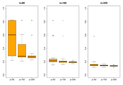
Figure 1: Boxplot of ${1\over 2}\{D({\mathcal{M}}(\widehat{\mathbf{A}}_{1}),{\mathcal{M}}({\mathbf{A}}_{1}))+D({\mathcal{M}}(\widehat{\mathbf{A}}_{2}),{\mathcal{M}}({\mathbf{A}}_{2}))\}$ from a simulation with 100 replications.

Fig.2 presents the boxplots of

$${\rm MSE}(\widehat{\xi})={1\over np}\sum_{t=1}^{n}\sum_{j=1}^{p}\{\widehat{\xi}_{t}({\mathbf{s}}_{j})-\xi_{t}({\mathbf{s}}_{j})\}^{2},\quad{\rm MSE}(\widetilde{\xi})={1\over np}\sum_{t=1}^{n}\sum_{j=1}^{p}\{\widetilde{\xi}_{t}({\mathbf{s}}_{j})-\xi_{t}({\mathbf{s}}_{j})\}^{2},$$ (6.1)

where $\widehat{\xi}_{t}({\mathbf{s}}_{j})$ and $\widetilde{\xi}_{t}({\mathbf{s}}_{j})$ are defined in, respectively, (3.10) and (3.11). We set $J=100$ for the aggregation estimates $\widetilde{\xi}_{t}({\mathbf{s}}_{j})$. As shown by Theorem 1, $\widetilde{\xi}_{t}({\mathbf{s}}_{j})$ always provides more accurate estimate for $\xi_{t}({\mathbf{s}}_{j})$ than $\widehat{\xi}_{t}({\mathbf{s}}_{j})$. Furthermore the MSE decreases when either $n$ or $p$ increases.

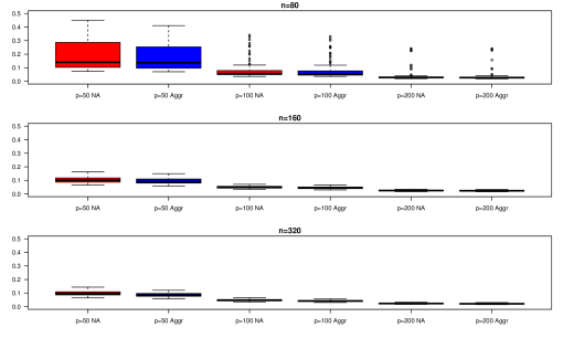
Figure 2: Boxplot of MSE$(\widehat{\xi})$ (red) and MSE$(\widetilde{\xi})$ (blue) in a simulation with 100 replications.

Note that estimating ${\mathbf{A}}_{1},{\mathbf{A}}_{2}$ with $\tau>0$ makes use the continuity of the loading functions $a_{i}(\cdot)$. Table 1 lists the means and the standard errors, over 100 replications, of MSE$(\widehat{\xi})$ with $\widehat{\xi}_{t}({\mathbf{s}}_{j})$ calculated using either $\tau$ selected by the five-fold cross-validation (i.e. $\tau>0$) or $\tau=0$. The improvement from using the continuity is more pronounced when $n$ and $p$ are small.

Table 1: Means and standard errors (in parentheses) of MSE$(\widehat{\xi})$ with $\widehat{\xi}_{t}({\mathbf{s}}_{i})$ calculated using either $\tau>0$ selected by five-fold cross-validation or $\tau=0$.

$n$	$p$	$\tau>0$	$\tau=0$
80	50	0.0941(0.0347)	0.1139 (0.0429)
160	50	0.0665(0.0164)	0.0795 (0.0250)
320	50	0.0585(0.0076)	0.0631 (0.0126)
80	100	0.0243(0.0157)	0.0279 (0.0183)
160	100	0.0158(0.0055)	0.0168 (0.0073)
320	100	0.0146(0.0011)	0.0150 (0.0012)
80	200	0.0056(0.0050)	0.0064 (0.0058)
160	200	0.0039(0.0002)	0.0039 (0.0003)
320	200	0.0037(0.0002)	0.0037 (0.0002)

To illustrate the kriging performance, with each sample we also draw additional 50 ‘post-sample’ data points at the locations randomly drawn from $U[-1,1]^{2}$. For each $t=1,\cdots,n$, we calculate the spatial kriging estimate $\widehat{y}_{t}^{r}(\cdot)$ in (4.9) at each of the 50 post-sample locations. The mean squared predictive error is computed as

$${\rm MSPE}(\widehat{y}^{r})={1\over 50n}\sum_{t=1}^{n}\sum_{{\mathbf{s}}_{0}\in{\mathcal{S}}^{*}}\{\widehat{y}_{t}^{r}({\mathbf{s}}_{0})-y_{t}({\mathbf{s}}_{0})\}^{2},$$ (6.2)

where ${\mathcal{S}}^{*}$ is the set consisting of the 50 post-sample locations. Similarly, we repeat this exercise for $\widetilde{y}_{t}^{r}(\cdot)$ in (4.18). To check the performance of the kriging in time, we also generate two post-sample surfaces at times $n+1$ and $n+2$ for each sample. The mean of square predictive error (${\rm MSPE}$) is calculated as follows.

$${\rm MSPE}(\widehat{y}^{r}_{n+\ell})=\frac{1}{p}\sum_{j=1}^{p}\{\widehat{y}_{n+\ell}^{r}({\mathbf{s}}_{j})-y_{n+\ell}({\mathbf{s}}_{j})\}^{2},\qquad\ell=1,2.$$ (6.3)

We repeat the above exercise for the aggregation estimator $\widetilde{y}^{r}_{n+\ell}$ with $J=100$.

Table 2: Means of $\widehat{d}$, means and standard errors (in parentheses) of MSPE for kriging in space and time.

			Kriging over Space		Kriging in Time
$n$	$p$	$\widehat{d}$	${\rm MSPE}(\widehat{y}^{r}_{t})$	${\rm MSPE}(\tilde{y}^{r}_{t})$	${\rm MSPE}(\widehat{y}^{r}_{t+1})$	${\rm MSPE}(\tilde{y}^{r}_{t+1})$	${\rm MSPE}(\widehat{y}^{r}_{t+2})$	${\rm MSPE}(\tilde{y}^{r}_{t+2})$
80	50	2.03	1.1893(0.1094)	1.1763(0.1030)	1.6300(0.5402)	1.5660(0.5225)	1.7856(0.8940)	1.6876(0.8237)
160	50	2.76	1.1119(0.0553)	1.1016(0.0467)	1.3765(0.4160)	1.3346(0.3952)	1.4795(0.4749)	1.4599(0.4754)
320	50	2.98	1.1004(0.0243)	1.0888(0.0209)	1.5073(0.5175)	1.4699(0.4932)	1.6132(0.7828)	1.5855(0.7640)
80	100	2.62	1.0829(0.0765)	1.0804(0.0735)	1.5037(0.4135)	1.4354(0.3904)	1.8469(0.7127)	1.7680(0.6564)
160	100	2.97	1.0509(0.0283)	1.0455(0.0255)	1.4701(0.4359)	1.4244(0.4119)	1.6118(0.5449)	1.5866(0.5357)
320	100	3.00	1.0462(0.0141)	1.0412(0.0139)	1.3541(0.3580)	1.3290(0.3410)	1.6301(0.6608)	1.6137(0.6555)
80	200	2.88	1.0411(0.0484)	1.0368(0.0457)	1.5157(0.4376)	1.4884(0.4297)	1.8312(0.7495)	1.7954(0.7220)
160	200	3.00	1.0238(0.0146)	1.0221(0.0147)	1.4471(0.4120)	1.4326(0.4211)	1.6841(0.5954)	1.6721(0.5910)
320	200	3.00	1.0225(0.0122)	1.0204(0.0121)	1.4006(0.3285)	1.3877(0.3299)	1.5689(0.5047)	1.5650(0.5111)

The means and the standard errors of the MSPE in the 100 replications for each settings are listed in Table 2. In general MSPE decreases as $n$ increases. For the kriging over space, MSPE also decreases as $p$ increases. See also Theorem 2, noting $\delta=0$ when all the factors are strong. MSPEs of the kriging over space are smaller than those of the kriging in time. This is understandable from comparing Theorem 2 and Theorem 3. The aggregated kriging always outperforms the non-aggregate counterparts. Last but not least, the ratio estimator (3.7) for $d$ works well for reasonably large $n$ and $p$.

6.2 Real Data Analysis

We illustrate the proposed methods with the monthly temperature records (in Celsius) at the 128 monitoring stations in China from January 1970 to December 2000. All series are of the length $n=372$. For each series, we remove the annually seasonal component by subtracting the average temperature of the same months. The distance among the stations are calculated as the great circle distance based on their longitudes and latitudes.

For kriging over space, we randomly select $p=78$ stations for estimation, and predict the values at the other 50 stations. The mean squared predictive error for the non-aggregation estimates (4.8) are calculated as follows.

$${\rm MSPE}(\widehat{y}^{r})={1\over 50\times 372}\sum_{t=1}^{372}\sum_{{\mathbf{s}}_{0}\in{\mathcal{S}}^{*}}\big{\{}\widehat{y}_{t}^{r}({\mathbf{s}}_{0})-y_{t}({\mathbf{s}}_{0})\big{\}}^{2}.$$

We also apply the aggregation (with $J=100$) estimator $\widetilde{y}_{t}(\cdot)$ in (4.18) to improve the kriging accuracy. To avoid the sampling bias in selecting stations, we replicate this exercise 100 times via randomly dividing the 128 stations into two sets of sizes 78 and 50. The estimated $d$-values are equal to 1 in the 98 replications, and are 2 in the two other replications. The means of MSPE over the 100 replications for $\widehat{y}^{r}$ and $\widetilde{y}^{r}$ are 0.7787 and 0.7718, and the corresponding standard errors are 0.0335 and 0.0444, respectively. In the training step, the average MSPE of cross-validation are 0.2407 with optimal $\tau$, where $\tau>0$, and 0.2493 with $\tau$ equals to zero. Among all 100 replications, the optimal $\tau$’s are larger than zero for 93 times.

For kriging in time, we consider one-step-ahead and two-step-ahead post-sample prediction (with $j_{0}=6$) for all the 128 locations in each of the last 24 months in the data set. The corresponding mean squared predictive error at each step is defined as

$${\rm MSPE}(\widehat{y}^{r}_{n+\ell})={1\over 128}\sum_{j=1}^{128}\big{\{}\widehat{y}_{n+\ell}^{r}({\mathbf{s}}_{j})-y_{n+\ell}({\mathbf{s}}_{j})\big{\}}^{2},\qquad\ell=1,2.$$

We also apply the aggregation estimator $\widetilde{y}^{r}_{n+\ell}(\cdot)$ with $J=100$. The means and standard errors of ${\rm MSPE}(\widehat{y}^{r}_{n+\ell})$ over the last 24 months is 1.7338 and 1.2581 for $\ell=1$, while 1.8814 and 1.4680 for $\ell=2$. On the other side, the means and standard errors of ${\rm MSPE}(\widetilde{y}^{r}_{n+\ell})$ are 1.7303 and 1.2583 for $\ell=1$, 1.8802 and 1.4673 for $\ell=2$, respectively. As we expected, the one-step-ahead prediction is more accurate than the two-step-ahead prediction.

Overall the kriging in space is more accurate than those in time. The aggregation via random partitioning of locations improves the prediction, though the improvement is not substantial in this example.

Acknowledgements. We thank Professor Noel Cressie for helpful comments and suggestions.

References

Banerjee, S., Gelfand, A., Finley, A. O. and Sang, H. (2008). Gaussian predictive process models for large spatial data sets. Journal of the Royal Statistical Society, B, 70, 825-848.

Bathia, N., Yao, Q. and Ziegelmann, F. (2010). Identifying the finite dimensionality of curve time series. The Annals of Statistics, 38, 3352-3386.

Breiman, L. (1996). Bagging predictors. Machine Learning, 24, 123-140.

Castruccio, S. and Stein, M. L. (2013). Global space-time models for climate ensembles. Annals of Applied Statistics, 7, 1593-1611.

Chang, J., Guo, B. and Yao, Q. (2015). High dimensional stochastic regression with latent factors, endogeneity and nonlinearity. Journal of Econometrics, 189, 297-312.

Cressie, N. and Johannesson, G. (2008). Fixed rank kriging for very large spatial data sets. Journal of the Royal Statistical Society, B, 70, 209-226.

Cressie, N., Shi, T. and Kang, E.L. (2010). Fixed rank filtering for spatio-temporal data. Journal of Computational and Graphical Statistics, 19, 724-745.

Cressie, N. and Wikle, C. K. (2011). Statistics for Spatio-Temporal Data. Wiley, Hoboken.

Fan, J. and Gijbels, I. (1996). Local Polynomial Modelling and Its Applications. Chapman and Hall, London.

Finley, A., Sang, H., Banerjee, S. and Gelfand, A. (2009). Improving the performance of predictive process modeling for large datasets. Computational Statistics and Data Analysis, 53, 2873-2884.

Gneiting, T. (2002). Compactly supported correlation functions. Journal of Multivariate Analysis, 83, 493-508.

Golub, G. and Van Loan, C. (1996). Matrix Computations (3rd edition). John Hopkins University Press.

Guinness, J. and Stein, M. L. (2013). Interpolation of nonstationary high frequency spatial-temporal temperature data. Annals of Applied Statistics, 7, 1684-1708.

Hall, P., Fisher, N. I., and Hoffmann, B. (1994). On the Nonparametric Estimation of Covariance Functions. The Annals of Statistics, 22, 2115-2134.

Hastie, T., Tibshirani, R. and Friedman, J. (2009). The Elements of Statistical Learning. Springer, New York.

Higdon, D. (2002). Space and space-time modeling using process convolutions. In Quantitative Methods for Current Environmental Issues (eds C. W. Anderson, V. Barnett, P. C. Chatwin and A. H. El-Shaarawi), pp. 37-54. London: Springer.

Jun, M. and Stein, M. L. (2007). An approach to producing space-time covariance functions on spheres. Technometrics, 49, 468-479.

Kammann, E. E. and Wand, M. P. (2003). Geoadditive models. Applied Statistics, 52, 1-18.

Katzfuss, M. and Cressie, N. (2011). Spatio-temporal smoothing and EM estimation for massive remote-sensing data sets. Journal of Time Series Analysis, 32, 430-446.

Kaufman, C., Schervish, M. and Nychka, D. (2008). Covariance tapering for likelihood-based estimation in large spatial data sets. Journal of the American Statistical Association, 103, 1545-1555.

Lam, C. and Yao, Q. (2012). Factor modelling for high-dimensional time series: inference for the number of factors. The Annals of Statistics, 40, 694-726

Lam, C., Yao, Q. and Bathia, N. (2011). Estimation for latent factors for high-dimensional time series. Biometrika, 98, 901-918.

Li, B., Genton, M. G. and Sherman, M. (2007). A nonparametric assessment of properties of space-time covariance functions. Journal of the American Statistical Association, 102, 736-744.

Lin, Z. and Lu, C. (1996). Limit Theory on Mixing Dependent Random Variables. Kluwer Academic Publishers, New York.

Mercer, J. (1909). Functions of positive and negative type and their connection with the theory of integral equations. Philosophical Transactions of the Royal Society A, 209, 415-446.

Sang, H. and Huang J. Z. (2012). A full-scale approximation of covariance functions for large spatial data sets. Journal of the Royal Statistical Society, B, 74, 111-132.

Smith, R. L., Kolenikov, S. and Cox, L. H. (2003). Spatiotemporal modelling of PM_2.5 data with missing values. Journal of Geophysical Research, 108, No.D24, DOI:10.1029/2002JD002914.

Stein, M. (2008). A modeling approach for large spatial data sets. Journal of the Korean Statistical Society, 37, 3-10.

Tzeng, S.L. and Huang, H.C. (2018). Resolution adaptive fixed rank kriging. Technometrics, to appear.

Wang, W.T. and Huang, H.C. (2017). Regularized principal component analysis for spatial data. Journal of Computational and Graphical Statistics, 26, 14-25.

Wikle, C. and Cressie, N. (1999). A dimension-reduced approach to space-time Kalman filtering. Biometrika, 86, 815-829.

Zhang, B., Sang, H., Huang, J. Z. (2015). Full-scale approximations of spatio-temporal covariance models for large datasets. Statistica Sinica, 25, 99-114.

Zhang, R., Robinson, P. and Yao, Q. (2018). Identifying cointegration by eigenanalysis. Available at arXiv:1505.00821.

Zhu, H., Fan, J. and Kong, L. (2014). Spatially varying coefficient model for neuroimaging data with jump discontinuities. Journal of the American Statistical Association, 109, 1084-1098.

Supplementary document of “Krigings over space and time based on latent low-dimensional structures”

Appendix: Technical proofs

Proof of Proposition 1. The first part of the proposition can be proved in the same manner as Proposition 1 of Bathia et al. (2010), which is omitted. To prove the second part, it follows (2.9) and (2.8) that any eigenfunction of $\Sigma_{0}$ must be the linear combination of $a_{1},\cdots,a_{d}$, i.e. $\varphi_{i}({\mathbf{s}})=\sum_{j}\gamma_{ij}a_{j}({\mathbf{s}})$. Now it follows from (2.11) and (2.8) that

$$\Sigma_{0}\circ\varphi_{i}({\mathbf{s}}) =\sum_{k,\ell,j}\sigma_{k\ell}\gamma_{ij}a_{k}({\mathbf{s}})\mbox{$\langle a_{\ell},a_{j}\rangle$}=\sum_{k,j}\sigma_{kj}\gamma_{ij}a_{k}({\mathbf{s}})=\sum_{k}\lambda_{i}\gamma_{ik}a_{k}({\mathbf{s}})=\lambda_{i}\varphi_{i}({\mathbf{s}}).$$

Since $a_{1},\cdots,a_{d}$ are orthonormal, it must hold that

$$\sum_{j}\sigma_{kj}\gamma_{ij}=\lambda_{i}\gamma_{ik},\qquad k=1,\cdots,d.$$ (A.1)

As $\sigma_{kj}$ is the $(k,j)$-th element of matrix $\mbox{Var}({\mathbf{x}}_{t})$, (A.1) is equivalent to $\mbox{Var}({\mathbf{x}}_{t})\boldsymbol{\gamma}_{i}=\lambda_{i}\boldsymbol{\gamma}_{i}$, i.e. $\boldsymbol{\gamma}_{i}$ is an eigenvector of $\mbox{Var}({\mathbf{x}}_{t})$ corresponding to the eigenvalue $\lambda_{i}$, $i=1,\cdots,d$. Furthermore,

$$I(i=k)=\mbox{$\langle\phi_{i},\phi_{k}\rangle$}=\sum_{j,\ell}\gamma_{ij}\gamma_{k\ell}\mbox{$\langle a_{j},a_{\ell}\rangle$}=\sum_{j}\gamma_{ij}\gamma_{kj}=\boldsymbol{\gamma}_{i}^{\prime}\boldsymbol{\gamma}_{k}.$$

Thus $\boldsymbol{\gamma}_{1},\cdots,\boldsymbol{\gamma}_{d}$ are orthogonal. $\blacksquare$

To prove Theorem 1(ii), we first introduce Lemma 3 below. For the simplicity in presentation, we assume that the $d$ positive eigenvalues of $\boldsymbol{\Sigma}\boldsymbol{\Sigma}^{\prime}$, defined in (3.5), are distinct from each other. Then both ${\mathbf{A}}_{1}$ and ${\mathbf{A}}_{2}$ are uniquely defined if we line up each of the two sets of the $d$ orthonormal eigenvectors (i.e. the columns of ${\mathbf{A}}_{1}$ and ${\mathbf{A}}_{2}$) in the descending order of their corresponding eigenvalues, and we require that the first non-zero element of each those eigenvector to be positive. See the discussion below (3.5) above.

Using the same notation as in (3.8), we denote by $\widehat{\mathbf{A}}_{1}^{(j)},\,\widehat{\mathbf{A}}_{2}^{(j)}$ the estimated factor loading matrices in (3.8) with the $j$-th partition, by $\boldsymbol{\Sigma}^{(j)}$ the covariance matrix in (3.4), and by ${\mathbf{x}}_{t}^{(j)},\,{\mathbf{x}}_{t}^{*(j)}$ the estimated latent factors in (3.9), $j=1,\cdots,p_{0}=p!/(p_{1}!p_{2}!)$. Assume that the $d$ positive eigenvalues of $\boldsymbol{\Sigma}^{(j)}(\boldsymbol{\Sigma}^{(j)})^{\prime}$ are distinct. Then $\widehat{\mathbf{A}}_{1}^{(j)}$ and $\widehat{\mathbf{A}}_{2}^{(j)}$ can be uniquely defined as above. Now we are ready to state the lemma.

Lemma 3

Let Condition 1 hold. Let the $d$ positive eigenvalues of $\boldsymbol{\Sigma}^{(j)}(\boldsymbol{\Sigma}^{(j)})^{\prime}$ be distinct, and Condition 2 hold for ${\mathbf{x}}_{t}^{(j)}$ and ${\mathbf{x}}_{t}^{*(j)}$ for all $j=1,\cdots,p_{0}$. Then as $p^{\delta}n^{-1/2}+p^{2\delta-2}\tau\|{\mathbf{L}}\|=o(1)$, it holds that

$$\max_{1\leq j\leq p_{0}}\{||\widehat{\mathbf{A}}_{1}^{(j)}-{\mathbf{A}}_{1}^{(j)}||+||\widehat{\mathbf{A}}_{2}^{(j)}-{\mathbf{A}}_{2}^{(j)}||\}=O_{P}(p^{\delta}n^{-1/2}+p^{2\delta-2}\tau\|{\mathbf{L}}\|).$$

Proof. Since $\max_{1\leq j\leq p_{0}}||\widehat{\mathbf{A}}_{2}^{(j)}-{\mathbf{A}}_{2}^{(j)}||$ can be shown similarly to $\max_{1\leq j\leq p_{0}}||\widehat{\mathbf{A}}_{1}^{(j)}-{\mathbf{A}}_{1}^{(j)}||$, we only prove $\max_{1\leq j\leq p_{0}}||\widehat{\mathbf{A}}_{1}^{(j)}-{\mathbf{A}}_{1}^{(j)}||$ here. Note that for any $1\leq j\leq p_{0}$,

$$||\widehat{\boldsymbol{\Sigma}}^{(j)}(\widehat{\boldsymbol{\Sigma}}^{(j)})^{\prime}-\tau{\mathbf{L}}-\boldsymbol{\Sigma}^{(j)}(\boldsymbol{\Sigma}^{(j)})^{\prime}||\leq||\widehat{\boldsymbol{\Sigma}}^{(j)}-\boldsymbol{\Sigma}^{(j)}||^{2}+2||\boldsymbol{\Sigma}^{(j)}||\times||\widehat{\boldsymbol{\Sigma}}^{(j)}-\boldsymbol{\Sigma}^{(j)}||+\tau\|{\mathbf{L}}\|.$$ (A.2)

Since ${\mathbf{x}}_{t}^{(j)}$ satisfies Condition 2, it follows that $||\boldsymbol{\Sigma}^{(j)}||=O(p^{1-\delta}),$ see Lam et al. (2011). On the other hand, by the mixing condition of $\{{\mathbf{y}}_{t}\}$, we have

$$\sup_{j}||\widehat{\boldsymbol{\Sigma}}^{(j)}-\boldsymbol{\Sigma}^{(j)}||^{2} = \sup_{j}||{1\over n}\sum_{t=1}^{n}\{({\mathbf{y}}_{t,1}^{(j)}-\bar{\mathbf{y}}_{1}^{(j)})({\mathbf{y}}_{t,2}^{(j)}-\bar{\mathbf{y}}_{2}^{(j)})^{\prime}-\mathrm{Cov}({\mathbf{y}}_{t,1}^{(j)},{\mathbf{y}}_{t,2}^{(j)})\}||^{2}$$

$$\leq \sum_{i=1}^{p}\sum_{j=1}^{p}\Big{\{}{1\over n}\sum_{t=1}^{n}[y_{t}({\mathbf{s}}_{i})-\bar{y}({\mathbf{s}}_{i})][y_{t}({\mathbf{s}}_{j})-\bar{y}({\mathbf{s}}_{j})]-\hbox{Cov}[y_{t}({\mathbf{s}}_{i}),y_{t}({\mathbf{s}}_{j})]\Big{\}}^{2}$$

$$= O_{p}(p^{2}/n).$$

Thus, by (A.2),

$$\sup_{j}||\widehat{\boldsymbol{\Sigma}}^{(j)}(\widehat{\boldsymbol{\Sigma}}^{(j)})^{\prime}-\tau{\mathbf{L}}-\boldsymbol{\Sigma}^{(j)}(\boldsymbol{\Sigma}^{(j)})^{\prime}||=O_{p}(p^{2-\delta}n^{-1/2}+\tau\|{\mathbf{L}}\|).$$ (A.3)

By (A.3) and a similar argument to Theorem 1 of Lam et al. (2011), we can show that

$$\max_{1\leq j\leq p_{0}}||\widehat{\mathbf{A}}_{1}^{(j)}-{\mathbf{A}}_{1}^{(j)}||=O_{P}(p^{\delta}n^{-1/2}+p^{2\delta-2}\tau\|{\mathbf{L}}\|)$$

and complete the proof of Lemma 3. $\blacksquare$

Proof of Theorem 1(ii). Note that

$$\mathrm{E}\Big{[}{1\over np}\sum_{t=1}^{n}\sum_{i=1}^{p}\big{\{}\widehat{\xi}_{t}({\mathbf{s}}_{i})-\xi_{t}({\mathbf{s}}_{i})\big{\}}^{2}\Big{|}\{\xi_{t}({\mathbf{s}}_{i}),\,y_{t}({\mathbf{s}}_{i})\}\Big{]}$$

$$= {1\over npp_{0}}\sum_{t=1}^{n}\sum_{j=1}^{p_{0}}[\widehat{\mathbf{A}}_{1}^{(j)}\widehat{\mathbf{x}}_{t}^{(j)}-{\mathbf{A}}_{1}^{(j)}{\mathbf{x}}_{t}^{(j)}]^{\prime}[\widehat{\mathbf{A}}_{1}^{(j)}\widehat{\mathbf{x}}_{t}^{(j)}-{\mathbf{A}}_{1}^{(j)}{\mathbf{x}}_{t}^{(j)}]$$

$$+{1\over npp_{0}}\sum_{t=1}^{n}\sum_{j=1}^{p_{0}}[\widehat{\mathbf{A}}_{2}^{(j)}\widehat{\mathbf{x}}_{t}^{*(j)}-{\mathbf{A}}_{2}^{(j)}{\mathbf{x}}_{t}^{*(j)}]^{\prime}[\widehat{\mathbf{A}}_{2}^{(l)}\widehat{\mathbf{x}}_{t}^{*(j)}-{\mathbf{A}}_{2}^{(j)}{\mathbf{x}}_{t}^{*(j)}]$$

$$\equiv \Sigma_{1}+\Sigma_{2}.$$

By Lemma 3, we have

$$\Sigma_{1} = {1\over npp_{0}}\sum_{t=1}^{n}\sum_{j=1}^{p_{0}}\Big{\{}[\widehat{\mathbf{A}}_{1}^{(j)}(\widehat{\mathbf{A}}_{1}^{(j)})^{\prime}-{\mathbf{A}}_{1}^{(j)}({\mathbf{A}}_{1}^{(j)})^{\prime}]{\mathbf{A}}_{1}^{(j)}{\mathbf{x}}_{t}^{(j)}+\widehat{\mathbf{A}}_{1}^{(j)}(\widehat{\mathbf{A}}_{1}^{(j)})^{\prime}{\varepsilon}_{t,1}^{(j)}\Big{\}}^{\prime}$$ (A.4)

$$\Big{\{}[\widehat{\mathbf{A}}_{1}^{(j)}(\widehat{\mathbf{A}}_{1}^{(j)})^{\prime}-{\mathbf{A}}_{1}^{(j)}({\mathbf{A}}_{1}^{(j)})^{\prime}]{\mathbf{A}}_{1}^{(j)}{\mathbf{x}}_{t}^{(j)}+\widehat{\mathbf{A}}_{1}^{(j)}(\widehat{\mathbf{A}}_{1}^{(j)})^{\prime}{\varepsilon}_{t,1}^{(j)}\Big{\}}^{\prime}$$

$$= {1\over npp_{0}}\sum_{t=1}^{n}\sum_{j=1}^{p_{0}}({\mathbf{x}}_{t}^{(j)})^{\prime}(\widehat{\mathbf{A}}_{1}^{(j)})^{\prime}[\widehat{\mathbf{A}}_{1}^{(j)}(\widehat{\mathbf{A}}_{1}^{(j)})^{\prime}-{\mathbf{A}}_{1}^{(j)}({\mathbf{A}}_{1}^{(j)})^{\prime}]^{\prime}[\widehat{\mathbf{A}}_{1}^{(j)}(\widehat{\mathbf{A}}_{1}^{(j)})^{\prime}-{\mathbf{A}}_{1}^{(j)}({\mathbf{A}}_{1}^{(j)})^{\prime}]{\mathbf{A}}_{1}^{(j)}{\mathbf{x}}_{t}^{(j)}$$

$$+{1\over npp_{0}}\sum_{t=1}^{n}\sum_{j=1}^{p_{0}}({\mathbf{x}}_{t}^{(j)})^{\prime}({\mathbf{A}}_{1}^{(j)})^{\prime}[\widehat{\mathbf{A}}_{1}^{(j)}(\widehat{\mathbf{A}}_{1}^{(j)})^{\prime}-{\mathbf{A}}_{1}^{(j)}({\mathbf{A}}_{1}^{(j)})^{\prime}]^{\prime}\widehat{\mathbf{A}}_{1}^{(j)}(\widehat{\mathbf{A}}_{1}^{(j)})^{\prime}{\varepsilon}_{t,1}^{(j)}$$

$$+{1\over npp_{0}}\sum_{t=1}^{n}\sum_{j=1}^{p_{0}}({\varepsilon}_{t,1}^{(j)})^{\prime}\widehat{\mathbf{A}}_{1}^{(j)}(\widehat{\mathbf{A}}_{1}^{(j)})^{\prime}[\widehat{\mathbf{A}}_{1}^{(j)}(\widehat{\mathbf{A}}_{1}^{(j)})^{\prime}-{\mathbf{A}}_{1}^{(j)}({\mathbf{A}}_{1}^{(j)})^{\prime}]{\mathbf{A}}_{1}^{(j)}{\mathbf{x}}_{t}^{(j)}$$

$$+{1\over npp_{0}}\sum_{t=1}^{n}\sum_{j=1}^{p_{0}}({\varepsilon}_{t,1}^{(j)})^{\prime}\widehat{\mathbf{A}}_{1}^{(j)}(\widehat{\mathbf{A}}_{1}^{(j)})^{\prime}\widehat{\mathbf{A}}_{1}^{(j)}(\widehat{\mathbf{A}}_{1}^{(j)})^{\prime}{\varepsilon}_{t,1}^{(j)}$$

$$= O_{p}(p^{\delta}/n+p^{(\delta-1)/2}n^{-/2}+p^{\delta-2}\tau\|{\mathbf{L}}\|)+{1\over npp_{0}}\sum_{t=1}^{n}\sum_{j=1}^{p_{0}}({\varepsilon}_{t,1}^{(j)})^{\prime}{\mathbf{A}}_{1}^{(j)}({\mathbf{A}}_{1}^{(j)})^{\prime}{\varepsilon}_{t,1}^{(j)}.$$

Since $\mathrm{E}\Big{(}{1\over p_{0}}\sum_{j=1}^{p_{0}}({\varepsilon}_{t,1}^{(j)})^{\prime}{\mathbf{A}}_{1}^{(j)}({\mathbf{A}}_{1}^{(j)})^{\prime}{\varepsilon}_{t,1}^{(j)}\Big{)}^{2}\leq{1\over p_{0}}\sum_{j=1}^{p_{0}}\mathrm{E}\Big{[}({\varepsilon}_{t,1}^{(j)})^{\prime}{\mathbf{A}}_{1}^{(j)}({\mathbf{A}}_{1}^{(j)})^{\prime}{\varepsilon}_{t,1}^{(j)}\Big{]}^{2}<\infty,$ it follows from Markov’s inequality that

$${1\over np_{0}}\sum_{t=1}^{n}\sum_{j=1}^{p_{0}}({\varepsilon}_{t,1}^{(j)})^{\prime}{\mathbf{A}}_{1}^{(j)}({\mathbf{A}}_{1}^{(j)})^{\prime}{\varepsilon}_{t,1}^{(j)}\stackrel{{\scriptstyle p}}{{\longrightarrow}}\mathrm{E}\Big{[}({\varepsilon}_{t,1}^{(j)})^{\prime}{\mathbf{A}}_{1}^{(j)}({\mathbf{A}}_{1}^{(j)})^{\prime}{\varepsilon}_{t,1}^{(j)}\Big{]}.$$

Thus, by (Supplementary document of “Krigings over space and time based on latent low-dimensional structures”), we have the following two conclusions:

• When $n\rightarrow\infty$, $\Sigma_{1}=O_{p}(p^{\delta}/n+p^{(\delta-1)/2}n^{-/2}+p^{\delta-2}\tau\|{\mathbf{L}}\|+p^{-1}).$

• When $p^{1+\delta}/n+p^{\delta-1}\tau\|{\mathbf{L}}\|\rightarrow 0$, $p\Sigma_{1}\stackrel{{\scriptstyle p}}{{\longrightarrow}}\mathrm{E}\Big{[}({\varepsilon}_{t,1}^{(1)})^{\prime}{\mathbf{A}}_{1}^{(1)}({\mathbf{A}}_{1}^{(1)})^{\prime}{\varepsilon}_{t,1}^{(1)}\Big{]}.$

Similarly, the above properties hold also for $\Sigma_{2}.$ Hence,

$$\mathrm{E}\Big{[}{1\over np}\sum_{t=1}^{n}\sum_{i=1}^{p}\big{\{}\widehat{\xi}_{t}({\mathbf{s}}_{i})-\xi_{t}({\mathbf{s}}_{i})\big{\}}^{2}\Big{|}\{\xi_{t}({\mathbf{s}}_{i}),\,y_{t}({\mathbf{s}}_{i})\}\Big{]}=O_{p}(p^{\delta}/n+p^{(\delta-1)/2}n^{-/2}+p^{\delta-2}\tau\|{\mathbf{L}}\|+p^{-1}).\,\,\,$$ (A.5)

Further, when $p^{1+\delta}/n+p^{\delta-1}\tau\|{\mathbf{L}}\|\rightarrow 0$,

$$\mathrm{E}\Big{[}{1\over n}\sum_{t=1}^{n}\sum_{i=1}^{p}\big{\{}\widehat{\xi}_{t}({\mathbf{s}}_{i})-\xi_{t}({\mathbf{s}}_{i})\big{\}}^{2}\Big{|}\{\xi_{t}({\mathbf{s}}_{i}),\,y_{t}({\mathbf{s}}_{i})\}\Big{]}=\mathrm{E}\Big{[}({\varepsilon}_{t,1}^{(1)})^{\prime}{\mathbf{A}}_{1}^{(1)}({\mathbf{A}}_{1}^{(1)})^{\prime}{\varepsilon}_{t,1}^{(1)}+({\varepsilon}_{t,2}^{(1)})^{\prime}{\mathbf{A}}_{2}^{(1)}({\mathbf{A}}_{2}^{(1)})^{\prime}{\varepsilon}_{t,2}^{(1)}\Big{]}$$

in probability. $\blacksquare$

Lemma 4

Let Condition 1 hold and $pn^{-\beta/2}\rightarrow 0$. Then

$$\lim_{n\rightarrow\infty}P\left\{\min_{1\leq i\leq p}\lambda_{\min}[n^{-1}{\mathbf{Z}}({\mathbf{s}}_{i})^{\prime}{\mathbf{Z}}({\mathbf{s}}_{i})]\geq c_{0}/2\right\}=1.$$

Proof. Let $z_{t}^{j}({\mathbf{s}}_{i}),\,j=1,\cdots,m$ be the components of ${\mathbf{z}}_{t}({\mathbf{s}}_{i}).$ Since $\{{\mathbf{z}}_{t}({\mathbf{s}}_{i})\}$ is a stationary $\alpha$-mixing process satisfying Condition 1, by Lemma 12.2.2 of Lin and Lu (1996), we have that for any $1\leq j,k\leq m$,

$$\mathrm{E}\left|{1\over n}\sum_{t=1}^{n}\{z_{t}^{j}({\mathbf{s}}_{i})z_{t}^{k}({\mathbf{s}}_{i})-\mathrm{E}[z_{t}^{j}({\mathbf{s}}_{i})z_{t}^{k}({\mathbf{s}}_{i})]\}\right|^{\beta}=O(n^{-\beta/2}).$$ (A.6)

Since $m$ is finite, it follows that

$$\mathrm{E}||n^{-1}{\mathbf{Z}}({\mathbf{s}}_{i})^{\prime}{\mathbf{Z}}({\mathbf{s}}_{i})-\hbox{Var}({\mathbf{z}}_{t}({\mathbf{s}}_{i}))||_{F}^{\beta}=O(n^{-\beta/2}),$$ (A.7)

where $||\cdot||_{F}$ denotes the Frobenius norm. Now suppose that $\min_{1\leq i\leq p}\lambda_{\min}[n^{-1}{\mathbf{Z}}({\mathbf{s}}_{i})^{\prime}{\mathbf{Z}}({\mathbf{s}}_{i})]<c_{0}/2$. Since $\min_{1\leq i\leq p}\lambda_{\min}[\hbox{Var}({\mathbf{z}}_{t}({\mathbf{s}}_{i}))]>c_{0}$, and

$$\hbox{Var}({\mathbf{z}}_{t}({\mathbf{s}}_{i}))=[\hbox{Var}({\mathbf{z}}_{t}({\mathbf{s}}_{i}))-n^{-1}{\mathbf{Z}}({\mathbf{s}}_{i})^{\prime}{\mathbf{Z}}({\mathbf{s}}_{i})]+n^{-1}{\mathbf{Z}}({\mathbf{s}}_{i})^{\prime}{\mathbf{Z}}({\mathbf{s}}_{i}),$$

it must hold that

$$\max_{1\leq i\leq p}||n^{-1}{\mathbf{Z}}({\mathbf{s}}_{i})^{\prime}{\mathbf{Z}}({\mathbf{s}}_{i})-\hbox{Var}({\mathbf{z}}_{t}({\mathbf{s}}_{i}))||_{F}\geq c_{0}/2.$$ (A.8)

However, by (A.7), it follows that

$$P\{\max_{1\leq i\leq p}||n^{-1}{\mathbf{Z}}({\mathbf{s}}_{i})^{\prime}{\mathbf{Z}}({\mathbf{s}}_{i})-\hbox{Var}({\mathbf{z}}_{t}({\mathbf{s}}_{i}))||_{F}\geq c_{0}/2\} \leq \sum_{i=1}^{p}(c_{0}/2)^{-\beta}\mathrm{E}||n^{-1}{\mathbf{z}}({\mathbf{s}}_{i})^{\prime}{\mathbf{z}}({\mathbf{s}}_{i})-\hbox{Var}({\mathbf{z}}({\mathbf{s}}_{i}))||_{F}^{\beta}$$ (A.9)

$$= O_{p}(pn^{-\beta/2})=o(1).$$

This implies that $P\{\min_{1\leq i\leq p}\lambda_{\min}[n^{-1}{\mathbf{z}}({\mathbf{s}}_{i})^{\prime}{\mathbf{z}}({\mathbf{s}}_{i})]<c_{0}/2\}=o(1)$ and completes the proof of Lemma 4. $\blacksquare$

theorem and Theorem 8.1.10 of Golub and Van Loan (1996) (see also Lemma 3 of Lam et al. (2011)). (ii) can be shown similarly to Theorem 1 of Bathia, et al. (2010), see also Theorem 1 of Lam and Yao (2012).

Proof for the convergence rate of $\widehat{\boldsymbol{\beta}}({\mathbf{s}}_{0})$. Let $e_{t}({\mathbf{s}})=y_{t}({\mathbf{s}})-{\mathbf{z}}_{t}({\mathbf{s}})^{\prime}\boldsymbol{\beta}({\mathbf{s}})$ and $w_{i}=K_{h}({\mathbf{s}}_{i}-{\mathbf{s}}_{0})/\sum_{i=1}^{p}K_{h}({\mathbf{s}}_{i}-{\mathbf{s}}_{0})$. Then ${\mathbf{e}}({\mathbf{s}})=(e_{1}({\mathbf{s}}),\cdots,e_{n}({\mathbf{s}}))^{\prime}$ and

$$\widehat{\boldsymbol{\beta}}({\mathbf{s}}_{0})=\sum_{i=1}^{p}[{\mathbf{Z}}({\mathbf{s}}_{i})^{\prime}{\mathbf{Z}}({\mathbf{s}}_{i})]^{-1}[{\mathbf{Z}}({\mathbf{s}}_{i})^{\prime}{\mathbf{e}}({\mathbf{s}}_{i})]w_{i}+\sum_{i=1}^{p}\boldsymbol{\beta}({\mathbf{s}}_{i})w_{i}\equiv I_{1}+I_{2}.$$

For any twice differentiable function $g({\mathbf{s}})=g(s_{1},s_{2}),\,{\mathbf{s}}=(s_{1},s_{2})\in\mathcal{R}^{2}$, define $g_{1\cdot}({\mathbf{s}})=\partial g({\mathbf{s}})/\partial s_{1},$ $\,\,g_{\cdot 2}({\mathbf{s}})=\partial g({\mathbf{s}})/\partial s_{2},$ $g_{11}({\mathbf{s}})=\partial^{2}g({\mathbf{s}})/(\partial s_{1})^{2}$ and $g_{22}({\mathbf{s}})=\partial^{2}g({\mathbf{s}})/(\partial s_{2})^{2}$. Under Conditions 3, 4 and Taylor’s expansion, it can be shown that as $p\rightarrow\infty$,

$$I_{2}-\boldsymbol{\beta}({\mathbf{s}}_{0}) = \sum_{i=1}^{p}(\boldsymbol{\beta}({\mathbf{s}}_{i})-\boldsymbol{\beta}({\mathbf{s}}_{0}))w_{i}$$ (A.10)

$$= {h^{2}\over f({\mathbf{s}}_{0})}[\boldsymbol{\beta}_{1\cdot}({\mathbf{s}}_{0})f_{1\cdot}({\mathbf{s}}_{0})+{1\over 2}f({\mathbf{s}}_{0})\boldsymbol{\beta}_{11}({\mathbf{s}}_{0})]\int_{R}\int_{R}x^{2}K(x,y)\,dxdy$$

$$+{h^{2}\over f({\mathbf{s}}_{0})}[\boldsymbol{\beta}_{\cdot 2}({\mathbf{s}}_{0})f_{\cdot 2}({\mathbf{s}}_{0})+{1\over 2}f({\mathbf{s}}_{0})\boldsymbol{\beta}_{22}({\mathbf{s}}_{0})]\int_{R}\int_{R}y^{2}K(x,y)\,dxdy+o(h^{2}).\quad$$

As for $I_{1}$, by Hölder’s inequality, it follows that

$$||I_{1}|| \leq \Big{(}\max_{1\leq i\leq p}\|[{{\mathbf{Z}}({\mathbf{s}}_{i})^{\prime}{\mathbf{Z}}({\mathbf{s}}_{i})/n}]^{-1}\|_{F}\Big{)}\sum_{i=1}^{p}\|{\mathbf{Z}}({\mathbf{s}}_{i})^{\prime}{\mathbf{e}}({\mathbf{s}}_{i})/n\|w_{i}.\,\,$$ (A.11)

By Lemma 4, we have $\max_{1\leq i\leq p}\lambda_{max}\{(n^{-1}{\mathbf{Z}}({\mathbf{s}}_{i})^{\prime}{\mathbf{Z}}({\mathbf{s}}_{i}))^{-1}\}\leq 2/c_{0}$ holds in probability. Since the dimension of ${\mathbf{z}}_{t}({\mathbf{s}})$ is fixed, it follows that

$$\max_{1\leq i\leq p}||(n^{-1}{\mathbf{Z}}({\mathbf{s}}_{i})^{\prime}{\mathbf{Z}}({\mathbf{s}}_{i}))^{-1}||_{F}\leq c_{1}$$ (A.12)

holds in probability for some positive constant $c_{1}$. On the other hand, it is easy to get that

$$\max_{1\leq i\leq p}\mathrm{E}||n^{-1}{\mathbf{Z}}({\mathbf{s}}_{i})^{\prime}{\mathbf{e}}({\mathbf{s}}_{i})||=O(n^{-1/2}),$$

hence,

$$\mathrm{E}\Big{[}\sum_{i=1}^{p}||n^{-1}{\mathbf{Z}}({\mathbf{s}}_{i})^{\prime}{\mathbf{e}}({\mathbf{s}}_{i})||w_{i}\Big{]}=O(n^{-1/2}).$$ (A.13)

It follows from (A.11), (A.12) and (A.13) that

$$||I_{1}||=O_{p}(n^{-1/2}).$$ (A.14)

Thus, by (A.10) and (A.13), we have $|\widehat{\boldsymbol{\beta}}({\mathbf{s}}_{0})-\boldsymbol{\beta}({\mathbf{s}}_{0})|=O_{p}(h^{2}+n^{-1/2}).$ $\blacksquare$

Proof of Theorem 2. Let ${\mathbf{x}}_{t}^{o}={\mathbf{x}}_{t}I({\mathbf{s}}_{i}\in{\cal{S}}_{1})+{\mathbf{x}}_{t}^{*}I({\mathbf{s}}_{i}\in{\cal{S}}_{2}).$ Then

$$\widehat{\xi}_{t}({\mathbf{s}}_{0})-\xi_{t}({\mathbf{s}}_{0}) = \sum_{i=1}^{p}(\widehat{\mathbf{a}}^{\prime}({\mathbf{s}}_{i})\widehat{\mathbf{x}}_{t}^{o}-{\mathbf{a}}^{\prime}({\mathbf{s}}_{i}){\mathbf{x}}_{t}^{o})w_{i}+\sum_{j=1}^{d}\sum_{i=1}^{p}(a_{j}({\mathbf{s}}_{i})-a_{j}({\mathbf{s}}_{0}))x_{tj}^{o}w_{i}$$ (A.15)

$$\equiv J_{1}+J_{2}.$$

Similar to (A.10), we have

$$\left|\sum_{i=1}^{p}[(a_{j}({\mathbf{s}}_{i})-a_{j}({\mathbf{s}}_{0}))/||a({\mathbf{s}}_{0})||]w_{i}\right|=O(h^{2}),$$

which implies that

$$|J_{2}|=O(h^{2})(||{\mathbf{a}}({\mathbf{s}}_{0})||)\sum_{j=1}^{d}|x_{tj}^{o}|=O(dh^{2}\cdot||{\mathbf{a}}({\mathbf{s}}_{0})||\cdot||{\mathbf{x}}_{t}^{o}||)=O_{p}(h^{2}),$$ (A.16)

where we use the fact that $||{\mathbf{x}}_{t}^{o}||=O_{p}(p^{(1-\delta)/2})$ and $||{\mathbf{a}}({\mathbf{s}}_{0})||=O(p^{(\delta-1)/2})$, which is followed by $\lambda_{\min}\{\mathrm{E}({\mathbf{x}}_{t}^{o}({\mathbf{x}}_{t}^{o})^{\prime})\}\asymp p^{1-\delta}$ and

$$(||{\mathbf{a}}({\mathbf{s}}_{0})||^{2})\lambda_{\min}\{\mathrm{E}({\mathbf{x}}_{t}^{o}({\mathbf{x}}_{t}^{o})^{\prime})\}\leq(||{\mathbf{a}}({\mathbf{s}}_{0})||^{2})\mathrm{E}[({\mathbf{a}}^{\prime}({\mathbf{s}}_{0})/||{\mathbf{a}}({\mathbf{s}}_{0})||){\mathbf{x}}_{t}^{o}]^{2}=\mathrm{E}[{\mathbf{a}}^{\prime}({\mathbf{s}}_{0}){\mathbf{x}}_{t}^{o}]^{2}=\mathrm{E}y_{t}^{2}({\mathbf{s}}_{0})<\infty.$$

By (iii) of Proposition 3 and the same arguments as in Theorem 2.2 of Chang et al. (2015), we have that for $i=1,2$,

$$p^{-1/2}||\widehat{\mathbf{A}}_{i}\widehat{\mathbf{x}}_{t}^{o}-{\mathbf{A}}_{i}{\mathbf{x}}_{t}^{o}||=O_{p}(||\widehat{\mathbf{A}}_{i}-{\mathbf{A}}_{i}||+n^{-1/2}+p^{-1/2})=O_{p}(n^{-1/2}p^{\delta}+p^{2\delta-2}\tau\|{\mathbf{L}}\|+p^{-1/2}),$$

which combining with Hölder inequality implies that

$$J_{1} \leq \Big{\{}\sum_{i=1}^{p}[(\widehat{\mathbf{a}}^{\prime}({\mathbf{s}}_{i})\widehat{\mathbf{x}}_{t}^{o}-{\mathbf{a}}^{\prime}({\mathbf{s}}_{i}){\mathbf{x}}_{t}^{o})]^{2}\Big{\}}^{1/2}\Big{(}\sum_{i=1}^{p}w_{i}^{2}\Big{)}^{1/2}$$ (A.17)

$$\leq (\sum_{i=1}^{2}||\widehat{\mathbf{A}}_{i}\widehat{\mathbf{x}}_{t}^{o}-{\mathbf{A}}_{i}{\mathbf{x}}_{t}^{o}||)\Big{(}\sum_{i=1}^{p}w_{i}^{2}\Big{)}^{1/2}$$

$$= O_{p}\{p^{1/2}(n^{-1/2}p^{\delta}+p^{2\delta-2}\tau\|{\mathbf{L}}\|+p^{-1/2})\}O((ph)^{-1/2})$$

$$= O_{p}\{p^{\delta}(nh)^{-1/2}+(ph)^{-1/2}+p^{2\delta-2}h^{-1/2}\tau\|{\mathbf{L}}\|\}.$$

Thus, (ii) follows from (A.16) and (A.17). Similarly, we can show that (A.17) holds also for $\widetilde{\boldsymbol{\xi}}_{t}({\mathbf{s}}_{0})$.

$\blacksquare$

Proof of Theorem 3. For simplicity, we only show the case with spatial points over ${\cal{S}}_{1}$, i.e., ${\mathbf{y}}_{t1}={\mathbf{A}}_{1}{\mathbf{x}}_{t}+\mbox{\boldmath$\varepsilon$}_{t,1}.$ For points over ${\cal{S}}_{2}$ can be shown similarly. Let $\widehat{\boldsymbol{\Sigma}}_{{\varepsilon}}(k)={1\over n}\sum_{t=1}^{n-k}(\mbox{\boldmath$\varepsilon$}_{t+k,1}-\bar{}\mbox{\boldmath$\varepsilon$}_{1})(\mbox{\boldmath$\varepsilon$}_{t,1}-\bar{}\mbox{\boldmath$\varepsilon$}_{1})^{\prime},\,\widehat{\boldsymbol{\Sigma}}_{x{\varepsilon}}(k)={1\over n}\sum_{t=1}^{n-k}({\mathbf{x}}_{t+k}-\bar{\mathbf{x}})(\mbox{\boldmath$\varepsilon$}_{t,1}-\bar{}\mbox{\boldmath$\varepsilon$}_{1})^{\prime},$ $\widehat{\boldsymbol{\Sigma}}_{{\varepsilon}x}(k)={1\over n}\sum_{t=1}^{n-k}(\mbox{\boldmath$\varepsilon$}_{t+k,1}-\bar{}\mbox{\boldmath$\varepsilon$}_{1})({\mathbf{x}}_{t}-\bar{\mathbf{x}})^{\prime}$ and $\widehat{\boldsymbol{\Sigma}}_{xx}(k)={1\over n}\sum_{t=1}^{n-k}({\mathbf{x}}_{t+k}-\bar{\mathbf{x}})({\mathbf{x}}_{t}-\bar{\mathbf{x}})^{\prime}$. It follows that for any $k$,

$$\widehat{\boldsymbol{\Sigma}}_{x}(k)-\boldsymbol{\Sigma}_{x}(k) = (\widehat{\mathbf{A}}^{\prime}_{1}-{\mathbf{A}}^{\prime}_{1}){\mathbf{A}}_{1}\widehat{\boldsymbol{\Sigma}}_{xx}(k){\mathbf{A}}^{\prime}_{1}\widehat{\mathbf{A}}_{1}+\widehat{\boldsymbol{\Sigma}}_{xx}(k){\mathbf{A}}^{\prime}_{1}(\widehat{\mathbf{A}}_{1}-{\mathbf{A}}_{1})+(\widehat{\boldsymbol{\Sigma}}_{xx}(k)-\boldsymbol{\Sigma}_{x}(k))$$

$$+\widehat{\mathbf{A}}^{\prime}_{1}\widehat{\boldsymbol{\Sigma}}_{{\varepsilon}}(k)\widehat{\mathbf{A}}_{1}+\widehat{\mathbf{A}}^{\prime}_{1}{\mathbf{A}}_{1}\widehat{\boldsymbol{\Sigma}}_{x{\varepsilon}}(k)\widehat{\mathbf{A}}_{1}+\widehat{\mathbf{A}}^{\prime}_{1}\widehat{\boldsymbol{\Sigma}}_{{\varepsilon}x}(k){\mathbf{A}}^{\prime}_{1}\widehat{\mathbf{A}}_{1}$$

$$=: \sum_{j=1}^{6}L_{j}.$$

By $||\widehat{\mathbf{A}}_{1}-{\mathbf{A}}_{1}||=O_{p}(n^{-1/2}p^{\delta}+p^{2\delta-2}\tau\|{\mathbf{L}}\|)$, it follows that

$$||L_{1}||+||L_{2}||=O(||\widehat{\mathbf{A}}_{1}-{\mathbf{A}}_{1}||\cdot||\widehat{\boldsymbol{\Sigma}}_{xx}(k)||)=O_{p}(n^{-1/2}p+p^{\delta-1}\tau\|{\mathbf{L}}\|).$$ (A.18)

By (A.1) of Lam and Yao (2012), we have

$$||L_{3}||\leq||\widehat{\boldsymbol{\Sigma}}_{xx}(k)-\boldsymbol{\Sigma}_{x}(k)||_{F}=O(d||\widehat{\boldsymbol{\Sigma}}_{xx}(k)-\boldsymbol{\Sigma}_{x}(k)||)=O(p^{1-\delta}n^{-1/2}).$$ (A.19)

It is easy to get that

$$||\widehat{\boldsymbol{\Sigma}}_{x{\varepsilon}}(k)||=O_{p}(p^{1-\delta/2}n^{-1/2})=||\widehat{\boldsymbol{\Sigma}}_{{\varepsilon}x}(k)||,\,\,\hbox{and}\,\,||\widehat{\boldsymbol{\Sigma}}_{{\varepsilon}}(k)||=O_{p}(pn^{-1/2}),$$

see for example Lemma 2 of Lam et al. (2011). Thus,

$$||L_{4}||+||L_{5}||+||L_{6}||=O_{p}(pn^{-1/2}).$$ (A.20)

Combining (A.18), (A.19) and (A.20) yields that for any $0\leq k\leq j_{0}$,

$$||\widehat{\boldsymbol{\Sigma}}_{x}(k)-\boldsymbol{\Sigma}_{x}(k)||=O_{p}(pn^{-1/2}+p^{\delta-1}\tau\|{\mathbf{L}}\|).$$ (A.21)

Thus, by $p^{\delta}n^{-1/2}+p^{2\delta-2}\tau\|{\mathbf{L}}\|=o(1)$, we get $pn^{-1/2}+p^{\delta-1}\tau\|{\mathbf{L}}\|=o(p^{1-\delta})$ and in probability,

$$||\widehat{\boldsymbol{\Sigma}}_{x}(k)||_{\min}\asymp||\boldsymbol{\Sigma}_{x}(k)||_{\min}\asymp p^{1-\delta}\asymp||\boldsymbol{\Sigma}_{x}(k)||\asymp||\widehat{\boldsymbol{\Sigma}}_{x}(k)||.$$ (A.22)

Since $j_{0}$ is fixed, from (A.21) it follows that

$$||\widehat{\mathbf{R}}_{j_{0}}-{\mathbf{R}}_{j_{0}}||\asymp||{\mathbf{W}}_{j_{0}}-\widehat{\mathbf{W}}_{j_{0}}||\asymp O_{p}(pn^{-1/2}+p^{\delta-1}\tau\|{\mathbf{L}}\|)$$ (A.23)

and from (A.22) it follows that

$$\|{\mathbf{R}}_{j_{0}}\|=O(p^{1-\delta})\,\,\,\hbox{and}\,\,\,||\widehat{\mathbf{W}}_{j_{0}}^{-1}||\asymp||{\mathbf{W}}_{j_{0}}^{-1}||\asymp O_{p}(p^{\delta-1}).$$ (A.24)

Since

$$||\widehat{\mathbf{x}}_{t}-{\mathbf{x}}_{t}||=||(\widehat{\mathbf{A}}_{1}-{\mathbf{A}}_{1})^{\prime}{\mathbf{A}}{\mathbf{x}}_{t}+(\widehat{\mathbf{A}}_{1}-{\mathbf{A}}_{1})^{\prime}\mbox{\boldmath$\varepsilon$}_{t,1}+{\mathbf{A}}_{1}^{\prime}\mbox{\boldmath$\varepsilon$}_{t,1}||=O_{p}(p^{1/2+\delta}n^{-1/2}+p^{2\delta-3/2}\tau\|{\mathbf{L}}\|+1)$$

and $p^{\delta/2}(p^{\delta}n^{-1/2}+p^{2\delta-2}\tau\|L\|)=o(1)$, it follows that $\|\widehat{\mathbf{X}}\widehat{\mathbf{X}}^{\prime}\|=O_{p}(p^{1-\delta}).$ Note that

$$\widehat{\mathbf{x}}_{n+j}^{r}-{\mathbf{x}}_{n}(j) = \widehat{\mathbf{R}}_{j_{0}}\widehat{\mathbf{W}}_{j_{0}}^{-1}\widehat{\mathbf{X}}-{\mathbf{R}}_{j_{0}}{\mathbf{W}}_{j_{0}}^{-1}{\mathbf{X}}$$

$$= (\widehat{\mathbf{R}}_{j_{0}}-{\mathbf{R}}_{j_{0}})\widehat{\mathbf{W}}_{j_{0}}^{-1}\widehat{\mathbf{X}}+{\mathbf{R}}_{j_{0}}\widehat{\mathbf{W}}_{j_{0}}^{-1}({\mathbf{W}}_{j_{0}}-\widehat{\mathbf{W}}_{j_{0}}){\mathbf{W}}_{j_{0}}^{-1}\widehat{\mathbf{X}}+{\mathbf{R}}_{j_{0}}{\mathbf{W}}_{j_{0}}^{-1}(\widehat{\mathbf{X}}-{\mathbf{X}}).$$

By (A.23) and (A.24), we have

$$||(\widehat{\mathbf{R}}_{j_{0}}-{\mathbf{R}}_{j_{0}})\widehat{\mathbf{W}}_{j_{0}}^{-1}\widehat{\mathbf{X}}||^{2} = O(||\widehat{\mathbf{R}}_{j_{0}}-{\mathbf{R}}_{j_{0}}||^{2}\cdot||\widehat{\mathbf{W}}_{j_{0}}^{-1}||^{2}\cdot||\widehat{\mathbf{X}}\widehat{\mathbf{X}}^{\prime}||)=O_{p}(p^{1+\delta}n^{-1}).$$ (A.25)

Similarly,

$$||{\mathbf{R}}_{j_{0}}\widehat{\mathbf{W}}_{j_{0}}^{-1}({\mathbf{W}}_{j_{0}}-\widehat{\mathbf{W}}_{j_{0}}){\mathbf{W}}_{j_{0}}^{-1}\widehat{\mathbf{X}}||^{2} = O(||{\mathbf{R}}_{j_{0}}||^{2}\cdot||\widehat{\mathbf{W}}_{j_{0}}^{-1}||^{2}\cdot||{\mathbf{W}}_{j_{0}}-\widehat{\mathbf{W}}_{j_{0}}||^{2}\cdot||{\mathbf{W}}_{j_{0}}^{-1}||^{2}\cdot\|\widehat{\mathbf{X}}\widehat{\mathbf{X}}^{\prime}\|)$$ (A.26)

$$= O_{p}(p^{1+\delta}n^{-1}).$$

On the other hand, by (A.24) and $||\widehat{\mathbf{x}}_{t}-{\mathbf{x}}_{t}||=O_{p}(p^{1/2+\delta}n^{-1/2}+p^{2\delta-3/2}\tau\|{\mathbf{L}}\|+1)$, we have

$$||{\mathbf{R}}_{j_{0}}{\mathbf{W}}_{j_{0}}^{-1}(\widehat{\mathbf{X}}-{\mathbf{X}})||=O_{p}(p^{1/2+\delta}n^{-1/2}+p^{2\delta-3/2}\tau\|{\mathbf{L}}\|+1).$$ (A.27)

Thus,

$$||\widehat{\mathbf{x}}_{n+j}^{r}-{\mathbf{x}}_{n}(j)||=O_{p}(p^{1/2+\delta}n^{-1/2}+p^{2\delta-3/2}\tau\|{\mathbf{L}}\|+1)$$

holds and (a) of Theorem 3 is proved.

As for Conclusion (b), by Conclusion (a) and (iii) of Proposition 3, we have

$$||\widehat{\mathbf{y}}_{n+j}^{r}-{\mathbf{y}}_{n}(j)|| = ||\widehat{\mathbf{A}}\widehat{\mathbf{x}}_{n+j}^{r}-{\mathbf{A}}{\mathbf{x}}_{n}(j)||$$

$$\leq ||(\widehat{\mathbf{A}}-{\mathbf{A}}){\mathbf{x}}_{n}(j)||+||\widehat{\mathbf{A}}(\widehat{\mathbf{x}}_{n+j}^{r}-{\mathbf{x}}_{n}(j))||$$

$$= O_{p}(p^{\delta}n^{-1/2}p^{1/2-\delta/2}+p^{1/2+\delta}n^{-1/2}+p^{2\delta-3/2}\tau\|{\mathbf{L}}\|+1)$$

$$= O_{p}(p^{1/2+\delta}n^{-1/2}+p^{2\delta-3/2}\tau\|{\mathbf{L}}\|+1).$$

This gives (b) as desired and completes the proof of Theorem 3. $\blacksquare$

References

\@normalsize