Harmonic space analysis of pulsar timing array redshift maps

Abstract

In this paper, we propose a new framework for treating the angular information in the pulsar timing array response to a gravitational wave background based on standard cosmic microwave background techniques. We calculate the angular power spectrum of the all-sky gravitational redshift pattern induced at the earth for both a single bright source of gravitational radiation and a statistically isotropic, unpolarized Gaussian random gravitational wave background. The angular power spectrum is the harmonic transform of the Hellings & Downs curve. We use the power spectrum to examine the expected variance in the Hellings & Downs curve in both cases. Finally, we discuss the extent to which pulsar timing arrays are sensitive to the angular power spectrum and find that the power spectrum sensitivity is dominated by the quadrupole anisotropy of the gravitational redshift map.

1 Introduction

Pulsar timing arrays (hereafter ptas) are galactic-scale gravitational wave detectors based on the precise timing of millisecond pulsars across the sky (Foster & Backer, 1990). The nanohertz frequency band of gravitational waves (gws) accessible to ptas has several potential production mechanisms, the most prominent of which is due to the inspiral of subparsec supermassive binary black holes (smbbhs; see Lommen, 2015, and references therein).

Smbbhs with chirp mass $\mathcal{M}>10^{8}M_{\odot}$ at redshifts $z\lesssim 2$ are expected to produce most of the signal (e.g. Sesana et al., 2008). Since there should be many such sources evolving over times much longer than human timescales, the gw signal is expected to form a stochastic background with considerable source confusion. However, individual strong sources may stand out (Sesana et al., 2008; Ravi et al., 2012) .

A passing gw induces compression and rarefaction of spacetime along its polarization axes. Periodic signals such as rays of light or pulse trains propagating through this region will be blue- or redshifted according to the strain of the gw. For periodic signals with frequency much higher than that of the gw, the shift will build up, producing a potentially measurable effect. This is the principle on which several models of gw detection are founded, including interferometers such as ligo (Abbott et al., 2016) and lisa (eLISA Consortium, 2013) as well as for ptas (Lommen, 2015). There are three pta consortia: epta (Lentati et al., 2015), nanograv (Arzoumanian et al., 2016), and ppta (Shannon et al., 2015). They combine together to form the ipta (Verbiest et al., 2016).

Ptas search for integrated red- and blueshifts produced by gravitational waves passing the earth through the careful timing of a network of millisecond pulsars across the sky. Each millisecond pulsar produces an extraordinarily regular train of high-frequency pulses. If this pulse train is redshifted by a gw with typical strain $\lesssim 10^{-14}$ (e.g. Lommen, 2015), no effect will be immediately visible, but after the passage of many pulses, a difference between the expected and actual time of arrival of pulses will become apparent. This timing residual is the basic measurable quantity for a pta.

A gw of a given polarization will induce red- and blueshifts according to the geometry set by the direction of propagation of the gw and the projection of its polarization axes onto the sky. In order to sample this effect as fully as possible, ptas time many millisecond pulsars across the sky and search for a correlation in their timing residuals which reflects the redshift pattern induced by gws.

The expected form of this correlation is the Hellings & Downs curve (Hellings & Downs, 1983), which was originally derived for a statistically isotropic unpolarized Gaussian random field of gravitational waves. It also represents the expected correlation pattern for a single smbbh source of gws (Cornish & Sesana, 2013).

However, the gravitational wave background (gwb) expected to be produced by a population of inspiraling smbbhs will be neither completely dominated by a single source nor a completely stochastic Gaussian field. In general, it should be somewhere in between (e.g. Sesana et al., 2008).

Although much work has made use of the assumption that a stochastic background would have Gaussian statistics, single sources should not be neglected in the pta search for gws (Rosado et al., 2015). This is because the distribution of smbbh sources is such that the rarest brightest sources dominate the signal in the gwb (Sesana et al., 2008; Kocsis & Sesana, 2011; Ravi et al., 2012; Cornish & Sesana, 2013; Roebber et al., 2016).

In light of this, it is of interest to search for angular information in the gwb. Ptas can be likened to a collection of gravitational wave antennas: their angular resolution is limited but not nonexistent. This has been taken advantage of in the attempt to search for individual sources and hotspots (e.g. Sesana & Vecchio, 2010; Corbin & Cornish, 2010; Babak & Sesana, 2012; Simon et al., 2014). Additionally, recent works have characterized the correlation patterns expected for statistically anisotropic backgrounds made up of a large number of sources (Mingarelli et al., 2013; Taylor & Gair, 2013) as well as attempting to map general gwbs (Gair et al., 2014; Cornish & van Haasteren, 2014).

Many of these recent works have focused on estimating the distribution of gravitational wave signals produced by the source population, either in terms of power or components of the gravitational wave tensor. However, the gravitational wave strain is not directly measured by ptas. The large effective beam patterns smear power out across the sky, mixing contributions from different sources. Furthermore, since gravitational waves are tensors and the timing residuals measured by ptas are scalars, there are components of the strain that cannot be measured (Gair et al., 2014). Both of these complications can be sidestepped by working with the maps of the theoretical timing residuals or equivalently, the redshifts induced by the passing gravitational waves.

In this paper, we consider an alternate analysis of the gwb in the pta band, inspired by standard cosmic microwave background (cmb) methods. Our primary quantity of interest is the redshift induced in all directions on the sky by gws passing the earth. This is related to pulsar timing residuals in the following fashion:

• Sampling the redshift field in a direction $\hat{p}$ gives the amount by which the pulse train of a pulsar at $\hat{p}$ is redshifted or blueshifted due to the influence of gws passing the earth.

• Integrating the redshift at $\hat{p}$ gives the shift in the pulsar’s timing residuals due to gws passing the earth (the ‘earth term’). Since we limit our discussion to circular and non-evolving gw sources, the integrals are trivial.

Furthermore, we initially analyze redshift maps in harmonic space, and transform back to real space when considering the implications. This approach may not be practical for experimental analysis and we present it primarily as an alternate framework for understanding the angular information in the gravitational wave background.

In Section 2 we review the standard mathematical formalism underlying gws produced by circular, slowly-inspiraling binary systems and their measurement by ptas and produce example maps of the redshift patterns produced by various gwbs. In Section 3 we present our harmonic-space analysis of redshift maps and specifically discuss two limiting cases: a single gw source and a statistically isotropic Gaussian random gwb. In Section 4 we discuss the relation between the two-point function in real and harmonic space and present a case where the harmonic analysis provides insight into real-space quantities: how variance in the power spectrum affects the shape of the Hellings & Downs curve. In Section 5 we discuss the degree to which the power spectrum is measurable in an ideal pta. And finally, in Section 6 we present our conclusions and discuss future directions.

2 Gravitational wave formalism

A gravitational wave is a transverse plane wave propagating as spatial perturbations in the metric. It has a spin-$2$ symmetry and two polarizations (Maggiore, 2008):

$$h_{ij}(t,\hat{k})=h^{+}(t)\,e^{+}_{ij}(\hat{k})+h^{\times}(t)\,e^{\times}_{ij}(\hat{k}),$$ (1)

where $h^{+}$ and $h^{\times}$ are the amplitudes of the two polarizations, $e^{+}_{ij}$ and $e^{\times}_{ij}$ are the polarization tensors, and $\hat{k}$ is the direction of propagation of the wave. Sub- and superscripts $i,j$ are written using the Einstein summation notation and denote the tensorial nature of gravitational waves.

The geometry of an incoming gravitational wave can be written in terms of a radial vector in the direction of propagation of the gravitational wave, and two vectors perpendicular to it which define a basis for the polarization of the wave. Our choice of conventions follows Gair et al. (2014):

$$\hat{k} =\sin\theta\cos\phi\,\hat{x}+\sin\theta\sin\phi\,\hat{y}+\cos\theta\,\hat{z}$$

$$\hat{l} =\cos\theta\cos\phi\,\hat{x}+\cos\theta\sin\phi\,\hat{y}-\sin\theta\,\hat{z}$$

$$\hat{m} =-\sin\phi\,\hat{x}+\cos\phi\,\hat{y}.$$ (2)

If we consider $\hat{k}$ to be a radial vector along the axis of propagation, the location of the gravitational wave source is in the $-\hat{k}$ direction, or equivalently at the angle on the sky $(\pi-\theta,\phi+\pi)$. The perpendicular vectors $\hat{l}$ and $\hat{m}$ are vectors in the $\hat{\theta}$ and $\hat{\phi}$ directions defining the plus and cross polarizations of the incoming gravitational wave:

$$e^{+}_{ij}(\hat{k}) =\hat{l}_{i}\hat{l}_{j}-\hat{m}_{i}\hat{m}_{j}$$

$$e^{\times}_{ij}(\hat{k}) =\hat{l}_{i}\hat{m}_{j}+\hat{m}_{i}\hat{l}_{j}.$$ (3)

Figure 1: Mollweide projection of two gw sources in the frequency domain with equal $A_{\textsc{gw}}$. The source in the upper left is face-on and the source in the lower right is edge-on. Both have random initial phases and polarization angles. Face-on sources contain equal components in $+$ and $\times$ and have evenly distributed real and imaginary components. As a result, the amplitude of a face-on source is constant in azimuthal angle. In the time domain it rotates. By contrast, an edge-on source produces only $+$ polarization in its rest frame. It has a single redshift pattern split between the real and imaginary components and has stripes radiating out from its center which are neither redshifted nor blueshifted by the gws. In the time domain, it appears as a static redshift pattern which fades in and out as the binary rotates. It appears fainter than a face-on source since its $a(\iota)$ coefficient is smaller. Both kinds of sources show characteristic spin-2 phase patterns, in which points separated by a $90^{\circ}$ rotation around the source are out of phase. The smoothly varying behavior and sharp edges of the two phase patterns reflect its rotation or lack thereof in the time domain.

These are all general properties of gws, but we are interested in gws generated by smbbhs, which can be described more closely. In particular, we restrict ourselves to the case where the binary is circular and very slowly evolving, so that we can ignore its evolution on observational timescales. Gravitational waves of this form can be described by four additional parameters: $(\mathcal{A},\iota,\psi,\Phi_{0})$, as described in the following paragraphs (e.g. Cutler & Flanagan, 1994; Sesana & Vecchio, 2010).

The amplitude $\mathcal{A}$ contains information about the non-angular degrees of freedom of the binary.

$$\mathcal{A}=2\frac{(G\mathcal{M})^{5/3}}{c^{4}D}(\pi f_{\text{emit}})^{2/3},$$ (4)

where $\mathcal{M}=(m_{1}m_{2})^{3/5}/(m_{1}+m_{2})^{1/5}$ is the chirp mass of the binary system, $D$ is the proper distance, and $f_{\text{emit}}$ is the frequency of the gravitational wave in the binary’s rest frame.

The inclination $\iota$ of the binary tells us the relative contribution of each polarization. A face-on or face-off binary is circularly polarized, and produces equal quantities of the plus and cross polarizations. An edge-on binary only produces plus polarization, and can be considered to be linearly polarized. A general binary is somewhere in-between, and its gw is elliptically polarized. For an inclination $\iota$, the contributions to the plus ($a$) and cross ($b$) polarizations can be expressed as

$$a(\iota) =1+\cos^{2}\iota$$

$$b(\iota) =-2\cos\iota.$$ (5)

The angle $\psi$ encodes the transformation between GW polarizations between the source coordinate system and that of the observer. It gives the degree to which the plane of the binary is misaligned with the $(\hat{l},\hat{m})$ basis given above, which leads to mixing between the different polarizations:

$$h_{+}^{\prime} =h_{+}\cos 2\psi+h_{\times}\sin 2\psi$$

$$h_{\times}^{\prime} =-h_{+}\sin 2\psi+h_{\times}\cos 2\psi$$ (6)

The mixing takes the form of a rotation by $2\psi$ since gravitational waves are spin-2: a pure $+$ mode becomes purely $\times$ if the $(\hat{l},\hat{m})$ coordinate system is rotated by $45^{\circ}$. The angle $\psi$ and the angles giving the location of the gw source $(\theta,\phi)$ are defined in terms of the coordinate system of the observer, and can be changed by a rotation of the coordinate axes.

The overall temporal phase of the binary is given by

$$\Phi(t)=\int_{0}^{t}2\pi f(t^{\prime})dt^{\prime}\approx 2\pi ft+\Phi_{0},$$ (7)

where $\Phi_{0}$ is the initial phase of the binary. To make the approximation in Equation 7, we assume non-evolving circular binaries.

Altogether, the components of gws produced by a non-evolving circular binary can be written:

$$h_{+}(t,\hat{k}) =\mathcal{A}\left[a\cos 2\psi\cos\Phi(t)+b\sin 2\psi\sin\Phi(t)\right]$$

$$h_{\times}(t,\hat{k}) =\mathcal{A}\left[b\cos 2\psi\sin\Phi(t)-a\sin 2\psi\cos\Phi(t)\right]$$ (8)

Assuming that the binaries are circular and non-evolving, as in Equation 7, this may be easily be written in frequency space:

$$\tilde{h}_{+}(f,\hat{k}) =\frac{\mathcal{A}}{2}\big{[}a\cos 2\psi(\cos\Phi_{0}+i\sin\Phi_{0})+$$

$$\quad\quad\,\,\,\,\,b\sin 2\psi(\sin\Phi_{0}-i\cos\Phi_{0})\big{]}$$

$$\tilde{h}_{\times}(f,\hat{k}) =\frac{\mathcal{A}}{2}\big{[}b\cos 2\psi(\sin\Phi_{0}-i\cos\Phi_{0})-$$

$$\quad\quad\,\,\,\,\,a\sin 2\psi(\cos\Phi_{0}+i\sin\Phi_{0})\big{]},$$ (9)

where $f$ is the positive frequency associated with the binary, and $\tilde{h}(f)$ denotes the Fourier transform with respect to time of $h(t)$. Since $h_{+}(t)$ and $h_{\times}(t)$ are real-valued functions there are also negative frequency terms given by $\tilde{h}_{+,\times}(-f)=\tilde{h}_{+,\times}^{*}(f)$.

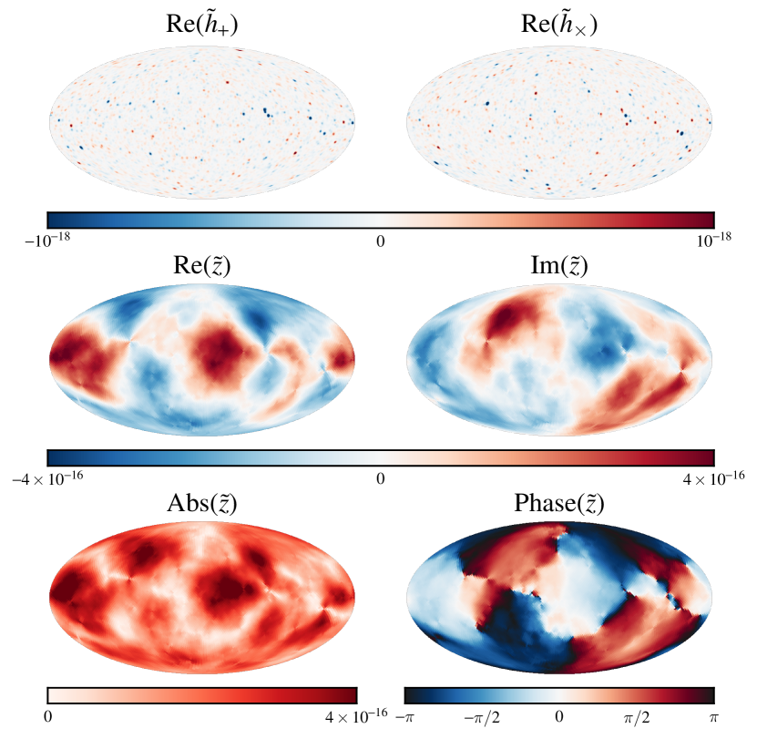
Figure 2: A gwb produced by a population of smbbhs in a frequency bin with a central value of $10$ nHz and a width of $1/10$ yr. The first row shows the real components of $\tilde{h}_{+}$ and $\tilde{h}_{\times}$ produced at the source locations, smoothed to $2^{\circ}$ and clipped at an amplitude of $10^{-18}$ to show detail (maxima are $\sim 10^{-16}$). The imaginary components, not pictured, are similar. Other rows show the induced redshift map. The middle row shows the real and imaginary components, and the bottom row shows the same map in terms of amplitude and phase. The $\tilde{z}$ maps show that the background has some source confusion, but a handful of the brightest sources contribute most of the signal.

As this gravitational wave (assumed to originate far outside our galaxy) passes a pulsar and the earth, the pulse train seen on earth gains a frequency shift of

$$\frac{\Delta\nu}{\nu}=z(t,\hat{p},\hat{k})=\frac{1}{2}\frac{p^{i}p^{j}}{1+\hat{k}\cdot\hat{p}}\big{[}h_{ij}(t_{\text{psr}},\hat{k})-h_{ij}(t_{\text{earth}},\hat{k})\big{]},$$ (10)

where the direction to the pulsar is written $\hat{p}$. Frequency shifts will be of the same order of magnitude as $h$, that is $\lesssim 10^{-15}$. This is too small to measure. However, over many cycles, the frequency shift will affect the time of arrival of the pulses:

$$r(t,\hat{p})=\int_{0}^{t}dt^{\prime}z(t^{\prime},\hat{p}),$$ (11)

producing the gw contribution to pta timing residuals. The amplitude of $r$ will be of order $h/f\lesssim 100$ ns for waves with $f\sim 10$ nHz.

Since the gws will pass through our entire galaxy, $z(t,\hat{p})$ (and equivalently, $r$) can be split into two terms: the term due to the metric disturbance at the earth, $h_{ij}(t_{\text{earth}},\hat{k})$, and the term at the pulsar. Earth terms due to the same gw will be correlated between different points on the sky (different pulsars), but pulsar terms will depend on the distance between the earth and the pulsar. Absent detailed information about pulsar distances, and assuming that the sources do not evolve significantly in frequency between the time that the waves pass the earth and all pulsars, pulsar terms can be modeled as a term of the same magnitude as the earth term but with a random additional phase. For simplicity, the rest of the paper will concentrate on the earth terms, which are correlated on the sky, although they can also be considered as a form of self-noise, which would enter the calculations in Section 5.

Assuming circular binaries, we write

$$\tilde{z}_{\text{earth}}(f,\hat{p},\hat{k})=\frac{1}{2}\frac{p^{i}p^{j}}{1+\hat{k}\cdot\hat{p}}\tilde{h}_{ij}(f,\hat{k}),$$ (12)

where $\tilde{h}_{ij}(f,\hat{k})$ is of the form given in Equation 9. This is a complex scalar field. Calculating the total redshift induced in any one direction $\hat{p}$ requires integration over all $h_{ij}$ coming from all directions $\hat{k}$.

We present two examples of $\tilde{z}_{\text{earth}}$ in a single frequency bin. Figure 1 shows the redshift map produced by two smbbh sources of the same amplitude but different inclinations and random other parameters. Figure 2 is an example of a likely gwb for a single frequency bin. It is generated from the population models of Roebber et al. (2016). Every binary black hole is assigned a random set of parameters. Although the population contains 150,000 gw sources with $\mathcal{M}>10^{7}M_{\odot}$, relatively few are visible in the maps.

3 Harmonic analysis of redshift maps

We consider two toy model gwbs which can be considered as limiting cases for a stochastic gwb produced by a population of smbbhs with no underlying anisotropy. The first example is for a single source of gws, which is an idealization of the case where the gw power in a frequency bin is dominated by a single bright source. The second example is the canonical case where the gwb is a stochastic Gaussian random field. This represents the opposite limit of a confusion background, which has no visible individual sources.

3.1 A single gravitational wave source

For the case of a single source, we will consider a single inspiraling pair of smbbhs located at the north pole and aligned with our $(l,m)$ coordinate choices, so that $\psi=0$ and $\phi=0$. This choice will allow us to do the calculations in a simple form; all other possible single sources can be reproduced by applying a rotation at the end.

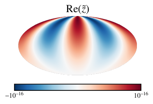
Figure 3: The redshift pattern produced for an edge-on single source at the north pole with gw amplitude $\mathcal{A}=10^{-16}$ and $\psi=0$. For this example, there is no imaginary component. The integrated redshift term which affects the pulsar timing residuals looks very similar, but has a maximum amplitude of $\mathcal{A}/2\pi if$, rather than $\mathcal{A}$.

In this coordinate system, the direction of the gw propagation is $\hat{k}=-\hat{z}$ and the vectors defining the polarization are $(l,m)=(-\hat{x},\hat{y})$. Plugging these definitions, Equation 3, and Equation 1 into Equation 12 and considering the response in all directions $\hat{r}=(\theta,\phi)$ produces the redshift induced across the sky by a single source at the north pole:

$$\tilde{z}(\theta,\phi)=\frac{1}{2}(1+\cos\theta)(\cos 2\phi\,\tilde{h}_{+}-\sin 2\phi\,\tilde{h}_{\times}).$$ (13)

This is a continuous field everywhere except in the direction of the source, where the $\theta$ term is constant, but the $\phi$ term is undefined due to rapid oscillation at small $\theta$. See Figure 3.

Since Equation 13 is a scalar field, it can be represented as the sum of spherical harmonics. Doing this expansion (see Appendix A) produces

$$a_{lm}=2\pi\sqrt{\frac{2l+1}{4\pi}\frac{(l-2)!}{(l+2)!}}(\tilde{h}_{+}\pm i\tilde{h}_{\times}),\text{ for }m=\pm 2.$$ (14)

Note that the subscripts $l,m$ here are the usual spherical harmonic labels and not tensor indices. Interestingly, the $a_{lm}$ only exist for $m\pm 2$. This is a reflection of the four stripes seen in the half-beachball form of the pulsar response function (see Figure 3). Fundamentally, this is due to the spin-2 nature of gravitational waves—a rotation of the $(\hat{l},\hat{m})$ coordinate system by $180^{\circ}$ must produce the same result.

Although the underlying form of the redshift pattern is fundamental, the representation in spherical harmonics is a result of our choice to place the gw source at the north pole. A source located elsewhere in the sky can be expressed by a rotation of Equation 14. This will mix between $m$ components, so that a generic source will require a full set of spherical harmonics to reproduce its response function. However, since rotations of spherical harmonics cannot transform one $l$ to another, the scaling of $a_{lm}$ with $l$ will remain consistent.

A statistical description of the $l$-scaling of $z$ can be found in the angular power spectrum (Dodelson, 2003):

$$C_{l}=\frac{1}{2l+1}\sum_{m}a_{lm}^{*}a_{lm}$$ (15)

For the case of a single source, this becomes:

$$C_{l}=\frac{2\pi\left(\tilde{h}_{+}^{2}+\tilde{h}_{\times}^{2}\right)}{(l+2)(l+1)(l)(l-1)},\text{ for }l\geq 2.$$ (16)

This is a steeply decreasing function of $l$. Since it is only a function of $l$ it does not vary under rotations. Therefore, Equation 16 holds for any single smbbh source of gws with polarizations $\tilde{h}_{+}$ and $\tilde{h}_{\times}$.

3.2 A statistically isotropic Gaussian random field gravitational wave background

The second case that we consider is the case where the gwb is a statistically isotropic Gaussian random field. This represents an idealization of a stochastic background produced by many sources, and similar models have frequently been considered in the pta literature. Our discussion will follow Burke (1975).

This kind of background is the most similar to the cmb. However, a major difference is that the gwb is stationary but not time-invariant on observational timescales. (This is because it is produced by rotating smbbhs, which cause the background to rotate through polarizations). When we Fourier transform the data to work with a single frequency bin, the resulting maps will be complex, unlike the real cmb maps.

A gwb produced by smbbhs produces a redshift field equal to the sum over the redshift field produced by each source. Every source will produce a redshift field of the form of Equation 13, but with an additional random rotation, which sets $(\theta,\phi,\psi)$ to random new values. For a field with maximal source confusion, we consider independent sources of similar amplitude along every line of sight.

As we incoherently add sources, the value of each of the $a_{lm}$’s will change. However, since the $l$-dependence is left unchanged after a rotation, the new $a_{lm}$’s will be given by a sum of terms with varying complex amplitude, but which all scale with $l$ in the same way as Equation 14. In this way we can see that adding sources preserves the shape of the average power spectrum. An example is shown in Figure 4.

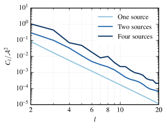
Figure 4: The power spectrum for $z$ maps containing several random sources with amplitude $\mathcal{A}$. One source produces a power spectrum that scales exactly as $[(l+2)(l+1)(l)(l-1)]^{-1}$. Adding a second source has two effects: increasing the amplitude and inducing small interference ripples around the fiducial power law. Adding more sources to the map will continually increase the amplitude and change the ripples, but they will remain a secondary effect.

The amplitude of the average power spectrum is however strongly affected by the number (and strength) of gw sources. For fixed $l$, adding randomly-located sources can be modeled as a random walk in the amplitudes of each mode. The random walk will have a mean of zero, but the variance will increase proportionally to the number of sources. Since the power spectrum is the variance of the $a_{lm}$, a Gaussian random field produced by $N_{\text{src}}$ identical sources should have an underlying power spectrum of the form:

$$C_{l}\propto\frac{N_{\text{src}}}{(l+2)(l+1)(l)(l-1)}.$$ (17)

In other words, adding many sources of similar amplitude randomly and incoherently will produce a field whose harmonic decomposition is made up of terms arbitrarily drawn from a distribution given by Equation 17. In real space, this means that as the number of sources increase, points separated by given angle will maintain an average correlation, but actual values will be randomly distributed according to a Gaussian distribution.

A fully Gaussian random field is shown in Figure 5. By comparing Figure 5 and the low-frequency population model gwb shown in Figure 2, we see that the population produces a mostly-Gaussian field, but with small artifacts around the brightest sources. While the distribution of source amplitudes in a real population is steeply decreasing, it is still true that a relatively small number of sources produce a majority of the signal.

It is important to recall that while Equation 17 gives the expectation value for the power spectrum of the field, any single realization will only approximately reproduce it. We will discuss this further in Section 4.3.

Figure 5: A single realization of a statistically-isotropic gaussian random redshift map with a power spectrum given by Equation 17.

4 Variance in the power spectrum and the Hellings & Downs curve

In this section we will discuss the relationship between the power spectrum of the redshift map and the Hellings & Downs curve. We will explore how variance around the fiducial power law power spectrum affects the shape of the two-point correlation function in the gwb models previously discussed. Since redshifts may be readily converted into timing residuals independently of angle, the following analysis applies to both.

4.1 The power spectrum is the harmonic transform of the Hellings & Downs curve

In the standard pta analysis, timing residuals from different pulsars are correlated. This process should average away effects of noise, which is expected to be uncorrelated between different pulsars (e.g. Lommen, 2015). Correlations due to passing gws in the timing residuals of two pulsars separated by an angle $\theta$ are expected to take the form of the Hellings & Downs curve (Hellings & Downs, 1983):

$$C(\theta)=\frac{1}{2}\left\{1+\frac{3}{2}(1-\cos\theta)\left[\ln\left(\frac{1-\cos\theta}{2}\right)-\frac{1}{6}\right]\right\}.$$ (18)

This is a real-space two-point correlation function (also sometimes referred to as an overlap reduction function). It is an especially useful statistic for a Gaussian random field, since the statistics of such a field can be described entirely by the mean (one-point function) and standard deviation (two-point function), e.g. Allen & Romano (1999). For symmetric fields such as the gwb or the cosmic microwave background, the mean vanishes, ensuring that the two-point function contains the entire statistical information of the field.

If we consider taking the two-point function of a large number of points across the sky (e.g. the pixels in a map such as those shown in Figure 1), it becomes sensible to define a harmonic-space analog of the two point correlation function. This function is the power spectrum discussed earlier, and the conversion between the two forms may be written (Dodelson, 2003):

$$C(\theta)=\sum_{l=0}^{\infty}C_{l}\frac{2l+1}{4\pi}P_{l}(\cos\theta),$$ (19)

where $C_{l}$ is given Equation 17.

A proof for this relation is shown in Gair et al. (2014), although they use different notation: their $C_{l}$ is a constant since they are concerned with the power spectrum of the gw point source distribution. Their additional factor of $N_{l}^{2}$ is equivalent to the $l$-scaling in our choice of $C_{l}$, and represents the effect of the pulsar response function.

An additional concern is the normalization of Equation 17 required to reproduce the standard form of the Hellings & Downs relation. This can be found from Equation 19, as done by Gair et al. (2014), or by considering Parseval’s theorem for spherical harmonics:

$$\sum_{l=0}^{\infty}\sum_{m=-l}^{l}|a_{lm}|^{2} =\int_{S^{2}}d\Omega\,|\tilde{z}(\theta,\phi)|^{2}$$

$$\sum_{l=2}^{\infty}(2l+1)C_{l} =4\pi\,C(0).$$ (20)

Doing the sum produces a factor of $1/3$, so the normalization of the power spectrum required to satisfy this constraint is

$$C_{l}=\frac{6\pi}{(l+2)(l+1)(l)(l-1)}.$$ (21)

Since the Hellings & Downs curve is the map space version of the expected form of the angular power spectrum, any effects which modify the power spectrum can be converted into potentially measurable effects on the two-point correlation function.

4.2 Variance in the Hellings & Downs curve for a single gravitational wave source

For a single source of gravitational waves at the north pole, we were able to calculate the $a_{lm}$ exactly (up to a rotation). The only uncertainty left is in the amplitudes of the two polarizations, which will be specified by the value of the parameters $\mathcal{A},\Phi_{0},\iota,\psi$ for any single source. Since there is no uncertainty in the underlying $a_{lm}$, the form of the $C_{l}$ is given by Equation 16, with no variance. This will produce a real-space two-point correlation that is exactly equivalent to the Hellings & Downs curve.

If we add a second source to the map, the form of the $a_{lm}$ gains additional degrees of freedom relating to the angle between the two sources and their relative orientations. In general, the two redshift patterns will interfere, leading to maps like those in Figure 1 and power spectra similar to Figure 4. The primary effect on the power spectrum is to roughly double its amplitude (depending on parameter values). The ripples induced by the interference are typically a smaller effect.

As a result, the primary effect on the two-point correlation is to increase the signal. The small ripples will result in a mild change in the shape of the correlation function away from Hellings & Downs. This will be discussed in greater detail in the next section.

When the two sources are appropriately aligned, more dramatic effects can be produced. Co-located sources with out-of phase redshift patterns can cancel, and sources separated by $90^{\circ}$ can have power spectrum oscillations of $20$–$50\%$ at low $l$. In these cases, the two-point correlation will either have decreased signal (as in the first case) or the shape will change significantly (the second case).

4.3 Variance in the Hellings & Downs curve for a Gaussian random field

For a statistically isotropic Gaussian random gravitational wave field, the expectation value of the power spectrum will be of the form of Equation 17. However, we are able to observe only one realization of the gwb.

For a Gaussian random background, all multipole moments $a_{lm}$ are drawn from a Gaussian distribution with variance $C_{l}$. Even if we are able to measure the $a_{lm}$ perfectly, our ability to correctly estimate the variance of the distribution will be affected by the number of modes for each value of $l$. Therefore, the observed power spectrum $\hat{C}_{l}$ will not be of the same form as the expectation value $C_{l}$.

In contrast, for a single source, the choice of each $a_{lm}$ depends on the sky location and polarization angle of the source, but is otherwise entirely set. The distribution is entirely random for a Gaussian field, and entirely non-random for a single source.

This limitation on the measurability of $C_{l}$ is the cosmic variance familiar from calculations of the cosmic microwave background power spectrum:

$$\Delta C_{l}=\frac{C_{l}}{\sqrt{2l+1}}.$$ (22)

This equation differs from the standard definition (e.g. Dodelson, 2003) by a factor of $\sqrt{2}$. Since the Fourier-transformed gwb is a complex field, it contains twice the information of a real field such as the cmb.

The cosmic variance represents the range within which an observed $\hat{C}_{l}$ is expected to differ from the true unobservable $C_{l}$ for each $l$. When $\hat{C}_{l}$ no longer follows Equation 17, $\hat{C}(\theta)$ will no longer follow the Hellings & Downs curve. By changing a single multipole, we are effectively changing the weights of individual Legendre polynomials in Equation 19.

Since $C_{l}$, and consequently $\Delta C_{l}$, is a strong function of $l$, the effect of cosmic variance will be strongest for the first few multipoles. This is shown in Figure 6. The quadrupole term is by far the most important, but combinations of several other terms can also affect the shape of the two-point correlation function.

Figure 6: The effect on the Hellings & Downs curve due to changing a single term of the power spectrum by an amount within the cosmic variance. The solid dark line is the Hellings & Downs curve and the edges of the shaded region marked with $+$ or $-$ respectively represent the effects of increasing or decreasing the power spectrum term.

It will often be the case that the power spectrum of a Gaussian random gwb will have a low or high quadrupole or octopole by chance. It would therefore not be surprising to have a two-point correlation function which does not match the Hellings & Downs curve. Note that in contrast to the work in Mingarelli et al. (2013); Taylor & Gair (2013); Gair et al. (2014), this change in shape of the two-point correlation function is not due to large-scale anisotropy in the source population, but occurs even in statistically-isotropic gwbs.

For two sources which induce a noticeable shape shift on the two point correlation function, the basic mechanism is the same as for the Gaussian case: specific Legendre polynomials in the expansion of Equation 19 are being up- or downweighted. The primary difference in these two cases is that for a Gaussian field, the amount by which each $C_{l}$ varies from the expectation value is independent of all the others. For two sources, the specific interference pattern between the two redshift maps leads to oscillations in the power spectrum. These oscillations are set by the relative orientation and distance of the sources and are not random and not independent.

So far we have been discussing a gwb composed of a single frequency bin. However, ptas are typically sensitive to a range of frequencies. If all the frequency bins under consideration can be described by the same underlying distribution, the effect of cosmic variance can be ameliorated. This is because the separate frequency bins can be considered as independent realizations of the same map—including more frequency bins allows us to sample the distributions more accurately. From Equation 22, $\Delta C_{l}\sim(N_{\text{modes}})^{-1/2},$ so using $n$ similar bins in the analysis will reduce the cosmic variance by a factor of $\sqrt{n}$. Even for a single frequency bin, an analysis assuming Hellings & Downs behavior may be sufficient to allow an initial detection (Cornish & Sampson, 2016).

5 How well can a pta measure the angular power spectrum?

Our analysis has focused on the analysis of redshift maps in harmonic space, inspired by cmb analyses. However, unlike cmb experiments which make measurements over large regions of the sky, ptas are only sensitive to the redshift field in the direction of its pulsars. The observed field is a partial sky map, sampled at $M$ discrete sky locations corresponding to the positions of the pulsars in the array.

The number of pulsars will limit the degree to which a pta can measure harmonics of the gwb, but the steepness of the power spectrum will turn out to be a more important limitation. We estimate pta sensitivity to the power spectrum through the following signal-to-noise calculation.

For a sparse sampling of the sky, an estimate of a spherical harmonic expansion of a field $r(\theta,\phi)$ sampled at points $(\theta_{i},\phi_{i})$ can be constructed as

$$\hat{a}_{lm}=\frac{4\pi}{\sum_{i}w_{i}}\sum_{i}w_{i}Y_{lm}(\theta_{i},\phi_{i})r(\theta_{i},\phi_{i}),$$ (23)

where $w_{i}$ are weights that can be tuned for each point. The minimum variance estimate will have $w_{i}$ equal to $1/\sigma_{i}^{2}$, where $\sigma_{i}$ is the variance at each point. The formally optimal solution would have $\sigma_{i}$ only including detector noise and terms intrinsic to the pulsar. However, in practice it would be difficult to separate a given pulsar’s noise properties from a gravitational wave background.

For simplicity, we assume that all pulsars have equal weight, with rms noise of each pulsar (for gravitational waves plus noise) $\sigma_{0}$. Generalizing to varying noise levels is straightforward. For $M$ pulsars, the estimated angular power spectrum will then have a noise bias:

$$C_{l}^{N}=\frac{4\pi}{M}\sigma_{0}^{2}\ .$$ (24)

We can use Equation 22 to estimate the signal to noise of the amplitude for a pta, taking care to realize that the relevant $C_{\ell}$ for the noise estimate is the combined signal and noise power spectrum. For the signal power spectrum, we know that the form should follow from Equation 21. Given a variance in residuals from gravitational waves $\sigma_{gw}^{2}$, we write

$$C_{l}^{S}=\sigma_{gw}^{2}C_{l}.$$ (25)

The resulting estimate for the signal to noise for a given multipole $l$ is

$$\left(\frac{S}{N}\right)_{l}^{2}=(C_{l}^{S})^{2}\frac{2l+1}{(C_{l}^{S}+C_{l}^{N})^{2}}$$ (26)

For a first detection, the expectation is that the noise power in the large-scale correlated timing residuals will be much larger than the signal power. We can then simplify the signal-to-noise estimate by dropping the signal part of the last term. Explicitly, the signal-to-noise in the limit of a weak detection is

$$\left(\frac{S}{N}\right)_{l;\text{ weak}}^{2}=\frac{9}{4}\frac{2l+1}{[(l-1)l(l+1)(l+2)]^{2}}\frac{M^{2}\sigma_{gw}^{4}}{\sigma_{0}^{4}}$$ (27)

Summing this over all $\ell$ gives a numerical prefactor of $1/48$, with the $l=2$ term alone contributing $5/256$. The $l=2$ term thus contributes 93.75% of the $(S/N)^{2}$. If one only measured the power in the quadrupole anisotropy of the timing residuals, the resulting signal-to-noise would be 97% of the total signal-to-noise available. This is simply because the quadrupole is contributing such a large fraction of the total power that it is far and away the largest signal to be measured and the signal-to-noise adds in quadrature rather than linearly.

To compare with previous work, we can do the similar calculation in map space. As shown in Siemens et al. (2013), the comparable prefactor for this calculation in map space reduces to the total number of pairs times the mean of the square of the Hellings & Downs curve. For a full-sky survey, the mean of the square of the Hellings & Downs curve is 1/48, while the number of unique pulsar pairs is $M(M-1)/2$, very close to $M^{2}/2$, with the $(M-1)$ instead of $M$ coming from the explicit nulling of autocorrelations in the calculation.

6 Discussion

In this work we have introduced an alternate framework for considering spatial variation in gravitational wave backgrounds. We primarily work with the all-sky redshift patterns induced by gravitational waves passing the earth. Using standard techniques from cmb analysis, we do all calculations in harmonic space for computational simplicity, but convert to map space to discuss measurable quantities. Since we assume non-evolving gw sources, all results are also true for the earth term of the expected pulsar timing residuals, up to a normalization. This assumption breaks down for rare high-mass, high-frequency binaries which evolve on timescales of $\sim$ kyr rather than $\sim$ Myr (Mingarelli et al., 2012).

We explicitly decomposed the redshift pattern produced by a single source of gws into spherical harmonics, which allowed us to calculate the power spectrum of a single source’s redshift map exactly. We showed that the expectation value of the power spectrum for a statistically isotropic gaussian random gwb has the same form as for a single source. Using the relation between the power spectrum and the real space two-point correlation function, we explored the degree to which variance in the power spectrum changes the shape of the two-point correlation function away from Hellings & Downs. In particular, cosmic variance in the quadrupole moment of the power spectrum for a Gaussian random field can have significant effects on the amplitude of the curve, while also changing its shape. Finally, we showed that the quadrupole term of the power spectrum contributes $97\%$ of the signal-to-noise measured by a pta.

Throughout this work, we have treated the gwb as one of two idealized cases: a single source or a Gaussian random field. A gwb produced by a population of sources will lie somewhere between these two cases, as suggested by Figure 2. It is likely that the degree to which a population of sources resembles one case or another changes as a function of frequency, with shot noise in the smbbh population becoming more important at higher frequencies.

We have confirmed that gwbs dominated by a single bright source, which are highly anisotropic and non-Gaussian, and those which are isotropic, unpolarized, and Gaussian look very similar from the point of view of a two-point correlation function, as previously reported by Cornish & Sesana (2013). This suggests that two-point correlation functions will be effective for detecting gwbs of all kinds. But they will be ineffective for characterizing gwbs and searching for single sources, despite the clear visual differences between Figure 3 and Figure 5.

This difference should be measurable given a sufficiently high significance measurement of the gwb and some luck in its orientation with respect to low-noise pulsars. A particularly clear example is given in Boyle & Pen (2012): consider the timing residuals for four pulsars, each of which is located in a different stripe near the top of the map in Figure 3. The gw signal in each pulsar will be perfectly correlated, differing only by a phase factor of $180^{\circ}$ between adjacent stripes. No such perfect (anti-)correlation is possible for nearby pulsars affected by a Gaussian field such as in Figure 5.

An important difference between these two types of gwbs is that the redshift map produced by a single source is highly nongaussian. Although symmetric Gaussian distributions can be statistically completely described by their two-point functions, non-Gaussian distributions may have higher moments. Indeed, the example given by Boyle & Pen (2012) is a kind of four-point function. Future work will explore higher-order correlation functions as a means of characterizing the degree to which a gwb has Gaussian or point-source-like characteristics.

Appendix A Calculating the harmonic expansion of $\tilde{z}(\theta,\phi)$ for a single source GWB

From Equation 13, we have the redshift induced in a direction $(\theta,\phi)$ by a source located at the north pole. This is a complex scalar field, and can be expanded in spherical harmonics with coefficients:

$$a_{lm} =\int d\Omega\,\left[\frac{1}{2}(1+\cos\theta)(\cos 2\phi\,h_{+}-\sin 2\phi\,h_{\times})\right]Y_{lm}^{*}$$ (A1)

$$=\underbrace{\frac{1}{2}(-1)^{m}\sqrt{\frac{2l+1}{4\pi}\frac{(l-m)!}{(l+m)!}}}_{\text{A}}\;\overbrace{\int_{0}^{2\pi}d\phi\,e^{-im\phi}\left(\cos 2\phi\,\tilde{h}_{+}-\sin 2\phi\,\tilde{h}_{\times}\right)}^{\text{B}}\;\underbrace{\int_{0}^{\pi}d\theta\,\sin\theta\,(1+\cos\theta)P_{l}^{m}(\cos\theta)}_{\text{C}},$$ (A2)

where $P_{l}^{m}(\cos\theta)$ are the associated Legendre polynomials. This factorizes into two integrals ($B$, $C$) and one constant term ($A$). Beginning with the integral over $\phi$, we find that it simplifies to

$$B=\frac{1}{2}\left(\tilde{h}_{+}+i\tilde{h}_{\times}\right)\int_{0}^{2\pi}d\phi\,e^{-i\phi(m-2)}+\frac{1}{2}\left(\tilde{h}_{+}-i\tilde{h}_{\times}\right)\int_{0}^{2\pi}d\phi\,e^{-i\phi(m+2)}.$$ (A3)

Since $\int_{0}^{2\pi}d\phi\,\exp(-\alpha i\phi)=2\pi\,\delta(\alpha)$ for real $\alpha$, only terms with $m=\pm 2$ exist. They are given by

$$B=\begin{cases}\pi(\tilde{h}_{+}\pm i\tilde{h}_{\times}),&m=\pm 2\\ 0,&\text{all other $m$}\end{cases}.$$ (A4)

This constraint on $m$ allows us to simplify both our constant term and $\theta$ integral:

$$A\cdot C =\frac{1}{2}\sqrt{\frac{2l+1}{4\pi}\frac{(l\mp 2)!}{(l\pm 2)!}}\int_{0}^{\pi}d\theta\,\sin\theta(1+\cos\theta)P_{l}^{\pm 2}(\cos\theta)$$ (A5)

$$=\frac{1}{2}\sqrt{\frac{2l+1}{4\pi}\frac{(l-2)!}{(l+2)!}}\int_{0}^{\pi}d\theta\,\sin\theta(1+\cos\theta)P_{l}^{2}(\cos\theta),$$ (A6)

using the following property of associated Legendre polynomials:

$$P_{l}^{-m}=(-1)^{m}\frac{(l-m)!}{(l+m)!}P_{l}^{m}.$$ (A8)

Writing $\mu=\cos\theta$, we solve the integral over $\theta$:

$$C =\int_{-1}^{1}d\mu\,(1+\mu)P_{l}^{2}(\mu)$$ (A9)

$$=\int_{-1}^{1}d\mu\,(1+\mu)(1-\mu^{2})\frac{d^{2}}{d\mu^{2}}P_{l}(\mu)$$ (in terms of ordinary Legendre polynomials) (A10)

$$=\int_{-1}^{1}d\mu\,(1+\mu)\left[2\mu\frac{d}{d\mu}P_{l}(\mu)-l(l+1)P_{l}(\mu)\right]$$ (using the defining differential equation) (A11)

$$=\int_{-1}^{1}d\mu\,(1+\mu)2\mu\frac{d}{d\mu}P_{l}(\mu)$$ (second term zero by orthogonality) (A12)

$$=\left[2\mu^{2}P_{l}(\mu)+2\mu P_{l}(\mu)\right]_{-1}^{1}-\int_{-1}^{1}d\mu\,(4\mu+2)P_{l}(\mu)$$ (A13)

$$=2\left[P_{l}(1)+P_{l}(1)+P_{l}(-1)-P_{l}(-1)\right]$$ (second term zero by orthogonality) (A14)

$$=4$$ (A15)

Putting everything together,

$$a_{lm}=A\cdot B\cdot C=\begin{dcases}2\pi\sqrt{\frac{2l+1}{4\pi}\frac{(l-2)!}{(l+2)!}}\big{(}\tilde{h}_{+}\pm i\tilde{h}_{\times}\big{)},&m=\pm 2,\,l\geq 2.\\ 0,&\text{otherwise.}\end{dcases}$$ (A16)

References

- Abbott et al. (2016) Abbott, B. P., Abbott, R., Abbott, T. D., et al. 2016, PRL, 116, 131103
- Allen & Romano (1999) Allen, B., & Romano, J. D. 1999, Phys. Rev. D, 59, 102001
- Arzoumanian et al. (2016) Arzoumanian, Z., Brazier, A., Burke-Spolaor, S., et al. 2016, ApJ, 821, 13
- Babak & Sesana (2012) Babak, S., & Sesana, A. 2012, Phys. Rev. D, 85, 044034
- Boyle & Pen (2012) Boyle, L., & Pen, U.-L. 2012, Phys. Rev. D, 86, 124028
- Burke (1975) Burke, W. L. 1975, ApJ, 196, 329
- Corbin & Cornish (2010) Corbin, V., & Cornish, N. J. 2010, arXiv:1008.1782
- Cornish & Sampson (2016) Cornish, N. J., & Sampson, L. 2016, Phys. Rev. D, 93, 104047
- Cornish & Sesana (2013) Cornish, N. J., & Sesana, A. 2013, CQGra, 30, 224005
- Cornish & van Haasteren (2014) Cornish, N. J., & van Haasteren, R. 2014, arXiv:1406.4511
- Cutler & Flanagan (1994) Cutler, C., & Flanagan, É. E. 1994, Phys. Rev. D, 49, 2658
- Dodelson (2003) Dodelson, S. 2003, Modern cosmology (Academic Press)
- eLISA Consortium (2013) eLISA Consortium. 2013, arXiv:1305.5720
- Foster & Backer (1990) Foster, R. S., & Backer, D. C. 1990, ApJ, 361, 300
- Gair et al. (2014) Gair, J., Romano, J. D., Taylor, S., & Mingarelli, C. M. F. 2014, Phys. Rev. D, 90, 082001
- Górski et al. (2005) Górski, K. M., Hivon, E., Banday, A. J., et al. 2005, ApJ, 622, 759
- Hellings & Downs (1983) Hellings, R. W., & Downs, G. S. 1983, ApJ, 265, L39
- Hunter (2007) Hunter, J. D. 2007, Computing In Science & Engineering, 9, 90
- Kocsis & Sesana (2011) Kocsis, B., & Sesana, A. 2011, MNRAS, 411, 1467
- Lentati et al. (2015) Lentati, L., Taylor, S. R., Mingarelli, C. M. F., et al. 2015, MNRAS, 453, 2576
- Lommen (2015) Lommen, A. N. 2015, Rep. Prog. Phys., 78, 124901
- Maggiore (2008) Maggiore, M. 2008, Gravitational Waves, Vol. 1 (Oxford University Press)
- Mingarelli et al. (2012) Mingarelli, C. M. F., Grover, K., Sidery, T., Smith, R. J. E., & Vecchio, A. 2012, PRL, 109, 081104
- Mingarelli et al. (2013) Mingarelli, C. M. F., Sidery, T., Mandel, I., & Vecchio, A. 2013, Phys. Rev. D, 88, 062005
- Ravi et al. (2012) Ravi, V., Wyithe, J. S. B., Hobbs, G., et al. 2012, ApJ, 761, 84
- Roebber et al. (2016) Roebber, E., Holder, G., Holz, D. E., & Warren, M. 2016, ApJ, 819, 163
- Rosado et al. (2015) Rosado, P. A., Sesana, A., & Gair, J. 2015, MNRAS, 451, 2417
- Sesana & Vecchio (2010) Sesana, A., & Vecchio, A. 2010, Phys. Rev. D, 81, 104008
- Sesana et al. (2008) Sesana, A., Vecchio, A., & Colacino, C. N. 2008, MNRAS, 390, 192
- Shannon et al. (2015) Shannon, R. M., Ravi, V., Lentati, L. T., et al. 2015, Science, 349, 1522
- Siemens et al. (2013) Siemens, X., Ellis, J., Jenet, F., & Romano, J. D. 2013, CQGra, 30, 224015
- Simon et al. (2014) Simon, J., Polin, A., Lommen, A., et al. 2014, ApJ, 784, 60
- Taylor & Gair (2013) Taylor, S. R., & Gair, J. R. 2013, Phys. Rev. D, 88, 084001
- Verbiest et al. (2016) Verbiest, J. P. W., Lentati, L., Hobbs, G., et al. 2016, MNRAS, 458, 1267