ASTErIsM - Application of topometric clustering algorithms in automatic galaxy detection and classification

Abstract

We present a study on galaxy detection and shape classification using topometric clustering algorithms. We first use the DBSCAN algorithm to extract, from CCD frames, groups of adjacent pixels with significant fluxes and we then apply the DENCLUE algorithm to separate the contributions of overlapping sources. The DENCLUE separation is based on the localization of pattern of local maxima, through an iterative algorithm which associates each pixel to the closest local maximum.

Our main classification goal is to take apart elliptical from spiral galaxies. We introduce new sets of features derived from the computation of geometrical invariant moments of the pixel group shape and from the statistics of the spatial distribution of the DENCLUE local maxima patterns. Ellipticals are characterized by a single group of local maxima, related to the galaxy core, while spiral galaxies have additional ones related to segments of spiral arms. We use two different supervised ensemble classification algorithms, Random Forest, and Gradient Boosting. Using a sample of $\simeq 24000$ galaxies taken from the Galaxy Zoo 2 main sample with spectroscopic redshifts, and we test our classification against the Galaxy Zoo 2 catalog.

We find that features extracted from our pipeline give on average an accuracy of $\simeq 93\%$, when testing on a test set with a size of $20\%$ of our full data set, with features deriving from the angular distribution of density attractor ranking at the top of the discrimination power.

1 Introduction

Morphology is one of the main characteristics of galaxies, as physical process happening during life time of galaxies strongly determine their shape. Therefore any theory of galaxy formation and evolution needs to closely explain the observational distribution of morphological classes (Dressler, 1980; Bamford et al., 2009; Roberts & Haynes, 1994). Accurate information of galaxy types gives insight also well beyond galaxy research, testing cosmological models by studying large scale structure with ETG clustering (Naab et al., 2007), dark mater probe by strong gravitational lensing (Koopmans, 2004; Treu & Koopmans, 2002)

The key challenge of all this research is accurate and efficient classification of big number of galaxies. Traditional method of morphological classification classifies galaxies according to Hubble’s scheme (Sandage, 1961). This system classifies the galaxy morphologies into elliptical, lenticular, spiral, and irregular galaxies. However, due to the impressive amount of photometric data produced by large galaxy survey the size and quality modern data sets led to refinements in the classification (Kormendy & Bender, 1996; Cappellari et al., 2011; van der Wel et al., 2007; Kartaltepe et al., 2015)

One possible classification methods is given by citizen science projects. Excellent example of collaborative work on visual galaxy morphology classification is the Galaxy Zoo project that involved more than 100,000 volunteers to determine a galaxy class for about 900,000 (Galaxy Zoo 1) and 304,122(Galaxy Zoo 2) galaxies (Lintott et al., 2011; Willett et al., 2013)

On the other side, larger number of galaxies available in the next generation of all-sky survey missions (Euclid, LSST, KIDS etc) makes such a human-eye analysis unmanageable. Thus, to classify large numbers of galaxies into early and late types it is compelling to use instead automated morphological classification methods.

Several methods have been used to tackle this challenge, i.e. neural networks (Naim et al., 1995; Lahav et al., 1996; Goderya & Lolling, 2002; Banerji et al., 2010; Dieleman et al., 2015) , decision trees (Owens et al., 1996) and ensembles of classifiers (Bazell & Aha, 2001).

However, because visual inspection requires significant spatial resolution, it is limited in galaxy sample size and it is burden with possibility of missing rare and interesting objects due to lack of scientific knowledge of volunteers. Moreover, significantly larger number of galaxies available in the next generation of all-sky survey missions (Euclid, LSST, KIDS etc) makes such a human-eye analysis unfeasible.

In this paper we present an automated approach, based on a novel combination of two topometric clustering algorithms: the DBSCAN (Ester et al., 1996), and the DENCLUE (Hinneburg & Keim, 1998; Hinneburg & Gabriel, 2007). The DBSCAN algorithm has been already successfully applied to the detection of sources in $\gamma-$ray photons lists (Tramacere & Vecchio, 2013; Carlson et al., 2013) and to identify structure in external galaxies (Rudick et al., 2009), while the DENCLUE, to our knowledge, has never been used, so far, in treatment of astronomical images. In particular we have noted that the DENCLUE algorithm, is effective both in the deblending of confused sources, and in the tracking of spiral arms. We have used these algorithms to develop a python package: ASTErIsM ( python AStronomical Tools for clustering-based dEtectIon and Morphometry). This software is used both to detect the sources in CCD images, and to extract features relevant to the morphological classification.

Figure 1: Flow chart diagram for the detection process.

The paper is organized as follows: In Sec. 2, we describe the detection process, and in particular how we modified DBSCAN and DENCLUE algorithms to work on CCD images. In Sec. 3, we describe how the DENCLUE method can be used to track spiral arms. In Sec. 4 we present a general view of the ASTErIsM pipeline for automatic detection and morphological classification, the sample used in our paper, the feature extractions process, and their statistical characterization. In Sec. 5 we describe the setup of the training sets. In Sec. 6 we describe the algorithms used for our supervised classification (Random Forest (Breiman, 2003) and Gradient Boosting (Friedman, 2001)), and the metrics used for the classification. In Sec. 7 we describe the strategy of our machine learning classification pipeline, and in Sec. 8 we present the results of the classification together with a comparison to other similar works. In Sec. 9, we present our final conclusions and future developments. The code will be available at https://github.com/andreatramacere/asterism

Figure 2: Application of the DBSCAN algorithm to source detection (see Sec. 2.1). The input image is a gri summed bands image cutout centered on the object with DR8OBJID=1237667549806657543 from the Galaxy Zoo 2 Main sample with spectroscopic redshifts. Left panel: the original image. Central panel: pixels selected (white dots), with flux values above the background threshold. Right panel: the tow sources detected by the DBSCAN algorithm, with $N_{bkg}=3.9$, $K=1.5$ and $\varepsilon=1.0$. The withe line shows the source contour, the black crosses show the source centroid, and the yellow ellipses represent the containment ellipsoid.

2 Application of density-based clustering methods to detect sources in CCD images

The "density based spatial clustering of applications with noise" algorithm (DBSCAN) (Ester et al., 1996; Zaki & Wagner Meira, 2014), is a topometric density-based clustering method that uses local density of points to find clusters, in data sets that are affected by background noise. Let $N_{\varepsilon}(p_{i})$ be the set of points contained within the N-dimensional sphere of radius $\varepsilon$ centered on $p_{i}$, and $|N_{\varepsilon}(p_{i})|$ the number of contained points, i.e. the estimator of the local density, and $K$ a threshold value. Clusters are built according to the local density around each point $p_{i}$. A point is classified according to the local density defined as:

• core point: if $|N_{\varepsilon}(p_{i})|\geq K$ .

• border point: if $|N_{\varepsilon}(p_{i})|<K$, but at least one core point belongs to $N_{\varepsilon}(p_{i})$.

• noise point, if both the conditions above are not satisfied.

Points are classified according to their inter-connection as:

• directly density reachable: a point $p_{j}$ is defined directly density reachable from a point $p_{k}$, if $p_{j}\in N_{\varepsilon}(p_{k})$ and $p_{k}$ is a core point.

• density reachable: a point $p_{j}$ is defined density reachable from a point $p_{k}$, if exists a chain of directly density reachable points connecting, $p_{j}$ to $p_{k}$.

• density connected: two points $p_{j}$, $p_{k}$ are defined density connected if exits a core point $p_{l}$ such that both $p_{j}$ and $p_{k}$, are density reachable from $p_{l}$.

The DBSCAN builds the cluster by progressively connecting density connected points to each set of core points found in the set. Thanks to its embedded capability to distinguish background noise (even when the background is not uniform), it has been successfully used to detect sources in $\gamma-$ray photon lists (Tramacere & Vecchio, 2013), or to identify structures in N-body simulations of galaxy clusters (Rudick et al., 2009). For a detailed description of the application of the DBSCAN to $\gamma-$ray photon lists, we address the reader to Tramacere & Vecchio (2013). In general, a photon detection event will be characterized by position in detector/sky coordinates, and further possible features (energy, arrival time, etc…). In the case of photon lists (as in $\gamma-$ray astronomy), the detector/sky coordinates of each event can be recorded and the DBSCAN algorithm can be applied to look for density-based clusters, where a cluster is an astronomical source. Events non belonging to any source (clusters), are assigned to background (noise). In the case of CCD images, a DBSCAN suitable representation of the data is less intuitive. Indeed, detected photons are not stored as single events, being integrated and positionally binned in the CCD matrix itself. Since the pixels coordinates have a uniform spatial distribution, we can not use the original estimator of local density $|N_{\varepsilon}(p_{i})|$ to find density based clusters. To overcome this limitation we have modified the DBSCAN algorithm basing on the idea to use the photon counts/flux recorded in each pixel of the CCD as a new estimator of the local density.

2.1 Image segmenation: DBSCAN

In our modified version of the DBSCAN algorithm we have changed the procedure for the estimation of the local density as follows:

• We iterate through each pixel $p_{k,l}$, where $k$ refer to the $k_{th}$ row and $l$ to the $l_{th}$ column of the CCD matrix

• Let $B_{\varepsilon}(k,l)$ be the set of pixels contained in the box centered on the pixel $p_{k,l}$, and enclosing the pixels with columns $k\pm\varepsilon$ and row $l\pm\varepsilon$

• We evaluate the local flux $M_{\varepsilon}(k,l)$ as total flux collected in $B_{\varepsilon}(k,l)$:

  $$M_{\varepsilon}(k,l)=\sum_{(i,j)\in B_{\varepsilon}(k,l)}I(p_{i,j})$$ (1)

The quantity $M_{\varepsilon}(k,l)$ is our estimator for the local density. With this choice the classification in core, border and noise points will read as:

• core point: if $M_{\varepsilon}(k,l)\geq K$ .

• border point: if $M_{\varepsilon}(k,l)<K$, but at least one core point belongs to $B_{\varepsilon}(k,l)$.

• noise point: if both the conditions above are not meet.

The choice to use as DBSCAN scanning brush a box rather than a circle, speeds-up the computational time, indeed we don’t need to evaluate the CCD pixels distances from $p_{k,l}$ , but just to slice the sub-matrix corresponding to $B_{\varepsilon}(k,l)$. We use values of $\varepsilon$ of a few pixels, typically 1. The remaining part of the algorithm, concerning the recursive build-up of the clusters, follows the original implementation.

Figure 3: Distribution of the density attractors (white crosses) for the cluster with ID=0 in central panel of Fig. 4 for different values of $\varepsilon_{d}$ (see Sec. 2.2 ). Lower values of $\varepsilon_{d}$ result in a tighter clustering of the attractors toward the local maxima of the image. The input image is a gri summed bands image cutout centered on the object with DR8OBJID=1237663548511748377 from the Galaxy Zoo 2 Main sample with spectroscopic redshifts.

Figure 4: Application of the DENCLUE algorithm to deblend two confused sources (see Sec. 2.2): original image (left), DBSCAN detection result (center), and result of the detection after DENCLUE-based deblending (right). Source and image provenance are the same as in Fig. 3.

In order to speed-up further the computational time, we have implemented in our version of the algorithm the possibility to remove from the iteration all the CCD pixels with a flux below a given background threshold. The background threshold is evaluated using the following method:

• We split the CCD matrix in N sub-matrices (typically N=10).

• We select the sub-matrix with the lowest integrated flux, and we estimate the mode of the flux distribution $m_{bkg}$, and it’s standard deviation $\sigma_{bkg}$.

• We compute a range of skewness values for distributions obtained by excluding flux values outside $n\sigma_{bkg}$ from the mode, where $n$ range from 0.5 to 2.0 with 0.1 step. We retain the $n$ value which leads to the lowest skewness and call it n*.

• $m_{bkg}$ and $\sigma_{bkg}$ are updated for the new flux distribution sigma-clipped for $n^{*}$

• We set the the pre-filtering background value $bkg_{th}$ at the level of $bkg_{pre-th}=N_{bkg}\sigma_{bkg}+m_{bkg}$ above the mode. The value of $N_{bkg}$ is chosen in the range of $\simeq$ [2.5,3.5], in order to remove the bulk of the background points, but leaving at the same time enough statistic for the noise determination embedded in the DBSCAN.

• We apply a boolean mask to all the CCD pixels with a flux below $bkg_{pre-th}$.

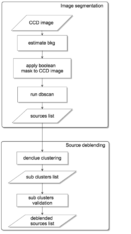
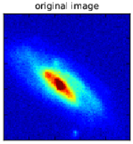
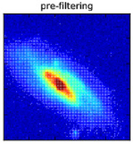
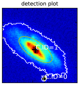
A schematic view of the image segmentation process in shown in the top box of Fig. 1, and an example of the pre-filtering procedure is shown in the left and central panels of Fig. 2. The left pane of Fig. 2. shows the original image, and the white dots in the central panel of the same figure show the pixel selected after the background-based pre-filtering.

The last step, to apply the DBSCAN algorithm, is the setup of the parameters $K$, i.e. the DBSCAN threshold, and $\varepsilon$ i.e. the half width of the DBSCAN scanning box.. The parameter $K$ is the one tuning the DBSCAN internal noise determination, and we use the background pre-filtering to set the value of $K$ using the following method:

• We set $K=K_{th}bkg_{pre-th}$ where the parameter $K_{th}$ is typically in the range of [1.0,2.0].

• To avoid that the value of $K$ depends on $\varepsilon$, $M_{\varepsilon}(p_{k,l})$ is averaged over the number of pixels in the DBSCAN scanning box. In this way the value of $K$ represents a per-pixel threshold.

The second parameter, $\varepsilon$, is the one which tunes the size of the DBSCAN scanning box, hence, low values of $\varepsilon$ will allow to follow accurately also the contour of small objects. For this reason, throughout the present work, we have used $\varepsilon=1.0$ pixels, meaning that the scanning box will have a size of 9 pixels. For each source cluster we evaluate the following relevant parameters:

• $(x_{c},y_{c})$ the centroid coordinates.

• The cluster containment ellipsoid defined by the major and minor semi axis $\sigma_{x},\sigma_{y}$, and by the inclination angle $\alpha_{\rm PCA}$, measured counterclockwise angle w.r.t. the $x$ axis. All these parameters are evaluated by applying the principal component analysis method (PCA) (Jolliffe, 1986), to the covariance matrix of the arrays of the cluster point position $\mathbf{x}$, $\mathbf{y}$, weighted on the cluster pixel flux. This method uses the eigenvalue decomposition of the covariance matrix of the two position arrays $\mathbf{x}$ and $\mathbf{y}$. By definition, the square root of the first eigenvalue will correspond to $\sigma_{x}$, and the second to $\sigma_{y}$.

• $cnt$ the set of the coordinates of the cluster edges pixels

• $r_{pca}=\sqrt{\sigma_{x}^{2}+\sigma_{y}^{2}}$

• $r_{max}$ , i.e. the distance,from the cluster centroid, of the most distant cluster pixel.

The right panel In Fig. 2 shows the final result for an image from our data set, with $N_{bkg}=3.0$, $K_{th}=1.5$ and $\varepsilon=1.0$. The white lines represent the edges pixels of the clusters (sources), and the yellow ellipses represent the cluster containment ellipsoid, defined by $\sigma_{x},\sigma_{y}$, and $\alpha_{\rm PCA}$. The black crosses represent the clusters centroids.

2.2 Source deblending: DENCLUE

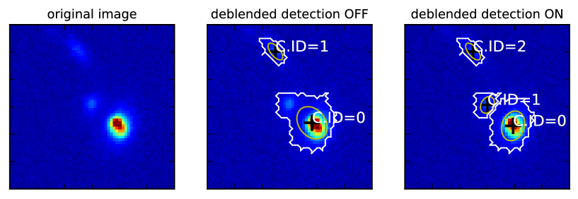
When sources are very close, and/or when we need to use a low value of $K_{th}$ in order to recover faint structures, as in the case of detection of spiral arms, it might happen that the DBSCAN algorithm is not able to separate them (see Fig. 4, central panel).

To deblend two (or more) ‘confused’ sources we have implemented a deblending method based on the DENCLUE algorithm (Hinneburg & Keim, 1998; Hinneburg & Gabriel, 2007; Zaki & Wagner Meira, 2014). The original implementation of the DENCLUE algorithm is based on the kernel density estimation to find local maxima of dense region of points. In the case of digital images it is not possible to apply straightforwardly the equations reported in the original algorithm implementation, indeed the pixels coordinates have a uniform spatial distribution. To overcome this limitation we have modified the DENCLUE algorithm substituting the kernel density estimation with a convolution of the image with a given kernel. Let $p_{j}$ be the $j_{th}$ pixel with coordinates $\mathbf{q_{j}}$, the kernel function $G$ is a non-negative and symmetric function, centered at $\mathbf{q_{j}}$ that represents the influence of the pixel with $p_{i}$ on $p_{j}$. The convolved image at $p_{j}$ is estimated by the function $f$ as:

$$f(p_{j})\propto\sum_{i=1}^{n}G\big{(}\frac{\mathbf{q}_{j}-\mathbf{q}_{i}}{h}\big{)}I(p_{i})$$ (2)

where $n$ is the number of pixels in the domain of the function $G$, $h$ is the bandwidth of the kernel, and $I(p_{i})$ is the image flux at the pixels $p_{i}$ with coordinates $\mathbf{q}_{i}$. For example, in the case of a two dimensional Gaussian kernel, the function $G$ will read:

$$G(\mathbf{q})\propto\exp(\mathbf{-zz^{T}}),$$ (3)

where:

$$\mathbf{z}=\frac{\mathbf{q-q}_{i}}{h}$$

and the bandwidth of the kernel $h$, acts as the standard deviation of the distribution. The DENCLUE algorithm is designed to find for each point $p_{j}$ the corresponding density attractor point i.e a local maximum of $f$. To find the attractors, rather than using a computationally expensive gradient ascent approach, we use the fast hill climbing technique presented in Hinneburg & Gabriel (2007) and Zaki & Wagner Meira (2014), that is an iterative update rule with the formula:

$$\mathbf{q}_{t+1}=\frac{\sum_{i=1}^{n}G\big{(}\frac{\mathbf{q}_{t}-\mathbf{q}_{i}}{h}\big{)}\mathbf{q}_{i}I(p_{i})}{\sum_{i=1}^{n}G\big{(}\frac{\mathbf{q}_{t}-\mathbf{q}_{i}}{h}\big{)}I(p_{i})}$$ (4)

where the $t$ is the current iteration, $t+1$ the updated value, and $\mathbf{q}_{t=0}\equiv\mathbf{q}_{j}$.

The fast hill climbing starts at each point with coordinate vector $\mathbf{q}_{j}$, and iterates until $\|\mathbf{q}_{t}-\mathbf{q}_{t+1}\|\leq\varepsilon_{d}$. The coordinate vector $\mathbf{q}_{t+1}$ identifies the position of the density attractor $p_{j}^{*}$ for the point $p_{j}$.

Figure 5: Application of the DENCLUE algorithm to spiral arms tracking (see Sec. 3). White dots represent density attractors. Left panels: density attractor for an elliptical galaxy, for different values of $h$, and $\varepsilon_{d}$, reported in the figures. Right panels: same as in left panels, for a spiral galaxy. The images correspond to a gri summed bands cutout centered on the object with ID DR8OBJID=1237657233308188800 from the Galaxy Zoo 2 SDSS Stripe 82 sample (left panels), and DR8OBJID=1237659756599509101 (right panels).

Once that all the attractors have been evaluated, then they are clustered using the DBSCAN algorithm to eventually deblend the confused sources, in a way that can be summarized by the following steps:

• each source cluster $S$, detected by the DBSCAN, is defined by a set of points $\{p_{j}\in S\}$, corresponding the pixels in the source with coordinates $\mathbf{q}_{j}$, and flux value $I(p_{j})$

• for each point $p_{j}\in S$ we compute the density attractor. It means that for each pixel $\forall p_{m}\in S,\exists p_{m}^{*}$, i.e. the two sets $\{p_{m}\}$ and $\{p_{m}^{*}\}$, map bijectively $S$ to $S^{*}$.

• all the attractors points $S^{*}$ are clustered using the DBSCAN, in clusters density attractors producing a list of clusters of attractors $\{CA_{1},...,CA_{n}\}$.

• The set of pixels $p_{m}$ whose density attractors belong to the same cluster of attractors $CA_{n}$, i.e. $\{p_{m}:p^{*}_{m}\in CA_{n}\}$, defines a new sub-source $s_{n}$ (sub-cluster)

• Each sub-source $s_{n}$ can eventually be validated or discarded according to some criteria:

  • minimum pixels number

  • maximum pixels number

  • ratio of the sub-cluster flux compared to the parent source flux

A schematic view of the DENCLUE-based deblending process is shown in the bottom box of Fig. 1

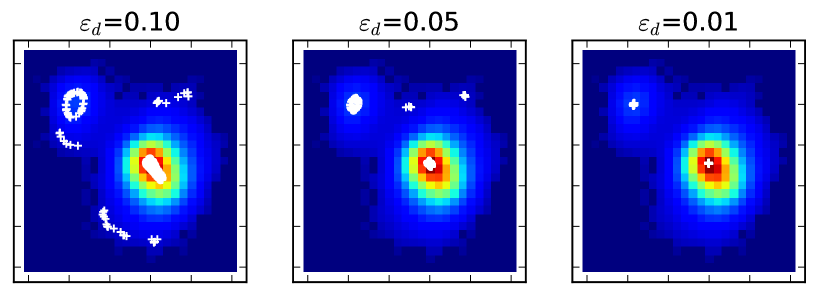
In the following we will use a Gaussian kernel function for the DENCLUE-based source deblending. We note that both $h$ and $\varepsilon_{d}$ have a significant impact on the final result of the deblending. The kernel width $h$ is relevant to the ‘scale’ of the deblended sub-clusters, indeed large values of $h$ will smooth high frequency signals, on the contrary small values will preserve small scale features. We have found that a value of kernel width $h$ of the order of $\simeq 0.1\times r_{max}$, provides good results in deblending sources, avoiding to fragment objects with complex morphology (such as spiral galaxies), and in separating close sources, even with a large difference in the integrated flux. The parameter $\varepsilon_{d}$ is responsible for the convergence of the fast hill climbing algorithm, hence for the determination of the position of the final attractor. A large value of $\varepsilon_{d}$, will allow to find local maxima related to noisy pixels, or morphological features of the source, a small value, on the contrary, will lead to track more significant maxima related to the core of the galaxy. We can see this clearly in Fig. 3, where we show the density attractors (white crosses) for different values of $\varepsilon_{d}$. We note that, as $\varepsilon_{d}$ is decreasing, all the attractors gets more and more tightly clustered around the two local maxima, corresponding to the two source cores.

Finally, in Fig. 4 we show how the deblending algorithm works. The left panel shows an image with three sources, two of which separated by a few pixels. The central panel shows the source detection with the DBSCAN threshold set to $K_{th}=1.5$, which finds only two sources. The right panel shows the image after the application of the DENCLUE-based deblending method with a Gaussian kernel function, with $h=$0.05$~{}r_{max}$.

3 application of DENCLUE to track spiral arms

Since the DENCLUE algorithm is able to track flux maxima in the 2D images, we decide to test whether this capability is able to track spiral arms too. As a first step we need to distinguish between cluster of density attractors related to the core of the galaxy, i.e. ‘core’ density attractors clusters, and ‘non-core’ density attractors clusters, that could be related to spiral arms patterns. We define the ‘core’ density attractors cluster as the cluster of attractors with the smallest distance form the galaxy centroid $(x_{c},y_{c})$, and fully contained within the galaxy effective radius $r_{eff}$.

The second step is to find the optimal configuration of the DENCLUE parameters for tracking spiral arms, i.e. we face a situation that is opposite to that of source debelnding. Indeed, in this case we are interested in finding attractors not only related to the core of the source, but also to fainter morphological features. As anticipated in the previous section, the bandwidth $h$, and the fast hill climbing threshold $\varepsilon_{d}$ play a relevant role in the extraction of the density attractors. Of course, $h$ has to be comparable with the scale of the feature that we want to extract, while $\varepsilon_{d}$ will tune the impact of the level of noise on the detection of the attractors. We have found that a Gaussian kernel with a bandwidth $h$ in the range [1.0,2.0] is able to track well spiral arms features, for the largest fraction of source sizes in our dataset, and that the optimal choice of $\varepsilon_{d}$ is in the range [0.1,0,2].

Even though we have identified an optimal range for both the two DENCLUE parameters, still it can happen that a given combination of $\varepsilon_{d}$ and $h$ is not able to find a cluster of attractors that meets the requirements to be a ‘core’ density attractors cluster as in the case of very noisy images. In order to mitigate such a possible bias we have implemented and automated iterative procedure to set the values of the two parameters of interest, $\varepsilon_{d}$ and $h$. The iteration is performed decreasing $\varepsilon_{d}$ of 5%, and increasing $h$ of 5%, until the ‘core’ cluster of density attractors has been found, or a maximum of $maxtrials=10$ iterations is reached.

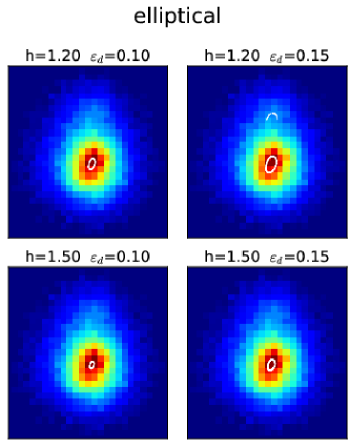
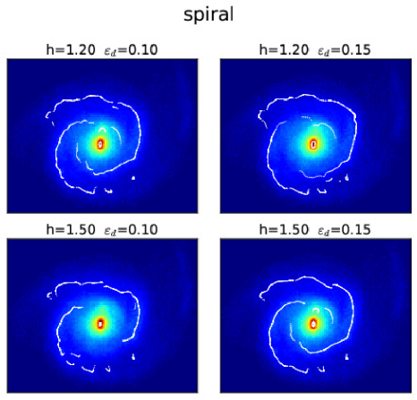
An example of this application is given in Fig. 5 where we show the typical case for an elliptical (left panels) and a spiral galaxy (right panels), for $h=1.2,1.5$ , and $\varepsilon_{d}=0.10,0.15$. It is clear that in the case of the elliptical galaxies ‘non-core’ density attractors are absent or rare, on the contrary, in the case of a spiral objects, we note a significant number of ‘non-core’ density attractors, following quite well the local maxima of the image related to the spiral arms.

Figure 6: Flow chart diagram showing the structure of the data processing pipeline

4 The ASTErIsM pipeline for the automatic galaxy shape identification

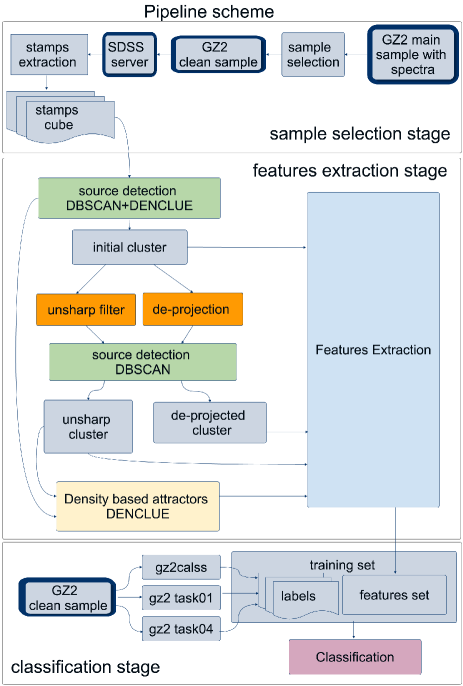
The ASTErIsM pipeline for the automatic galaxy shape identification consists of three different stages:

1. Sample selection.

2. Features extraction.

3. Classification.

a schematic view is shown in Fig. 6, and technical details about the code implementation are reported in App. A. In the following of the paper we will describe each stage of the pipeline, the extracted products, and their impact of the morphological classification.

Table 1: GZ2 decision tree tasks used in our sample selection

Task	question	Answer
01	Is the galaxy simply smooth and rounded, with no sign of a disk ?	A1.1 smooth
		A1.2 feature or disk
		A1.3 star or artifact
02	Could this be a disk viewed edge-on ?	A2.1 yes
		A2.2 no
04	Is there any sign of a spiral arm pattern ?	A4.1 yes
		A4.2 no

4.1 Sample selection

The galaxy images and the morphological classification have been taken from the Galaxy Zoo 2 (Willett et al., 2013) (GZ2) SDSS Main sample with spectroscopic redshifts. We have identified three relevant questions (or tasks) from the GZ2 decision tree (Willett et al., 2013), reported in Tab. 1, that are useful to identify a sub sample of well-identified spiral arms and elliptical objects. For each answer we have chosen, as decision variable, the debiased fraction of votes, that measures the agreement between a single user vote, and the best answer to that question (Willett et al., 2013). The following selection criteria have been used to select from GZ2 a sample of clean elliptical and clean spiral objects (see Tab. 1) :

• Elliptical galaxies cut : t01, A1.1$>0.9$

• Spiral galaxies cut: t01, A1.2$>0.9$ && t02, A2.2$>0.9$ && t04, A4.1 $>0.9$

producing a final clean sample of 24635 objects. Each object in sample has been labeled according to the class extracted from the column gz2class in the GZ2 catalog. All objects with the gz2class string starting with ‘E’ have been labeled as elliptical, and all the objects with string starting with ‘S’ have been labeled as spiral. In total we have 7186 elliptical objects and 17449 spiral objects.

For each object we have downloaded the g,r and i bands fits image from the SDSS, and a stamp of 100 by 100 pixels has been extracted, summing the three bands images, and centered on the source coordinates reported in the GZ2 catalog. We have decided to work with FITS image format, because compressed format such as JPEG, present interpolation features that might lead to spurious density attractors.

Table 2: Detailed description of the features. The first column reports the kind of cluster used to extract the image, the second the category of the features (clustering/morphology). The third column reports the name of the features group, and in round brackets is reported the section of the paper where the features are presented. The fourth columns reports the root name of the feature. The fifth column reports a flag, added to the name, with _ic corresponding to the initial cluster, _depr corresponding to the deprojected cluster, and _unsh corresponding to the unsharp cluster. The last column reports the number of features $N_{f}$ for each group.

Cluster	Category	Group (Sec.)	var. root name	flag	$N_{f}$
initial	clustering	Geometrical features (4.2.1)	geom	ic	7
	clustering	Hu moments of cl. contour (4.2.2)	cnt_log_Hu		7
	clustering	Hu moments of cl. image (4.2.2)	cl_img_log_Hu		7
	clustering	Hu moments of density attractors (4.2.4)	attr_log_Hu		7
	clustering	Hu moments of density attractors, polar coord. (4.2.4)	attr_polar_log_Hu		7
	morphology	Morphology of cl. image (4.2.3)	morph		10
unsharp	clustering	Geometrical features (4.2.1)	geom	unsh	7
	morphology	Morphology of cl. image (4.2.3)	morph		10
deprojected	clustering	Geometrical features (4.2.1)	geom	depr	7
	clustering	Hu moments of cl. contour (4.2.2)	cnt_log_Hu		7
	clustering	Hu moments of cl. image (4.2.2)	cl_img_log_Hu		7
	morphology	Morphology of cl. image (4.2.3)	morph		10
initial+	clustering	Radial distribution of non-core density attractors (4.2.4)	r_distr_attr	ic	7
unsharp	clustering	Angular distribution of non-core density attractors (4.2.4)	theta_distr_attr		5

4.2 Features Extraction

The features extraction stage consists of 4 main steps, and for each step a set of features is extracted, a schematic view of the stage is shown in the features extraction box of Fig. 6.

• initial clusters: The first step is used to detect the central source in the stamp, and to de-blend from possible nearby contaminating sources. If the source cluster has $r_{max}$ larger than 35 pixels, then the image stamp is rescaled in order to produce a source cluster with $r_{max}\leq 35$. We have checked that this rescaling has no impact on the quality of the extracted features, and has the only motivation to reduce the average computational time to $\simeq 3.5$ seconds per stamp.

  The source cluster produced at this stage is labeled as initial cluster, and the corresponding features are flagged with _ic string. We extract from this cluster a ‘cluster image’ by building an image with the same size of the original stamp, with null pixels, and setting the pixels belonging to the source cluster, to their actual flux value. This ‘cluster image’ is used as input for the extraction of the ‘de-projected’ cluster and of the ‘unsharp’ cluster’, and to extract image-related features.

• de-projected clusters: To extract the ‘de-projected’ cluster we de-project the initial cluster ‘cluster image’ by rotating and applying an affine transformation in order to map the galaxy shape to a shape that is as close as possible to circular. The re-pixelization of the image is based on third order spline interpolation, provided by the ndimage module from the scipy package (Jones et al., 2001). The detection process is again performed on this final image, and the ‘de-projected’ cluster with corresponding ‘cluster image’ are produced. The features are extracted and flagged with the string _depr

• unsharp clusters: To extract the ‘unsharp’ cluster we apply an unsharp filter to the initial cluster ‘cluster image’. This kind of filter is useful to enhance edges and high frequency features of the image. It is based on the subtraction between of a smoothed version of the original image, from the original one, producing and unsharp filtered image:

  $$I^{*}(x,y)=I(x,y)-u\cdot I_{smooth}(x,y)$$ (5)

  where the image is smoothed by a Gaussian filter with bandwidth $\sigma_{s}$, and the subtraction level is tuned by the parameter $u$. The value of $\sigma_{s}$ is chosen to be proportional to the Petrosian radius of the source (see 4.2.3 for a definition of the Petrosian radius). The detection process is again performed on the unsharp image, and the ‘unsharp’ cluster with the corresponding ‘cluster image’ are produced. The features are extracted and flagged with the string _unsh.

• density attractors As final steps we extract the density attractors from the ‘initial cluster’, using the pixels that are common both to the ‘initial’ and to the ‘unsharp’ cluster, i.e. the convolution equation for the DENCLUE algorithm will read:

  $$f(p_{j})\propto\sum_{i=1}^{n}G\big{(}\frac{\mathbf{q}_{j}-\mathbf{q}_{i}}{h}\big{)}I(\mathbf{q}_{i})$$ (6)

  where $j\in$ ‘initial cluster’, and $i\in$ ‘unsharp cluster’. This choice allows to avoid that some attractors will match the edges of the source clusters, lowering the possibility to detect attractors not related to spiral arms structures.

We will distinguish the extracted features in two categories:

• clustering-related: These features can be evaluated only if a cluster is extracted, and are evaluated from the information stored in the source cluster, or from the extracted cluster image.

• morphological: These features have already been used in the literature (see Sec. 4.2.3), and could be evaluated without the need to extract the source cluster.

All the features, are summarized in Tab 2. The feature name is built according to the following scheme: root_name+specific_name+flag. In the following, if not specified otherwise, we will refer to the specific name.

4.2.1 Geometrical Features

Since the DBSCAN cluster shape is arbitrary, i.e. there is no constraint coming from convolution with a predefined shape, the extracted cluster preserve as much as possible the actual shape of the source. For this reason, we have identified a set of features that maximize the cluster geometrical information, measured from the position of the source cluster points, and of the contour points:

• geom_pix_size - the number of pixels of the cluster.

• geom_r_max - the $r_{max}$ of the cluster.

• geom_ecc - the eccentricity of the cluster containment ellipsoid (see Sec.2.1).

• geom_comp - the geometrical compactness, defined as $P^{2}/A$, where $P$ is the contour perimeter (i.e. the number of pixels flagged as contour), and $A$ is the total number of pixels of the cluster.

• geom_ar - the aspect ratio of the minimal rectangular box enclosing the source cluster.

• geom_contour_ratio - the contour ratio defined as $P_{box}/P$, where $P_{box}$ is the contour perimeter of the minimal rectangular box enclosing the cluster.

• geom_area_ratio - the area ratio, defined as $A_{box}/A$, where $A_{box}$ is the area of the minimal rectangular box enclosing the cluster.

4.2.2 Invariant Hu moments

We can increase the amount of information provided by the DBSCAN clusters, by evaluating the Hu moments (Hu, 1962), which are a set of 7 geometrical moments that are invariant under scaling, rotation, and translation. The complete definition is reported in Appendix B. The following features are extracted:

• cnt_log_Hu_[0-6] - the logarithm of Hu moments of the cluster contour.

• cl_img_log_Hu_[0-6] - the logarithm of Hu moments of the cluster image.

Figure 7: The radial distribution of the density attractors for the detections of the two galaxies shown in Fig. 5, for the four different combinations of $h$ and $\varepsilon_{d}$. The data points are plotted as as vertical sticks on the x axis. The solid lines represent the density function of the data points, estimated using a Gaussian kernel. Left panels: radial distribution of core (orange) and non core (green) density attractors for the elliptical galaxy case. Right panels: the same as in the left panels, for the spiral galaxy case.

4.2.3 Morphological Features

We extract, from the source cluster image, also a set of morphological features already presented in the literature. A detailed description of these features is given in Conselice (2003); Lotz et al. (2004); Conselice et al. (2008). In the following we give only a brief description. An important point, that differs from previous application of these features, is that in our case we do not need to deal with the background. Indeed our cluster image stores only the pixels belonging to the detected source cluster, hence all the background pixels are already removed from the image.

• morph_gini - the Gini factor. The Gini factor (Lotz et al., 2004) indicates the distribution of the light among pixels. A value of Gini equal to 1 would indicate that all the light is concentrated in one pixel, on the contrary, a lower value would indicates that the light is distributed more evenly amongst the pixels, with Gini factor equal to 0, if all the pixels have the same flux value.

• morph_M20 - the normalized second-order moment of the 20% brightest pixels of the galaxy: this feature has been introduced by Lotz et al. (2004), and it is computed starting from the total second order moment

  $$M_{tot}=\sum_{i}^{n}M_{i}=\sum_{i}^{n}I_{i}[(x_{i}-x_{c})^{2}+(y_{i}+y_{c})^{2}],$$ (7)

  where $x_{c},y_{c}$, represent the source cluster centroid, and $I_{i}$, is the flux of each source cluster pixel, with coordinate $x_{i},y_{i}$. $M_{20}$ is defined as the normalized second-order moment of the 20% brightest pixels of the galaxy computed as:

  $$M_{20}=\log 10\frac{\sum_{i}M_{i}}{M_{tot}},\textnormal{While}\sum_{i}I_{i}<0.2I_{tot}$$ (8)

• morph_conc_1,morph_conc_2 the concentration indices, defined as:

  $$C1 = \log(r_{80}/r_{20}),$$ (9)

  $$C2 = \log(r_{90}/r_{50})$$

  where $r_{x}$ represents the radius of the circular discs containing a x% and of the total cluster flux.

• morph_r_80_to_r_max, morph_r_20_to_r_max- the ratio of $r_{80}$ to $r_{max}$, and $r_{20}$ to $r_{max}$

• morph_r_Petrosian_to_r_max - the ratio of the Petrosian radius to the deprojected source cluster $r_{max}$. To determine the Petrosian radius we use the same definition as reported in Conselice et al. (2008). Let $\mu(r)$ be the surface brightness at the radius $r$, and $\mu(<r)$ the integrated surface brightness within $r$. We define $r_{\eta}$ as the radius at which $\mu(r_{\eta})/\mu(<r_{\eta})=\eta$, and the Petrosian radius as $R_{p}=1.5r_{\eta=0.2}$

• morph_clumpiness - the clumpiness index, defined as:

  $$S=10(\frac{\sum_{i}^{n}|I_{i}-I_{i}^{*}|}{\sum_{i}^{n}|I_{i}|}\big{)}$$ (10)

  where $I^{*}$ is the cluster image smoothed with a Gaussian Kernel, with a bandwidth $w=s*R_{p}$, where $s$ is a factor ranging in $0.0-1.0$.

• morph_asymm - the asymmetry index, defined as:

  $$A=min\big{(}\frac{\sum_{i}^{n}|I_{i}-I_{180,i}|}{\sum_{i}^{n}|I_{i}|}\big{)}$$ (11)

  where $I_{180}$ is the cluster image rotated 180 degrees around the cluster centroid.

Figure 8: Distribution of features derived from radial and angular distribution of non-core density attractors, showing the separation between the elliptical and spiral classes, for the objects in our sample, averaged for four different values of the DENCLUE parameter $h$ = [1.0,1.2,1.4,1.6]. Left panels: distribution of r_distr_attr_non_core_ratio and r_distr_att_delta_r_non_zero. Right panels: distribution of theta_distr_attr_sig and theta_distr_attr_delta_theta_non_zero. The solid lines represent the density function, estimated using a Gaussian kernel.

4.2.4 Features from radial distribution of the density attractors

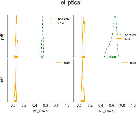
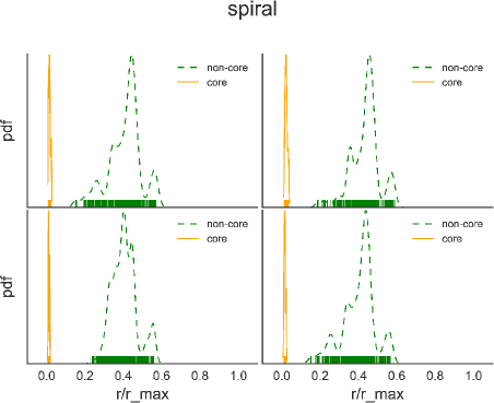
In general, elliptical galaxies have only one cluster of attractors corresponding to the core of the galaxy, and zero or small attractor clusters outside. On the contrary, spiral galaxies in addition to the core cluster, have clusters of attractors that tracks the spiral arms, this reflects in a strong difference in the radial and angular distribution of the attractors. A clear example is given in Fig. 7, where we show the radial distribution of the density attractors for the detections of the two galaxies shown in Fig. 5. The radial distribution of the non-core attractors (green lines) is quite different in the two cases of elliptical and spiral objects. The former has zero, or very little contribution, the latter shows a significant contribution. In particular we note that in the case of elliptical, when non-core density attractors are found, they are distributed with a narrow peak, while elliptical have a broader distribution. To make the comparison more homogeneous, we normalize the radial coordinate as $r=r/r_{max}$, where $r_{max}$ is the most distant point in the source cluster, from its centroid. Hence, we can use a statistical characterization of these distributions in order to provide important classification features. In the following we list and explain the extracted features. The root name of the radial distribution variables is r_distr_attr_, and that for the angular distribution variable is theta_distr_attr_, and in the following of this section we report only the specific name. We remind that all the features extracted from the radial and angular distribution of the density attractors, are evaluated from the distribution of only non-core density attractors: The features evaluated for the radial distribution are:

• non_core_ratio - the ratio of number non-core density attractors to the total number of points in the source cluster defined as:

  $$\texttt{non\_core\_ratio}=\frac{N_{non-core}}{N_{source}}$$ (12)

  where $N_{non-core}$ is the total number of points in the non-core clusters, and $N_{source}$ is the total number of points in the source cluster.

• mode - the mode of the radial distribution.

• sig - the standard deviation of the radial distribution.

• skew - the skewness of the radial distribution.

• skew_p_val - the two-sided p-value for the skewness test.

• kurt - the kurtosis of the radial distribution.

• delta_r_non_zero - the difference. between the largest and the smallest value of $r$, where the distribution is larger than zero.

The features evaluated for the angular distribution are:

• sig - the standard deviation of the angular distribution.

• skew - the skewness of the angular distribution.

• skew_p_val - the two-sided p-value for the skewness test.

• kurt - the kurtosis of the angular distribution.

• delta_theta_non_zero - the difference. between the largest and the smallest value of $theta$, where the distribution is larger than zero.

Moreover, we extract also the Hu moments for the density attractors both in Cartesian and polar coordinate, attr_log_Hu_[0-6] and attr_polar_log_Hu_[0-6] respectively.

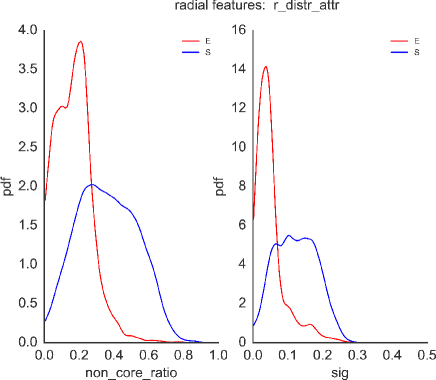
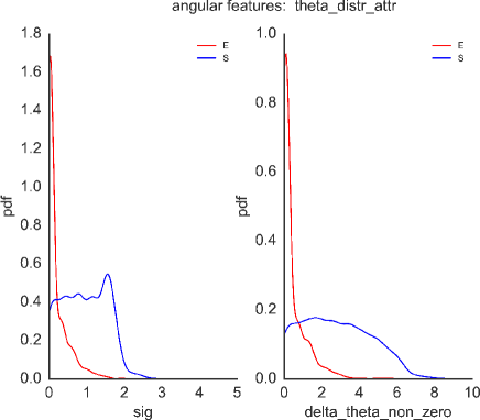
Left panels of Fig. 8 show the distribution of the radial features non_core_ratio and sig, for the objects in our sample, averaged for four different values of the DENCLUE parameter $h$ = [1.0,1.2,1.4,1.6]. Both spiral and elliptical objects have the mode of the distribution at $\texttt{non\_core\_ratio}\simeq 0.2$, but elliptical galaxies, as expected, are characterized by lower values of non_core_ratio, indeed $\simeq 70\%$ of the elliptical have a value of non_core_ratio below the mode, while $\simeq 80\%$ of the spiral have a value of non_core_ratio above the mode. A further difference is given by width of the radial distribution, indeed we observe that elliptical objects are characterized by values of standard deviation of the radial distribution, sig, close to zero, while spiral ones have larger values. Again, this behavior is in agreement with our expectations, indeed, spiral arms will have density attractors that typically will span the largest fraction of the radial extension of the galaxy, while density attractors in elliptical will be related mostly to noisy pixels, or to unresolved sources (i.e. cases in which the deblending did not succeed.), or to rings in polar ring galaxies or lensing signals, and will have a narrower radial extent. This effect has an impact on the angular size of the density attractors and it is confirmed by the plots in the right panels of Fig. 8, where we show the distributions of the angular features sig and delta_theta_non_zero. Both the plots show how in the case of elliptical objects the angular size of the density attractors peaks close to 0, while in the case of elliptical objects it reaches a much larger angular size.

4.3 Final features set

In total we have 105 features ($N_{f}$) extracted by our pipeline. We have run the pipeline with four different values of the DENCLUE parameter $h=[1.0,1.2,1.4,1.6]$ . This parameter, as already discussed, has a important impact on the scale of the morphological structures that will be found by the attractors. The other parameters used for the feature extraction are reported in Tab. 3. Fore each feature, we compute the average of the four values obtained with the different h values. We will refer to this set as the h-averaged features set, and it will be used in the classification analysis presented in the next section. A fits table version of this features set is available as supplementary material (see App. C)

Table 3: Pipeline parameter space

Pipeline task	parameter	values
background est.	$N_{bkg}$	3.5
dbscan detection	$K_{th}$	1.5
denclue deblending	$h$	0.15$\times r_{max}$
	$\varepsilon_{d}$	0.01
density attractors	$h$	1.00,1.20,1.40,1.60
	$\varepsilon_{d}$	0.10
Unsharp Filtering	$u$	0.5
	$\sigma_{s}$	1.0 $\times R_{p}$

5 Training Sets

We decided to test our classification against the class labels reported in the gz2class column of the GZ2 catalog, and against the labels extracted from the answers to tasks t01 and t04 of the GZ2 decision tree (see Tab. 1). We have prepared three sets of training objects (see Tab. 4):

• The GZ2 class set of training objects is based on the class extracted from the column gz2class in the GZ2 catalog, and the features from the h-averaged set. All objects with the gz2class string starting with ‘E’ have been labeled as elliptical, and all the objects with string starting with ‘S’ have been labeled as spiral.

• The two sets of training objects, GZ2 task 01 and GZ2 task 04, are based on the labels extracted from the answer to tasks t01 and t04. Also in this case we use the features from the h-averaged features set. We note that in our selected sample of objects there are no entry for the $A1.3$ answer, corresponding to the start or artifact category.

A fits table version of these training features set is available as supplementary material (see C)

6 Supervised ensemble classification

Supervised machine learning (ML) represents a powerful tool to infer a classification function from a labeled training data set. One of the possible method used is given by the so called "Ensemble" methods, that rely on the combination of several learners. The outcome from the combination of several learners will be much more robust than that from a single one. Among the ‘Ensemble’ family, there is a further separation based on the relation among the estimators in the ensemble, and their impact on the classification error:

• averaging based methods: based on large number of complex, and mutually independent estimators. Since each estimator is ‘complex’, the error bias is low, but the variance can be large, and it is reduced by the averaging.

• boosting based methods: based on sequential construction of simple estimators. The estimators are ‘weak’, hence they have large bias, but a small variance. The combination of the estimators leads to a decrease in the bias.

We use two different supervised ensemble classification algorithms, Random Forest (Breiman, 2003) belonging to the family of averaging based methods, and Gradient Boosting Friedman (2001) belonging to the family of boosting based methods. For both the classifier we have used the implementation provided by the scikit-learn (Pedregosa et al., 2011) python package

Figure 9: Diagram for the supervised classification process.

Table 4: Sets of training objects

Name	class labels	size
GZ2 classes	E,S	24635
GZ2 task 01	A1.1,A1.2	24635
GZ2 task 04	A4.1,A4.2	21730

6.0.1 Gradient Tree Boosting

The Gradient Tree Boosting (GB) method, is based on the idea of building a strong learner from the combination of several weak learners. Weak learners are decision trees, and are added together sequentially. At each stage of the process, a further decision tree is added to the ensemble, and the newly generated decision tree is trained in order to minimize a loss function. This result is achieved by making the new decision tree maximally correlated with the negative gradient of the loss function. A detailed review of GB methods is given in Natekin & Knoll (2013)

6.0.2 Random Forest

Random Forest (RF) is an ensemble classification method, based on averaging. It has been successfully applied to different astrophysical subjects, such as classification of periodicity in variable stars (Dubath et al., 2011). Trees are constructed from bootstrapped samples of the original training set. A randomize set has the same size than the original training set, but some of the elements of the original training set may appear multiple times, while others are missing. The original elements missing in the bootstrapped sample will constitute the so called out-of-bag (OBB) sample.

If our training set has $N_{f}$ features, each decision tree will be built from a random subsample of features whose number is $n_{f}<<N_{f}$. Trees are grown deep, hence will have low bias but a large variance. The averaging over a large number $M$ of trees, has the goal to reduce the variance of the final model.

6.1 classification metrics

To express the capacity of the model to predict correctly a given morphology, we need to provide a metric of the classification results. We will use the following indicators:

• accuracy: i.e., the ratio of the total number of correctly classified objects, to the total number of objects in the sample

• precision or purity, defined as $P=\frac{TP}{TP+FP}$, where $TP$ are the true positive, and $FP$ are the false positive. This indicator gives the fraction of correctly classified objects, for a specific class.

• recall or completeness, defined as $R=\frac{TP}{TP+FN}$, where $FN$ are the false negative. This indicator gives the fraction of correct prediction for a specific class, in terms of the total number of object actually belonging to that class.

7 Classification strategy

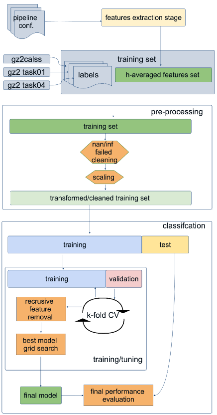
Even though ML classification methods are quite powerful, their application requires well defined strategies that allows to fit the ‘model’ to a set of training data, with reliable predictions on general data (never used in the training process) and without overreacting to the noise present in the training set. To accomplish this goal we need to tune the model in such a way that it is not too simple, i.e. suffering from underfitting the data (high bias), or too complex hence suffering from overfitting the data (high variance). Our ML strategy is based on two stages, a pre-processing stage, and a classification stage, and the corresponding pipeline has been implemented around te scikit-learn framework (Pedregosa et al., 2011). A schematic view is shown in Fig. 9.

7.1 data pre-processing

• nan/inf, failde, cleaning We remove all the entries with features having non-valid values, or the entries corresponding to failed featured extraction.

• scaling We scale the features in our features set using the procedure of the standardization (StandardScaler method from scikit-learn ), i.e. the features are centered at mean 0, with a standard deviation of 1. Even though this step is not mandatory for the ensamble classification methods that we will use, it allows a better comparison with other ML models.

7.2 classification

• train/test partitioning the training set is split in training and a test set, with a ratio of $80\%$ training, $20\%$ test. The data in the test set will never be seen by the model training process, and will give our final benchmark for the model performance

• k-fold cv for model tuning We split our training set in training and validation set, using a k-fold cross validation method (StratifiedKFold method from scikit-learn) that splits randomly the training set into k folds without replacement, where k-1 are used for the training and one for the validation. In particular we use a stratified k-fold cross validation, which preserves in each fold the original relative ratios of the classes.

• model tuning: dimensionality reduction We use a recursive feature elimination based on the accuracy ranking from the cross-validate score on the model, using the the RFECV method scikit-learn.

• model tuning: regularization We regularize the model by optimizing the number of decision trees, using the accuracy score from a cross-validated grid-search based on the GridSearchCV method from scikit-learn.

• final performance the final model is tested on the test stet, whose data have never been used in any of the training steps before.

Table 5: Classification metrics for the GZ2 class test set: statistics come from the trials corresponding to 100 repetitions of the classification experiment. The firs column gives the name of the classifier. The second column reports the accuracy. The third columns shows the morphological classes. The fifth and sixth, report the precision and the recall, respectively. The las column reports the average number of features, used in the classification, after the feature selection

classifier	accuracy	Class	precision	recall	$<N_{f}>$	Test size
RF	$0.926\pm 0.003$ max=0.933	E	$0.889\pm 0.008$	$0.853\pm 0.008$	43.89	4927
		S	$0.941\pm 0.003$	$0.956\pm 0.004$
GB	$0.935\pm 0.003$ max=0.946	E	$0.898\pm 0.008$	$0.878\pm 0.008$	52.85
		S	$0.950\pm 0.003$	$0.959\pm 0.004$

Figure 10: distribution of accuracy, purity, and completeness, for the RF (upper panels) and GB (bottom panels) classifier, for the GZ2 class test set trials, corresponding to the 100 repetitions of the classification experiment.

8 Classification performance

In order to assess the classification performance of our method we repeat 100 times a classification experiment, using the methodology describe in 7.2, and illustrated in the classification box of Fig. 9. Before running the classification we pre-process the data as reported described in 7.1. The cleaning process removes only two entries from our training set, hence we have final number of 24633 objects in the gz2class training set.

Figure 11: Top 20 ranked features importances, for RF (left panel) and GB (right panel), classifiers, averaged over the 100 classification experiment repetitions with the GZ2 class test set.

Table 6: Classification metrics for GZ2 task for the task 01 and the task 04 test sets, for the RF classifier. Statistics come from the trials corresponding to 100 repetitions of the classification experiment. Column description as in Tab. 5

classifier	GZ2 Task	accuracy	Answer	precision	recall	$<N_{f}>$	Test set size
RF	t01	$0.922\pm 0.004$ max=0.931	A1.1	$0.887\pm 0.008$	$0.847\pm 0.009$	43.2	4927
			A1.2	$0.936\pm 0.004$	$0.954\pm 0.004$
			A1.3	-	-
	t04	$0.929\pm 0.003$ max=0.936	A4.1	$0.949\pm 0.003$	$0.964\pm 0.003$	39.9	4346
			A4.2	$0.82\pm 0.01$	$0.77\pm 0.01$

Table 7: Same as in Tab. 5 for the GB classifier.

classifier	GZ2 Task	accuracy	Answer	precision	recall	$<N_{f}>$	Test set size
GB	t01	$0.930\pm 0.003$ max=0.936	A1.1	$0.892\pm 0.007$	$0.869\pm 0.009$	52.3	4927
			A1.2	$0.945\pm 0.004$	$0.955\pm 0.003$
			A1.3	-	-
	t04	$0.931\pm 0.003$ max=0.940	A4.1	$0.954\pm 0.003$	$0.963\pm 0.003$	58.6	4346
			A4.2	$0.82\pm 0.01$	$0.79\pm 0.02$

8.1 GZ2 classes training set

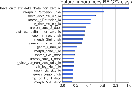
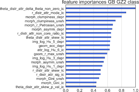
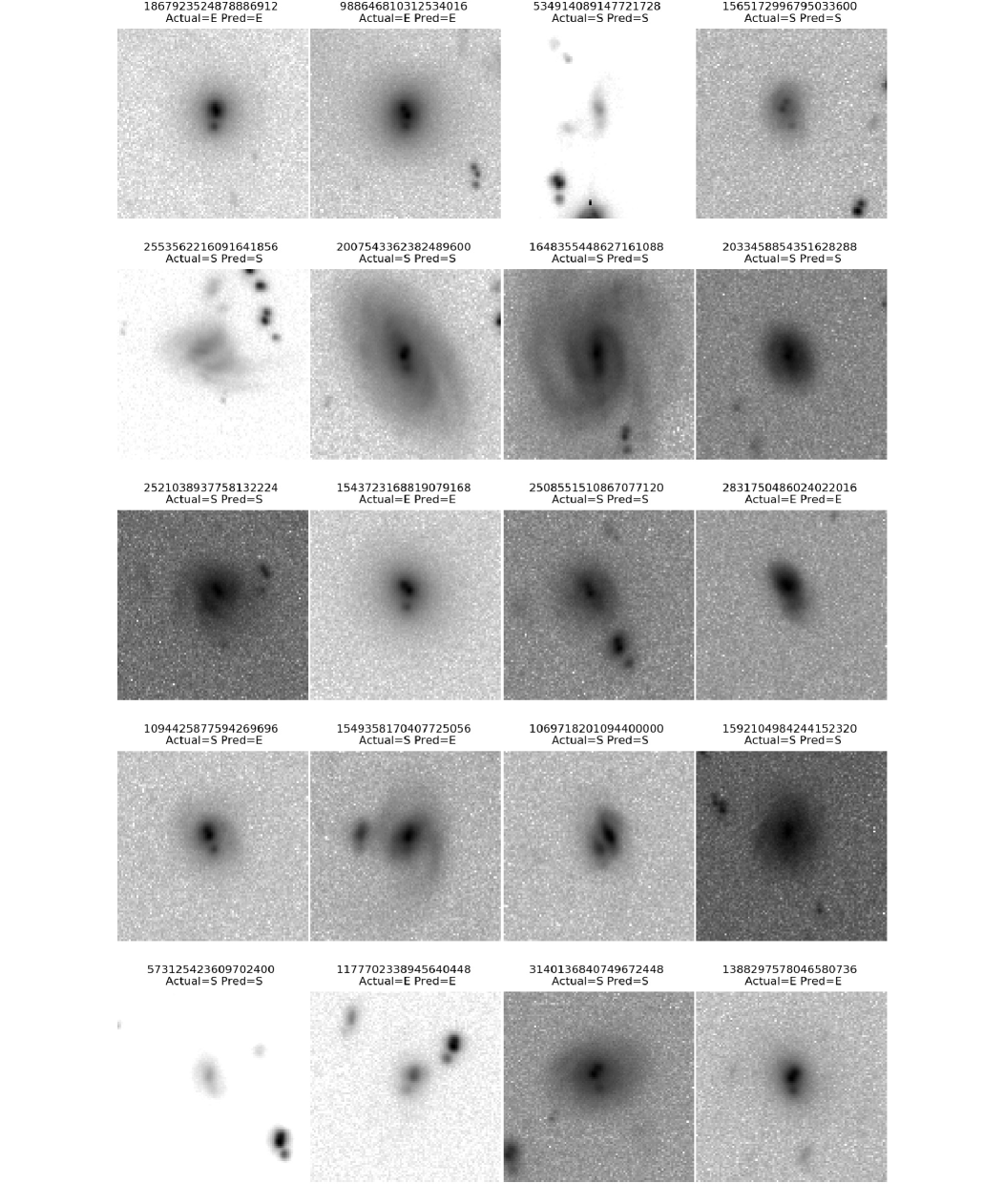
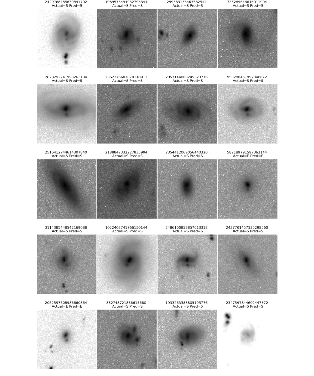
The train/test partitioning is done with a ratio of $80\%$ training $20\%$ test, for a corresponding number of 19706 objects for the training set, and 4927 for the test set. The results for the test set classification are reported in Tab. 5, and shown in Fig. 10. The average accuracy of the classification is $\simeq 93\%$ for the RF classifier and $\simeq 94\%$ for the GB classifier. Precision and recall for both the elliptical and spiral classes are also reported. The overall performance is very good if we consider that the use a quite large test set of $~{}5000$ objects, and that by repeating the experiment 100 times we give also a good estimate of the error intrinsic to the model and to the data. It is interesting to understand which feature have the highest classification power. We rank the features importance using the feature_importances_ attribute, that is implemented in all the tree-based models of scikit-learn. The feature_importances_ is evaluated according to the so called ‘Gini importance’ or ‘mean decrease impurity’ (Breiman et al., 1984). This method defines the importance as the total decrease in node impurity ,weighted by the probability of reaching that node, and averaged over all trees of the ensemble. The results are reported in Fig. 11, where we plot the 20 top-ranked features for both the RF (left panel) and the GB (right panel) classifier. We report the importance averaged over the outcomes of the 100 repetitions of our classification experiment. We note that both in the case of RF and GB classifier, the most important features is theta_distr_attr_delta_theta_non_zero_ic, meaning that the angular distribution of the attractors is storing the largest fraction of discrimation power among all the features. The second most important feature, in the case of the RF classifier, is the Petrosian Radius of the ‘unsharp’ cluster, and the most important features from the radial distribution of the ‘density’ attractors is the r_distr_attr_sig_ic. In the case of the GB classifier, the most important features from the radial distribution of the ‘density’ attractors is r_distr_attr_mode_ic, ranking in the second position. We report in Fig. 12 and Fig. 13, some of the images from the test set, with their GZ2 specobjid identifier, and both the actual and predicted classes.

8.2 GZ2 tasks training sets

As further experiment to assess the discrimination power of our classification technique we have tested our model against the labels extracted from the answers to tasks t01 and t04. Results are summarized in Tab. 7 and Tab. 7. We note a very good agreement between the outcome of our classifier and the GZ2 votes, with our GB classifier showing an average accuracy of $\simeq 93\%$ both for the task t01, and the task t04.

8.3 Comparison with similar works

In the last years several methods, based on the application of machine learning, have been used to classify galaxy morphology. Banerji et al. (2010) and Dieleman et al. (2015) have used artificial neural networks (ANN), while Huertas-Company et al. (2008); Huertas-Company et al. (2011) have used Support Vector Machine (SVM) classifier and Ferrari et al. (2015) have used Linear Discriminant Analysis (LDA) classifier.

Banerji et al. (2010) have used a sample of 75000 object (50000 for training and 25000 validation) from the Galaxy Zoo 1 catalog, to train a neural network in order to reproduce the human classification in early type, spiral, and point source/artifact . The authors obtained the best performance (better than 90%) in terms of agreement with human classification, when adding $(g-i)$ and $r-i$ colors, to features deriving from de Vaucoleurs and exponential profile fitting, and quantities deriving form adaptive moments and image texture. Performance of Banerji et al. (2010) are comparable with our results, with the difference that we use a larger amount of features, but we do not use color information.

Dieleman et al. (2015) used a a training set of 61578 images, and 79975 images for the validation, from Galaxy Zoo 2, to train their neural network to reproduce the human answers to the 11 tasks in Galaxy Zoo 2. The results presented by the authors refers only to a sub sample of the test set images with at least 50 percent of participant answering. In our work we have investigated two task in common with Dieleman et al. (2015): t01 and t04. Dieleman et al. (2015) evaluated their classification metrics in 10 different bins of participants agreement. For the task t01 , they report an agreement-averaged accuracy of $87.79\%$ for a test set of 6144 objects, and an agreement-averaged accuracy of $82.52\%$ for task t04, with a test set of 2449 objects. We note that for both of the tasks our classification pipeline gives an accuracy higher than that obtained by (Dieleman et al., 2015).

In general, compared to result from neural network, we observe that our classification technique performs very well, with the advantage that we can have a direct understanding of the weight of the input features on the final classification.

Finally we compare our result to those presented by Ferrari et al. (2015) and Huertas-Company et al. (2008); Huertas-Company et al. (2011).

Huertas-Company et al. (2008) classified a test set of $\simeq 1500$ objects from SDSS, and they obtained a mean accuracy of $\simeq 80\%$ for the early-vs-late type classification, using a SVM classifier, hence our classification performance seems to show a significantly larger accuracy. In a more recent work, Huertas-Company et al. (2011) analyzed a large sample of $\simeq 700$k galaxies from the SDSS DR7 spectroscopic sample, and they provided a probability of the object to belong to a given class. Since their classification scheme is based on 4 morphological types, it is not straightforward to compare Huertas-Company et al. (2011) results to ours.

Among the works found in the literature the analysis approach presented in Ferrari et al. (2015) is the one that is closest to ours, indeed the authors use purely morphometric information (no colors), and a classifier (LDA) rather than a neural network. Ferrari et al. (2015) analyzed three different data sets, the EFIGI catalog (Baillard et al., 2011), the Nair and Abraham (Nair & Abraham, 2010) catalog, and the SDSS DR7 complete Legacy sample. Their code, Morfometryka (Ferrari et al., 2015) uses as input features standard morphological coefficients, with new parameters such as the image entropy index $H$, and the spirality $\sigma_{\phi}$. This last parameter is able to compute the amount non radial patterns in the image, by computing the gradient of the polar-projected image. Performance of accuracy obtained by Ferrari et al. (2015) refers to the classification of a sub-samples of their catalog having a Galaxy Zoo 2 classification, and these authors classify against the elliptical-vs-spiral labels like in our case. The performance of their classification scheme, in terms of accuracy, are comparable to ours, with the difference that they use a larger data-set, but they rely only on 10-fold cross-validation, without a specific test set. Moreover, we note that in their case the largest importance is obtained by features related to light concentration, unlike in our case, where the most important features are related to the angular distribution of density attractors, both for the RF, and the GB classifiers.

9 Conclusions and future developments

The results presented in this work show the successful application of ASTErIsM software, based on topometric clustering algorithms (DBSCAN and DENCLUE), to automatic galaxy detection and shape classification. For the detection process we have found that:

• DBSCAN clusters usually preserve the actual shape of the source, allowing to follow quite well the contour of any arbitrary morphology.

• When sources are ‘confused’, the application of the DENCLUE algorithm allows to deblend them.

We have verified that, in addition to deblending, the density attractors evaluated by the DENCLUE algorithm track quite well spiral arms features, and we have found that:

• In general, elliptical galaxies have a single cluster of e density attractors related to the core of the galaxy, while spiral galaxies have additional ones related to the presence of spiral arms.

• The radial and angular distribution of the density attractors are very different in the case of spiral and elliptical objects.

Basing on these results we have defined a new set of features for the galaxy classification, that maximize the information given by the DBSCAN clusters (see Sec. c. 4.2.1, 4.2.2), and the DENCLUE density attractors (see Sec. 4.2.4). In addition to these clustering-related features we have also evaluated classical morphological features (see Sec. 4.2.3).

We have tested the classification performance of the features evaluated by our pipeline, on a training set of about 24k objects, selected from GZ2 SDSS main sample with spectroscopic redshift, using a Random Forest and a Gradient Tree Boosting classifier. We have tested the classification performance against the GZ2 classification in elliptical vs spiral classes, and against the answers to the task t01 and t04 of the GZ2 decision tree. In general the accuracy of our classification, for the test set, is $\simeq 93\%$ with a performance comparable to other approach based on ANN (Dieleman et al., 2015; Banerji et al., 2010) or based on SVN and LDA classifiers (Huertas-Company et al., 2008; Ferrari et al., 2015).

As future developments, we would like to investigate how deal with the classification of a larger number of morphologies, in particular investigating the capabilities to detect bars and bulges. Moreover, we aim at using the density attractors as a baseline to fit spiral arms, and investigating how this compare to human identified arms. We plan also to improve the DENCLUE-based deblending, using a ML approach, adding a feedback between density attractors extracted in the deblending process, and the density attractors extracted in the morphological feature extraction process.

Appendix A Technical details about the ASTErIsM pipeline implementation

The ASTErIsM software is implemented as a python 2.7 package. The code is object oriented. All the algorithms for clustering and features extraction have been implemented from the scratch. The kernel computation in the DENCLUE algorithm has been written in Cython (Behnel et al., 2011) to speed up the computational time. Some image processing tasks are performed using the ndimage package from the SciPy library (Jones et al., 2001), the scikit-image (van der Walt et al., 2014) package, and the Python wrapper of the OpenCV library (Bradski, 2000). The I/O operations for the fits file use the PyFits library. The classification module uses the scikit-learn Python package (Pedregosa et al., 2011). The graphical output, including the figure in the present paper, have been implemented using the Matplotlib library (Hunter, 2007) and the Seaborn (Waskom et al., 2015) library. The code will be available at https://github.com/andreatramacere/asterism.

Appendix B Hu moments

The two-dimensional $(p+q)-th$ order geometric moment of a two-dimensional distributions of points $(x_{i},y_{i})$ is defined as:

$$m_{pq}=\sum_{i=0}^{N-1}\sum_{j=0}^{N-1}(x_{j})^{p}(y_{j})^{q}$$ (13)

If we are interested in the moments of a digital image whose pixels have coordinates $(x_{i},y_{i})$, and fluxes $f(x_{i},y_{i})$ then the previous equation reads:

$$m_{pq}=\sum_{i=0}^{N-1}\sum_{j=0}^{N-1}(x_{j})^{p}(y_{j})^{q}f(x_{i},y_{i})$$ (14)

The centroid can be evaluated as: $\bar{x}=m_{10}/m_{00},\bar{y}=m_{01}/m_{00}$, and the central moments as:

$$\mu_{pq}=\sum_{i=0}^{N-1}\sum_{j=0}^{N-1}(x_{j}-\bar{x})^{p}(y_{j}-\bar{y})^{q}$$ (15)

or in the case of digital image as:

$$\mu_{pq}=\sum_{i=0}^{N-1}\sum_{j=0}^{N-1}(x_{j}-\bar{x})^{p}(y_{j}-\bar{y})^{q}f(x_{i},y_{i})$$ (16)

The normalized central moments are given by:

$$\eta_{ji}=\frac{\mu_{ji}}{\mu_{00}^{(1+\frac{i+j}{2})}}$$ (17)

As proved by Hu (1962), it is possible to obtain moments that are invariant under translation, scaling and rotation:

$$Hu[0] = \eta_{20}+\eta_{02}$$ (18)

$$Hu[1] = (\eta_{20}+\eta_{02})^{2}+4\eta_{11}^{2}\$$

$$Hu[2] = (\eta_{30}+3\eta_{12})^{2}+(3\eta_{21}+\eta_{03})^{2}$$

$$Hu[3] = (\eta_{30}+\eta_{12})^{2}+(\eta_{21}+\eta_{03})^{2}$$

$$Hu[4] = (\eta_{30}-3\eta_{12})(\eta_{30}+\eta_{12})^{2}$$

$$[(\eta_{30}-3\eta_{12})^{2}-3(\eta_{21}+\eta_{03})^{2}]$$

$$+(3\eta_{21}-3\eta_{03})(3\eta_{21}+\eta_{03})$$

$$[3(\eta_{30}+\eta_{12})^{2}-(\eta_{21}+\eta_{03})^{2}]$$

$$Hu[5] = (\eta_{20}-\eta_{02})[(\eta_{30}+\eta_{12})^{2}-(\eta_{21}+\eta_{03})^{2}]+$$

$$4\eta_{11}(\eta_{30}+\eta_{12})(\eta_{21}+\eta_{03})$$

$$Hu[6] = (3\eta_{21}-\eta_{03})(\eta_{21}+\eta_{03})$$

$$[3(\eta_{30}+\eta_{12})^{2}-(\eta_{21}+\eta_{03})^{2}]$$

$$-(\eta_{30}-3\eta_{12})(\eta_{21}+\eta_{03})$$

$$[3(\eta_{30}+\eta_{12})^{2}-(\eta_{21}+\eta_{03})^{2}]$$

Appendix C Data products and tables

We provide a fits table of the training sets used in this work. The table contains the columns concerning the h-averaged features set, as well as those corresponding to gz2class E/S classification, and those corresponding to the the task t01 and t04 of the GZ2 decision tree. A description of the table is given in Tab 8

Table 8: Description of the columns for the online training set. For the features names we report the string for root variable name and the string for the flag corresponding to the type of cluster used to extract the features. The specific name of the variable is left as a blank space. Please, refer to 4.2 and Tab. 2 a specific description of the features names

Col name	Col description
specobjid	match to the DR8 spectrum object
ra	right ascension [J2000.0], decimal degrees
dec	declination [J2000.0], decimal degrees
gz2class	gz2class label for the E/S classification
t01	label for the t01 the GZ2 decision tree
t04	label for the t04 the GZ2 decision tree
id_ cluster	The id of the ASTErIsM detected cluster corresponding to the GZ2 source.
	If negative, it means no source was detected, or source detection failure.
geom_ _ic	(7 columns) geometrical features for the ‘initial ’ cluster(see. 4.2, 4.2.1, and Tab. 2)
geom_ _derp	(7 columns) geometrical features for the ‘deprojected’ cluster (see. 4.2, 4.2.1, and Tab. 2)
geom_ _unsh	(7 columns) geometrical features for the ‘unsharp’ cluster (see. 4.2, 4.2.1, and Tab. 2)
cnt_log_Hu _ic	(7 columns) Hu moments for the ‘initial ’ cluster contour (see. 4.2, 4.2.2 and Tab. 2)
img_log_H _ic	(7 columns) Hu moments for the ‘initial ’ cluster image (see. 4.2, 4.2.2 and Tab. 2)
attr_polar_log_Hu _ic	(7 columns) (see. 4.2, 4.2.4, and Tab. 2)
attr_log_Hu_ _ic	(7 columns) (see. 4.2, 4.2.4, and Tab. 2)
cnt_log_Hu_ _depr	(7 columns) Hu moments for the ‘derprojected ’ cluster contour (see. 4.2, 4.2.2 , and Tab. 2)
img_log_Hu _depr	(7 columns) Hu moments for the ‘derprojected ’ cluster image (see. 4.2, 4.2.2 , and Tab. 2)
morph_ _ic	(10 columns) morphological features for the ‘initial ’ cluster (see. 4.2, 4.2.3, and Tab. 2)
morph_ _depr	(10 columns) morphological features for the ‘derprojected ’ cluster (see. 4.2, 4.2.3, and Tab. 2)
morph_ _unsh	(10 columns) morphological features for the ‘unsharp ’ cluster (see. 4.2, 4.2.3, and Tab. 2)
r_distr_attr_ _ic	(7 columns) radial distribution features for the density attractors (see. 4.2, 4.2.4, and Tab. 2)
theta_distr_attr_ _ic	(5 columns) angular distribution features for the density attractors (see. 4.2, 4.2.4, and Tab. 2)

Figure 12: Random selection of stamps, in logarithmic flux scale, for some of the sources in the gz2class test set. The number in the first row of the image title is the GZ2 specobjid. We report also the actual type (E/S) and the one predicted by of the runs of our GB classification experiment.

Figure 13: Same as for Fig. 12

References

- Baillard et al. (2011) Baillard A., Bertin E., de Lapparent V., Fouqué P., Arnouts S., Mellier Y., Pelló R., Leborgne J.-F., Prugniel P., Makarov D., Makarova L., McCracken H. J., Bijaoui A., Tasca L., 2011, Astronomy and Astrophysics, 532, A74
- Bamford et al. (2009) Bamford S. P., Nichol R. C., Baldry I. K., Land K., Lintott C. J., Schawinski K., Slosar A., Szalay A. S., Thomas D., Torki M., Andreescu D., Edmondson E. M., Miller C. J., Murray P., Raddick M. J., Vandenberg J., 2009, Monthly Notices of the Royal Astronomical Society, 393, 1324
- Banerji et al. (2010) Banerji M., Lahav O., Lintott C. J., Abdalla F. B., Schawinski K., Bamford S. P., Andreescu D., Murray P., Raddick M. J., Slosar A., Szalay A., Thomas D., Vandenberg J., 2010, Monthly Notices of the Royal Astronomical Society, 406, 342
- Bazell & Aha (2001) Bazell D., Aha D. W., 2001, The Astrophysical Journal, 548, 219
- Behnel et al. (2011) Behnel S., Bradshaw R., Citro C., Dalcin L., Seljebotn D., Smith K., 2011, Computing in Science Engineering, 13, 31
- Bradski (2000) Bradski G., 2000, Dr. Dobb’s Journal of Software Tools
- Breiman (2003) Breiman L., , 2003, Manual on setting up, using, and understanding random forests, V3.1. , http://www.stat.berkeley.edu/~breiman/RandomForests/cc_manual.htm
- Breiman et al. (1984) Breiman L., Friedman J. H., Olshen R. A., Stone C. J., 1984, Classification and Regression Trees. Statistics/Probability Series, Wadsworth Publishing Company, Belmont, California, U.S.A.
- Cappellari et al. (2011) Cappellari M., Emsellem E., Krajnovic D., McDermid R. M., Serra P., Alatalo K., Blitz L., Bois M., Bournaud F., Bureau M., Davies R., Davis T., de Zeeuw P., Khochfar S., Kuntschner H., Lablanche P., Morganti R., 2011, Monthly Notices of the Royal Astronomical Society, 416, 1680
- Carlson et al. (2013) Carlson E., Linden T., Profumo S., Weniger C., 2013, Physical Review D, 88, 043006
- Conselice (2003) Conselice C. J., 2003, The Astrophysical Journal Supplement Series, 147, 1
- Conselice et al. (2008) Conselice C. J., Rajgor S., Myers R., 2008, Monthly Notices of the Royal Astronomical Society, 386, 909
- Dieleman et al. (2015) Dieleman S., Willett K. W., Dambre J., 2015, Monthly Notices of the Royal Astronomical Society, 450, 1441
- Dressler (1980) Dressler A., 1980, The Astrophysical Journal, 236, 351
- Dubath et al. (2011) Dubath P., Rimoldini L., Süveges M., Blomme J., López M., Sarro L. M., De Ridder J., Cuypers J., Guy L., Lecoeur I., Nienartowicz K., Jan A., Beck M., Mowlavi N., De Cat P., Lebzelter T., Eyer L., 2011, Monthly Notices of the Royal Astronomical Society, 414, 2602
- Ester et al. (1996) Ester M., Kriegel H., Sander J., Xu X., 1996, In Proceedings of the 2nd International Conference on Knowledge Discovery and Data Mining
- Ferrari et al. (2015) Ferrari F., de Carvalho R. R., Trevisan M., 2015, The Astrophysical Journal, 814, 55
- Friedman (2001) Friedman J. H., 2001, The Annals of Statistics, 29, 1189
- Goderya & Lolling (2002) Goderya S. N., Lolling S. M., 2002, Astrophysics and Space Science, 279, 377
- Hinneburg & Gabriel (2007) Hinneburg A., Gabriel H.-H., 2007, in IN PROCEEDINGS OF THE 7TH INTERNATIONAL SYMPOSIUM ON INTELLIGENT DATA ANALYSIS Denclue 2.0: Fast clustering based on kernel density estimation. pp 70–80
- Hinneburg & Keim (1998) Hinneburg A., Keim D. A., 1998, in Proceedings of the Fourth International Conference on Knowledge Discovery and Data Mining (KDD-98), New York City, New York, USA, August 27-31, 1998 An efficient approach to clustering in large multimedia databases with noise. pp 58–65
- Hu (1962) Hu M.-K., 1962, Information Theory, IRE Transactions on, 8, 179
- Huertas-Company et al. (2011) Huertas-Company M., Aguerri J. A. L., Bernardi M., Mei S., Sánchez Almeida J., 2011, Astronomy and Astrophysics, 525, A157
- Huertas-Company et al. (2008) Huertas-Company M., Rouan D., Tasca L., Soucail G., Le Fèvre O., 2008, Astronomy and Astrophysics, 478, 971
- Hunter (2007) Hunter J. D., 2007, Computing In Science & Engineering, 9, 90
- Jolliffe (1986) Jolliffe I. T., 1986, Principal Component Analysis. Springer-Verlag, Berlin; New York
- Jones et al. (2001) Jones E., Oliphant T., Peterson P., others 2001, Technical report, SciPy: Open source scientific tools for Python
- Kartaltepe et al. (2015) Kartaltepe J. S., Mozena M., Kocevski D. a., 2015, The Astrophysical Journal Supplement Series, 221, 11
- Koopmans (2004) Koopmans L. V. E., 2004, eprint arXiv:astro-ph/0412596
- Kormendy & Bender (1996) Kormendy J., Bender R., 1996, The Astrophysical Journal Letters, 464, L119
- Lahav et al. (1996) Lahav O., Naim A., Sodré Jr L., Storrie-Lombardi M. C., 1996, Monthly Notices of the Royal Astronomical Society, 283, 207
- Lintott et al. (2011) Lintott C., Schawinski K., Bamford S., Slosar A., Land K., Thomas D., Edmondson E., Masters K., Nichol R. C., Raddick M. J., Szalay A., Andreescu D., Murray P., Vandenberg J., 2011, Monthly Notices of the Royal Astronomical Society, 410, 166
- Lotz et al. (2004) Lotz J. M., Primack J., Madau P., 2004, The Astronomical Journal, 128, 163
- Naab et al. (2007) Naab T., Johansson P. H., Ostriker J. P., Efstathiou G., 2007, The Astrophysical Journal, 658, 710
- Naim et al. (1995) Naim A., Lahav O., Sodré Jr L., Storrie-Lombardi M. C., 1995, Monthly Notices of the Royal Astronomical Society, 275, 567
- Nair & Abraham (2010) Nair P. B., Abraham R. G., 2010, The Astrophysical Journal Supplement Series, 186, 427
- Natekin & Knoll (2013) Natekin A., Knoll A., 2013, Frontiers in Neurorobotics, 7
- Owens et al. (1996) Owens E. A., Griffiths R. E., Ratnatunga K. U., 1996, Monthly Notices of the Royal Astronomical Society, 281, 153
- Pedregosa et al. (2011) Pedregosa F., Varoquaux G., Gramfort A., Michel V., Thirion B., Grisel O., Blondel M., Prettenhofer P., Weiss R., Dubourg V., Vanderplas J., Passos A., Cournapeau D., Brucher M., Perrot M., Duchesnay E., 2011, Journal of Machine Learning Research, 12, 2825
- Roberts & Haynes (1994) Roberts M. S., Haynes M. P., 1994, Annual Review of Astronomy and Astrophysics, 32, 115
- Rudick et al. (2009) Rudick C. S., Mihos J. C., Frey L. H., McBride C. K., 2009, The Astrophysical Journal, 699, 1518
- Sandage (1961) Sandage A., 1961, Washington: Carnegie Institution
- Tramacere & Vecchio (2013) Tramacere A., Vecchio C., 2013, Astronomy and Astrophysics, 549, A138
- Treu & Koopmans (2002) Treu T., Koopmans L. V. E., 2002, The Astrophysical Journal, 575, 87
- van der Walt et al. (2014) van der Walt S., Schönberger J. L., Nunez-Iglesias J., Boulogne F., Warner J. D., Yager N., Gouillart E., Yu T., the scikit-image contributors 2014, PeerJ, 2, e453
- van der Wel et al. (2007) van der Wel A., Holden B. P., Franx M., Illingworth G. D., Postman M. P., Kelson D. D., Labbé I., Wuyts S., Blakeslee J. P., Ford H. C., 2007, The Astrophysical Journal, 670, 206
-
Waskom et al. (2015)
Waskom M., Botvinnik O., Hobson P., Cole J. B., Halchenko Y., Hoyer S.,
Miles A., Augspurger T., Yarkoni T., Megies T., Coelho L. P., Wehner D.,
cynddl Ziegler E., diego0020 Zaytsev Y. V., Hoppe T., Seabold S.,
Cloud P., Koskinen M., Meyer K., Qalieh A., Allan D., 2015, Technical
report, seaborn: v0.6.0 (June 2015),
http://dx.doi.org/10.5281/zenodo.19108 - Willett et al. (2013) Willett K. W., Lintott C. J., Bamford S. P., Masters K. L., Simmons B. D., Casteels K. R. V., Edmondson E. M., Fortson L. F., Kaviraj S., Keel W. C., Melvin T., Nichol R. C., Raddick M. J., Schawinski K., Simpson R. J., Skibba R. A., Smith A. M., Thomas D., 2013, Monthly Notices of the Royal Astronomical Society, 435, 2835
- Zaki & Wagner Meira (2014) Zaki M. J., Wagner Meira J., 2014, Data Mining and Analysis. Fundamental Concepts and Algorithms, Cambridge University Press