On the estimation of parameters of a spheroid distribution from planar sections

Abstract

We study two different methods for inferring the parameters of a spheroid distribution from planar sections of a stationary spatial system of spheroids: one method first unfolds non-parametrically the joint size-shape-orientation distribution of the observable ellipses in the plane into the joint size-shape-orientation distribution of the spheroids followed by a maximum likelihood estimation of the parameters; the second method directly estimates these parameters based on statistics of the observable ellipses using a quasi-likelihood approach. As an application we consider a metal-matrix composite with ceramic particles as reinforcing inclusions, model the inclusions as prolate spheroids and estimate the parameters of their distribution from planar sections.

MSC 2010 Classification: Primary: 62F10, 62M30; Secondary: 60D05, 60G10, 60G55

Keywords: Spheroid distribution; Trivariate unfolding; Quasi-likelihood estimation; Stereology

1 Introduction

Although nowadays various imaging techniques like X-ray computed tomography are available by which three-dimensional specimens, e. g. composite materials, can be represented truly three-dimensional for further analysis this is sometimes too expensive or not applicable due to the type of material, or, the resolution of the sampling technique is too low in order to distinguish very small substructures or inclusions. However, the geometry of such spatial structures still allows for investigation via planar sections where then often more highly resolving sampling techniques are available (Nagel, 2010). The methodology aimed to draw inference from information contained in planar sections about the spatial geometrical structure is part of stereology (Ohser and Mücklich, 2000; Nagel, 2010; Chiu et al., 2013).

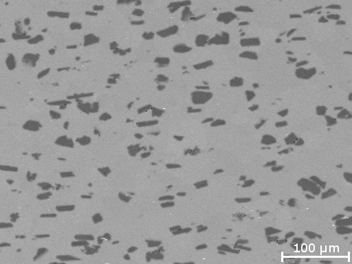
We were faced with this kind of situation when investigating and modelling metal-matrix composites with ceramic particles as reinforcing inclusions (see Figure 1) with respect to their fatigue behaviour. The kind of model intended for the fatigue behaviour (Baaske et al., 2018) is based on a model for the spatial configuration of the ceramic inclusions.

Figure 1: Planar section (cutout) of a metal-matrix composite with reinforcing ceramic particles resulting from scanning electron microscopy.

Besides a model for the spatial arrangement of the inclusions (based on the force-biased algorithm for ellipsoids, see Bezrukov and Stoyan, 2006) this requires the availability of a reasonable model for the distribution of the inclusions in the sense of a grain distribution (Chiu et al., 2013, Sect. 6.5.1). Under the assumption of spatial stationarity it is justified to speak of the typical inclusion, i. e., the distribution of which does not depend on the particular (stationary) spatial arrangement of the inclusions (cf., e. g., Schneider and Weil, 2008, Sect. 4.2); likewise this applies for the distribution of the typical section profile of those inclusions which are intersected by some plane. With this reasoning in mind and since in the present paper we solely focus on the distribution of the typical inclusion we will throughout the paper work with a stationary Poisson particle process (Schneider and Weil, 2008, Sect. 4.1) for the spatial arrangement even when processing the data (where the Poisson assumption is certainly not true), which is an established approach in stereology (Chiu et al., 2013, p. 437).

In particular, due to the possible flexibility w.r.t. shape, we decided to model the typical inclusion as a random ellipsoid with randomness in size, shape and orientation. Thus it is then natural to model the intersected inclusions in the observable planar sections as ellipses for which size, shape and orientation (in the plane) can be estimated from digital images.

Dating back to Wicksell (1926) the respective stereological objective is to infer the joint distribution of the ellipsoids’ size and shape (and also orientation) from the ellipses observable in the planar section which turned out to be solvable completely and uniquely only in case the ellipsoids are all either prolate or oblate spheroids (ellipsoids of revolution), see the pioneering work of Cruz-Orive (1976). The general solution of unfolding the joint size-shape-orientation distribution of the observable ellipses in the plane into the joint size-shape-orientation distribution of the spheroids was given by Beneš et al. (1997) and Beneš and Krejčíř (1997), see also Beneš and Rataj (2004, Ch. 6). Hence, from the empirical 3D joint size-shape-orientation distribution, typically available as a histogram, one may estimate the parameters of a parametric spheroid distribution, for instance by the maximum likelihood method.

A different way is to estimate the parameters based on statistics directly available from the 2D joint size-shape-orientation distribution of the ellipses. A general approach for such a kind of estimation would be to find those model parameters which lead to statistics most similar to the observed ones in the sense of a least squares or minimum contrast approach. Instead of minimizing a distance a related alternative is to find the root of an estimation equation. A particular such estimation equation is based on the so-called quasi-score function which leads to quasi-likelihood estimation, see Heyde (1997) for the general theory. A general problem which holds both for finding a minimum or a root is to explore efficiently the space of possible parameters in case the objective function can be determined only by simulations. For quasi-likelihood estimation an approach is given in Baaske et al. (2014).

The aim of the present paper, motivated by the following facts, is to compare the (possibly more established) way of estimating the parameters by the maximum likelihood method based on the stereologically unfolded joint size-shape-orientation distribution with the quasi-likelihood estimation approach. On the one hand, quasi-likelihood estimation based on simulations is much more involved than unfolding followed by maximum likelihood estimation. On the other hand, unfolding as the solution of an ill-posed inverse problem has a tendency to corrupt the subsequent parameter estimation whereas in quasi-likelihood estimation the available information contained in the employed statistics is used in an optimal way, as demonstrated in Baaske et al. (2014) with an example in a spatial context, leading to more precise estimation results.

The paper is organized as follows. In Section 2 we introduce the parametric model for a spheroid distribution for which we aim to estimate parameters. Furthermore, in Section 3, we first summarize the necessary facts for the trivariate unfolding related to prolate spheroids and give then details for the subsequent maximum likelihood estimation. In Section 4 we sketch the ideas of the quasi-likelihood estimation approach. Then, in Section 5, we compare both approaches by means of a simulation study. Finally, in Section 6 we apply them to a planar section of a system of particles and end up with some conclusions in Section 7.

2 A parametric spheroid distribution

In view of the two basic possibilities of taking the ellipsoids for a reasonable stereological unfolding all either as prolate or as oblate spheroids and respecting findings on the reinforcing particles in a metal-matrix composite (Borbély et al., 2004) quite similar to that in our application in Section 6 we restrict henceforth to prolate spheroids with lengths $a\geq b=c$ of the semi-axes. The shape factor (aspect ratio) $s$ of such a prolate spheroid is then defined as $s=c/a$ and satisfies $0<s\leq 1$. Finally, the orientation of a prolate spheroid as the direction of the axis of revolution can be described in terms of spherical coordinates $(\vartheta,\varphi)$ w.r.t. a fixed axis $u$ with polar angle $\vartheta\in[0,\pi/2)$ and azimuthal angle $\varphi\in[0,2\pi)$. Hence, besides location, a (prolate) spheroid is described for instance by $(a,s,\vartheta,\varphi)$ or $(c,s,\vartheta,\varphi)$, respectively.

To simplify matters we assume that the distribution of the orientations is independent of that of the sizes and shapes. Furthermore, the production process (Müller et al., 2015) of the metal-matrix composite justifies the assumption that the distribution of the system of spheroids is invariant w.r.t. rotations about the fixed axis $u$. One such model for the random orientation of a spheroid respecting this kind of invariance is the ‘Schladitz distribution’ (Franke et al., 2016) which has probability density function (p.d.f.)

$$h_{\beta}(\vartheta,\varphi)=\frac{1}{2\pi}\cdot\frac{1}{2}\frac{\beta\sin\vartheta}{(1+(\beta^{2}-1)\cos^{2}\vartheta)^{\frac{3}{2}}},\quad\vartheta\in[0,\pi),\varphi\in[0,2\pi),$$ (1)

see also Ohser and Schladitz (2009, Eq. (7.11)). In this model $\beta>0$ is an anisotropy parameter in the sense that for decreasing $\beta<1$ the spheroids tend to be more and more parallel to the $u$-axis, and, respectively, for increasing $\beta>1$ the spheroids tend to be more and more parallel to the plane perpendicular to $u$, where $\beta=1$ is the case of isotropically distributed directions.

Since the population of ceramic particles suggests a possible dependence of size and shape of the corresponding representing ellipsoids and a typical size distribution for granular inclusions in materials science is the log-normal distribution, in particular, Borbély et al. (2004) figured out that the log-normal distribution is a good model for the particle sizes in a composite material similar to that considered in Section 6, we aim to work with the following model for the length $a$ of the semi-major axis and the shape factor $s$. Let $(\xi,\eta)$ be a bivariate normally distributed random vector with mean vector $\mu=(\mu_{1},\mu_{2})\in\mathbb{R}^{2}$ and variance-covariance-matrix

$$\Sigma=\begin{pmatrix}\sigma_{1}^{2}&\varrho\sigma_{1}\sigma_{2}\\ \varrho\sigma_{1}\sigma_{2}&\sigma_{2}^{2}\end{pmatrix},\quad\sigma_{1},\sigma_{2}\geq 0,-1\leq\varrho\leq 1.$$ (2)

Then let

$$a=\exp(\xi),\quad s=\frac{1}{1+\exp(-\eta)}.$$ (3)

The parameter $\varrho$ accounts for a possible dependence of size and shape, in particular, $a$ and $s$ are independent if and only if $\varrho=0$. Furthermore, for $\sigma_{1}=0$ or $\sigma_{2}=0$ the cases of a deterministic size or a deterministic shape are included. Note that the approach (3) ensures that the shape factor $s$ is always between $0$ and $1$ and, implying $a>c$, that the corresponding spheroids are always prolate.

All in all we end up with a parametric model for the size-shape-orientation distribution of a random spheroid including the six parameters $(\mu_{1},\mu_{2},\sigma_{1},\sigma_{2},\varrho,\beta)$. If a system of $n$ spheroids (for instance associated with the ceramic inclusions) was observable directly in terms of $(a_{l},s_{l},\vartheta_{l})$, $l=1,\ldots,n$, then the usual way of parameter estimation would be the maximum likelihood method since the likelihood is available. In what follows we discuss two ways how the model parameters might be estimated in case only planar sections of the inclusions are given.

3 Maximum likelihood estimation after trivariate unfolding

3.1 Unfolding

Let $\Psi_{V}$ be a stationary spheroid process with intensity $\lambda_{V}$ which is intersected by a random plane $\mathcal{H}$ with normal direction $v$ perpendicular to the reference direction $u$, i. e. $v$ has polar angle $\pi/2$ and uniformly on $[0,2\pi)$ distributed azimuthal angle ($\overline{\varphi}$) w.r.t. $u$ (termed ‘vertical uniform random section’ in case $u=(0,0,1)$, see Beneš and Rataj, 2004).

Figure 2: Section ellipse of a spheroid within a vertical uniform random section plane.

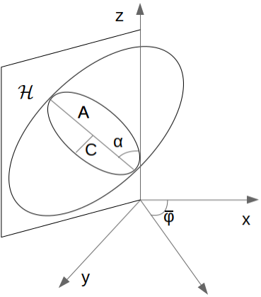
In case a spheroid is hit by $\mathcal{H}$ the intersection of both is an ellipse with lengths $A$ and $C$, $A\geq C$, of the two semi-axes, related shape factor $S=C/A$ and angle $\alpha$ between the semi-major axis and the reference direction $u$, see Figure 2 for an illustration. The cumulative distribution function (c.d.f.) $G(C,S,\alpha)$ of the triple $(C,S,\alpha)$ related to the typical intersection ellipse and the c.d.f. $H(c,s,\vartheta)$ of the triple $(c,s,\vartheta)$ related to the typical spheroid are related to each other by the integral equation

$$\lambda_{A}G(C,S,\alpha)=\frac{4}{\pi}\lambda_{V}\int\mathbf{1}_{[C,\infty)}(c)(c-\sqrt{c^{2}-C^{2}})K_{0}(\alpha,S,\vartheta,s)\,\mathrm{d}H(c,s,\vartheta),$$ (4)

see Beneš and Rataj (2004, Thm. 6.17), where $\lambda_{A}$ is the intensity of the stationary intersection ellipse process and $K_{0}(\alpha,S,\vartheta,s)$ is some function, the explicit form of which is omitted here and can be found in the cited theorem. Based on the observations $(C_{l},S_{l},\alpha_{l})$, $l=1,\ldots,n$, the objective of unfolding is to reconstruct $H(c,s,\vartheta)$ by solving (4) for $H(c,s,\vartheta)$. The numerical solution presented in Beneš and Rataj (2004, Sect. 6.3.3), which we aim to apply in what follows, transforms the integral equation (4) into a system of linear equations by discretization and solves this system with the help of the expectation-maximization algorithm. The discretization is based on classes

$$D_{ijk}=\{(c,s,\vartheta):\,c_{i-1}<c\leq c_{i},s_{j-1}<s\leq s_{j},\vartheta_{k-1}<\vartheta\leq\vartheta_{k}\},$$

$i=1,\ldots,N_{c}$, $j=1,\ldots,N_{s}$, $k=1,\ldots,N_{\vartheta}$, and, respectively,

$$\tilde{D}_{IJK}=\{(C,S,\alpha):\,C_{I-1}<C\leq C_{I},S_{J-1}<S\leq S_{J},\alpha_{K-1}<\alpha\leq\alpha_{K}\},$$

$I=1,\ldots,N_{C}$, $J=1,\ldots,N_{S}$, $K=1,\ldots,N_{\alpha}$, where for simplicity we work with $N_{C}=N_{c}$, $N_{S}=N_{s}$, $N_{\alpha}=N_{\vartheta}$ and $\tilde{D}_{ijk}=D_{ijk}$ for all $(i,j,k)$.

From the planar observations first a normalized trivariate histogram with relative frequencies $g_{ijk}$ related to class $D_{ijk}$ is determined. Then unfolding results in another normalized trivariate histogram with relative frequencies $h_{ijk}$ which is a kind of kernel density estimation of the probability density function of $H(c,s,\vartheta)$.

An implementation of the unfolding procedure as in Beneš and Rataj (2004, Sect. 6.3.3) adapted to the case of prolate spheroids is available within the contributed R package unfoldr, see Baaske (2017).

3.2 Maximum likelihood estimation

Since the result of the unfolding is the trivariate size-shape-orientation histogram $(h_{ijk})$ a subsequent maximum likelihood estimation has to be based on that and not on the original likelihood related to $(c,s,\vartheta)$ or, equivalently, $(a,s,\vartheta)$.

In the model introduced in Section 2 we assume that the orientation of the spheroids is independent of size and shape. Hence the parameter $\beta$ of the orientation distribution can be estimated separately. The respective log-likelihood reads

$$\log\left(L\left((h_{\cdot\cdot k});\beta\right)\right)=\sum_{k=1}^{N_{\vartheta}}h_{\cdot\cdot k}\log\bigg{(}\mathsf{P}_{\!\beta}\big{(}(\vartheta_{k-1},\vartheta_{k}]\big{)}\bigg{)}$$

where $\mathsf{P}_{\!\beta}$ denotes the probability measure related to the p.d.f. $h_{\beta}$,

$$h_{\cdot\cdot k}=\sum_{i=1}^{N_{c}}\sum_{j=1}^{N_{s}}h_{ijk}$$

is the marginal relative frequency in bin $(\vartheta_{k-1},\vartheta_{k}]$, $k=1,\ldots,N_{\vartheta}$, and $N_{c}$, $N_{s}$ and $N_{\vartheta}$ are the numbers of bins for, respectively, $c$, $s$ and $\vartheta$ as in Section 3.1.

Furthermore, with $f_{\mu,\Sigma}$ the p.d.f. of a bivariate normal distribution with mean $\mu=(\mu_{1},\mu_{2})$ and variance-covariance matrix $\Sigma$ as in (2), the joint p.d.f. of the length $c$ of the semi-minor axis and the shape factor $s$ is

$$h_{\mu,\Sigma}(c,s)=\frac{1}{c\,s\,(1-s)}\,f_{\mu,\Sigma}(\log(c/s),\log(s/(1-s)))$$

since the reverse transform of $(\xi,\eta)\mapsto(c,s)=(\exp(\xi)/(1+\exp(-\eta)),1/(1+\exp(-\eta))$ as in (3) is $(c,s)\mapsto(\xi,\eta)=(\log(c/s),\log(s/(1-s))$ with Jacobian $(c\,s\,(1-s))^{-1}$. Then, denoting by $\mathsf{P}_{\!\mu,\Sigma}$ the probability measure related to the p.d.f. $h_{\mu,\Sigma}$, the log-likelihood reads

$$\log\left(L\left((h_{ij\cdot});\mu,\Sigma\right)\right)=\sum_{i=1}^{N_{c}}\sum_{j=1}^{N_{s}}h_{ij\cdot}\log\bigg{(}\mathsf{P}_{\!\mu,\Sigma}\big{(}(c_{i-1},c_{i}]\times(s_{j-1},s_{j}]\big{)}\bigg{)},$$

where

$$h_{ij\cdot}=\sum_{k=1}^{N_{\vartheta}}h_{ijk}$$

is the marginal relative frequency in the class $(c_{i-1},c_{i}]\times(s_{j-1},s_{j}]$, $i=1,\ldots,N_{s}$, $j=1,\ldots,N_{c}$.

4 Quasi-likelihood estimation

The idea of the quasi-likelihood estimation approach which we aim to apply is to estimate the unknown parameter $\theta$ (taking values in an open subset $\Theta$ of the $p$-dimensional Euclidean space $\mathbb{R}^{p}$) by finding a root $\hat{\theta}_{QL}$ of the quasi-score estimating function

$$Q(\theta,y)=\left(\frac{\partial\mathsf{E}_{\theta}[T(X)]}{\partial\theta}\right)^{\!\!\top}\mathsf{Var}_{\theta}[T(X)]^{-1}(y-\mathsf{E}_{\theta}[T(X)]),$$ (5)

where $X$ is a random variable on the sample space $\mathbb{X}$ with distribution $\mathsf{P}_{\!\theta}$, $T\colon\mathbb{X}\to\mathbb{R}^{q}$ is a transformation of $X$ to a vector of summary statistics, $y=T(x)$ is the respective (column) vector of summary statistics for the observed data $x$, $(\cdot)^{\top}$ denotes transpose, and, respectively, $\mathsf{E}_{\theta}$ and $\mathsf{Var}_{\theta}$ denote expectation and variance w.r.t. $\mathsf{P}_{\!\theta}$. For a fixed choice $T$ of summary statistics, the quasi-score estimating function $Q$ in (5) is that standardized estimation function

$$\tilde{G}=-\left(\mathsf{E}_{\theta}\left[\frac{\partial G}{\partial\theta}\right]\right)^{\!\!\top}\left(\mathsf{E}_{\theta}\left[GG^{\top}\right]\right)^{-1}G,$$ (6)

$G(\theta,y)=y-\mathsf{E}_{\theta}(T(X))$, for which the information criterion

$$\mathcal{E}(G)=\mathsf{E}_{\theta}[\tilde{G}\tilde{G}^{\top}]=\left(\mathsf{E}_{\theta}\left[\frac{\partial G}{\partial\theta}\right]\right)^{\!\!\top}\left(\mathsf{E}_{\theta}\left[GG^{\top}\right]\right)^{-1}\left(\mathsf{E}_{\theta}\left[\frac{\partial G}{\partial\theta}\right]\right)$$ (7)

is maximized in the partial order of non-negative definite matrices (Godambe and Heyde, 1987; Heyde, 1997) among all linear standardized unbiased estimating functions of the form $A(\theta)(y-\mathsf{E}_{\theta}(T(X)))$, $A(\theta)$ being any $(p\times q)$-dimensional matrix such that the matrix $A(\theta)\mathsf{Var}_{\theta}[T(X)]A(\theta)^{\top}$ is non-singular.

The information criterion in (7) is a generalization of the well-known Fisher information since it coincides with the Fisher information in case a likelihood is available and $G$ equals the usual score function. Then, in analogy to maximum likelihood estimation, the inverse of $\mathcal{E}(G)$ has a direct interpretation as the asymptotic variance of the estimator $\hat{\theta}_{QL}$. For the quasi-likelihood estimation based on (5) and the particular vector $T$ of summary statistics the information criterion reads

$$I_{T}(\theta)=\mathsf{Var}_{\theta}[Q(\theta,T(X))]=\left(\frac{\partial\mathsf{E}_{\theta}[T(X)]}{\partial\theta}\right)^{\!\!\top}\mathsf{Var}_{\theta}[T(X)]^{-1}\left(\frac{\partial\mathsf{E}_{\theta}[T(X)]}{\partial\theta}\right)$$ (8)

and is called quasi-information matrix in what follows.

Similar to finding a root of the score in maximum likelihood estimation by Fisher scoring, the quasi-score equation (5) can be solved with the Fisher quasi-scoring iteration

$$\theta^{(k+1)}=\theta^{(k)}+t^{(k)}\delta^{(k)},\quad\delta^{(k)}=I_{T}(\theta^{(k)})^{-1}Q(\theta^{(k)},y),$$ (9)

where $t^{(k)}$ is some step length parameter (Osborne, 1992; Baaske et al., 2014), in case the quasi-score $Q$ and the quasi-information matrix $I_{T}$ are available as a closed form expression which can be evaluated at least numerically. In particular, this would include to know expectations and variances of the employed summary statistics $T$ w.r.t. to $\mathrm{P}_{\!\theta}$ as a function of $\theta$. However, in many cases including the setting under investigation these expectations and variances are available only as Monte Carlo estimates based on simulated realizations of the random variable $X$ under $\mathrm{P}_{\!\theta}$. Then, still, (9) might be applied in case simulations are fast and thus the Monte Carlo error can be made small by a sufficiently large number of used model realizations. For more involved simulations, however, a Monte Carlo error cannot be avoided, making a direct application of (9) unreasonable. In Baaske et al. (2014) an idea is presented how the quasi-likelihood estimation approach can be applied even in that case. A respective routine has been developed within the contributed R package qle (Baaske, 2018).

5 Simulation study

The generation of the data for the simulation study includes the following steps. First a realization of a stationary Poisson spheroid process with some fixed intensity $\lambda_{V}$ (below with the concrete value $50$) and with distribution $\mathrm{P}_{\!\theta}$, $\theta=(\mu_{1},\mu_{2},\sigma_{1},\sigma_{2},\varrho,\beta)$, related to the typical (prolate) spheroid (see Section 2) is generated. Since in this model we allow for spheroids which are not almost surely bounded, it is not sufficient to simulate the Poisson spheroid process in an enlarged window in order to avoid edge effects, see Chiu et al. (2013, Sect. 3.1.4). Rather we need an exact simulation method. From the two available general approaches given in Lantuéjoul (2002, Sect. 13.2.1) and Lantuéjoul (2013) the one in the latter reference is appropriate but has to be tailored to our specific model. We postpone the details to the Appendix. Then, all spheroids hitting the planar observation window (taken below as a square of side length $10$) inside the section plane $\mathcal{H}$ are identified and the corresponding intersection ellipses are determined. In the sense of an edge correction only section ellipses are considered which have their centres inside the planar observation window. The simulated data then consists of a random number $n$ of triples $(C_{l},S_{l},\alpha_{l})$, $l\in J=\{1,\ldots,n\}$.

For the unfolding procedure we consider several grades of fineness for binning the ranges of the 2D data. Since binning the data is a particular case of a kernel density estimation the known problem of small biases and large variances for small bin widths as well as large biases and small variances for large bin widths applies, and the optimal bin width minimizing the mean squared error is unknown. The choices for the numbers $(N_{C},N_{S},N_{\alpha})$ of bins, ordered from coarse to fine binning, are

$$(6,5,6),\quad(8,5,8),\quad(12,7,10),\quad(15,10,12),\quad(18,12,15).$$ (10)

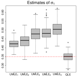
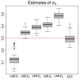
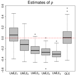
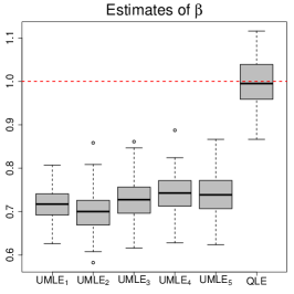
After unfolding the parameters are estimated by maximum likelihood according to the likelihoods given in Section 3.2. These in total five methods are denoted as ‘UMLE₁’, ‘UMLE₂’, ‘UMLE₃’, ‘UMLE₄’ and ‘UMLE₅’ in the order of the grade of fineness for the binning as in (10).

Furthermore, writing ‘med’ for the median, ‘mad’ for the median absolute deviation and ‘cor’ for Pearson’s correlation coefficient, we employ for the quasi-likelihood estimation, denoted by ‘QLE’, the $q=12$ statistics

$$\mathrm{med}\big{(}\{\log(C_{l})\}_{l\in J}\big{)},\;\mathrm{med}\big{(}\{\log(A_{l})\}_{l\in J}\big{)},\;\mathrm{med}\big{(}\{Y_{l}\}_{l\in J}\big{)},\;\mathrm{med}\big{(}\{S_{l}\}_{l\in J}\big{)},\;\mathrm{med}\big{(}\{\alpha_{l}\}_{l\in J}\big{)}$$

$$\mathrm{mad}\big{(}\{\log(C_{l})\}_{l\in J}\big{)},\;\mathrm{mad}\big{(}\{\log(A_{l})\}_{l\in J}\big{)},\;\mathrm{mad}\big{(}\{Y_{l}\}_{l\in J}\big{)},\;\mathrm{mad}\big{(}\{S_{l}\}_{l\in J}\big{)},\;\mathrm{mad}\big{(}\{\alpha_{l}\}_{l\in J}\big{)}$$

$$\mathrm{cor}\big{(}\{\log(C_{l})\}_{l\in J},\{\log(A_{l})\}_{l\in J}\big{)},\;\mathrm{cor}\big{(}\{\log(A_{l})\}_{l\in J},\{Y_{l}\}_{l\in J}\big{)},$$

where $A_{l}=C_{l}/S_{l}$ and $Y_{l}=\log(S_{l}/(1-S_{l}))$, $l\in J$.

In order not only to have a comparison between the six methods applied to the 2D data but to assess somehow the precision of the respective estimates we have considered estimating the parameters from 3D data, that is, for the case that the spheroids were observable directly and not through a planar section. Besides maximum likelihood estimation (denoted by ‘MLE3D’) applied to the 3D data $(c_{l},s_{l},\vartheta_{l})$ we also employ maximum likelihood estimation as in Section 3.2 after binning the 3D data according to the same classification (10) as used for the 2D data, denoting these methods by ‘BINMLE₁’, ‘BINMLE₂’, ‘BINMLE₃’, ‘BINMLE₄’ and ‘BINMLE₅’. Since the latter six methods are based on a different kind of data as the first six methods, each a sub-sample of size $n$ (which is the respective 2D sample size) was taken.

With each 100 repetitions we have considered five different combinations of parameters. In the first setting the parameters were chosen as

$$\mu_{1}=-2.15,\;\mu_{2}=0.55,\;\sigma_{1}=0.35,\;\sigma_{2}=0.3,\;\varrho=0,\;\beta=1,$$

that is, with independent size and shape and isotropic orientation distribution. In the second and third setting all parameters but $\beta$ are kept the same, and the choices $\beta=10$ and $\beta=0.5$ lead to a relatively strong alignment of the spheroids parallel respectively to a plane, or, to a line, see the reasoning in Section 2 around Eq. (1). In the forth and fifth setting all parameters but $\varrho$ are the same as in the first setting, and the choices $\varrho=0.25$ and $\varrho=0.75$, respectively, imply two different levels of dependence between size and shape.

Figure 3: Boxplots of the parameter estimates for original parameters $(\mu_{1},\mu_{2},\sigma_{1},\sigma_{2},\varrho,\beta)=(-2.15,0.55,0.35,0.3,0.0,1.0)$ (indicated by red dashed lines) from 2D sections with unfolding based on five different bin widths followed each by maximum likelihood estimation (UMLE₁,…,UMLE₅) as well as with quasi-likelihood estimation (QLE).

Table 1: Root mean squared error (rmse) of the parameter estimates for original parameters $(\mu_{1},\mu_{2},\sigma_{1},\sigma_{2},\varrho,\beta)=(-2.15,0.55,0.35,0.3,0.0,1.0)$ (top) from 2D sections with unfolding based on five different bin widths followed each by maximum likelihood estimation (UMLE₁,…,UMLE₅) as well as with quasi-likelihood estimation (QLE), and (bottom) from 3D data with maximum likelihood (MLE3D) and with maximum likelihood after classifying the 3D data into the same five binnings as used for unfolding (BINMLE₁,…,BINMLE₅).

Method	rmse$(\hat{\mu}_{1})$	rmse$(\hat{\mu}_{2})$	rmse$(\hat{\sigma}_{1})$	rmse$(\hat{\sigma}_{2})$	rmse$(\hat{\varrho})$	rmse$(\hat{\beta}$)
UMLE1	0.133	0.259	0.077	0.184	0.206	0.285
ULME2	0.096	0.254	0.095	0.052	0.193	0.303
ULME3	0.142	0.080	0.137	0.094	0.247	0.276
ULME4	0.159	0.032	0.142	0.114	0.274	0.262
ULME5	0.195	0.128	0.164	0.187	0.306	0.264
QLE	0.025	0.033	0.027	0.040	0.167	0.053

Method	rmse$(\hat{\mu}_{1})$	rmse$(\hat{\mu}_{2})$	rmse$(\hat{\sigma}_{1})$	rmse$(\hat{\sigma}_{2})$	rmse$(\hat{\varrho})$	rmse$(\hat{\beta}$)
BINMLE1	0.013	0.041	0.012	0.087	0.088	0.036
BINMLE2	0.011	0.011	0.011	0.008	0.032	0.039
BINMLE3	0.013	0.011	0.010	0.008	0.038	0.032
BINMLE4	0.013	0.011	0.008	0.008	0.037	0.034
BINMLE5	0.013	0.010	0.008	0.007	0.035	0.035
MLE3D	0.012	0.011	0.008	0.007	0.035	0.039

Table 2: Root mean squared error (rmse) of the parameter estimates for original parameters $(\mu_{1},\mu_{2},\sigma_{1},\sigma_{2},\varrho,\beta)=(-2.15,0.55,0.35,0.3,0.0,10.0)$ (top) from 2D sections with unfolding based on five different bin widths followed each by maximum likelihood estimation (UMLE₁,…,UMLE₅) as well as with quasi-likelihood estimation (QLE), and (bottom) from 3D data with maximum likelihood (MLE3D) and with maximum likelihood after classifying the 3D data into the same five binnings as used for unfolding (BINMLE₁,…,BINMLE₅).

Method	rmse$(\hat{\mu}_{1})$	rmse$(\hat{\mu}_{2})$	rmse$(\hat{\sigma}_{1})$	rmse$(\hat{\sigma}_{2})$	rmse$(\hat{\varrho})$	rmse$(\hat{\beta}$)
UMLE1	0.119	0.269	0.093	0.203	0.256	6.382
ULME2	0.069	0.298	0.097	0.038	0.182	6.399
ULME3	0.130	0.039	0.127	0.225	0.302	5.972
ULME4	0.145	0.073	0.139	0.255	0.322	5.409
ULME5	0.183	0.233	0.155	0.363	0.353	5.125
QLE	0.039	0.066	0.031	0.050	0.284	0.459

Method	rmse$(\hat{\mu}_{1})$	rmse$(\hat{\mu}_{2})$	rmse$(\hat{\sigma}_{1})$	rmse$(\hat{\sigma}_{2})$	rmse$(\hat{\varrho})$	rmse$(\hat{\beta}$)
BINMLE1	0.012	0.032	0.014	0.062	0.065	0.792
BINMLE2	0.013	0.011	0.010	0.008	0.037	0.707
BINMLE3	0.011	0.009	0.009	0.007	0.035	0.641
BINMLE4	0.010	0.011	0.008	0.008	0.040	0.488
BINMLE5	0.013	0.009	0.008	0.007	0.032	0.434
MLE3D	0.010	0.009	0.007	0.006	0.033	0.370

Table 3: Root mean squared error (rmse) of the parameter estimates for original parameters $(\mu_{1},\mu_{2},\sigma_{1},\sigma_{2},\varrho,\beta)=(-2.15,0.55,0.35,0.3,0.0,0.5)$ (top) from 2D sections with unfolding based on five different bin widths followed each by maximum likelihood estimation (UMLE₁,…,UMLE₅) as well as with quasi-likelihood estimation (QLE), and (bottom) from 3D data with maximum likelihood (MLE3D) and with maximum likelihood after classifying the 3D data into the same five binnings as used for unfolding (BINMLE₁,…,BINMLE₅).

Method	rmse$(\hat{\mu}_{1})$	rmse$(\hat{\mu}_{2})$	rmse$(\hat{\sigma}_{1})$	rmse$(\hat{\sigma}_{2})$	rmse$(\hat{\varrho})$	rmse$(\hat{\beta}$)
UMLE1	0.114	0.287	0.08	0.186	0.197	0.106
ULME2	0.078	0.306	0.097	0.029	0.182	0.131
ULME3	0.114	0.150	0.137	0.074	0.257	0.124
ULME4	0.137	0.077	0.148	0.090	0.272	0.121
ULME5	0.168	0.046	0.162	0.147	0.293	0.123
QLE	0.027	0.032	0.026	0.034	0.163	0.027

Method	rmse$(\hat{\mu}_{1})$	rmse$(\hat{\mu}_{2})$	rmse$(\hat{\sigma}_{1})$	rmse$(\hat{\sigma}_{2})$	rmse$(\hat{\varrho})$	rmse$(\hat{\beta}$)
BINMLE1	0.015	0.048	0.012	0.101	0.097	0.018
BINMLE2	0.012	0.013	0.011	0.010	0.039	0.019
BINMLE3	0.011	0.011	0.010	0.009	0.037	0.019
BINMLE4	0.012	0.011	0.011	0.008	0.038	0.017
BINMLE5	0.011	0.010	0.010	0.007	0.035	0.017
MLE3D	0.011	0.010	0.009	0.007	0.035	0.017

Table 4: Root mean squared error (rmse) of the parameter estimates for original parameters $(\mu_{1},\mu_{2},\sigma_{1},\sigma_{2},\varrho,\beta)=(-2.15,0.55,0.35,0.3,0.25,1.0)$ from 2D sections with unfolding based on five different bin widths followed each by maximum likelihood estimation (UMLE₁,…,UMLE₅) as well as with quasi-likelihood estimation (QLE).

Method	rmse$(\hat{\mu}_{1})$	rmse$(\hat{\mu}_{2})$	rmse$(\hat{\sigma}_{1})$	rmse$(\hat{\sigma}_{2})$	rmse$(\hat{\varrho})$	rmse$(\hat{\beta}$)
UMLE1	0.160	0.239	0.083	0.202	0.224	0.285
ULME2	0.121	0.231	0.098	0.051	0.262	0.302
ULME3	0.161	0.069	0.148	0.094	0.406	0.277
ULME4	0.179	0.040	0.155	0.108	0.431	0.268
ULME5	0.211	0.142	0.175	0.185	0.485	0.264
QLE	0.031	0.047	0.032	0.046	0.258	0.050

Table 5: Root mean squared error (rmse) of the parameter estimates for original parameters $(\mu_{1},\mu_{2},\sigma_{1},\sigma_{2},\varrho,\beta)=(-2.15,0.55,0.35,0.3,0.75,1.0)$ from 2D sections with unfolding based on five different bin widths followed each by maximum likelihood estimation (UMLE₁,…,UMLE₅) as well as with quasi-likelihood estimation (QLE).

Method	rmse$(\hat{\mu}_{1})$	rmse$(\hat{\mu}_{2})$	rmse$(\hat{\sigma}_{1})$	rmse$(\hat{\sigma}_{2})$	rmse$(\hat{\varrho})$	rmse$(\hat{\beta}$)
UMLE1	0.217	0.188	0.081	0.242	0.225	0.287
ULME2	0.171	0.174	0.104	0.049	0.444	0.291
ULME3	0.195	0.041	0.148	0.084	0.685	0.281
ULME4	0.214	0.072	0.158	0.106	0.716	0.273
ULME5	0.240	0.179	0.178	0.176	0.786	0.272
QLE	0.034	0.050	0.044	0.084	0.266	0.066

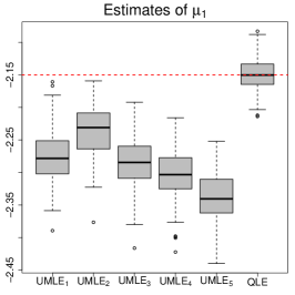
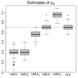
The results of the simulation study for the first choice $(-2.15,0.55,0.35,0.3,0.0,1.0)$ of parameters, given in Figure 3 in terms of boxplots and in Table 1 in terms of root mean squared errors (corresponding bootstrap standard errors are given in Table 7) show that QLE provides clearly smaller mean squared errors than most of those from UMLE₁,…,UMLE₅, and that the reason for this behaviour is most of all due to the bias resulting from unfolding. The comparison with the maximum likelihood estimates from the 3D data shows that the effect of binning the data into classes is small whatever the grade of fineness is. Likewise the precision of QLE is roughly (only) one order of magnitude worse than that of MLE3D but one order of magnitude better than that of UMLE₁,…,UMLE₅. Figure 3 shows that a particular choice of bins leads for a certain parameter to a precision comparable to that of QLE whereas with the same choice of bins estimation of another parameter implies a certain bias. These findings also hold for other choices of the parameters, see the root mean squared errors in the Tables 2–5 together with the respective bootstrap standard errors in Tables 8–11 (postponed to the Appendix). In particular, it becomes obvious from Table 2 that the error of the estimates of $\beta=10$ from UMLE₁,…,UMLE₅ is almost as large as the parameter. However, in either case QLE as well as UMLE₁,…,UMLE₅ produce large errors when estimating the parameter $\varrho$, which is not the case when using 3D data, see Tables 1 to 3.

6 Application

We consider an aluminium matrix composite (see Figure 1) reinforced with alumina particles (Al₂O₃, ca. 15% volume fraction), denoted by AA6061-15p, as in Müller et al. (2015) where experimental investigations most of all on the very high cycle fatigue behaviour are performed and further details may be found. Due to extrusion moulding into a bar the particles in AA6061-15p were aligned nearly parallel to the extrusion direction. Therefore, the production process justifies the assumption that the orientation distribution of the reinforcements is invariant with respect to rotations about some fixed axis.

The ceramic inclusions are modelled as prolate spheroids. Although the investigation of a similar sample of ceramic inclusions in Borbély et al. (2004) indicates that a modelling with general ellipses could be even better, prolate spheroids seem to be still sufficiently flexible for the particles and make corresponding planar section data accessible for stereological unfolding in the above sense (Section 3.1). In order to extract the data for the corresponding ellipses from the planar section the 2D image has been segmented and ellipses have been fitted with the help of an image analyser (Pau et al., 2010); the ellipses data is available as the dataset data15p within the R package unfoldr (Baaske, 2017). The aim is to estimate the parameters of the supposed spheroid distribution (see Section 2) from the 2D data with the quasi-likelihood approach. A section plane parallel to the extrusion direction (see Figure 1, left) was used which corresponds to a vertical uniform random section as needed for unfolding (see Section 3.1).

In order to estimate the statistics (see Section 5) needed for QLE an edge correction in the sense of minus-sampling (Chiu et al., 2013, p. 254) has been applied. The results of QLE are given in Table 6, together with the asymptotic standard errors of these estimates as the entries of $\sqrt{\operatorname{diag}(I(\hat{\theta}_{QL})^{-1})}$, cf. Section 4 and Baaske et al. (2014).

Table 6: Estimates and asymptotic standard errors after applying QLE to the AA6061-15p data.

parameter	$\mu_{1}$	$\mu_{2}$	$\sigma_{1}$	$\sigma_{2}$	$\varrho$	$\beta$
estimate	$-3.706$	$-0.782$	$0.358$	$0.567$	$-0.218$	$0.194$
standard error	$0.041$	$0.050$	$0.052$	$0.043$	$0.122$	$0.011$

In order to assess the goodness-of-fit of the QLE parameter estimates we performed each a Kolmogorov-Smirnov test for the length $A$ of the semi-major axis, the length $C$ of the semi-minor axis, the shape factor $S$ and the direction angle $\alpha$ of the section ellipses. The corresponding $p$-values are

$$p_{A}=0.071,\;p_{C}=0.095,\;p_{S}=0.070,\;p_{\alpha}=0.114\,,$$

indicating that the fitted model indeed reflects well the marginal distributions of the essential 2D quantities.

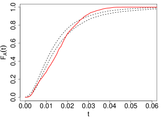
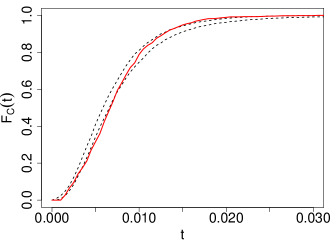
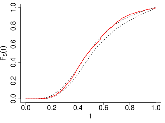
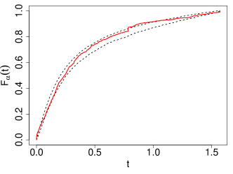
Furthermore, we generated each 199 samples of a Poisson spheroid system such that the mean number of spheroids hitting the observation window equals the sample size of the data. From the data and from the simulated samples each the empirical c.d.f. of the length $A$ of the semi-major axis, of the length $C$ of the semi-minor axis, of the shape factor $S$ and of the direction angle $\alpha$ of the intersection ellipses were determined. In Figure 4 the pointwise 95% envelopes of the empirical c.d.f.s from the simulated samples as well as the corresponding empirical c.d.f. of the data are plotted.

Figure 4: Empirical c.d.f. for the AA6061-15p data (red) and pointwise 95% envelopes of the c.d.f. for the model fitted with quasi-likelihood (black dashed) of length $A$ of the semi-major axis ($F_{A}$, top left), of length $C$ of the semi-minor axis ($F_{C}$, top right), of shape factor $S$ ($F_{S}$, bottom left) and of angle $\alpha$ ($F_{\alpha}$, bottom right).

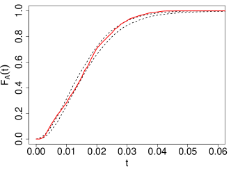
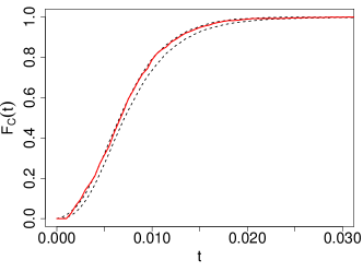
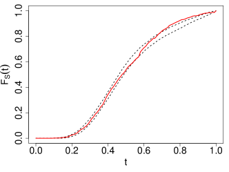
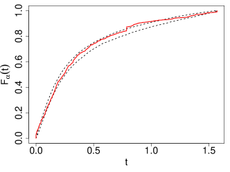
The small jumps in Figure 4 (bottom right) in the empirical c.d.f. $F_{\alpha}$ w.r.t. to the angle $\alpha$ at 0, $\pi/4$ and $\pi/2$ are clearly due to digitisation. All in all it seems that the QLE fit of the spheroid distribution for AA6061-15p can be considered as satisfying.

Although the simulation study in Section 5 indicates that QLE typically outperforms ULME we also fitted the model with maximum likelihood after unfolding. Among UMLE₁,…,UMLE₅ the variant UMLE₄ performs best and results in the following parameter estimates:

$$\hat{\mu}_{1}=-4.030,\;\hat{\mu}_{2}=-0.584,\;\hat{\sigma}_{1}=0.637,\;\hat{\sigma}_{2}=0.677,\;\hat{\varrho}=-0.531,\;\hat{\beta}=0.194$$

Interestingly, the estimated value of $\beta$ is approximately the same with both methods while there is a clear difference for the other parameter estimates. The Kolmogorov-Smirnov test for $A$, $C$, $S$ and $\alpha$ results in the $p$-values

$$p_{A}=0.00001,\;p_{C}=0.00016,\;p_{S}=0.04534,\;p_{\alpha}=0.20664\,,$$

such that, even after correcting for multiple comparisons, the model obtained with UMLE₄ has to be rejected (cf. also Figure 5).

Figure 5: Empirical c.d.f. for the AA6061-15p data (red) and pointwise 95% envelopes of the c.d.f. for the model fitted with maximum likelihood after unfolding (black dashed) of length $A$ of the semi-major axis ($F_{A}$, top left), of length $C$ of the semi-minor axis ($F_{C}$, top right), of shape factor $S$ ($F_{S}$, bottom left) and of angle $\alpha$ ($F_{\alpha}$, bottom right).

7 Conclusions

We have demonstrated the potential of the quasi-likelihood estimation approach for inferring the parameters of a distribution of three-dimensional objects which are observable only through two-dimensional sections, even in the more complicated situation that objective functions are only available as Monte Carlo approximations. Although for certain bin widths of the histograms the precision of the parameter estimates with the maximum likelihood method after the well-known procedure of unfolding is comparable to the precision of the quasi-likelihood estimates the respective bin widths are not known in advance and, more seriously, in general differ for the different parameters. At least in the case of a parametric modelling approach the quasi-likelihood estimation approach should thus be considered as a valuable alternative. For a non-parametric modelling approach, however, unfolding will keep indispensable.

The presented study also strongly supports the so-called ‘two-step method’ as recommended in Chiu et al. (2013, p. 433) for parametric inference based on sectional data, namely first to get ideas on the type of distributions in, say, 3D from a rough solution of the unfolding problem and then to apply a parametric approach involving only the sectional data.

Although the employed parametric model for the random prolate spheroids is of course a particular one, the two investigated methods of parameter estimation might be adapted to other models. We would then expect a similar behaviour w.r.t. the precision of the parameter estimates. Nevertheless, the simulation-based quasi-likelihood estimation approach as implemented in Baaske (2018) is basically applicable in very general settings and thus a powerful tool for parameter estimation in spatial statistics.

For the real-world sample in Section 6 it turns out that the particular parametric spheroid model obtained with the quasi-likelihood approach is able to model the distribution of the ceramic particles in AA6061-15p reasonable well. In particular, the goodness-of-fit test results indicate that the restriction to spheroids, i. e. ellipsoids of revolution, as the shape model for the ceramic inclusions is sufficient. Hence, the fitted model can then be further used, most of all for generating virtual particle configurations for assessing the very high cycle fatigue behaviour of metal-matrix composites as in Baaske et al. (2018).

Appendix A Exact simulation

Since for a prolate spheroid the length of the semi-major axis equals the radius of the smallest circumscribed ball the distribution of this radius is directly given which makes the following exact simulation method quite efficient. An implementation for spheroids is also part of the contributed R package unfoldr, see Baaske (2017).

Denoting by $B_{r}(x)$ a ball in $\mathbb{R}^{3}$ with centre $x\in\mathbb{R}^{3}$ and radius $r\in[0,\infty)$ let $[W]=\{(x,r)\in\mathbb{R}^{3}\times[0,\infty):\,B_{r}(x)\cap W\neq\varnothing\}$ for some convex compact set $W\subset\mathbb{R}^{3}$. Let $\Psi$ be a marked point process on $\mathbb{R}^{3}\times[0,\infty)$ representing a stationary Poisson ball process (Schneider and Weil, 2008, Sect. 4.1) with intensity $\lambda$ and p.d.f. $f_{R}$ (with finite third moment) of the balls’ radii. Then the mean number of balls from $\Psi$ hitting $W$ equals

$$\Lambda_{\Psi}([W]) =\int_{\mathbb{R}^{3}}\int_{0}^{\infty}\!\!\!\lambda\,f_{R}(r)\,\mathbf{1}_{[W]}(x,r)\,\operatorname{d}\!r\operatorname{d}\!x=\int_{\mathbb{R}^{3}}\int_{0}^{\infty}\!\!\!\lambda\,f_{R}(r)\,\mathbf{1}_{W\oplus B_{r}(o)}(x)\,\operatorname{d}\!r\operatorname{d}\!x$$

$$=\int_{0}^{\infty}\!\!\!\!\lambda\,f_{R}(r)\,V(W\oplus B_{r}(o))\,\operatorname{d}\!r=\int_{0}^{\infty}\!\!\!\!\lambda\,f_{R}(r)\,\sum_{k=0}^{3}a_{k}r^{k}\,\operatorname{d}\!r=\lambda\sum_{k=0}^{3}a_{k}\mathsf{E}[R^{k}],$$

where $W\oplus B_{r}(o)=\{x+y:\,x\in W,y\in B_{r}(o)\}$ and $R$ denotes the random ball radius, and where we have used first Fubini’s theorem and then Steiner’s formula; the latter implying $a_{0}=V(W)$, $a_{1}=S(W)$ (the surface area of $W$), $a_{2}=M(W)$ (the integral of mean curvature of $W$) and $a_{3}=4\pi/3$, see Chiu et al. (2013, p. 15f.) and Schneider and Weil (2008, p. 600ff.).

Hence, $\Psi([W])$ follows a Poisson distribution with mean $\lambda\sum_{k=0}^{3}a_{k}\mathsf{E}[R^{k}]$. Given $\Psi([W])=n$ the corresponding $n$ points $(x_{1},r_{1}),\ldots,(x_{n},r_{n})$ from $\Psi$ are i.i.d. according to $\Lambda_{\Psi}(\cdot)/\Lambda_{\Psi}([W])$, i. e. with joint p.d.f.

$$f^{[W]}(x,r)=\frac{\lambda\,f_{R}(r)\,\mathbf{1}_{W\oplus B_{r}(o)}(x)}{\Lambda_{\Psi}([W])},$$

see also Lantuéjoul (2002, Prop. 13.2.1) and Lantuéjoul (2013). This implies that the radii $r_{1},\ldots,r_{n}$ are distributed according to the p.d.f.

$$f^{[W]}(r)=\int_{\mathbb{R}^{3}}f^{[W]}(x,r)\,\mathrm{d}x=\frac{\lambda\,f_{R}(r)\,V(W\oplus B_{r}(o))}{\Lambda_{\Psi}([W])}=\sum_{k=0}^{3}\frac{a_{k}r^{k}f_{R}(r)}{\sum_{j=0}^{3}a_{j}\mathsf{E}[R^{j}]}$$

and, given the radius $r$, the centre $x$ is uniformly distributed on $W\oplus B_{r}(o)$,

$$f^{[W]}(x|r)=\frac{f^{[W]}(x,r)}{f^{[W]}(r)}=\frac{\mathbf{1}_{W\oplus B_{r}(o)}(x)}{V(W\oplus B_{r}(o))}.$$

Hence, for the exact simulation of a stationary Poisson ball process w.r.t. the window $W$, the following algorithm (Algorithm 1 in Lantuéjoul, 2013) is suitable:

Algorithm 1.

• Generate $n$ according to the Poisson distribution with mean $\Lambda_{\Psi}([W])$.

• Generate $r_{1},\ldots,r_{n}$ i.i.d. according to $f^{[W]}(r)$.

• Generate $x_{1},\ldots,x_{n}$ independently and, each conditionally on $r_{i}$, uniformly on $W\oplus B_{r_{i}}(o)$, $i=1,\ldots,n$.

In the most crucial step 2 in Algorithm 1 the distribution is a mixture, i. e. in terms of the respective c.d.f. $F^{[W]}(r)$ we have

$$F^{[W]}(r)=\sum_{k=0}^{3}\frac{a_{k}\mathsf{E}[R^{k};R\leq r]}{\sum_{j=0}^{3}a_{j}\mathsf{E}[R^{j}]}=\sum_{k=0}^{3}\frac{a_{k}\mathsf{E}[R^{k}]}{\sum_{j=0}^{3}a_{j}\mathsf{E}[R^{j}]}\,\frac{\mathsf{E}[R^{k};R\leq r]}{\mathsf{E}[R^{k}]}$$

with mixing weights

$$p_{k}=\frac{a_{k}\mathsf{E}[R^{k}]}{\sum_{j=0}^{3}a_{j}\mathsf{E}[R^{j}]}.$$

Since the random ball radius $R$ has a log-normal distribution $\mathsf{logN}(\mu,\sigma^{2})$, i. e.

$$f_{R}(r)=\frac{1}{\sqrt{2\pi}\sigma\,r}\exp\left(-\frac{(\log(r)-\mu)^{2}}{2\sigma^{2}}\right),$$

where $\mu\in\mathbb{R}$ and $\sigma>0$, we have – as a somewhat nice fact – that for all $k=0,1,\ldots$

$$\frac{\mathsf{E}[R^{k};R\leq r]}{\mathsf{E}[R^{k}]}=\Phi\left(\frac{\log(r)-(\mu+k\sigma^{2})}{\sigma}\right)$$

(where $\Phi$ denotes the c.d.f. of the standard normal distribution) is the c.d.f. of a log-normal distribution $\mathsf{logN}(\mu+k\sigma^{2},\sigma^{2})$. Likewise we have $\mathsf{E}[R^{k}]=\exp(k\mu+k^{2}\sigma^{2}/2)$, $k=0,1,2,3$. Hence, in order to generate random numbers according to $f^{[W]}(r)$ we can apply the following algorithm (similar to Algorithm 2 in Lantuéjoul, 2013):

Algorithm 2.

• Generate a random integer $k$ from $\{0,1,2,3\}$ according to the probabilities

  $$p_{k}=\frac{a_{k}\exp(k\mu+k^{2}\sigma^{2}/2)}{\sum_{j=0}^{3}a_{j}\exp(j\mu+j^{2}\sigma^{2}/2)}.$$

• Deliver a random number from a $\mathsf{logN}(\mu+k\sigma^{2},\sigma^{2})$-distribution.

Once all circumscribed balls hitting $W$ are generated, subsequently the shapes and orientations (see B) of the prolate spheroids can be generated. In case one is interested only in a configuration of spheroids hitting $W$ then possibly a few non-hitting spheroids have to be deleted from the configuration as the final step.

Appendix B Simulation of orientations

From (1) we have

$$h_{\beta}(\vartheta)=\frac{1}{2}\frac{\beta\sin\vartheta}{(1+(\beta^{2}-1)\cos^{2}\vartheta)^{\frac{3}{2}}},\quad\vartheta\in[0,\pi),$$ (11)

and

$$H_{\beta}(\vartheta)=\frac{1}{2}\left(1-\frac{\beta\cos\vartheta}{(1+(\beta^{2}-1)\cos^{2}\vartheta)^{\frac{1}{2}}}\right),\quad\vartheta\in[0,\pi),$$ (12)

for, respectively, the p.d.f. and the c.d.f. of the polar angle $\vartheta$. This in turn leads to the quantile function

$$H_{\beta}^{-1}(q)=\arccos\left(\frac{1-2q}{\sqrt{\beta^{2}-(1-2q)^{2}(\beta^{2}-1)}}\right)$$ (13)

which can be used to generate random numbers according to $H_{\beta}$ with the inversion method.

Appendix C Bootstrap standard errors

In Tables 7–11 the bootstrap standard errors of the estimated root mean squared errors given in Tables 1–5 are provided.

Table 7: Bootstrap standard errors of the estimated root mean squared errors in Table 1.

Method	rmse$(\hat{\mu}_{1})$	rmse$(\hat{\mu}_{2})$	rmse$(\hat{\sigma}_{1})$	rmse$(\hat{\sigma}_{2})$	rmse$(\hat{\varrho})$	rmse$(\hat{\beta}$)
UMLE1	0.0040	0.0053	0.0025	0.0042	0.0127	0.0038
ULME2	0.0042	0.0036	0.0035	0.0022	0.0124	0.0044
ULME3	0.0041	0.0035	0.0043	0.0026	0.0090	0.0046
ULME4	0.0041	0.0029	0.0046	0.0024	0.0093	0.0044
ULME5	0.0039	0.0031	0.0045	0.0028	0.007	0.0045
QLE	0.0019	0.0028	0.0020	0.0028	0.0143	0.0031
BINMLE1	0.0008	0.0032	0.0009	0.0080	0.0068	0.0022
BINMLE2	0.0007	0.0009	0.0008	0.0006	0.0019	0.0029
BINMLE3	0.0009	0.0006	0.0006	0.0006	0.0027	0.0022
BINMLE4	0.0008	0.0008	0.0006	0.0007	0.0021	0.0023
BINMLE5	0.0008	0.0007	0.0005	0.0006	0.0022	0.0027
MLE3D	0.0008	0.0007	0.0006	0.0004	0.0032	0.0031

Table 8: Bootstrap standard errors of the estimated root mean squared errors in Table 2.

Method	rmse$(\hat{\mu}_{1})$	rmse$(\hat{\mu}_{2})$	rmse$(\hat{\sigma}_{1})$	rmse$(\hat{\sigma}_{2})$	rmse$(\hat{\varrho})$	rmse$(\hat{\beta}$)
UMLE1	0.0036	0.0086	0.0024	0.0041	0.0201	0.0189
ULME2	0.0037	0.0033	0.0036	0.0021	0.0104	0.0181
ULME3	0.0044	0.0022	0.0048	0.0025	0.0093	0.0197
ULME4	0.0047	0.0041	0.0063	0.0027	0.0079	0.0214
ULME5	0.0045	0.0039	0.0056	0.0028	0.0071	0.0223
QLE	0.0027	0.0043	0.0020	0.0032	0.0242	0.0340
BINMLE1	0.0008	0.0029	0.0009	0.0072	0.0056	0.0519
BINMLE2	0.0008	0.0010	0.0006	0.0006	0.0024	0.0420
BINMLE3	0.0007	0.0007	0.0006	0.0005	0.0021	0.0465
BINMLE4	0.0007	0.0008	0.0005	0.0006	0.0024	0.0317
BINMLE5	0.0011	0.0007	0.0005	0.0005	0.0024	0.0241
MLE3D	0.0006	0.0006	0.0005	0.0004	0.0020	0.0266

Table 9: Bootstrap standard errors of the estimated root mean squared errors in Table 3.

Method	rmse$(\hat{\mu}_{1})$	rmse$(\hat{\mu}_{2})$	rmse$(\hat{\sigma}_{1})$	rmse$(\hat{\sigma}_{2})$	rmse$(\hat{\varrho})$	rmse$(\hat{\beta}$)
UMLE1	0.0039	0.0085	0.0027	0.0053	0.0148	0.0025
ULME2	0.0037	0.0034	0.0036	0.0019	0.0096	0.0022
ULME3	0.0034	0.0031	0.0045	0.0022	0.0085	0.0024
ULME4	0.0039	0.0031	0.0047	0.0024	0.0081	0.0024
ULME5	0.0042	0.0029	0.0060	0.0027	0.0069	0.0023
QLE	0.0021	0.0021	0.0017	0.0022	0.0134	0.0018
BINMLE1	0.0011	0.0035	0.0009	0.0086	0.0076	0.0012
BINMLE2	0.0009	0.0008	0.0008	0.0007	0.0031	0.0014
BINMLE3	0.0007	0.0007	0.0006	0.0005	0.0026	0.0014
BINMLE4	0.0009	0.0010	0.0009	0.0005	0.0027	0.0014
BINMLE5	0.0007	0.0008	0.0006	0.0005	0.0022	0.0011
MLE3D	0.0008	0.0007	0.0006	0.0005	0.0027	0.0010

Table 10: Bootstrap standard errors of the estimated root mean squared errors in Table 4.

Method	rmse$(\hat{\mu}_{1})$	rmse$(\hat{\mu}_{2})$	rmse$(\hat{\sigma}_{1})$	rmse$(\hat{\sigma}_{2})$	rmse$(\hat{\varrho})$	rmse$(\hat{\beta}$)
UMLE1	0.0042	0.0055	0.0028	0.0044	0.0141	0.0039
ULME2	0.0036	0.0044	0.0037	0.0019	0.0158	0.0042
ULME3	0.0036	0.0044	0.0040	0.0031	0.0115	0.0042
ULME4	0.0038	0.0024	0.0042	0.0024	0.0109	0.0039
ULME5	0.0034	0.0037	0.0043	0.0027	0.0093	0.0039
QLE	0.0023	0.0038	0.0023	0.0035	0.0201	0.0029

Table 11: Bootstrap standard errors of the estimated root mean squared errors in Table 5.

Method	rmse$(\hat{\mu}_{1})$	rmse$(\hat{\mu}_{2})$	rmse$(\hat{\sigma}_{1})$	rmse$(\hat{\sigma}_{2})$	rmse$(\hat{\varrho})$	rmse$(\hat{\beta}$)
UMLE1	0.0041	0.0058	0.0029	0.0037	0.0114	0.0043
ULME2	0.0043	0.0055	0.0033	0.0019	0.0199	0.0048
ULME3	0.0040	0.0027	0.0042	0.0024	0.0134	0.0044
ULME4	0.0038	0.0035	0.0044	0.0023	0.0123	0.0046
ULME5	0.0034	0.0037	0.0043	0.0027	0.0109	0.0044
QLE	0.0058	0.0043	0.0135	0.0285	0.0420	0.0058

References

- Baaske (2017) Baaske, M., 2017. unfoldr: Stereological Unfolding for Spheroidal Particles. R package version 0.6.1, http://cran.r-project.org/package=unfoldr.
- Baaske (2018) Baaske, M., 2018. qle: Simulation-Based Quasi-Likelihood Estimation. R package version 0.17, http://cran.r-project.org/package=qle.
- Baaske et al. (2014) Baaske, M., Ballani, F., van den Boogaart, K. G., 2014. A quasi-likelihood approach to parameter estimation for simulatable statistical models. Image Anal. Stereol. 33, 107–119.
- Baaske et al. (2018) Baaske, M., Illgen, A., Weidner, A., Biermann, H., Ballani, F., 2018. Influence of ceramic particle and fibre reinforcement in metal matrix composites on the VHCF behaviour. Part II: Stochastic modelling and statistical inference. In: Christ, H.-J. (Ed.), Fatigue of Materials at Very High Numbers of Loading Cycles. Experimental Techniques - Mechanisms - Modeling and Fatigue Assessment. Springer, Heidelberg.
- Beneš et al. (1997) Beneš, V., Jiruše, M., Slámová, M., 1997. Stereological unfolding of the trivariate size-shape-orientation distribution of spheroidal particles with application. Acta Materialia 45, 1105–1113.
- Beneš and Krejčíř (1997) Beneš, V., Krejčíř, P., 1997. Decomposition in stereological unfolding problems. Kybernetika 33, 245–258.
- Beneš and Rataj (2004) Beneš, V., Rataj, J., 2004. Stochastic Geometry: Selected Topics. Kluwer, Boston.
- Bezrukov and Stoyan (2006) Bezrukov, A., Stoyan, D., 2006. Simulation and statistical analysis of random packings of ellipsoids. Part. Part. Systems Char. 23, 388–398.
- Borbély et al. (2004) Borbély, A., Csikor, F. F., Zabler, S., Cloetens, P., Biermann, H., 2004. Three-dimensional characterization of the microstructure of a metal matrix composite by holotomography. Materials Science and Engineering A 367, 40–50.
- Chiu et al. (2013) Chiu, S. N., Stoyan, D., Kendall, W. S., Mecke, J., 2013. Stochastic Geometry and its Applications, 3rd Edition. J. Wiley & Sons, Chichester.
- Cruz-Orive (1976) Cruz-Orive, L. M., 1976. Particle size-shape distributions: the general spheroid problem. J. Microscopy 107, 235–253.
- Franke et al. (2016) Franke, J., Redenbach, C., Zhang, N., 2016. On a mixture model for directional data on the sphere. Scand. J. Statist. 43 (1), 139–155.
- Godambe and Heyde (1987) Godambe, V. P., Heyde, C. C., 1987. Quasi-likelihood and optimal estimation. International Statistical Revue 55, 231–244.
- Heyde (1997) Heyde, C. C., 1997. Quasi-Likelihood and Its Applications: A General Approach to Optimal Parameter Estimation. Springer, New York.
- Lantuéjoul (2002) Lantuéjoul, C., 2002. Geostatistical Simulation. Springer, Berlin.
- Lantuéjoul (2013) Lantuéjoul, C., 2013. Exact simulation of a Boolean model. Image Anal. Stereol. 32, 101–105.
- Müller et al. (2015) Müller, A., Weidner, A., Biermann, H., 2015. Influence of reinforcement geometry on the very high-cycle fatigue behavior of aluminum-matrix-composites. Materials Science Forum 825/826, 150–157.
- Nagel (2010) Nagel, W., 2010. Stereology. In: Kendall, W. S., Molchanov, I. (Eds.), New perspectives in stochastic geometry. Oxford University Press, Oxford, pp. 451–475.
- Ohser and Mücklich (2000) Ohser, J., Mücklich, F., 2000. Statistical Analysis of Microstructures in Materials Science. J. Wiley & Sons, Chichester.
- Ohser and Schladitz (2009) Ohser, J., Schladitz, K., 2009. 3D Images of Material Structures. Wiley-VCH, Weinheim.
- Osborne (1992) Osborne, M. R., 1992. Fisher’s method of scoring. Int. Stat. Rev. 60, 99–117.
- Pau et al. (2010) Pau, G., Fuchs, F., Sklyar, O., Boutros, M., Huber, W., 2010. EBImage an R package for image processing with applications to cellular phenotypes. Bioinformatics 26 (7), 979–981.
- Schneider and Weil (2008) Schneider, R., Weil, W., 2008. Stochastic and Integral Geometry. Springer, Berlin.
- Wicksell (1926) Wicksell, S. D., 1926. The corpuscle problem. II: Case of ellipsoidal corpuscles. Biometrika 18, 151–172.