PixelNet: Towards a General Pixel-Level Architecture
Abstract
††* indicates equal contribution; first two authors listed in alphabetical order.We explore architectures for general pixel-level prediction problems, from low-level edge detection to mid-level surface normal estimation [4] to high-level semantic segmentation. Convolutional predictors, such as the fully-convolutional network (FCN), have achieved remarkable success by exploiting the spatial redundancy of neighboring pixels through convolutional processing. Though computationally efficient, we point out that such approaches are not statistically efficient during learning precisely because spatial redundancy limits the information learned from neighboring pixels. We demonstrate that (1) stratified sampling allows us to add diversity during batch updates and (2) sampled multi-scale features allow us to explore more nonlinear predictors (multiple fully-connected layers followed by ReLU) that improve overall accuracy. Finally, our objective is to show how a architecture can get performance better than (or comparable to) the architectures designed for a particular task. Interestingly, our single architecture produces state-of-the-art results for semantic segmentation on PASCAL-Context, surface normal estimation [4] on NYUDv2 dataset, and edge detection on BSDS without contextual post-processing.
1 Introduction
Simplicity is the ultimate sophistication.
Leonardo da Vinci
A surprising number of computer vision problems can be formulated as a dense pixel-wise prediction problem. These include low-level tasks such as edge detection [16, 50, 71] and optical flow [3, 18], mid-level tasks such as depth/normal recovery [4, 19, 20, 60, 68], and high-level tasks such as keypoint prediction [28, 58], object detection [33], and semantic segmentation [13, 22, 31, 48, 52, 61].
Though such a formulation is attractive because of its generality, one obvious difficulty is the enormous associated output space. For example, a image with discrete class labels per pixel yields an output label space of size . One strategy is to treat this as a spatially-invariant label prediction problem, where one predicts a separate label per pixel using a convolutional architecture. Neural networks with convolutional output predictions, also called Fully Convolutional Networks (FCNs) [13, 48, 51, 57], appear to be a promising architecture in this direction.
But is this the ideal formulation of dense pixel-labeling? While computationally efficient for generating predictions at test time, we argue that it is not statistically efficient for gradient-based learning. Stochastic gradient descent (SGD) assumes that training data are sampled independently and from an identical distribution (i.i.d.) [9]. Indeed, a commonly-used heuristic to ensure approximately i.i.d. samples is random permutation of the training data, which can significantly improve learnability [43]. It is well known that pixels in a given image are highly correlated and not independent [35]. Following this observation, one might be tempted to randomly permute pixels during learning, but this destroys the spatial regularity that convolutional architectures so cleverly exploit! In this paper, we explore the tradeoff between statistical and computational efficiency for convolutional learning, and investigate simply sampling a modest number of pixels across a small number of images for each SGD batch update, exploiting convolutional processing where possible.
Contributions: We experimentally validate that, thanks to spatial correlations between pixels, just sampling a small number of pixels per image is sufficient for learning. More importantly, sampling allows us to explore several avenues for improving both the efficiency and performance of FCN-based architectures.
-
1.
While most existing methods require up-sampling spatially-coarse predictions to the resolution of the original image pixel grid (e.g. with deconvolution [48, 71] or interpolation [13]), sampling only requires on-demand computation of a sparse set of sampled features, therefore saving time and space during training (see Section 3).
-
2.
The reduction in space and time allows us to explore more advanced architectures than prior work [31, 48], which tend to use pixel-wise linear predictors defined over multi-scale “hypercolumn” features extracted from multiple layers of the network. Instead, we show that nonlinear predictors of hypercolumn features, implemented through multiple fully-connected layers followed by ReLU, significantly improve accuracy. We find a good tradeoff for learnability is convolutional processing for the lower-layers and on-demand sparse sampling of nonlinear pixel predictions.
-
3.
In the case of skewed class label distribution, sampling offers the flexibility to let the model focus more on the rare classes. A good example is edge detection, where only of the ground truth are positive [71]. Inspired by [27], we demonstrate that a biased sample toward positives can greatly help the performance.
-
4.
We show state-of-the-art results for edge detection on BSDS [2], out-performing the holistically-nested edge detection (HED) system of Xie et al. [71]. We also show competitive results for semantic segmentation on the PASCAL VOC-2012 [21], and more challenging PASCAL Context dataset where we achieve state of the art performance without contextual post processing [13]. Finally, [4] showed state-of-the-art performance for surface normal estimation using the same architecture.
2 Background
In this section, we review related work by making use of a unified notation that will be used to describe our architecture. We address the pixel-wise prediction problem where, given an input image , we seek to predict outputs . For pixel location , the output can be binary (e.g., edge detection), multi-class (e.g., semantic segmentation), or real-valued (e.g., surface normal prediction). There is rich prior art in modeling this prediction problem using hand-designed features (representative examples include [1, 11, 16, 29, 45, 54, 59, 61, 65, 66, 72]).
Convolutional prediction: We explore spatially-invariant predictors that are end-to-end trainable over model parameters . The family of fully-convolutional and skip networks [51, 57] are illustrative examples that have been successfully applied to, e.g., edge detection [71] and semantic segmentation [10, 13, 22, 24, 48, 46, 52, 55, 56]. Because such architectures still produce separate predictions for each pixel, numerous approaches have explored post-processing steps that enforce spatial consistency across labels via e.g., bilateral smoothing with fully-connected Gaussian CRFs [13, 40, 74] or bilateral solvers [5], dilated spatial convolutions [73], LSTMs [10], and convolutional pseudo priors [70]. In contrast, our work does not make use of such contextual post-processing, in an effort to see how far a pure “pixel-level” architecture can be pushed.
Multiscale features: Higher convolutional layers are typically associated with larger receptive fields that capture high-level global context. Because such features may miss low-level details, numerous approaches have built predictors based on multiscale features extracted from multiple layers of a CNN [15, 19, 20, 22, 56, 68]. Hariharan et al [31] use the evocative term “hypercolumns” to refer to features extracted from multiple layers that correspond to the same pixel. Let
denote the multi-scale hypercolumn feature computed for pixel , where denotes the feature vector of convolutional responses from layer centered at pixel (and where we drop the explicit dependance on to reduce clutter). Prior techniques for up-sampling include shift and stitch [48], converting convolutional filters to dilation operations [13] (inspired by the algorithme à trous [49]), and deconvolution/unpooling [24, 48, 55]. We similarly make use of multiscale features, but make use of sparse on-demand upsampling of filter responses, with the goal of reducing memory footprints during learning.
Pixel-prediction: One may cast the pixel-wise prediction problem as operating over the hypercolumn features where, for pixel , the final prediction is given by
We write to denote both parameters of the hypercolumn features and the pixel-wise predictor . Training involves back-propagating gradients via SGD to update . Prior work has explored different designs for and . A dominant trend is defining a linear predictor on hypercolumn features, e.g., . FCNs [48] point out that linear prediction can be efficiently implemented in a coarse-to-fine manner by upsampling coarse predictions (with deconvolution) rather than upsampling coarse features. DeepLab [13] incorporates filter dilation and applies similar deconvolution and linear-weighted fusion, in addition to reducing the dimensionality of the fully-connected layers to reduce memory footprint. ParseNet [46] added spatial context for a layer’s responses by average pooling the feature responses, followed by normalization and concatenation. HED [71] output edge predictions from intermediates layers, which are deeply supervised, and fuses the predictions by linear weighting. Importantly, [52] and [22] are noteable exceptions to the linear trend in that non-linear predictors are used. This does pose difficulties during learning - [52] precomputes and stores superpixel feature map due to memory constraints, and so cannot be trained end-to-end. Our work demonstrates that sparse sampling of hypercolumn features allows for exploration of highly nonlinear , which in turn significantly boosts performance.
Accelerating SGD: There exists a large literature on accelerating stochastic gradient descent. We refer the reader to [9] for an excellent introduction. Though naturally a sequential algorithm that processes one data example at a time, much recent work focuses on mini-batch methods that can exploit parallelism in GPU architectures [14] or clusters [14]. One general theme is efficient online approximation of second-order methods [8], which can model correlations between input features. Batch normalization [36] computes correlation statistics between samples in a batch, producing noticeable improvements in convergence speed. Our work builds similar insights directly into convolutional networks without explicit second-order statistics.
3 Approach
This section describes our approach for pixel-wise prediction, making use of the notation introduced in the previous section. We first formalize our pixelwise prediction architecture, and then discuss statistically efficient mini-batch training.
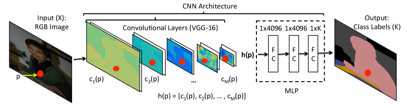
Architecture: As in past work, our architecture makes use of multiscale convolutional features, which we write as a hypercolumn descriptor:
We learn a nonlinear predictor implemented as a multi-layer perception (MLP) [7] defined over hypercolumn features. We use a MLP with ReLU activation functions, which can be implemented as a series of “fully-connected” layers. Importantly, the last layer must be of size , the number of class labels or real valued outputs being predicted. We visualize our network in Figure 1.
Dense predictions: We now describe an efficient method for generating dense pixel predictions with our network, which will be used at test-time. Dense prediction proceeds by (1) feedforward computation of convolutional responses at all layers and (2) bilinear interpolation (through “deconvolution”) of each response map to the original pixel resolution. This produces a dense grid of hypercolumn features, which are then (3) processed by pixel-wise MLPs implemented as 1x1 filters (representing each fully-connected layer). The memory intensive portion of this computation is the dense grid of hypercolumn features. This memory footprint is reasonable at test time because a single image can be processed at a time, but at train-time, we would like to train on batches containing many images as possible (to ensure diversity).
Sparse predictions: We now describe an efficient method for generating sparse pixel predictions, which will be used at train-time (for efficient mini-batch generation). Assume that we are given an image and a sparse set of (sampled) pixel locations . We efficiently generate a sparse set of predictions at those pixels as follows: we follow step (1) from above, but replace (2) with a sparse on-demand computation of hypercolumn features vectors at positions . To compute this set, we introduce a new multi-scale sampling layer (in Caffe [38]) that directly extracts the 4 convolutional features corresponding to the 4 discrete locations in closest to pixel position , and then computes via bilinear interpolation “on the fly”. This avoids the computation of a dense grid of hypercolumn features. Finally, step (3) can be implemented as a simple matrix-vector multiplication (by re-arranging the set of hypercolumn vectors into a matrix). We experimentally demonstrate that this approach offers an excellent tradeoff between amortized computation and reduced storage, given that a modest number of pixels are sampled per image. If the number of samples is very small (‘1’ in the extreme case), one can further reduce computation with sparse convolutions (implemented say, by cropping the input image around the sample). Finally, we note that our multi-scale sampling layers simply acts as a selection operation, for which a (sub) gradient can easily be defined. This means that backprop can also take advantage of sparse computations for nonlinear MLP layers and convolutional processing for the lower layers.
Mini-batch sampling: At each iteration of SGD training, the true gradient over the model parameters is approximated by computing the gradient over a relatively small set of samples from the training set. Approaches based on FCN [48] include features for all pixels from an image in a mini-batch. As nearby pixels in an image are highly correlated, sampling them may potentially hurt learning. For instance, correlated samples may overfit to earlier images and require the use of lower learning rates, which slows convergence. To ensure a diverse set of pixels (while still enjoying the amortized benefits of convolutional processing), we settled on the following strategy: rather than using all pixels from a single image, we use a modest number of pixels () per image, but sample many images per batch. Naive computation of dense grid of hypercolumn descriptors takes almost all of the (GPU) memory, while samples takes a small amount using our sparse sampling layer. This allows us to explore more images per batch, significantly increasing sample diversity (as our experiments show, Sec. 4). We explore the precise tradeoff between sampling size, number of images, and overall batch size in our experiments.
One might be tempted to think about naive “straight-forward” ways of sub-sampling with the existing architectures. One easy way to sub-sampling is to simply mask out pixel-level outputs. Naively computing a dense grid of hypercolumn descriptors and processing them with a nonlinear MLP would take more than 20X memory compared to our approach. Slightly better would be masking the hypercolumn descriptors before MLP processing, which is still 16X more expensive. We believe such “implementation details” are crucial for large-scale learning in today’s world of SGD-based CNN optimization (c.f. batch normalization [36], residual learning [32], etc).
Comparison with prior art: Unlike previous approaches (such as hypercolumns [31] and FCN [48]), our approach sub-samples hypercolumn features from convolutional layers without any up-sampling. Sub-sampling allows for the use of nonlinear functions (MLP) on such multiscale features, which in turn makes the architecture more generic (eliminating the need for task-specific normalization, scaling, or hand-tuning). As evidence, we use the same settings for three completely different problems (semantic sgmentation, surface normal estimation, and edge detection). For contrast, Xie and Tu [71] required significant modifications (such as deep supervision) to make FCNs applicable for low-level edge detection.
Long et al. [48] argued against sampling and showed how the convergence is slowed when sampling few pixels. While they experiment with % sampled pixels, we sample only % of total pixels in an image. We observed the similar behaviour when using a linear predictor (See Table 1 for more details) but this issue of convergence goes away with the use of MLP. Not only the convergence, a linear predictor may require normalization/scaling, and careful hand-tuning for different tasks (as done in [31, 48]) as features across different convolutional layers lie in different dynamic ranges. On the contrary, our nonlinear MLP can learn to automatically take care of such issues.
4 Experiments
In this section we describe our experimental evaluation. We apply our architecture (with minor modifications) to the high-level task of semantic segmentation, and the low-level task of edge detection. We show state-of-the-art111We briefly present the results of surface normal estimation here in this paper. Refer to [4] for more details. results on PASCAL-Context [53] (without requiring contextual post-processing), competitive performance on PASCAL VOC 2012 [21], and advance the state of the art on the BSDS benchmark [2]. We also perform a diagnostic evaluation of the effect of sampling and other hyperparameters/design choices.
Default network: As with other methods [13, 48, 71], we fine-tune a VGG-16 network [63]. VGG-16 has 13 convolutional layers and three fully-connected (fc) layers. The convolutional layers are denoted as {, , , , , , , , , , , , }. Following [48], we transform the last two fc layers to convolutional filters222For alignment purposes, we made a small change by adding a spatial padding of 3 cells for the convolutional counterpart of fc6 since the kernel size is ., and add them to the set of convolutional features that can be aggregated into our multi-scale hypercolumn descriptor. To avoid confusion with the fc layers in our MLP, we will henceforth denote the fc layers of VGG-16 as conv- and conv-. We use the following network architecture (unless otherwise specified): we extract hypercolumn features from conv-{, , , , } with on-demand interpolation. We define a MLP over hypercolumn features with 3 fully-connected (fc) layers of size followed by ReLU [41] activations, where the last layer outputs predictions for classes (with a soft-max/cross-entropy loss).
Default training: For all the experiments we used the publicly available Caffe library [38]. All trained models and code will be released. We make use of ImageNet-pretrained values for all convolutional layers, but train our MLP layers “from scratch” with Gaussian initialization () and dropout [64]. We fix momentum and weight decay throughout the fine-tuning process. We use the following update schedule (unless otherwise specified): we tune the network for epochs with a fixed learning rate (), reducing the rate by twice every 8 epochs until we reach .
4.1 Semantic Segmentation
Dataset. The PASCAL-Context dataset [2] augments the original sparse set of PASCAL VOC 2010 segmentation annotations [21] (defined for 20 categories) to pixel labels for the whole scene. While this requires more than categories, we followed standard protocol and evaluate on the 59-class and 33-class subsets. Though all the analysis in this paper are shown on PASCAL Context dataset [2], we also evaluated our approach on the standard PASCAL VOC-2012 dataset [21] to compare with a wide variety of approaches.
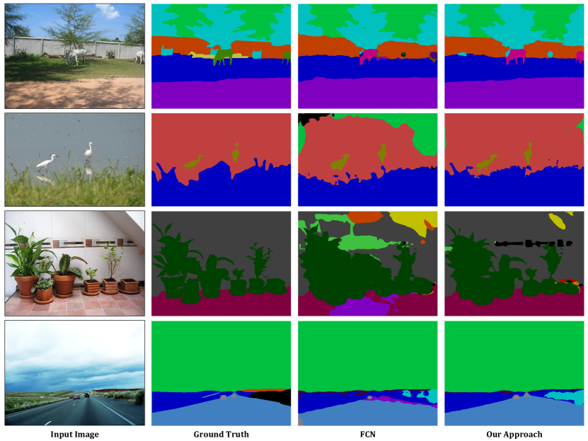
Qualitative Results. We show qualitative outputs in Figure 2 and compare against FCN-8s [48]. Notice that we capture fine-scale details, such as the leg of birds (row 2) and plant leaves (row 3).
| Settings | (%) | (%) |
|---|---|---|
| baseline (fc-3, d-4096) | 44.0 | 34.9 |
| fc-1 | 2.8 | 0.7 |
| fc-2 | 1.7 | 0.1 |
| d-1024 | 41.6 | 33.2 |
| d-2048 | 43.2 | 34.2 |
| d-6144 | 44.2 | 35.1 |
| Settings | (%) | (%) |
|---|---|---|
| baseline (2000 5) | 44.0 | 34.9 |
| 500 5 | 43.7 | 34.8 |
| 1000 5 | 43.8 | 34.7 |
| 4000 5 | 43.9 | 34.9 |
| 2000 1 | 32.6 | 24.6 |
| 10000 1 | 33.3 | 25.2 |
Evaluation Metrics. We report results on the standard metrics of pixel accuracy () and region intersection over union () averaged over classes (higher is better). Both are calculated with DeepLab evaluation tools333https://bitbucket.org/deeplab/deeplab-public/.
Analysis-1: Number of MLP fc Layers. We evaluate performance as a function of the number of MLP fc layers. Our baseline system has two -dimensional hidden layers (fc-3). We consider a linear predictor (fc-1) (implemented as a single layer) and a single -dimensional hidden layer (fc-2). Most existing architectures combining different conv layers [31, 48] are equivalent to a linear model (fc-1), while networks that operate on modified features (e.g. normalization [46], rescaling [6]) can be viewed as employing a single (designed) intermediate layer.
We found it difficult to ensure convergence for single-layer predictors with the initial learning rate of , so we reduced it to . The results of the networks using the 59-class setup can be found in Table 1 (middle rows). Everything else is kept identical during the fine-tuning process. The results are striking - models trained with fewer than 3 fc layers perform quite poorly: fc-2 constantly predicts the biggest class (“sky”) as the class label, while fc-1 behaves similarly, with some additional “background” and “person” pixels. This is consistent with [48]’s observation that random sampling of patches during training can slow convergence. We posit that such careful initialization and training schemes (like stage-wise training [48], normalization [46] or deep supervision [71]) are needed to train such networks. It is suprising that simply adding two hidden fc layers appears to significantly simplify training. Past work [46] argues that convolutional features from different layers should be normalized before concatenation. We posit that two hidden fc layers can learn such normalizations automatically, though further investigation is needed.
Analysis-2: Dimension of MLP fc Layers. Here we analyze performance as a function of the size of the MLP fc layers. We experimented the following dimensions for our fc layers: , , (baseline) and . Table 1 (left, bottom rows) lists the results. We can see that with more dimensions the network tends to learn better, potentially because it can capture more information (and with drop-out alleviating over-fitting [64]). In the following experiments we fix the size to , a good trade-off between performance and speed.
| Model | 59-class | 33-class | ||
| (%) | (%) | (%) | (%) | |
| FCN-8s [47] | 46.5 | 35.1 | 67.6 | 53.5 |
| FCN-8s [48] | 50.7 | 37.8 | - | - |
| DeepLab (v2 [12]) | - | 37.6 | - | - |
| DeepLab (v2) + CRF [12] | - | 39.6 | - | - |
| CRF-RNN [74] | - | 39.3 | - | - |
| ParseNet [46] | - | 40.4 | - | - |
| ConvPP-8 [70] | - | 41.0 | - | - |
| baseline (conv-{, , , , }) | 44.0 | 34.9 | 62.5 | 51.1 |
| conv-{, , , , , } (,) | 46.7 | 37.1 | 66.6 | 54.8 |
| conv-{, , , , , } () | 47.5 | 37.4 | 66.3 | 54.0 |
| conv-{, , , , , } (-) | 48.1 | 37.6 | 67.3 | 54.5 |
| conv-{, , , , , } (-,,) | 51.5 | 41.4 | 69.5 | 56.9 |
Analysis-3: Number of Mini-batch Samples. One of the critical questions regarding random sampling is the number of required sample. We plot performance as a function of the number of sampled pixels per image. In the first sampling experiment, we fix the batch size to images and sample , , (baseline) and pixels from each image. The results are shown in Table 2 (middle rows). We observe that: 1) even sampling only pixels per image (on average 2% of the pixels in an image) produces reasonable performance after just epochs. 2) performance is roughly constant as we increase the number of samples.
We now perform experiments where the samples are drawn from the same image. When sampling pixels from a single image (comparable in size to batch of pixels sampled from 5 images), performance dramatically drops. This phenomena consistently holds for additional pixels (Table 2, bottom rows), verifying our central thesis that statistical diversity of samples can trump the computational savings of convolutional processing during learning.
Adding conv-. While our diagnostics reveal the importance of architecture design and sampling, our best results still do not quite reach the state-of-the-art. For example, a single-scale FCN-32s [48], without any low-level layers, can already achieve . This suggests that their penultimate conv-7 layer does capture cues relevant for pixel-level prediction. In practice, we find that simply concatenating conv-7 significantly improves performance.
| Model | features (#) | fc (#) | sample (#) | Memory (MB) | Size (MB) | |
| FCN-32s [48] | 4,096 | 1 | 50,176 | 2,056 | 570 | 20.0 |
| FCN-8s [48] | 4,864 | 1 | 50,176 | 2,010 | 518 | 19.5 |
| FCN, conv-{, , }, fc-1 | 1,056 | 1 | 50,176 | 2,267 | 1,150 | 6.5 |
| FCN, conv-{, , }, fc-2 | 1,056 | 2 | 50,176 | 3,066 | 1,165 | 4.2 |
| FCN, conv-{, , }, fc-3 | 1,056 | 3 | 50,176 | 3,914 | 1,232 | 1.4 |
| FCN, conv-{, , }, fc-1 | 1,056 | 1 | 2,000 | 2,092 | 1,150 | 5.5 |
| FCN, conv-{, , }, fc-2 | 1,056 | 2 | 2,000 | 2,138 | 1,165 | 5.4 |
| FCN, conv-{, , }, fc-3 | 1,056 | 3 | 2,000 | 2,234 | 1,232 | 5.1 |
| Ours, conv-{, , }, fc-1 | 1,056 | 1 | 2,000 | 322 | 60 | 43.3 |
| Ours, conv-{, , }, fc-2 | 1,056 | 2 | 2,000 | 368 | 74 | 38.7 |
| Ours, conv-{, , }, fc-3 | 1,056 | 3 | 2,000 | 465 | 144 | 24.5 |
| Ours, conv-{, , , }, fc-3 | 5,152 | 3 | 2,000 | 1,024 | 686 | 8.8 |
Following the same training process, the results of our model with conv-7 features are shown in Table 3. From this we can see that conv-7 is greatly helping the performance of semantic segmentation. Even with reduced scale, we are able to obtain a similar achieved by FCN-8s [48], without any extra modeling of context [13, 46, 70, 74]. For fair comparison, we also experimented with single scale training with 1) half scale , and 2) full scale images. We find the results are better without training, reaching and , respectively, even closer to the FCN-8s performance ( ). For the 33-class setting, we are already doing better with the baseline model plus conv-7.
Analysis-4: Multi-scale. All previous experiments process test images at a single scale ( or its original size), whereas most prior work [13, 46, 48, 74] use multiple scales from full-resolution images. A smaller scale allows the model to access more context when making a prediction, but this can hurt performance on small objects. Following past work, we explore test-time averaging of predictions across multiple scales. We tested combinations of , and . For efficiency, we just fine-tune the model trained on small scales (right before reducing the learning rate for the first time) with an initial learning rate of and step size of epochs, and end training after epochs. The results are also reported in Table 3. Multi-scale prediction generalizes much better ( ). Note our pixel-wise predictions do not make use of contextual post-processing (even outperforming some methods that post-processes FCNs to do so [12, 74]).
Efficiency. We compared our speed, model size, and memory usage of our network to FCN [48] (same architecture) in Table 4. Removing the deconvolution layer reduces memory consumption.
PASCAL VOC-2012. Finally we use the same settings and evaluate our approach on PASCAL VOC-2012. Our approach achieves mAP of 69.7%444Per-class performance is available at http://host.robots.ox.ac.uk:8080/anonymous/PZH9WH.html.. This is much better than previous approaches, e.g. 62.7% for Hypercolumns [31], 62% for FCN [48], 67% for DeepLab (without CRF) [13] etc. Our performance on VOC-2012 is similar to Mostajabi et al [52] despite the fact we use information from only 6 layers while they used information from all the layers. In addition, they use a rectangular region of 256256 (called sub-scene) around the super-pixels. We posit that fine-tuning (or back-propagating gradients to conv-layers) enables efficient and better learning with even lesser layers, and without extra sub-scene information in an end-to-end framework. Finally, the use of super-pixels in [52] inhibit capturing detailed segmentation mask (and rather gives “blobby” output), and it is computationally less-tractable to use their approach for per-pixel optimization as information for each pixel would be required to be stored on disk.
4.2 Surface Normal Estimation
PixelNet architecture was first proposed in our work [4] on 2D-to-3D model alignment via surface normal estimation. Here we extract some of the results from [4] to show the effectiveness of this architecture for the mid-level task of surface normal estimation. The NYU Depth v2 dataset [62] is used to evaluate the surface normal maps. The criteria introduced by Fouhey et al. [25] is used to compare our approach [4] against prior work [19, 25]. Six statistics are computed over the angular error between the predicted normals and depth-based normals – Mean, Median, RMSE, 11.25∘, 22.5∘, and 30∘ – using the normals of Ladicky et al. [42] as ground truth (Note that these normals are computed from depth data obtained using kinect). The first three criteria capture the mean, median, and RMSE of angular error, where lower is better. The last three criteria capture the percentage of pixels within a given angular error, where higher is better. Table 5 compares our approach [4] with previous state-of-the-art approaches. Please refer to [4] for more details on surface normal estimation.
Unlike the task of semantic segmentation and edge detection, we use a single scale for estimating surface normal maps. We will release the results of using multi-scale approach for surface normal estimation in a future version.
4.3 Edge Detection
In this section, we demonstrate that our same architecture can produce state-of-the-art results for low-level edge detection. The standard dataset for edge detection is BSDS-500 [2], which consists of training, validation, and testing images. Each image is annotated by humans to mark out the contours. We use the same augmented data (rotation, flipping, totaling images without resizing) used to train the state-of-the-art Holistically-nested edge detector (HED) [71]. We report numbers on the testing images. During training, we follow HED and only use positive labels where a consensus ( out of ) of humans agreed.
| ODS | OIS | AP | |
|---|---|---|---|
| conv-{, , , , } Uniform | .767 | .786 | .800 |
| conv-{, , , , } (25%) | .792 | .808 | .826 |
| conv-{, , , , } (50%) | .791 | .807 | .823 |
| conv-{, , , , } (75%) | .790 | .805 | .818 |
| ODS | OIS | AP | |
| Human [2] | .800 | .800 | - |
| Canny | .600 | .640 | .580 |
| Felz-Hutt [23] | .610 | .640 | .560 |
| gPb-owt-ucm [2] | .726 | .757 | .696 |
| Sketch Tokens [44] | .727 | .746 | .780 |
| SCG [69] | .739 | .758 | .773 |
| PMI [37] | .740 | .770 | .780 |
| SE-Var [17] | .746 | .767 | .803 |
| OEF [30] | .749 | .772 | .817 |
| DeepNets [39] | .738 | .759 | .758 |
| CSCNN [34] | .756 | .775 | .798 |
| HED [71] | .782 | .804 | .833 |
| HED [71] (Updated version) | .790 | .808 | .811 |
| HED merging [71] (Updated version) | .788 | .808 | .840 |
| conv-{, , , , } (50%) | .791 | .807 | .823 |
| conv-{, , , , , } (50%) | .795 | .811 | .830 |
| conv-{, , , , } (25%)-(,) | .792 | .808 | .826 |
| conv-{, , , , , } (25%)-(,) | .795 | .811 | .825 |
| conv-{, , , , } (50%)-(,) | .791 | .807 | .823 |
| conv-{, , , , , } (50%)-(,) | .795 | .811 | .830 |
| conv-{, , , , , } (25%)-() | .792 | .808 | .837 |
| conv-{, , , , , } (50%)-() | .791 | .803 | .840 |
Baseline. We use the same baseline network that was defined for semantic segmentation, only making use of pre-trained conv layers. A sigmoid cross-entropy loss is used to determine the whether a pixel is belonging to an edge or not. Due to the highly skewed class distribution, we also normalized the gradients for positives and negatives in each batch (as in [71]).
Training. We use our previous training strategy, consisting of batches of images with a total sample size of pixels. Each image is randomly resized to half its scale (so and times) during learning. The initial learning rate is again set to . However, since the training data is already augmented, we found the network converges much faster than when training for segmentation. To avoid over-training and over-fitting, we reduce the learning rate at epochs and epochs (by a factor of ) and end training at epochs.
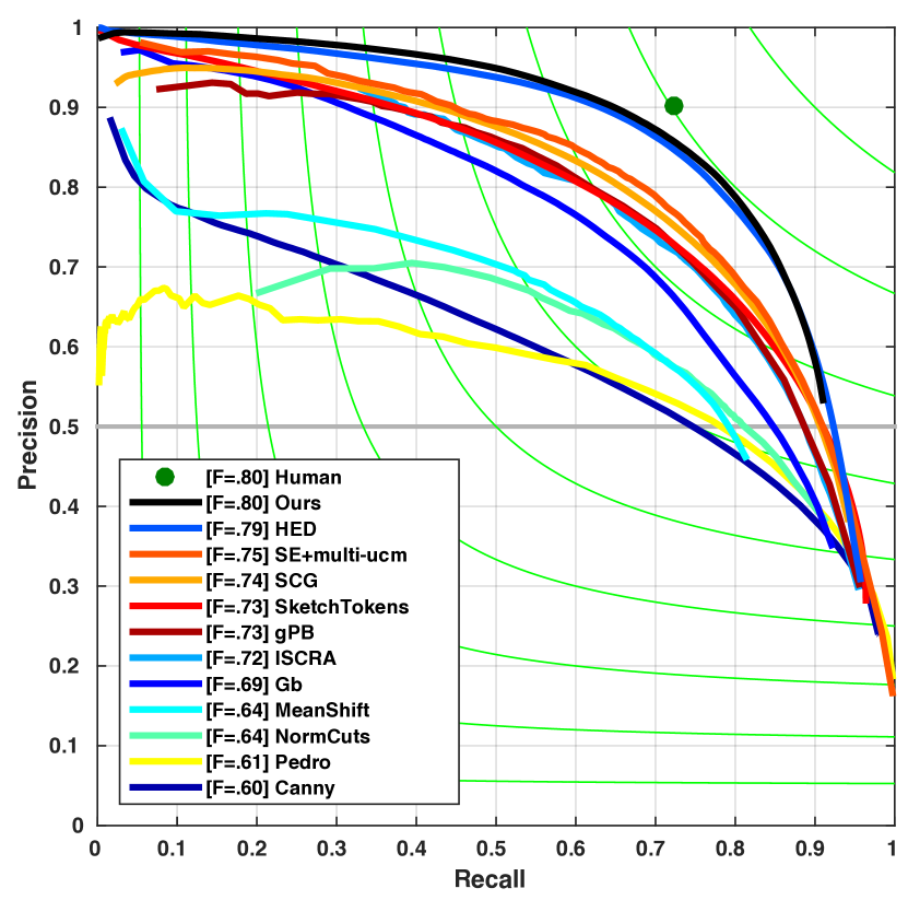
Baseline Results. The results on BSDS, along with other concurrent methods, are reported in Table 7. We apply standard non-maximal suppression and thinning technique using the code provided by [16]. We evaluate the detection performance using three standard measures: fixed contour threshold (ODS), per-image best threshold (OIS), and average precision (AP).
Analysis-1: Sampling. Whereas uniform sampling sufficed for semantic segmentation [48], we found the extreme rarity of positive pixels in edge detection required focused sampling of positives. We compare different strategies for sampling a fixed number ( pixels per image) training examples in Table 6. Two obvious approaches are uniform and balanced sampling with an equal ratio of positives and negatives (shown to be useful for object detection [26]). We tried ratios of , and , and found that balancing consistently improved performance555Note that simple class balancing [71] in each batch is already used, so the performance gain is unlikely from label re-balancing..
Analysis-2: conv-7. We previously found that adding features from higher layers is helpful for semantic segmentation. Are such high-level features also helpful for edge detection, generally regarded as a low-level task? To answer this question, we again concatenated conv-7 features with other conv layers { , , , , }. Please refer to the results at Table 7, using the second sampling strategy. We find it still helps performance a bit, but not as significantly for semantic segmentation (clearly a high-level task). Our final results as a single output classifier are very competitive to the state-of-the-art.
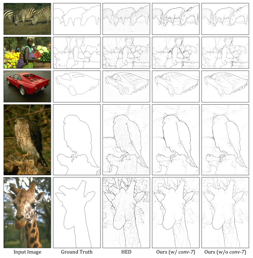
Qualitatively, we find our network tends to have better results for semantic-contours (e.g. around an object), particularly after including conv-7 features. Figure 4 shows some qualitative results comparing our network with the HED model. Interestingly, our model explicitly removed the edges inside the zebra, but when the model cannot recognize it (e.g. its head is out of the picture), it still marks the edges on the black-and-white stripes. Our model appears to be making use of much higher-level information than past work on edge detection.
5 Discussion
We have described a convolutional pixel-level architecture that, with minor modifications, produces state-of-the-art accuracy on diverse high-level, mid-level [4], and low-level tasks. We demonstrate impressive results666We ran a vanilla version of our approach for depth estimation, and achieved near state-of-the-art performance (on NYU-v2 depth dataset) with a simple scale-invariant loss function [20]. We will add the results of depth estimation after more careful analysis in a later version. on highly-benchmarked semantic segmentation, surface normal estimation [4], and edge datasets. Our results are made possible by careful analysis of computational and statistical considerations associated convolutional predictors. Convolution exploits spatial redundancy of pixel neighborhoods for efficient computation, but this redundancy also impedes learning. We propose a simple solution based on stratified sampling that injects diversity while taking advantage of amortized convolutional processing. Finally, our efficient learning scheme allow us to explore nonlinear functions of multi-scale features that encode both high-level context and low-level spatial detail, which appears relevant for most pixel prediction tasks.
Acknowledgements: This work was in part supported by NSF Grants IIS 0954083, IIS 1618903, and support from Google and Facebook. AB and XC would like to thank Abhinav Shrivastava and Saining Xie for useful discussion.
References
- [1] P. Arbeláez, B. Hariharan, C. Gu, S. Gupta, L. Bourdev, and J. Malik. Semantic segmentation using regions and parts. In CVPR. IEEE, 2012.
- [2] P. Arbelaez, M. Maire, C. Fowlkes, and J. Malik. Contour detection and hierarchical image segmentation. TPAMI, 2011.
- [3] S. Baker, D. Scharstein, J. Lewis, S. Roth, M. J. Black, and R. Szeliski. A database and evaluation methodology for optical flow. IJCV, 92(1), 2011.
- [4] A. Bansal, B. Russell, and A. Gupta. Marr Revisited: 2D-3D model alignment via surface normal prediction. In CVPR, 2016.
- [5] J. T. Barron and B. Poole. The fast bilateral solver. CoRR, abs/1511.03296, 2015.
- [6] S. Bell, C. L. Zitnick, K. Bala, and R. Girshick. Inside-outside net: Detecting objects in context with skip pooling and recurrent neural networks. arXiv preprint arXiv:1512.04143, 2015.
- [7] C. M. Bishop. Neural networks for pattern recognition. Oxford university press, 1995.
- [8] A. Bordes, L. Bottou, and P. Gallinari. Sgd-qn: Careful quasi-newton stochastic gradient descent. JMLR, 10, 2009.
- [9] L. Bottou. Large-scale machine learning with stochastic gradient descent. In Proceedings of COMPSTAT’2010, pages 177–186. Springer, 2010.
- [10] W. Byeon, T. M. Breuel, F. Raue, and M. Liwicki. Scene labeling with lstm recurrent neural networks. In CVPR, 2015.
- [11] J. Carreira, R. Caseiro, J. Batista, and C. Sminchisescu. Semantic segmentation with second-order pooling. In ECCV. 2012.
- [12] L. Chen, G. Papandreou, I. Kokkinos, K. Murphy, and A. L. Yuille. Deeplab: Semantic image segmentation with deep convolutional nets, atrous convolution, and fully connected crfs. CoRR, abs/1606.00915, 2016.
- [13] L.-C. Chen, G. Papandreou, I. Kokkinos, K. Murphy, and A. L. Yuille. Semantic image segmentation with deep convolutional nets and fully connected CRFs. In ICLR, 2015.
- [14] J. Dean, G. Corrado, R. Monga, K. Chen, M. Devin, M. Mao, A. Senior, P. Tucker, K. Yang, Q. V. Le, et al. Large scale distributed deep networks. In NIPS, 2012.
- [15] E. L. Denton, S. Chintala, R. Fergus, et al. Deep generative image models using a laplacian pyramid of adversarial networks. In NIPS, 2015.
- [16] P. Dollár and C. Zitnick. Structured forests for fast edge detection. In ICCV, 2013.
- [17] P. Dollár and C. L. Zitnick. Fast edge detection using structured forests. TPAMI, 37(8), 2015.
- [18] A. Dosovitskiy, P. Fischer, E. Ilg, P. Häusser, C. Hazrba, V. Golkov, P. v.d. Smagt, D. Cremers, and T. Brox. Flownet: Learning optical flow with convolutional networks, Dec 2015.
- [19] D. Eigen and R. Fergus. Predicting depth, surface normals and semantic labels with a common multi-scale convolutional architecture. In ICCV, 2015.
- [20] D. Eigen, C. Puhrsch, and R. Fergus. Depth map prediction from a single image using a multi-scale deep network. In NIPS, 2014.
- [21] M. Everingham, L. Van Gool, C. K. I. Williams, J. Winn, and A. Zisserman. The PASCAL Visual Object Classes (VOC) Challenge. IJCV, 2010.
- [22] C. Farabet, C. Couprie, L. Najman, and Y. LeCun. Learning hierarchical features for scene labeling. TPAMI, 35(8), 2013.
- [23] P. F. Felzenszwalb and D. P. Huttenlocher. Efficient graph-based image segmentation. IJCV, 59(2), 2004.
- [24] P. Fischer, A. Dosovitskiy, E. Ilg, P. Häusser, C. Hazırbaş, V. Golkov, P. van der Smagt, D. Cremers, and T. Brox. Flownet: Learning optical flow with convolutional networks. arXiv preprint arXiv:1504.06852, 2015.
- [25] D. F. Fouhey, A. Gupta, and M. Hebert. Data-driven 3D primitives for single image understanding. In ICCV, 2013.
- [26] R. Girshick. Fast r-cnn. In ICCV, 2015.
- [27] R. Girshick, J. Donahue, T. Darrell, and J. Malik. Rich feature hierarchies for accurate object detection and semantic segmentation. In CVPR, 2014.
- [28] G. Gkioxari, B. Hariharan, R. Girshick, and J. Malik. Using k-poselets for detecting people and localizing their keypoints. 2014.
- [29] S. Gould, R. Fulton, and D. Koller. Decomposing a scene into geometric and semantically consistent regions. In ICCV. IEEE, 2009.
- [30] S. Hallman and C. C. Fowlkes. Oriented edge forests for boundary detection. In CVPR, 2015.
- [31] B. Hariharan, P. Arbeláez, R. Girshick, and J. Malik. Hypercolumns for object segmentation and fine-grained localization. In CVPR, 2015.
- [32] K. He, X. Zhang, S. Ren, and J. Sun. Deep residual learning for image recognition. arXiv preprint arXiv:1512.03385, 2015.
- [33] L. Huang, Y. Yang, Y. Deng, and Y. Yu. Densebox: Unifying landmark localization with end to end object detection. arXiv preprint arXiv:1509.04874, 2015.
- [34] J.-J. Hwang and T.-L. Liu. Pixel-wise deep learning for contour detection. arXiv preprint arXiv:1504.01989, 2015.
- [35] A. Hyvärinen, J. Hurri, and P. O. Hoyer. Natural Image Statistics: A Probabilistic Approach to Early Computational Vision., volume 39. Springer Science & Business Media, 2009.
- [36] S. Ioffe and C. Szegedy. Batch normalization: Accelerating deep network training by reducing internal covariate shift. In D. Blei and F. Bach, editors, Proceedings of the 32nd International Conference on Machine Learning (ICML-15), pages 448–456. JMLR Workshop and Conference Proceedings, 2015.
- [37] P. Isola, D. Zoran, D. Krishnan, and E. H. Adelson. Crisp boundary detection using pointwise mutual information. In Computer Vision–ECCV 2014, pages 799–814. Springer, 2014.
- [38] Y. Jia, E. Shelhamer, J. Donahue, S. Karayev, J. Long, R. Girshick, S. Guadarrama, and T. Darrell. Caffe: Convolutional architecture for fast feature embedding. In ACMMM, 2014.
- [39] J. J. Kivinen, C. K. Williams, N. Heess, and D. Technologies. Visual boundary prediction: A deep neural prediction network and quality dissection. In AISTATS, volume 1, page 9, 2014.
- [40] P. Krähenbühl and V. Koltun. Efficient inference in fully connected crfs with gaussian edge potentials. In NIPS, 2011.
- [41] A. Krizhevsky, I. Sutskever, and G. E. Hinton. Imagenet classification with deep convolutional neural networks. In NIPS, 2012.
- [42] L. Ladicky, B. Zeisl, and M. Pollefeys. Discriminatively trained dense surface normal estimation. In ECCV, 2014.
- [43] Y. A. LeCun, L. Bottou, G. B. Orr, and K.-R. Müller. Efficient backprop. In Neural networks: Tricks of the trade, pages 9–48. Springer, 2012.
- [44] J. Lim, C. Zitnick, and P. Dollár. Sketch tokens: A learned mid-level representation for contour and object detection. In CVPR, 2013.
- [45] C. Liu, J. Yuen, and A. Torralba. Nonparametric scene parsing via label transfer. TPAMI, 33(12), 2011.
- [46] W. Liu, A. Rabinovich, and A. C. Berg. Parsenet: Looking wider to see better. arXiv preprint arXiv:1506.04579, 2015.
- [47] J. Long, E. Shelhamer, and T. Darrell. Fully convolutional networks for semantic segmentation. CoRR, abs/1411.4038, 2014.
- [48] J. Long, E. Shelhamer, and T. Darrell. Fully convolutional models for semantic segmentation. In CVPR, 2015.
- [49] J. M. M. Holschneider, R. Kronland-Martinet and P. Tchamitchian. A real-time algorithm for signal analysis with the help of the wavelet transform. In Wavelets, Time-Frequency Methods and Phase Space, pages 289–297, 1989.
- [50] D. R. Martin, C. C. Fowlkes, and J. Malik. Learning to detect natural image boundaries using local brightness, color, and texture cues. TPAMI, 26(5), 2004.
- [51] O. Matan, C. J. Burges, Y. LeCun, and J. S. Denker. Multi-digit recognition using a space displacement neural network. In NIPS, pages 488–495, 1991.
- [52] M. Mostajabi, P. Yadollahpour, and G. Shakhnarovich. Feedforward semantic segmentation with zoom-out features. In CVPR, pages 3376–3385, 2015.
- [53] R. Mottaghi, X. Chen, X. Liu, N.-G. Cho, S.-W. Lee, S. Fidler, R. Urtasun, and A. Yuille. The role of context for object detection and semantic segmentation in the wild. In CVPR, 2014.
- [54] D. Munoz, J. A. Bagnell, and M. Hebert. Stacked hierarchical labeling. In Computer Vision–ECCV 2010, pages 57–70. Springer, 2010.
- [55] H. Noh, S. Hong, and B. Han. Learning deconvolution network for semantic segmentation. In ICCV, 2015.
- [56] P. H. Pinheiro and R. Collobert. Recurrent convolutional neural networks for scene parsing. In ICML, 2014.
- [57] J. C. Platt and R. Wolf. Postal address block location using a convolutional locator network. In NIPS, 1993.
- [58] D. Ramanan. Learning to parse images of articulated bodies. In NIPS. 2007.
- [59] C. Russell, P. Kohli, P. H. Torr, et al. Associative hierarchical crfs for object class image segmentation. In ICCV. IEEE, 2009.
- [60] A. Saxena, S. H. Chung, and A. Y. Ng. 3-d depth reconstruction from a single still image. IJCV, 76(1), 2008.
- [61] J. Shotton, J. Winn, C. Rother, and A. Criminisi. Textonboost for image understanding: Multi-class object recognition and segmentation by jointly modeling texture, layout, and context. Int. Journal of Computer Vision (IJCV), January 2009.
- [62] N. Silberman, D. Hoiem, P. Kohli, and R. Fergus. Indoor segmentation and support inference from rgbd images. In ECCV, 2012.
- [63] K. Simonyan and A. Zisserman. Very deep convolutional networks for large-scale image recognition. CoRR, abs/1409.1556, 2014.
- [64] N. Srivastava, G. Hinton, A. Krizhevsky, I. Sutskever, and R. Salakhutdinov. Dropout: A simple way to prevent neural networks from overfitting. JMLR, 15(1), 2014.
- [65] J. Tighe and S. Lazebnik. Superparsing: scalable nonparametric image parsing with superpixels. In Computer Vision–ECCV 2010, pages 352–365. Springer, 2010.
- [66] Z. Tu and X. Bai. Auto-context and its application to high-level vision tasks and 3d brain image segmentation. TPAMI, 32(10), 2010.
- [67] L. Wang, W. Ouyang, X. Wang, and H. Lu. Visual tracking with fully convolutional networks. In ICCV, 2015.
- [68] X. Wang, D. Fouhey, and A. Gupta. Designing deep networks for surface normal estimation. In CVPR, 2015.
- [69] R. Xiaofeng and L. Bo. Discriminatively trained sparse code gradients for contour detection. In NIPS, 2012.
- [70] S. Xie, X. Huang, and Z. Tu. Convolutional pseudo-prior for structured labeling. arXiv preprint arXiv:1511.07409, 2015.
- [71] S. Xie and Z. Tu. Holistically-nested edge detection. In ICCV, 2015.
- [72] J. Yao, S. Fidler, and R. Urtasun. Describing the scene as a whole: Joint object detection, scene classification and semantic segmentation. In CVPR. IEEE, 2012.
- [73] F. Yu and V. Koltun. Multi-scale context aggregation by dilated convolutions. In ICLR, 2016.
- [74] S. Zheng, S. Jayasumana, B. Romera-Paredes, V. Vineet, Z. Su, D. Du, C. Huang, and P. H. Torr. Conditional random fields as recurrent neural networks. In ICCV, 2015.