To my mother,
my father and my sister.

Abstract

This work is divided into two parts. First, we analyze the existence of positive bound and ground states for a second order stationary system coming from a coupled system of nonlinear Schrödinger–Korteweg-de Vries equations. Second, we extend these results for a higher order system of nonlinear Schrödinger–Korteweg-de Vries equations. Looking for “standing-traveling” waves we arrive at a bi-harmonic stationary system, for which we prove the existence and multiplicity of solutions under appropriate conditions on the parameters.

Resumen

Este trabajo está dividido en dos partes. Primero, se analiza la existencia de soluciones de un sistema estacionario de segundo orden que proviene de un sistema no linear tipo Schrödinger–Korteweg-de Vries. La otra parte del trabajo está dedicada al estudio un sistema no lineal de alto orden también de tipo Schrödinger–Korteweg-de Vries. Buscando soluciones en forma de onda “estacionaria-viajera” se obtiene un sistema biarmónico estacionario, para el cual se demuestra la existencia y multiplicidad de soluciones bajo determinadas condiciones de los parámetros.

Notations

$L^{p}(\Omega)$	Lebesgue space with norm $\|\cdot\|_{L^{p}}$.
$L^{q}_{loc}(\Omega)$	Space of functions $f:\Omega\to\mathbb{R}$ such that $f\in L^{p}(K)$ for every compact set $K\subset\Omega$.
$\mathcal{C}(\Omega)$	Space of continuous functions in $\Omega$.
$\mathcal{C}^{n}(\Omega)$	Space of $n$ times continuously differentiable functions in $\Omega$.
$\mathcal{C}^{\infty}(\Omega)$	Space of infinitely differentiable functions in $\Omega$.
$\mathcal{C}_{c}(\Omega)$	Space of functions with compact support in $\Omega$.
$\mathcal{C}_{c}^{\infty}(\Omega)$	Space of infinitely differentiable functions with compact support in $\Omega$.
$\mathbb{R}^{N}_{+}=\{(x^{\prime},x_{N})\in\mathbb{R}^{N}\ :x_{N}>0\ \}$	Set with the last component $x_{N}>0$.
${\bf Q}=\{(x^{\prime},x_{N})\in\mathbb{R}^{N}:|x^{\prime}|<1,\ |x_{N}|<1\}$	Set with the last component $x_{N}<1$ and $x^{\prime}$ in the unit ball in $\mathbb{R}^{N-1}$.
${\bf Q}_{+}={\bf Q}\cap\mathbb{R}^{N}_{+}$	Intersection between ${\bf Q}$ and $\mathbb{R}^{N}_{+}$.
${\bf Q}_{0}=\{(x^{\prime},0)\in\mathbb{R}^{N}\ :|x^{\prime}|<1\}$	Set with $x^{\prime}$ in the unit ball in $\mathbb{R}^{N-1}$ and $x_{N}=0$.
$W^{m,p}(\Omega)$	Sobolev space with $m$ derivatives in $L^{p}(\Omega)$.
$W^{m,p}_{r}(\Omega)$	Space of the radially symmetric functions belong $W^{m,p}(\Omega)$.
$W^{m,p}_{rd}(\Omega)$	Space of the non-increasing radially symmetric functions belong $W^{m,p}(\Omega)$.
$L(X,Y)$	Set of the linear continuous maps from $X$ into $Y$.
$L_{k}(X,Y)$	Space of $k$-linear maps from $X$ into $Y$.
$\mathcal{C}(\mathcal{U},Z)$	Set of continuous maps from $\mathcal{U}$ onto $Z$.

$\mathcal{C}^{k}(\mathcal{U},Z)$	Subset of $\mathcal{C}(\mathcal{U},Z)$ of $k$ times differentiable maps $J$ such that the application $\mathcal{U}\to L_{k}(X,\mathbb{R})$, defined as $u\mapsto d^{k}J(u)$, is continuous.
$\mathcal{C}^{0,\alpha}(\mathcal{U},Z)$	Set of maps $J\in\mathcal{C}(\mathcal{U},Z)$ such that $$\sup\limits_{\begin{subarray}{c}u,v\in\mathcal{U}\\ u\neq v\end{subarray}}\left(\frac{|J(u)-J(v)|}{\|u-v\|^{\alpha}}\right)<+\infty$$ for some $\alpha\in(0,1]$. If $\alpha=1$ these maps are called Lipschitz continuous and if $\alpha<1$ these maps are nothing but the Hölder continuous maps.
$\mathcal{C}^{k,\alpha}(\mathcal{U},Z)$	Set of maps $J\in\mathcal{C}^{k}(\mathcal{U},Z)$ such that $d^{k}J(u)\in\mathcal{C}^{0,\alpha}(\mathcal{U},Z)$.
$\Omega^{\star}$	Symmetrized set of $\Omega$
$u^{\star}$	Schwarz symmetrization of function $u$
$\hbar$	Reduced Planck constant (Planck constant divided by $2\pi$)
$\displaystyle\nabla=\left(\frac{\partial}{\partial x_{1}},\frac{\partial}{\partial x_{2}},\dots,\frac{\partial}{\partial x_{N}}\right)$	Gradient differential operator
$\displaystyle\Delta=\left(\frac{\partial^{2}}{\partial x_{1}^{2}}+\frac{\partial^{2}}{\partial x_{2}^{2}}+\dots+\frac{\partial^{2}}{\partial x_{N}^{2}}\right)$	Laplacian differential operator
$\langle\cdot,\cdot\rangle_{H}$	Scalar product in the Hilbert space $H$.
$\|\cdot\|_{X}$	Norm in the space X.
$X^{\prime}$	Dual space of $X$
$\hookrightarrow$	Continuous embedding.
$\hookrightarrow\hookrightarrow$	Compact embedding.
$\rightharpoonup$	Weak Convergence.
$a.e.$	Convergence almost everywhere.
$f|_{\Omega}$	Restriction of function $f$ to $\Omega$.
$\mathcal{F}|_{\Omega}$	Set of functions $f\in\mathcal{F}$ restricted to $\Omega$.
$\omega_{N}$	Volume of the unit ball in $\mathbb{R}^{N}$.
$\omega_{N}^{\prime}$	Surface of the unit sphere in $\mathbb{R}^{N}$.
$T_{p}M$	Tangent space to $M$ at the point $p\in M$.
$\oplus$	Direct sum.
$d_{G}J$	Gâteaux differential of $J$.
$dJ$	Fréchet differential of $J$.
$d_{M}J$	Constrained derivative of $J$ on a manifold $M.$
$\nabla_{M}$	Constrained gradient of $J$ on $M$.
$\mathcal{H}_{N}X$	$N$-dimensional (Hausdorff) measure of the set $X$.

Introduction

This work aims to prove the existence of solutions for two coupled systems of partial differential equations.

The first system is composed by a nonlinear Schrödinger equation and a Korteweg-de Vries equation as follows

$$\boxed{\left\{\begin{array}[]{rcl}if_{t}+f_{xx}+|f|^{2}f+\beta fg&=&0\\ g_{t}+g_{xxx}+gg_{x}+\frac{1}{2}\beta(|f|^{2})_{x}&=&0,\end{array}\right.}$$ (S1)

where $f=f(x,t)\in\mathbb{C}$ while $g=g(x,t)\in\mathbb{R}$, and $\beta\in\mathbb{R}$ is the real coupling coefficient. System (S1) appears in phenomena of interactions between short and long dispersive waves, arising in fluid mechanics, such as the interactions of capillary-gravity water waves. Indeed, $f$ represents the short wave, while $g$ stands for the long wave. See [3, 28, 29, 30, 43] and the references therein for more details. We look for solitary “traveling” waves solutions, namely solutions to (S1) of the form

$$(f(x,t),g(x,t))=\left(e^{i\omega t}e^{i\frac{c}{2}x}u(x-ct),v(x-ct)\right),$$

with $u$ and $v$ real functions. Choosing $\lambda_{1}=\omega+\frac{c^{2}}{4}$, $\lambda_{2}=c$, we get that $u,\,v$ solve the following stationary problem in dimension one

$$\left\{\begin{array}[]{rcl}-u^{\prime\prime}+\lambda_{1}u&=&u^{3}+\beta uv\\ -v^{\prime\prime}+\lambda_{2}v&=&\frac{1}{2}v^{2}+\frac{1}{2}\beta u^{2}.\end{array}\right.$$ (1)

This system has been previously studied by Dias, Figueira and Oliveira in [33]. Also, a generalization of (1) with general power nonlinearities, has been previously analyzed by the same authors in [34] and by Albert and Bhattarai in [4]. The results obtained in the works previously mentioned were improved in several points in [28]. In this work, we focus our attention on one of these points which deals with the existence of positive even ground and bound states of (1) under the appropriate range of parameter settings. We mainly perform a detailed analysis of the recent work [28, 29], where positive solutions of (1) are classified proving:

• Existence of positive even ground states of (1) under the following hypotheses:

  • the coupling coefficient $\beta>\Lambda>0$ for an appropriate constant $\Lambda$; see Theorem 2.3.1,

  • $\beta>0$ and $\lambda_{2}\gg 1$; see Theorem 2.3.2.

• Existence of positive even bound states of (1) when:

  • $0<\beta\ll 1$; see Theorem 2.3.3, where we also give a bifurcation result,

  • $0<\beta<\Lambda$ and $\lambda_{2}\gg 1$; see Theorem 2.3.4.

We also extend these results to dimensions $N=2,3$. The coexistence of positive bound and ground states for $0<\beta<\Lambda$ and $\lambda_{2}$ large is a great novelty due to the difference with the more studied systems of nonlinear Schrödinger equations in the last several years; see Remark 2.3.5.

The second system that we study is a higher order system coming from (1) as a natural extension. More precisely, we consider the following system

$$\boxed{\left\{\begin{array}[]{rcl}if_{t}-f_{xxxx}+|f|^{2}f+\beta fg&=&0\\ g_{t}-g_{xxxxx}+|g|g_{x}+\tfrac{1}{2}\beta(|f|^{2})_{x}&=&0.\end{array}\right.}$$ (S2)

Looking for “standing-traveling” waves solutions of the form

$$(f(x,t),g(x,t))=\left(e^{i\lambda_{1}t}u(x),v(x-\lambda_{2}t)\right),$$

with $u$ and $v$ real functions, we arrive at the fourth-order stationary system

$$\left\{\begin{array}[]{ccl}u^{(iv}+\lambda_{1}u&=&u^{3}+\beta uv\\ v^{(iv}+\lambda_{2}v&=&\frac{1}{2}|v|v+\frac{1}{2}\beta u^{2},\end{array}\right.$$ (2)

where $w^{(iv}$ denotes the fourth derivative of $w$. This is the first time, up to our knowledge, that the interaction of standing waves and traveling waves is analyzed in the mathematical literature. Although system (S2) only make sense in dimension $N=1$, we can consider the stationary system (2) in higher dimensional cases

$$\left\{\begin{array}[]{ccl}\Delta^{2}u+\lambda_{1}u&=&u^{3}+\beta uv\\ \Delta^{2}v+\lambda_{2}v&=&\frac{1}{2}|v|v+\frac{1}{2}\beta u^{2},\end{array}\right.$$ (3)

where $u,v\in W^{2,2}(\mathbb{R}^{N})$, $1\leq N\leq 7$, $\lambda_{j}>0$ with $j=1,2$ and $\beta>0$ is the coupling parameter.

Recently, other similar fourth-order systems studying the interaction of coupled nonlinear Schrödinger equations have appeared, for example in [6], where the coupling terms have the same homogeneity as the nonlinear terms. Note that, as far as we know, there is no previous mathematical work analyzing a higher order system with the nonlinear and coupling terms considered in (3).

In system (3), we first analyze the dimensional cases $2\leq N\leq 7$ in the radial framework by using the compactness described in Remark 3.2.3-$(iii)$. The one dimensional case is also studied through the application of a measure lemma due to P. L. Lions [60] to circumvent the lack of compactness. To be more precise, we prove that there exists a positive critical value of the coupling parameter $\beta$, denoted by $\Lambda^{\prime}$ and defined by (3.26), such that the associated functional constrained to the corresponding Nehari manifold possesses a positive global minimum. We show that this positive global minimum is a critical point with energy below the energy of the semi-trivial solution under the following hypotheses: either $\beta>\Lambda^{\prime}$, or $\beta>0$ and $\lambda_{2}\gg 1$. Furthermore, we find a mountain pass critical point if $\beta<\Lambda^{\prime}$ and $\lambda_{2}\gg 1$.

This work is organized as follows. In Chapter 1 we present some preliminaries necessary for the proper understanding of the results and the sake of completeness. The Schrödinger equations and the Korteweg-de Vries equation are introduced with a brief historical summaries of their discoveries. We recall the Sobolev spaces and their most important properties. Basic concepts of calculus of variation are included, such as the Palais-Smale compactness condition and the Mountain Pass Theorem. We also present some results about the Schwarz symmetrization that will be useful for our work, especially in the second chapter.

Chapter 2 is devoted to the study of system (S1). In Section 2.1 we introduce the functional framework and give some definitions. Next, we define the Nehari Manifold in Section 2.2, proving some properties of it. We establish a useful measure lemma and show a result dealing with qualitative properties of the semi-trivial solution. Section 2.3 is divided into two subsections; the first one contains the proof of the existence of ground states, and the second one deals with the existence of bound states.

In Chapter 3, we perform the corresponding analysis of the fourth order system (S2). In Section 3.1, we introduce the notation, establish the functional framework, define the Nehari manifold and study its properties. Section 3.3 is devoted to prove the main results. It is divided into two subsections; in the first one we study the high-dimensional case ($2\leq N\leq 7$), while the second one deals with the one-dimensional case.

CHAPTER 1   Preliminaries

In this chapter we present the Schrödinger equation and the Korteweg-de Vries equation. We also discuss some preliminary notions that we are going to use throughout this work.

§ 1.1.  The Schrödinger equation

In quantum mechanics, the Schrödinger equation is a partial differential equation that describes how the quantum state of a quantum system changes with time. It was formulated in 1926 by the Austrian physicist Erwin Schrödinger [75]. In classical mechanics, Newton’s second law ($F=ma$) is used to mathematically predict the state of a given system at any time after a known initial condition. In quantum mechanics, the analogue of Newton’s law is Schrödinger equation for a quantum system (usually atoms, molecules, and subatomic particles). The Schrödinger equation is a linear partial differential equation, describing the time-evolution of the system’s “wave function” (also called a “state function”) [46]. Although Schrödinger equation is often presented as a separate postulate, some authors [17, §3] show that some properties resulting from the Schrödinger equation may be deduced just from symmetry principles alone; for example, the commutation relations. Generally, “derivations” of the Schrödinger equation demonstrate its mathematical plausibility for describing wave-particle duality but, to date, there are no universally accepted derivations of the Schrödinger equation from appropriate axioms. In the Copenhagen interpretation of quantum mechanics, the wave function is the most complete description that can be given of a physical system. The Schrödinger equation describes not only molecular, atomic, and subatomic systems, but also macroscopic systems, possibly even the whole universe. This equation, in its most general form, is consistent with both classical mechanics and special relativity, but the original formulation by Schrödinger himself was non-relativistic.

The Schrödinger equation takes the form

$$i\hbar\,f_{t}=\widehat{H}f,$$ (1.1)

where $i$ is the imaginary unit, $\hbar$ is the reduced Planck constant, $f=f(\mathbf{x},t)$ is a complex wave function on $\mathbb{R}^{N}\times\mathbb{R}$, $f_{t}$ denote $\partial f/\partial t$ and $\widehat{H}$ is a Hamiltonian operator which characterizes the total energy of a given wave function and takes different forms depending on the physical situation. The best known example of this kind of equation is the non-relativistic Schrödinger equation for a single particle moving in an external field

$$i\hbar\,f_{t}=\left[-\frac{\hbar}{2\mu}\Delta+V\right]f,$$ (1.2)

where $\widehat{H}$ was taken as the total energy equals kinetic energy plus potential energy, $\Delta$ is the Laplacian differential operator and $\mu$ is the reduced mass. Rescaling (1.2) by

$$f^{\prime}(\mathbf{x}^{\prime},t)=f(\mathbf{x},t),\qquad\mathbf{x}^{\prime}=\sqrt{2\mu}\mathbf{x},$$ (1.3)

and taking a nonlinear variation of the form

$$V=-\hbar J(|f^{\prime}|^{2}),$$

for a given smooth complex function $J$, we obtain (omitting primes) the so called nonlinear Schrödinger equation

$$if_{t}+\Delta f+J(|f|^{2})f=0.$$ (1.4)

The nonlinear Schrödinger equation is a classical field equation whose principal applications are related to the propagation of light in nonlinear optical fibers and planar waveguides [76], and Bose-Einstein condensates confined to highly anisotropic cigar-shaped traps, in the mean-field regime [69]. Additionally, the equation appears in the studies of small-amplitude gravity waves on the surface of deep inviscid (zero-viscosity) water [76], the Langmuir waves in the plasma [76], the propagation of plane-diffracted wave beams in the focusing regions of the ionosphere [48], the propagation of Davydov’s alpha-helix solitons, which are responsible for energy transport along molecular chains [16], and many others. More generally, the nonlinear Schrödinger equation appears as one of the universal equations that describe the evolution of slowly varying packets of quasi-monochromatic waves in weakly nonlinear media that have dispersion [76].

In particular, the one-dimensional nonlinear Schrödinger equation is an example of an integrable model. In quantum mechanics, the one-dimensional nonlinear Schrödinger equation is a special case of the classical nonlinear Schrödinger field, which in turn is a classical limit of a quantum Schrödinger field. Both the quantum and the classical one-dimensional nonlinear Schrödinger equation are integrable. In more than one dimension, the equation is not integrable. It allows us a collapse and wave turbulence [40].

Another important equation related to the Schrödinger equation is the so called fractional Schrödinger equation, which is a fundamental equation of fractional quantum mechanics. It was introduced by Nick Laskin in 1999 (see [55, 56]) as a result of extending the Feynman path integral, from the Brownian-like to Lévy-like quantum mechanical paths. The term fractional Schrödinger equation was coined by Nick Laskin who made a generalization of standard quantum mechanics called fractional quantum mechanics. The fractional Schrödinger equation is obtained form (1.1) replacing $\widehat{H}$ by a fractional Hamiltonian operator $\widehat{H}_{\alpha}$ of the from

$$\widehat{H}_{\alpha}=D_{\alpha}(-\hbar^{2}\Delta)^{\alpha/2}+V,$$ (1.5)

where $D_{\alpha}$ is a scale constant, $(-\hbar^{2}\Delta)^{\alpha/2}$ is the quantum Riesz fractional derivative. The most common case in the literature of this equation is the three-dimensional case, in which the 3D quantum Riesz fractional derivative is given by

$$(-\hbar^{2}\Delta)^{\alpha/2}f(\mathbf{x},t)=\frac{1}{(2\pi\hbar)^{3}}\int_{\mathbb{R}^{3}}e^{i\frac{\mathbf{p}\mathbf{x}}{\hbar}}|\mathbf{p}|^{\alpha}\widehat{f}(\mathbf{p},t)\,d\mathbf{p},$$

where

$$\widehat{f}(\mathbf{p},t)=\int_{\mathbb{R}^{3}}e^{-i\frac{\mathbf{p}\mathbf{x}}{\hbar}}f(\mathbf{x},t)\,d\mathbf{x},$$

is the three-dimensional Fourier transform of $f$. The index $1<\alpha\leq≤2$ in the above expression is the so called Lèvy index. Thus, the fractional Schrödinger equation includes a space derivative of fractional order $\alpha$ instead of the second order space derivative in the standard Schrödinger equation. At $\alpha=2$, the fractional Schrödinger equation becomes the standard Schrödinger equation. There are many applications of the fractional Schrödinger equation such as the fractional Bohr atom, the fractional quantum oscillator, the fractional quantum mechanics in solid state systems, and others; see [47] for more applications.

§ 1.2.  The Korteweg-de Vries equation

The Korteweg-de Vries equation is a universal mathematical model for the description of weakly nonlinear long wave propagation in dispersive media. This equation is given by

$$g_{t}+\alpha gg_{x}+\beta g_{xxx}=0,$$ (1.6)

where $g(x,t)$ is a real function of the one-dimensional space coordinate $x$ and time $t$. The coefficients $\alpha$ and $\beta$ are determined by the medium properties and can be either constants or functions.

An incomplete list of physical applications of the Korteweg-de Vries equations includes shallow-water gravity waves [49], ion-acoustic waves in collisionless plasma [65, 38], waves in bubbly fluids [52], waves in the ocean and many others [31]. This broad range of applicability is explained by the fact that the Korteweg-de Vries equation describes a combined effect of the lowest-order, quadratic, nonlinearity (term $gg_{x}$) and the simplest long-wave dispersion (term $g_{xxx}$). One can find derivations of the Korteweg-de Vries equation for different physical contexts in the books by Dodd et al [35], Drazin and Johnson [36], Newell [68], and others.

Although the Korteweg-de Vries equations with constant coefficient was originally derived in the second half of the 19th century, its real significance as a fundamental mathematical model for the generation and propagation of long nonlinear waves of small amplitude has been understood only after the seminal works of Zabusky and Kruskal (1965)[80], Gardner, Greene, Kruskal and Miura (1967)[45] and Lax (1968)[57]. These authors showed that the Korteweg-de Vries equation (unlike a “general” nonlinear dispersive equation) can be solved exactly for a broad class of initial or boundary conditions and, importantly, the solutions often contain a combination of localized wave states, which preserve their “identity” in the interactions with each other; pretty much as classical particles do. In the longtime asymptotic solutions, such localized states represent solitary waves, which are waves that maintain their shape while propagating at a constant speed. Such solitary wave solutions of the Korteweg-de Vries equation have been called solitons by Zabusky and Kruskal in 1965 [80] owing to their unusual particle-like behaviour in the interactions with other solitary waves and nonlinear radiation. However, the solitons were already well known due to the original works of Russel (1845) [73], Boussinesq (1972) [21], Rayleigh (1876), and Korteweg and de Vries (1895) [53].

When $\alpha$ y $\beta$ are constant, the Korteweg-de Vries equation can be rescaled in order to eliminate the constants. Setting

$$g^{\prime}(x^{\prime},t^{\prime})=\alpha g(x,t),\qquad x^{\prime}=\frac{x}{\sqrt{\beta}},\qquad t^{\prime}=\frac{t}{\sqrt{\beta}},$$ (1.7)

equation (1.6) takes the form (omitting primes),

$$g_{t}+gg_{x}+g_{xxx}=0.$$ (1.8)

We shall look for a solution of the above equation in the form of a traveling wave, i.e., $g(x,t)=v(\theta)$, where $\theta=x-ct$ is the travelling phase and $c$ is the phase velocity. Moreover, we assume that $v,v^{\prime}$ and $v^{\prime\prime}$ vanish at infinity where, now, $v^{\prime}$ and $v^{\prime\prime}$ represent the first and second derivative respectively of $v$. Now, the Korteweg-de Vries equation reduces to an ordinary differential equation for the function $v$ as follows

Figure 1.1: Soliton

$$-cv^{\prime}+vv^{\prime}+v^{\prime\prime\prime}=0,$$ (1.9)

which integrated gives us

$$-cv+\frac{v^{2}}{2}+v^{\prime\prime}+c_{1}=0.$$ (1.10)

Taking into account that $v$ vanishes at infinity it follows that $c_{1}=0$, and performing the change of variable $v(\theta)=2cV(\sqrt{c}\theta)$ we get

$$V^{\prime\prime}-V+V^{2}=0.$$ (1.11)

We can see in [54] that the above equation has a unique positive even solution given by

$$V(\theta)=\frac{3}{2\cosh^{2}\left(\frac{\theta}{2}\right)}.$$ (1.12)

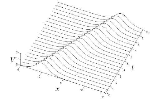
Taking into account that $\theta=x-ct$, the expression (1.12) describes a right-moving soliton (see Figure 1.1).

§ 1.3.  Sobolev spaces

In this section we will present the Sobolev spaces and some of their properties.

Let $\Omega\subset\mathbb{R}^{N}$ be an open set.

Definition 1.3.1.

For $1\leq p\leq\infty$, the Sobolev space $W^{1,p}(\Omega)$ is defined by

$$W^{1,p}(\Omega)=\left\{u\in L^{p}(\Omega)\left|\begin{array}[]{l}\exists\ g_{1},g_{2},\dots,g_{N}\in L^{p}(\Omega)\qquad\text{such that}\\ \displaystyle\int_{\Omega}u\frac{\partial\varphi}{\partial x_{i}}=-\displaystyle\int_{\Omega}g_{i}\varphi\quad\forall\varphi\in\mathcal{C}_{c}^{\infty}(\Omega),\quad\forall i=1,2,\dots,N\end{array}\right.\right\}.$$

For $u\in W^{1,p}(\Omega)$ we define the weak partial derivatives and gradient as follows

$$\frac{\partial u}{\partial x_{i}}=g_{i},\qquad\nabla u=\left(\frac{\partial u}{\partial x_{1}},\frac{\partial u}{\partial x_{2}},\dots,\frac{\partial u}{\partial x_{N}}\right).$$

The space $W^{1,p}(\Omega)$ is equipped with the norm

$$\|u\|_{W^{1,p}}=\|u\|_{L^{p}}+\sum\limits_{i=1}^{N}\left\|\frac{\partial u}{\partial x_{i}}\right\|_{L^{p}},$$ (1.13)

which, for $1\leq p<\infty$, is equivalent to the norm

$$\|u\|_{W^{1,p}}=\left(\|u\|_{L^{p}}^{p}+\|\nabla u\|_{L^{p}}^{p}\right)^{\frac{1}{p}},$$ (1.14)

where

$$\|\nabla u\|_{L^{p}}=\left(\sum\limits_{i=1}^{N}\left\|\frac{\partial u}{\partial x_{i}}\right\|_{L^{p}}^{p}\right)^{\frac{1}{p}}.$$

Now we will introduce the Sobolev spaces with higher orders of regularity.

Definition 1.3.2.

Let $m\geq 2$ be an integer and $1\leq p\leq\infty$, then, we define by induction the set $W^{m,p}(\Omega)$

$$W^{m,p}(\Omega)=\left\{u\in W^{m-1,p}(\Omega)\left|\ \frac{\partial u}{\partial x_{i}}\in W^{m-1,p}(\Omega),\quad\forall i=1,2,\dots,N\right.\right\}.$$

We use the standard multi-index notation $\alpha=(\alpha_{1},\alpha_{2},\dots,\alpha_{N})$, with $\alpha_{i}\geq 0$ integers, to denote the weak partial derivatives as follows,

$$D^{\alpha}u=\frac{\partial^{|\alpha|}u}{\partial x_{1}^{\alpha_{1}}\partial x_{2}^{\alpha_{2}},\cdots,\partial x_{N}^{\alpha_{N}}},\quad\text{where}\quad|\alpha|=\sum\limits_{i=1}^{N}\alpha_{i}\leq m.$$

The space $W^{m,p}(\Omega)$ is a Banach space equipped with the norm

$$\|u\|_{W^{m,p}}=\sum\limits_{0\leq|\alpha|\leq m}\left\|D^{\alpha}u\right\|_{L^{p}}.$$ (1.15)

which, for $1\leq p<\infty$, is equivalent to the norm

$$\|u\|_{W^{m,p}}=\left(\sum\limits_{0\leq|\alpha|\leq m}\left\|D^{\alpha}u\right\|^{p}_{L^{p}}\right)^{\frac{1}{p}}.$$ (1.16)

Moreover, $H^{m}(\Omega)=W^{m,2}(\Omega)$ equipped with the scalar product

$$\langle u,v\rangle_{W^{m,2}}=\sum\limits_{0\leq|\alpha|\leq m}\langle D^{\alpha}u,D^{\alpha}v\rangle_{L^{2}},$$ (1.17)

is a Hilbert space. We also have the following result.

Theorem 1.3.3.

[1, Theorem 3.6] The space $W^{m,p}(\Omega)$ is separable if $1\leq p<\infty$, and reflexive if $1<p<\infty$.

Another important result is the Theorem of global approximation by smooth functions, or also known by the Meyers-Serrin Theorem; see [64].

Theorem 1.3.4 (Global approximation by smooth functions).

[39, §5.3.2] Assume $\Omega$ is bounded, and suppose as well that $u\in W^{m,p}(\Omega)$ for some $1\leq p<\infty$. Then there exist functions $u_{n}\in\mathcal{C}^{\infty}(\Omega)\cup W^{m,p}(\Omega)$ such that $u_{n}\to u$ in $W^{m,p}(\Omega)$.

§ 1.3.1.  Continuous and compact embedding

Definition 1.3.5.

Let $X$ and $Y$ be two Banach spaces, with norms $\|\cdot\|_{X}$ and $\|\cdot\|_{Y}$ respectively. We say that $X$ is continuously embedded in $Y$, and we denote it by

$$X\hookrightarrow Y,$$

if $X\subset Y$ and the inclusion map is continuous, i.e., if there exists a constant $C\geq 0$ such that

$$\|x\|_{Y}\leq C\|x\|_{X},\qquad\forall x\in X.$$

Definition 1.3.6.

Let $X$ and $Y$ be two Banach spaces, with norms $\|\cdot\|_{X}$ and $\|\cdot\|_{Y}$ respectively. We say that $X$ is compactly embedded in $Y$, and we denote it by

$$X\hookrightarrow\hookrightarrow Y,$$

if $X\hookrightarrow Y$ and the embedding of $X$ into $Y$ is a compact operator, i.e., if every bounded sequence in the norm $\|\cdot\|_{X}$ has a convergent subsequence in the norm $\|\cdot\|_{Y}$.

Definition 1.3.7.

Given integers $N,m\geq 1$, and a real number $1\leq p<\infty$, we define the critical exponent $p^{*}$ as follows

$$p^{*}=\left\{\begin{array}[]{cc}\displaystyle\frac{Np}{N-mp}&\quad\text{if}\ \ mp<N\vspace{0.3cm}\\ +\infty&\quad\text{if}\ \ mp\geq N.\end{array}\right.$$

The next theorem gives us the continuous embedding of Sobolev spaces. Its proof can be found in detail in [1, Theorem 4.12].

Theorem 1.3.8.

Let $m\geq 1$ be an integer and $1\leq p<\infty$. Then,

$$\begin{array}[]{llr}W^{m,p}(\Omega)\hookrightarrow L^{q}(\Omega),&\displaystyle\forall q\in[p,p^{*}],&\quad\displaystyle\text{if}\ \ mp<N,\\ W^{m,p}(\Omega)\hookrightarrow L^{q}(\Omega),&\displaystyle\forall q\in[p,\infty),&\quad\displaystyle\text{if}\ \ mp=N,\\ W^{m,p}(\Omega)\hookrightarrow\mathcal{C}(\overline{\Omega}),&&\quad\displaystyle\text{if}\ \ mp>N.\end{array}$$

Remark 1.3.9.

The value of $p^{*}$ defined in 1.3.7 is obtained by a scaling argument. For example, let us take $m=1$ and $\Omega=\mathbb{R}^{N}$. If we suppose that there exists a constant $C$ and $1\leq q\leq\infty$ such that

$$\|u\|_{L^{q}}\leq C\|\nabla u\|_{L^{p}},\qquad\forall u\in\mathcal{C}_{c}^{\infty}(\mathbb{R}^{N}),$$ (1.18)

then, in particular, it is true for $u_{\lambda}(x)=u(\lambda x)$ for all $\lambda>0$. Note that on one hand we have

$$\|u_{\lambda}\|_{L^{q}}^{q}=\int_{\mathbb{R}^{N}}|u(\lambda x)|^{q}\,dx=\int_{\mathbb{R}^{N}}|u(y)|^{q}\lambda^{-N}\,dy=\lambda^{-N}\|u\|_{L^{q}}^{q},$$

and, on the other hand

$$\|\nabla u_{\lambda}\|_{L^{p}}^{p} =\sum\limits_{i=1}^{N}\left\|\frac{\partial}{\partial x_{i}}u_{\lambda}(x)\right\|_{L^{p}}^{p}=\sum\limits_{i=1}^{N}\int_{\mathbb{R}^{N}}\left|\frac{\partial}{\partial x_{i}}u(\lambda x)\right|^{p}\,dx$$

$$=\sum\limits_{i=1}^{N}\int_{\mathbb{R}^{N}}\left|\lambda\frac{\partial}{\partial y_{i}}u(y)\right|^{p}\lambda^{-N}\,dy=\lambda^{p-N}\|\nabla u\|_{L^{p}}^{p}.$$

Thus, substituting $u_{\lambda}$ in (1.18) we obtain

$$\|u_{\lambda}\|_{L^{q}} \leq C\|u_{\lambda}\|_{L^{p}}$$

$$\|u\|_{L^{q}} \leq C\lambda^{\left(1+\frac{N}{q}-\frac{N}{p}\right)}\|\nabla u\|_{L^{p}},$$

and, taking into account that this holds for all $\lambda>0$, then

$$1+\frac{N}{q}-\frac{N}{p}=0,$$

or equivalently

$$q=\frac{Np}{N-p}=p^{*}.$$

The above expression coincides with Definition 1.3.7 for $m=1$.

Now we will introduce the notion of set of class $\mathcal{C}^{1}$ in order to present later the Rellich-Kondrachov Theorem.

Definition 1.3.10.

We say that an open set $\Omega\subset\mathbb{R}^{N}$ with boundary $\Gamma$, is of class $\mathcal{C}^{m}$, if for every $z\in\Gamma$ there exists a neighbourhood $\mathcal{U}$ of $z$ in $\mathbb{R}^{N}$ and a bijective map $h:{\bf Q}\to\mathcal{U}$ such that

$$h\in\mathcal{C}^{m}(\overline{\bf Q}),\quad h^{-1}\in\mathcal{C}^{m}(\overline{\mathcal{U}}),\quad h({\bf Q}_{+})=\mathcal{U}\cap\{\bf Q\}\quad\text{and\ \ \ h}({\bf Q}_{0})=\mathcal{U}\cap\Gamma.$$

The following theorem is a very important result about compact embedding in Sobolev spaces and it is obtained as a part of the Rellich-Kondrachov Theorem (see [1, Theorem 6.3 ] for further information).

Theorem 1.3.11 (Rellich-Kondrachov).

Suppose that $\Omega\subset\mathbb{R}^{N}$ is a bounded set of class $\mathcal{C}^{m}$ and $1\leq p<\infty$. Then we have the following compact embeddings

$$\begin{array}[]{llr}W^{m,p}(\Omega)\hookrightarrow\hookrightarrow L^{q}(\Omega),&\displaystyle\forall q\in[1,p^{*}),&\quad\displaystyle\text{if}\ \ mp<N,\\ W^{m,p}(\Omega)\hookrightarrow\hookrightarrow L^{q}(\Omega),&\displaystyle\forall q\in[p,\infty),&\quad\displaystyle\text{if}\ \ mp=N,\\ W^{m,p}(\Omega)\hookrightarrow\hookrightarrow\mathcal{C}(\overline{\Omega}),&&\quad\displaystyle\text{if}\ \ mp>N.\end{array}$$

We will only show the proof for the cases $mp<N$ and $mp=N$ of the above theorem, because these are the most important cases we will use in our work. The proof of the case $mp>N$ can be found in [1, §6.5]. Before starting with the proof we will introduce some necessary results such as the following extension theorem and the Riesz-Fréchet-Kolmogorov Theorem.

Theorem 1.3.12.

[1, Theorem 5.22] Suppose that $\Omega\subset\mathbb{R}^{N}$ is of class $\mathcal{C}^{m}$ with bounded boundary (or $\Omega=\mathbb{R}^{N}_{+}$). Then there exists a linear extension operator

$$P:W^{m,p}(\Omega) \to W^{m,p}(\mathbb{R}^{N}),\qquad(1\leq p\leq\infty)$$

such that for all $u\in W^{m,p}(\Omega)$,

$$Pu|_{\Omega} =u,$$ (1.19)

$$\|Pu\|_{L^{p}(\mathbb{R}^{N})} \leq C\|u\|_{L^{p}(\Omega)},$$ (1.20)

$$\|Pu\|_{W^{m,p}(\mathbb{R}^{N})} \leq C\|u\|_{W^{m,p}(\Omega)},$$ (1.21)

where $C$ is a constant that depends only on $\Omega$.

Theorem 1.3.13 (Riesz-Fréchet-Kolmogorov).

[22, Theorem 4.26] Let $\mathcal{F}$ be a bounded set in $L^{p}(\mathbb{R}^{N})$ with $1\leq p<\infty$, and let

$$\tau_{h}:L^{p}(\mathbb{R}^{N}) \to L^{p}(\mathbb{R}^{N}),$$

$$u \mapsto\tau_{h}u,$$

be the shift map such that $\tau_{h}u(x)=u(x+h)$ with $x,h\in\mathbb{R}^{N}.$ Assume that

$$\lim\limits_{|h|\to 0}\|\tau_{h}u-u\|_{L^{p}(\mathbb{R}^{N})}=0,\qquad\text{uniformly in }u\in\mathcal{F}.$$ (1.22)

Then, the closure of $\mathcal{F}|_{\Omega}$ in $L^{p}(\Omega)$ is compact for any measurable set $\Omega\subset\mathbb{R}^{N}$ with finite measure.

We will also need to use the following proposition, which we will include without proof.

Proposition 1.3.14.

[22, Proposition 9.3] Let $u\in W^{1,p}(\mathbb{R}^{N})$ with $1\leq p\leq\infty$. Then

$$\|\tau_{h}u-u\|_{L^{p}(\mathbb{R}^{N})}\leq|h|\|\nabla u\|_{L^{p}(\mathbb{R}^{N})}.$$

Proof of Theorem 1.3.11. Let $\mathcal{H}$ be the unit ball in $W^{m,p}(\Omega)$ and $mp<N$. Let $P$ be the extension operator of Theorem 1.3.12. Set $\mathcal{F}=P(\mathcal{H})$, so that $\mathcal{H}=\mathcal{F}|_{\Omega}$. In order to show that $\mathcal{H}$ has compact closure in $L^{q}(\Omega)$ for $q\in[1,p^{*})$ we invoke Theorem 1.3.13. Since $\Omega$ is bounded, we may always assume that $p\leq q$. Clearly, $\mathcal{F}$ is bounded in $W^{m,p}(\mathbb{R}^{N})$ by (1.21) and thus it is also bounded in $L^{r}(R^{N})$ with $r\in[p,p^{*}]$ thanks to the continuous embedding seen in Theorem 1.3.8. Now we need to check that

$$\lim\limits_{|h|\to 0}\|\tau_{h}u-u\|_{L^{q}(\mathbb{R}^{N})}=0,\qquad\text{uniformly in }u\in\mathcal{F}.$$

By Proposition 1.3.14, we have

$$\|\tau_{h}u-u\|_{L^{p}(\mathbb{R}^{N})}\leq|h|\|\nabla u\|_{L^{p}(\mathbb{R}^{N})}\leq|h|\|u\|_{W^{m,p}(\mathbb{R}^{N})},\qquad\forall v\in\mathcal{F}.$$

Since $p\leq q<p^{*}$, we may write

$$\frac{1}{q}=\frac{\alpha}{p}+\frac{1-\alpha}{p^{*}}\qquad\text{for some }\quad\alpha\in(0,1].$$

Thanks to the interpolation inequality (see [22, pp 93]), we have

$$\|\tau_{h}u-u\|_{L^{q}(\mathbb{R}^{N})} \leq\|\tau_{h}u-u\|_{L^{p}(\mathbb{R}^{N})}^{\alpha}\|\tau_{h}u-u\|_{L^{p^{*}}(\mathbb{R}^{N})}^{1-\alpha}$$

$$\leq|h|^{\alpha}\|u\|_{W^{m,p}(\mathbb{R}^{N})}^{\alpha}\left(2\|u\|_{L^{p^{*}}(\mathbb{R}^{N})}\right)^{1-\alpha}\leq C|h|^{\alpha},$$

where $C$ is independent of $u$ since $\mathcal{F}$ is bounded in $W^{m,p}(\mathbb{R}^{N})$ and in $L^{p^{*}}(\mathbb{R}^{N})$. Therefore, the desired conclusion is obtained by Theorem 1.3.13.

The case $mp=N$ reduces to the same analysis substituting $p^{*}$ by a large enough number $l$. This is possible thanks to the continuous embedding $W^{m,p}(\mathbb{R}^{N})\hookrightarrow L^{r}(\mathbb{R}^{N})$ for all $r\in[p,\infty)$.

 

Notice that in Theorem 1.3.11 the region $\Omega$ must be bounded. We also have another result that holds for $\Omega=\mathbb{R}^{N}$ but it is only true for a particular subspace of $W^{m,p}(\mathbb{R}^{N})$, as we will see below.

Theorem 1.3.15.

[59, Theorem II.1.] Suppose $m\geq 1$, $1\leq p<\infty$ and $N\geq 2$. Let $W^{m,p}_{r}(\mathbb{R}^{N})$ be the subspace of the radially symmetric functions belong $W^{m,p}(\mathbb{R}^{N})$. Then

$$W_{r}^{m,p}(\mathbb{R}^{N})\hookrightarrow\hookrightarrow L^{q}(\mathbb{R}^{N}),\qquad\text{with}\quad\ p<q<p^{*}.$$ (1.23)

In the one-dimensional case (N=1), we do not have the compact embedding (1.23) but it holds if we work in the subspace of the non-increasing radially symmetric functions of $W^{m,p}(\mathbb{R})$, i.e., we have the following result.

Theorem 1.3.16.

Suppose $m\geq 1$ and $1\leq p<\infty$. Let $W^{m,p}_{rd}(\mathbb{R})$ be the subspace of the non-increasing radially symmetric functions belong $W^{m,p}(\mathbb{R})$. Then

$$W^{m,p}_{rd}(\mathbb{R})\hookrightarrow\hookrightarrow L^{q}(\mathbb{R}),\qquad\text{with}\quad\ p<q<\infty.$$

A similar result to Theorem 1.3.16 is proved in [20] and the author proposes the idea of the proof for the one-dimensional case. Now we present some results in order to prove the above theorem according to these ideas.

Theorem 1.3.17.

[20, Theorem A.I.] Let $P,Q:\mathbb{R}\to\mathbb{R}$ be two continuous functions satisfying

$$\dfrac{P(s)}{Q(s)}\to 0,\ \ \ \text{as}\ |s|\to\infty,$$ (1.24)

and $u_{n}$ be a sequence of measurable functions from $\mathbb{R}^{N}$ to $\mathbb{R}$ such that

$$q=\sup_{n}\int\limits_{\mathbb{R}^{N}}|Q(u_{n}(x))|dx<\infty,$$ (1.25)

and

$$P(u_{n})\xrightarrow[\ n\ ]{}v\ \ \ \text{in}\ \ \mathbb{R}^{N}.$$ (1.26)

Then, for any bounded Borel set $B$, one has

$$\int\limits_{B}|P(u_{n}(x))-v(x)|dx\xrightarrow[\ n\ ]{}0.$$

If one further assume that

$$\dfrac{P(s)}{Q(s)}\to 0,\ \ \ \text{as}\ s\to 0,$$ (1.27)

and

$$u_{n}(x)\to 0,\ \ \ \text{as}\ |x|\to\infty,\ \text{uniformly with respect to }n,$$ (1.28)

then, $P(u_{n})$ converges to $v$ in $L^{1}(\mathbb{R}^{N})$ as $n\to\infty$.

Lemma 1.3.18.

If $u\in L^{p}(\mathbb{R}^{N})$ with $1\leq p<\infty$ is a non-increasing radially symmetric function, then

$$|u(x)|\leq|x|^{-N/p}\left(\frac{N}{\omega_{N}^{\prime}}\right)^{1/p}\|u\|_{L^{p}},\ \ \ \forall\ x\neq 0.$$

where $\omega_{N}^{\prime}$ is the surface of the unit sphere in $\mathbb{R}^{N}$.

Proof. Setting $r=|x|$, we have

$$\omega_{N}^{\prime}|u(r)|^{p}\frac{r^{N}}{N}\leq\omega_{N}^{\prime}\int_{0}^{r}|u(s)|^{p}s^{N-1}ds\leq\|u\|^{p}_{L^{p}},$$

which concludes the proof.  

Theorem 1.3.19 (Brezis-Lieb).

[23, Theorem 1] Suppose $u_{n}\to u$ a.e. and $\|u_{n}\|_{L^{p}}\leq M<\infty$ for all $n\in\mathbb{N}$ and for some $p\in[1,\infty)$. Then

$$\|u_{n}\|_{L^{p}}^{p}-\|u_{n}-u\|_{L^{p}}^{p}\xrightarrow[\ n\ ]{}\|u\|_{L^{p}}^{p}.$$ (1.29)

Knowing the previous results, we can prove Theorem 1.3.16.

Proof of Theorem 1.3.16. The continuous embedding

$$W_{rd}^{m,p}(\mathbb{R})\hookrightarrow L^{q}(\mathbb{R}),\qquad\text{with}\quad p\leq q<\infty,$$

is obtained from Theorem 1.3.8, since $W_{rd}^{m,p}(\mathbb{R})$ is continuously embedded in $W^{m,p}(\mathbb{R})$. Now we are going to prove that the embedding is compact. Thanks to Theorem 1.3.3 we have the reflexivity of $W^{m,p}(\mathbb{R})$, then, all bounded subsets of $W^{m,p}(\mathbb{R}^{N})$ have weakly compact closure. Thus, from a bounded sequence $u_{n}\in W_{rd}^{m,p}(\mathbb{R})$ we can extract a weakly convergent subsequence in $W^{m,p}(\mathbb{R})$, i.e., there exists $u\in W^{m,p}(\mathbb{R})$ such that the relabelled subsequence $u_{n}\rightharpoonup u$.

If we denote by $I_{k}$ the interval $(-k,k)$, the Rellich-Kondrachov Theorem gives us in particular

$$W^{m,p}(I_{k})\hookrightarrow\hookrightarrow L^{q}(I_{k}),\qquad\text{with}\quad p\leq q<\infty,\quad\forall k\in\mathbb{N}.$$ (1.30)

We will denote by $u_{n}|_{I_{k}}$ the restriction of $u_{n}$ on $I_{k}$. Notice that

$$\|u_{n}|_{I_{k}}\|_{W^{m,p}(I_{k})}\leq\|u_{n}\|_{W^{m,p}(\mathbb{R})}<M,\qquad\forall n,k\in\mathbb{N},$$

for some constant $M$ since $u_{n}$ is bounded. Fixing $k=1$ and using (1.30), we can extract a subsequence $u_{n}^{1}$ of $u_{n}$ such that

$$u_{n}^{1}|_{I_{1}}\xrightarrow[\ n\ ]{}u|_{I_{1}}\quad\text{in}\ L^{q}(I_{1}),\qquad\text{with}\quad 1\leq q<\infty.$$

Moreover, from a strongly convergent sequence we can extract a subsequence which converges almost everywhere (see [22, Theorem 4.9]). Thus, we can assume that

$$u_{n}^{1}|_{I_{1}}\xrightarrow[\ n\ ]{}u|_{I_{1}}\ \ a.e.\ \text{in}\ I_{1}.$$

Repeating the same procedure we can construct a sequence of subsequences in the form

$$\left\{u^{1}_{n}\right\}_{n\in\mathbb{N}}\supset\cdots\supset\left\{u^{k}_{n}\right\}_{n\in\mathbb{N}}\supset\left\{u^{k+1}_{n}\right\}_{n\in\mathbb{N}}\supset\cdots,$$

such that

$$u_{n}^{k}|_{I_{k}}\xrightarrow[\ n\ ]{}u|_{I_{k}}\ \ a.e.\ \text{in}\ I_{k}\qquad\forall k\in\mathbb{N}.$$

Then, we obtain that the subsequence

$$u_{n}^{n}\xrightarrow[\ n\ ]{}u\ \ a.e.\ \text{in}\ \mathbb{R},$$ (1.31)

and $u_{n}^{n}$ also verifies the weak convergence. We will rewrite $u_{n}^{n}$ as $u_{n}$ for simplicity.

In order to prove strong convergence of $u_{n}$ we will use Theorem 1.3.17 choosing $P$ and $Q$ as follows

$$P(s)=|s|^{q},\qquad Q(s)=|s|^{p}+|s|^{q+1},$$

and we are going to check its hypothesis. Provided $p<q<\infty$ , it is clear that, when $s\to 0$ or $s\to\infty$, we have

$$\dfrac{P(s)}{Q(s)}=\dfrac{|s|^{q}}{|s|^{p}+|s|^{q+1}}\to 0,$$ (1.32)

thus, the hypothesis (1.24) and (1.27) hold. Using the continuous embedding we obtain that

$$\int_{\mathbb{R}}|Q(u_{n}(x))|dx= \int_{\mathbb{R}}\left(|u_{n}|^{p}+|u_{n}|^{q+1}\right)dx=\|u_{n}\|_{L^{p}}^{p}+\|u_{n}\|_{L^{q+1}}^{q+1}$$

$$\leq \|u_{n}\|_{W^{m,p}}^{p}+C\|u_{n}\|_{W^{m,p}}^{p}\leq(C+1)M^{p},$$

hence, hypothesis (1.25) holds too. Regarding hypothesis (1.26), it is clear that

$$P(u_{n})\xrightarrow[\ n\ ]{}P(u)\ \ a.e.\ \text{in}\ \ \mathbb{R}.$$

by the continuity of $P$ and (1.31). In order to check the last hypothesis (1.25), we will use Lemma 1.3.18, then

$$|u_{n}(x)|\leq\frac{\|u_{n}\|_{L^{p}}}{(2|x|)^{\frac{1}{p}}}\leq\frac{M}{(2|x|)^{\frac{1}{p}}}\ \ \ \forall\ x\neq 0.$$

Now, applying Theorem 1.3.17, we have

$$\||u_{n}|^{q}-|u|^{q}\|_{L^{1}}\xrightarrow[\ n\ ]{}0,$$

thus, it follows that

$$\|u_{n}\|_{L^{q}}^{q}\xrightarrow[\ n\ ]{}\|u\|_{L^{q}}^{q}.$$ (1.33)

To conclude the proof, we will use the Brezis-Lieb Theorem. Notice that $\|u_{n}\|_{L^{q}}$ is bounded due to the continuous embedding. This fact, together with (1.33), gives us, through Theorem 1.3.19, that

$$\|u_{n}-u\|_{L^{q}}^{q}\xrightarrow[\ n\ ]{}0,$$

which means that $u_{n}$ converges strongly in $L^{q}(\mathbb{R})$ for $p<q<\infty$. Therefore, the embedding is compact.  

§ 1.4.  Calculus of variations

In this section, we will show some basic elements of the calculus of variations that we will use for the variational formulation problems in PDEs.

§ 1.4.1.  Gâteaux and Fréchet differential

Let $X$ be a Banach spaces and let $J:\mathcal{U}\subset X\to\mathbb{R}$ be a map where $\mathcal{U}$ is an open non-empty subset of $X$. Let us denote by $L(X,\mathbb{R})$ the set of the linear continuous maps from $X$ into $\mathbb{R}$.

Definition 1.4.1.

We say that $J$ is Gâteaux differentiable at $u\in\mathcal{U}$ if there exists $A\in L(X,\mathbb{R})$ such that

$$\lim\limits_{\epsilon\to 0}\frac{J(u+\epsilon h)-J(u)}{\epsilon}=A(h).$$

for all $h\in X$. The map $A$ is uniquely determined and is called the Gâteaux differential of $J$ at $u$. We denote it by $d_{G}J(u)$ where $d_{G}J(u)[h]=A(h)$.

The Gâteaux differential can be interpreted as a generalization of the usual directional derivative of differential calculus of several variables.

Definition 1.4.2.

We say that the map $J$ is Fréchet differentiable at $u\in\mathcal{U}$, if there exists a map $A\in L(X,\mathbb{R})$ such that

$$J(u+h)-J(u)-A(h)=o(\|h\|),\qquad\text{as}\quad h\to 0.$$ (1.34)

In this case, $A$ is the Fréchet differential of $J$ at the point $u$, and it is denoted by $dJ(u)$, where $dJ(u)[h]=A(h)$.

If $J$ is Fréchet differentiable at every point $u\in X$ then J is said to be differentiable on $X$.

Theorem 1.4.3.

If the Fréchet differential exist, it is unique.

Proof. Suppose that there exist two maps $A,B\in L(X,\mathbb{R})$ that satisfy (1.34). Then, shooing $h$ such that $\|h\|=1$ we obtain

$$A(th)-B(th)=o(t),\qquad\text{as}\quad t\to 0,$$

or equivalently

$$0=\lim\limits_{t\to 0}\frac{A(th)-B(th)}{t}=A(h)-B(h).$$

Therefore, $A$ and $B$ are two linear functionals matching the unit sphere and, hence, equal. As a consequence, the Fréchet differential is unique.  

The next proposition establishes the relation between Fréchet and Gâteaux differentiability.

Proposition 1.4.4.

If $J$ is Fréchet differentiable at the point $u\in\mathcal{U}$, then, $J$ is also Gâteaux differentiable at the point $u$ and $dJ(u)[h]=d_{G}J(u)[h]$.

Proof. Let $h$ be a vector in $X$ such that $\|h\|=1$. Since $J$ is Fréchet differentiable

$$\lim\limits_{t\to 0}\frac{J(u+th)-J(u)-dJ(u)[th]}{\|th\|}=0.$$

Now, using the linearity of $dJ(u)$ and multiplying by a bounded quantity

$$\lim\limits_{t\to 0}\frac{|t|}{t}\frac{J(u+th)-J(u)-tdJ(u)[h]}{|t|}=0,$$

and

$$\lim\limits_{t\to 0}\frac{J(u+th)-J(u)}{t}-dJ(u)[h]=0,$$

hence

$$dJ(u)[h]=\lim\limits_{t\to 0}\frac{J(u+th)-J(u)}{t}=d_{G}J(u)[h].$$

Therefore, taking into account that $dJ(u)$ and $d_{G}J(u)$ are linear continuous maps that coincide at the unit sphere, we conclude that $dJ(u)[h]=d_{G}J(u)[h]$ for all $h\in X$.  

Remark 1.4.5.

The converse of the above proposition is not true in general, but it holds if, for example, we have the existence and continuity of $d_{G}J$ in a neighbourhood of $u$, i.e., if for some neighbourhood $\mathcal{V}\subset X$, the map $\mathcal{V}\to X^{\prime}$ given by $v\mapsto d_{G}J(u)$ is well defined and continuous; see [13, Theorem 1.9].

Let $\mathbb{X}=X\times X$ and $J:\mathbb{X}\to\mathbb{R}$. We also consider the maps

$$J_{u}:v\mapsto J(u,v)\qquad\text{and}\qquad J_{v}:u\mapsto J(u,v).$$

The partial derivative of $J$ with respect to $u$ (with respect to $v$), at the point $(u,v)\in\mathbb{X}$ is defined by

$$\partial_{u}J(u,v)=dJ_{v}(u)\qquad(\partial_{v}J(u,v)=dJ_{u}(v)).$$

where $\partial_{u}J(u,v),\partial_{v}J(u,v)\in L(X,\mathbb{R})$. If $J$ is differentiable at the point $(u,v)$ there exists a map $dJ(u,v)\in L(\mathbb{X},\mathbb{R})$ such that

$$J(u+h_{1},v+h_{2})-J(u,v)-dJ(u,v)[h_{1},h_{2}]=o\left(\|(h_{1},h_{2})\|_{\mathbb{X}}\right)$$ (1.35)

where $\|\cdot\|_{\mathbb{X}}$ denotes a norm in the product space, for example

$$\|h_{1},h_{2}\|_{\mathbb{X}}=\max\{\|h_{1}\|,\|h_{2}\|\},\qquad\text{with}\quad(h_{1},h_{2})\in\mathbb{X}.$$

From (1.35), we obtain

$$J(u+h_{1},v)=J(u,v)+dJ(u,v)[h_{1},0]+o\left(\|h_{1}\|\right),$$

that we can rewrite as

$$J_{v}(u+h_{1})=J_{v}(u)+dJ(u,v)[h_{1},0]+o\left(\|h_{1}\|\right).$$

Thus, $J_{v}$ is differentiable at the point $u$ and

$$dJ(u,v)[h_{1},0]=dJ_{v}(u)[h_{1}]=\partial_{u}J(u,v)[h_{1}].$$

Analogously, $J_{u}$ is differentiable at the point $v$ and

$$dJ(u,v)[0,h_{2}]=dJ_{u}(v)[h_{2}]=\partial_{v}J(u,v)[h_{2}].$$

Now, using the linearity of the map $dJ(u,v)$, we have

$$dJ(u,v)[h_{1},h_{2}] =dJ(u,v)[(h_{1},0)+(0,h_{2})]$$

$$=dJ(u,v)[h_{1},0]+dJ(u,v)[0,h_{2}]$$ (1.36)

$$=\partial_{u}J(u,v)[h_{1}]+\partial_{v}J(u,v)[h_{2}].$$

Furthermore, the following result holds; see [13].

Proposition 1.4.6.

If $J$ possesses the partial derivative with respect to $u$ and $v$ in a neighbourhood $\mathcal{V}$ of $(u,v)$ and the maps $u\mapsto\partial_{u}J$ and $v\mapsto\partial_{v}J$ are continuous in $\mathcal{V}$, then J is differentiable at $(u,v)$ and

$$dJ(u,v)[h_{1},h_{2}]=\partial_{u}J(u,v)[h_{1}]+\partial_{v}J(u,v)[h_{2}].$$ (1.37)

Let $J:\mathcal{U}\to\mathbb{R}$ be a differentiable map on $\mathcal{U}\subset X$ such that the map $X\to L(X,\mathbb{R})$, of the form $v\mapsto dJ(v)$, is differentiable at $u\in\mathcal{U}$. Then, the derivative of such a map at $u$ is denoted as the second derivative $d^{2}J(u)\in L(X,L(X,\mathbb{R}))$. From the canonical isomorphism between $L(X,L(X,\mathbb{R}))$ and $L_{2}(X,\mathbb{R})$, the space of the bilinear maps from $X$ to $\mathbb{R}$, we can consider $d^{2}J(u)\in L_{2}(X,\mathbb{R})$. By induction on $k$, we can define the $k-$th derivative $d^{k}J(u)$ belonging to $L_{k}(X,\mathbb{R})$, the space of $k$-linear maps from $X$ into $\mathbb{R}$. If $J$ is $k$ times differentiable at every point of $\mathcal{U}$, we say that $J$ is $k$ times differentiable on $\mathcal{U}$.

§ 1.4.2.  Critical points and extremes of functionals

By a functional we mean a correspondence which assigns a definite real or complex number to each function belonging to some class $X$. In this work we will considerate real functional that take values in some Banach space $X$ of functions, which could be for example a Sobolev space. In general, one could consider functionals defined on open subsets of $X$. But, for the sake of simplicity, in the sequel we will always deal with functionals defined on all of $X$, unless explicitly remarked. The differential of a functional $J:X\to\mathbb{R}$ is defined as we saw in subsection 1.4.1.

Definition 1.4.7.

A critical point of the functional $J:X\to\mathbb{R}$ is a point $z\in X$ such that $J$ is differentiable at $z$ and $dJ(z)=0$.

According to the previous definition, a critical point $z$ satisfies

$$dJ(z)[h]=0,\qquad\forall h\in X.$$

In the applications, critical points turn out to be weak solutions of differential equations. Roughly, we look for solutions of boundary value problems consisting of a differential equation together with some boundary conditions. These equations will have a variational structure: they be the Euler-Lagrange equation of a functional J on a suitable space of functions $X$, chosen depending on the boundary conditions. The critical points of $J$ on $X$ give rise to solutions of these boundary value problems.

If we consider a Hilbert space $E$ and $J\in\mathcal{C}^{1}(E,\mathbb{R})$, then, taking into account the Riesz Theorem, for all $u\in E$ there exists a unique element in $J^{\prime}(u)\in E$ such that

$$\langle J^{\prime}(u),h\rangle=dJ(u)[h],\qquad\forall h\in E.$$ (1.38)

The element $J^{\prime}(u)$, sometimes also denoted by $\nabla J(u)$, is called the gradient of $J$ at $u$. With this notation, a critical point of $J$ is a solution of the equation $J^{\prime}(u)=0$. The second derivative, which is a symmetric bilinear map, can be also represented as the operator $J^{\prime\prime}(u):E\to E$, $h\mapsto J^{\prime\prime}(u)h$ such that

$$\langle J^{\prime\prime}(u)h,k\rangle=d^{2}J(u)[h][k],\qquad\forall\ h,k\in E.$$

Definition 1.4.8.

We say that a point $z\in X$ is a local minimum (maximum) of the functional $J:X\to\mathbb{R}$ if there exists a neighbourhood $\mathcal{V}$ of $z$ such that

$$J(z)\leq J(u)\quad\left(J(z)\geq J(u)\right),\qquad\forall u\in\mathcal{V}\setminus\{z\}.$$

If the above inequality is strict, we say that $z$ is a strict local minimum (maximum) of $J$. If this inequality holds for every $u\in X\setminus\{z\}$, $z$ is said to be a global minimum (maximum) of the functional.

Proposition 1.4.9.

If $z\in X$ is a local minimum (maximum) of a functional $J:X\to\mathbb{R}$, and $J$ is differentiable at $z$, then $z$ is a critical point of $J$.

Proof. If $z$ is a minimum, for a fixed $h\in X$, there exists $\delta>0$ such that,

$$J(z)\leq J(u+th),\qquad\forall\ |t|<\delta.$$

Now, taking into account that $J$ is differentiable at $z$, the differential evaluated in the direction $h$ coincides with the limits

$$0\leq\lim\limits_{t\to 0^{+}}\frac{J(u+th)-J(u)}{t}=dJ(z)[h]=\lim\limits_{t\to 0^{-}}\frac{J(u+th)-J(u)}{t}\leq 0.$$

Therefore $dJ(z)=0$.  

Next, we state some results dealing with the existence of minima or maxima for coercive and weakly lower semi-continuous functionals.

Definition 1.4.10.

A functional $J$ is called coercive if

$$\lim\limits_{\|u\|_{X}\to+\infty}J(u)=+\infty.$$

Definition 1.4.11.

A functional $J$ is said to be weakly lower semi-continuous if, for every sequence $u_{n}\in X$ such that $u_{n}\rightharpoonup u$, the following holds

$$J(u)\leq\liminf\limits_{n}J(u_{n}).$$

Lemma 1.4.12.

Let $X$ be a reflexive Banach space and let $J:X\to\mathbb{R}$ be a coercive and weakly lower semi-continuous. Then, $J$ is bounded from below on $X$, i.e., there exists $a\in\mathbb{R}$ such that $J(u)\geq a$ for all $u\in X$.

Proof. We suppose by contradiction that there exists a sequence $u_{n}\in X$ such that $J(u_{n})\to-\infty$. Since $J$ is coercive, it follows that $u_{n}$ is bounded. Thus, by the reflexivity of $X$, there exists an element $u\in X$ and a weakly convergent subsequence (relabelling) such that $u_{n}\rightharpoonup u$. Now, since $J$ is weakly lower semi-continuous, we infer that

$$J(u)\leq\liminf J(u_{n})=-\infty,$$

and it is a contradiction. Therefore $J$ is bounded from below.  

Theorem 1.4.13.

Let $X$ be a reflexive Banach space and let $J:X\to\mathbb{R}$ be coercive and weakly lower semi-continuous. Then, $J$ has a global minimum, i.e., there exists $z\in X$ such that

$$J(z)=\inf\limits_{u\in X}J(u).$$

Moreover, if $J$ is differentiable at $z$, then $dJ(z)=0$.

Proof. From the Lemma 1.4.12 it follows that

$$m=\inf\limits_{u\in X}J(u),$$

is finite. If we take a minimizing sequence, namely $u_{n}\in X$ such that $J(u_{n})\to m$, we have again by the coercivity of $J$ that $u_{n}$ is a bounded sequence and $u_{n}\rightharpoonup u$ for some $u\in X$. Using that $J$ is weakly lower semi-continuous we obtain

$$J(u)\leq\liminf J(u_{n})=m,$$

and the last inequality cannot be strict because $m$ is the infimum of $J$ on $X$. Therefore $J$ achieves its global minimum at $z$: $J(z)=m$. Using Proposition 1.4.9, we can conclude the proof.  

Remark 1.4.14.

Since $z$ is a maximum for $J$ if and only if it is a minimum for $-J$, a similar result holds for the existence of maxima, provided $-J$ is coercive and weakly lower semi-continuous

§ 1.4.3.  Differentiable manifolds

In this subsection, we recall some aspects about differentiable manifolds.

Definition 1.4.15.

Let $X$ by a Hilbert space and $I$ a set of indices. A topological space $M$ is a $\mathcal{C}^{k}$ Hilbert manifold modelled on $X$, if there exists an open covering $\{\mathcal{U}_{i}\}_{i\in I}$ of $M$ and a family $\psi_{i}:\mathcal{U}_{i}\to X$ of mappings such that the following conditions hold

• $\mathcal{V}_{i}=\psi_{i}(\mathcal{U}_{i})$ is open in $X$ and $\psi_{i}$ is an homeomorphism from $\mathcal{U}_{i}$ onto $\mathcal{V}_{i}$;

• $\psi_{j}\circ\psi_{i}^{-1}:\psi_{i}(\mathcal{U}_{i}\cap\mathcal{U}_{j})\to\psi_{i}(\mathcal{U}_{i}\cap\mathcal{U}_{j})$ is of class $\mathcal{C}^{k}$.

Each pair $(\mathcal{U}_{i},\psi_{i})$ in the preceding definition is called a local chart, the maps $\psi_{j}\circ\psi_{i}^{-1}$ are the changes of charts and the pair $(\mathcal{V}_{i},\psi_{i}^{-1})$ is called a local parametrization of $M$. We have been assuming that $X$ is a Banach space and in this case $M$ is said to be a Banach manifold modelled on X. Moreover, in more general situations, each $\psi_{i}$ could map $\mathcal{U}_{i}$ in different Hilbert spaces $X_{i}$. However, on any connected component of $M$, each $X_{i}$ can be identified through isomorphism with a single Hilbert space $X$ and we will still say that $M$ is modelled on $X$. For the applications that we will use in this work is suffices to consider the specific case in which $M$ is a subset of a Hilbert space $E$ and is modelled on a Herbert subspace $E_{1}\subset E$. In particular we will limit ourselves to the case where the manifold is defined in the form

$$\begin{split}M=G^{-1}(0),&\\ \text{where}\quad G\in\mathcal{C}^{1}(E,\mathbb{R}),\quad\text{such that}&\quad G^{\prime}(u)\neq 0,\quad\forall u\in M.\end{split}$$ (M)

Definition 1.4.16.

Let $M$ be a manifold as (M). We define the tangent space to $M$ at the point $p\in M$ by

$$T_{p}M=\{h\in E\ :\langle G^{\prime}(p),h\rangle=0\}.$$

Note that $T_{p}M$ is the orthogonal of $G^{\prime}(p)$ in $E$, thus $T_{p}M$ is a closed subspace of $E$ and hence this is also a Hilbert space with the same scalar product of $E$.

Given a functional $J:E\to\mathbb{R}$, the constrained derivative of $J$ on a manifold $M\subset E$ at the point $p\in M$, is the restriction to $T_{p}M$ of the linear map $dJ(p)\in L(E,\mathbb{R})$, i.e., if we denote this constrained derivative as $d_{M}J$, we have that $d_{M}J(p)\in L(T_{p}M,\mathbb{R})$ and

$$d_{M}J(p)[h]=dJ(p)[h],\qquad\forall h\in T_{p}M.$$

Using again the Riesz theorem we obtain that there exists a unique element in $T_{p}M$, which we denote by $\nabla_{M}J(p)$, such that

$$\langle\nabla_{M}J(p),h\rangle=d_{M}J(p)[h],\qquad\forall h\in T_{p}M.$$ (1.39)

The element $\nabla_{M}J(p)$ is named the constrained gradient of $J$ on $M$. Moreover, from (1.39) we have

$$\langle\nabla_{M}J(p),h\rangle=\langle J^{\prime}(p),h\rangle,\qquad\forall h\in T_{p}M,$$

hence, $\nabla_{M}J(p)$ is nothing but the projection of $J^{\prime}(p)$ on $T_{p}M$, which can be written as

$$\nabla_{M}J(p)=J^{\prime}(p)-\lambda_{p}G^{\prime}(p),$$

where

$$\lambda_{p}=\frac{\langle J^{\prime}(p),G^{\prime}(p)\rangle}{\|G^{\prime}(p)\|^{2}}.$$

Note that $\lambda$ is well defined on $M$ due to the condition $G^{\prime}(u)\neq 0$ for all $u\in M$, thus the above expression for the constrained derivative makes sense.

Definition 1.4.17.

A manifold $M\in E$ is said to be of codimension one if it is modelled on a subspace $X$ of codimension one in $E$, i.e., X satisfies

$$E=X\oplus\langle w\rangle,$$

for some $w\in E$.

In particular we have the following result.

Theorem 1.4.18.

Let $M$ be a manifold of the form (M). Then $M$ has codimension one.

Proof.

We consider for each point $p\in M$ the map $\psi_{p}:E\to E$ defined as

$$\psi_{p}(u)=u-p-\langle G^{\prime}(p),u-p\rangle w_{p}+G(u)w_{p},\qquad\text{with}\quad w_{p}=\frac{G^{\prime}(p)}{\|G^{\prime}(p)\|^{2}}.$$

Note that $\langle G^{\prime}(p),w_{p}\rangle=1$ and it follows that

$$\langle G^{\prime}(p),\psi_{p}(u)\rangle= \langle G^{\prime}(p),u-p-\langle G^{\prime}(p),u-p\rangle w_{p}+G(u)w_{p}\rangle$$

$$= \langle G^{\prime}(p),u-p\rangle-\langle G^{\prime}(p),\langle G^{\prime}(p),u-p\rangle w_{p}\rangle+\langle G^{\prime}(p),G(u)w_{p}\rangle$$

$$= \langle G^{\prime}(p),u-p\rangle-\langle G^{\prime}(p),u-p\rangle\langle G^{\prime}(p),w_{p}\rangle+G(u)\langle G^{\prime}(p),w_{p}\rangle$$

$$= G(u).$$

Thus, we have that $\psi_{p}(u)\in T_{p}X$ if and only if $u\in M$ and, hence, the restriction of $\psi_{p}$ to $M$ mapping $M$ onto $T_{p}M$. Moreover, $\psi_{p}(p)=0$, $\psi_{p}$ is of class $\mathcal{C}^{1}$ and $d\psi_{p}(p)=Id\in L(E,E)$. Using the Inverse Function Theorem (see [13]) we obtain that $\psi_{p}$ is locally invertible at $p$, furthermore, $\psi_{p}$ induces a diffeomorphism between a neighbourhood $\widetilde{\mathcal{U}}$ of $p$ and a neighbourhood $\widetilde{\mathcal{V}}$ of $0$. Now, if we define the map $\varphi_{p}$ as the restriction of $\psi_{p}^{-1}$ to $\mathcal{V}=\widetilde{\mathcal{V}}\cap T_{p}M$, it follows that $M$ is a $\mathcal{C}^{1}$ manifold with local parametrization given by $(\mathcal{V},\varphi_{p})$ at the point $p$. On the other hand we know that the tangent space $T_{p}M$ for all $p\in M$ are isomorph to some Hilbert space $X$ with codimension one, since

$$E=T_{p}M\oplus\langle G^{\prime}(p)\rangle.$$

Therefore, we have proved that $M$ is a Hilbert manifold modelled on a subspace $X$ of codimension one in $E$. Hence, $M$ has codimension one. ∎

Definition 1.4.19.

Let $J:E\to\mathbb{R}$ be a differentiable functional an let $M$ be a smooth Hilbert manifold. We say that $z\in M$ is a constrained critical point of $J$ on $M$ if

$$d_{M}J(z)=0.$$

Moreover, a constrained critical point $z$ satisfies the equation $\nabla_{M}J(z)=0$. Furthermore $J^{\prime}(z)$ is orthogonal to the tangent space $T_{z}M$ and, if $M$ has the form (M), there exists a constant $\lambda$ such that

$$J^{\prime}(z)=\lambda G^{\prime}(z).$$

Definition 1.4.20.

We say that a point $z\in E$ is a local constrained minimum (maximum) of the functional $J\in C(E,\mathbb{R})$ on a smooth manifold $M$, if there exists a neighbourhood $\mathcal{V}$ of $z$ such that

$$J(z)\leq J(u)\quad\left(J(z)\geq J(u)\right),\qquad\forall u\in(\mathcal{V}\cap M)\setminus\{z\},$$

If the above inequality is strict we say that $z$ is a strict local constrained minimum (maximum) of $J$. In case that this inequality holds for every $u\in X\cap M\setminus\{z\}$, $z$ is called a global constrained minimum (maximum) of the functional on $M$.

Similarly to Proposition 1.4.9 we have the following necessary condition to constrained extremes.

Proposition 1.4.21.

If $z\in X$ is a local constrained minimum (maximum) of a functional $J:E\to\mathbb{R}$ on a smooth manifold $M$, and $J$ is differentiable at $z$, then $z$ is a constrained critical point of $J$ on $M$.

Proof. Let $(\mathcal{V},\varphi_{z})$ be the local parametrization of $M$ at the point $z$ that was used previously in the proof of Theorem 1.4.18. Recall that

$$\varphi_{z}=\psi_{z}^{-1}|_{\mathcal{V}}:\mathcal{V}\subset T_{z}M\to M,$$

such that $\varphi_{z}(0)=z$, and

$$d\varphi_{z}(0)=(d\psi_{z}(z))^{-1}|_{T_{z}M}=Id,$$ (1.40)

(see [12, §6.3]). From the Definition 1.4.20 we deduce that, $z$ is a local constrained minimum (maximum) of $J$ in $M$ if and only if $0$ is a local minimum (maximum) of $J\circ\varphi_{z}$ on $\mathcal{V}$. Now, applying the Proposition 1.4.9, we have that $0$ is a critical point of the functional $J\circ\varphi_{z}$, i.e.,

$$d(J\circ\varphi_{z})(0)[h]=dJ(z)[d\varphi_{z}(0)[h]]=0,\qquad\forall h\in T_{z}M.$$

Therefore, since $d\varphi_{z}(0)=Id$, we have

$$dJ(z)[h]=d_{M}J(z)[h]=0,\qquad\forall h\in T_{z}M,$$

and we can conclude that $z$ is a constrained critical point of $J$ on $M$.  

§ 1.4.4.  Natural constraints

Frequently, in the variational formulation of a partial differential equation we have that the associated functional is not bounded. A useful technique used to avoid this issue is to find a manifold $M$ such that the constrained functional is bounded and $M$ contains all the critical points.

Definition 1.4.22 (Natural constraint).

Let $E$ be a Hilbert space. A manifold $M$ is called a natural constraint for $J$, if $J\in\mathcal{C}^{1}(E,\mathbb{R})$ satisfies that every constrained critical point of $J$ on $M$ is indeed a critical point of $J$, namely

$$\nabla_{M}J(u)=0,\quad u\in M\qquad\Longleftrightarrow\qquad J^{\prime}(u)=0.$$

One of the most used manifolds as natural constraint is the called Nehari Manifold which was introduced by Zeev Nehari in 1960-1961 (see [66, 67]) and defined as follows

$$M=\left\{u\in E\setminus\{0\}\ |\ \langle J^{\prime}(u),u\rangle=0\right\},$$ (1.41)

for some functional $J\in\mathcal{C}^{1}(E,\mathbb{R})$.

Theorem 1.4.23.

Let $J\in\mathcal{C}^{2}(E,\mathbb{R})$ for some Hilbert space $E$ and let $M$ be a non-empty manifold defined as (1.41). If we assume the following conditions:

$$\exists\ r>0\quad\text{such that}\quad B_{r}\cap M=\emptyset,$$ (1.42)

and

$$\langle J^{\prime\prime}(u)u,u\rangle\neq 0,\quad\forall u\in M,$$ (1.43)

then, $M$ is a natural constraint for $J$.

Proof. First, we show that all constrained critical points of $J$ on $M$ are indeed critical points of $J$. In order to continue with the same notation, we set

$$G(u)=\langle J^{\prime}(u),u\rangle,$$

and we have that $G\in\mathcal{C}^{1}(E,\mathbb{R})$, thus $M=G^{-1}(0)\setminus\{0\}$. Moreover, for $u\in M$ we can see that

$$\langle G^{\prime}(u),u\rangle=\langle J^{\prime\prime}(u)u,u\rangle+\langle J^{\prime}(u),u\rangle=\langle J^{\prime\prime}(u)u,u\rangle\neq 0,$$ (1.44)

and, hence, $G^{\prime}(u)\neq 0$ for all $u\in M$. This fact and (1.42) imply that $M$ is a close $\mathcal{C}^{1}$ manifold of codimension one via Theorem 1.4.18. If we suppose that $z\in M$ is a constrained critical point of $J$, then

$$\nabla_{M}J(z)=J^{\prime}(z)-\lambda_{z}G^{\prime}(z)=0.$$ (1.45)

Now, considering the following scalar product

$$\lambda_{z}\langle G^{\prime}(z),z\rangle=\langle\lambda_{z}G^{\prime}(z),z\rangle=\langle J^{\prime}(z),z\rangle=G(z)=0$$

we obtain that $\lambda_{z}=0$ since $\langle G^{\prime}(u),u\rangle\neq 0$. Therefore $J^{\prime}(z)=0$ and hence $z$ is a critical point of $J$. Conversely, if we suppose that $J^{\prime}(z)=0$, then $G(z)=\langle 0,z\rangle=0$, thus $z\in M$. Moreover

$$\lambda_{z}=\frac{\langle J^{\prime}(z),G^{\prime}(z)\rangle}{\|G^{\prime}(z)\|^{2}}=0,$$

and, hence, (1.45) holds and $z$ is a constrained critical point.  

§ 1.4.5.  The Palais-Smale compactness condition

The existence of constrained critical points is closely related with some compactness condition. In this subsection, we discuss the Palais-Smale condition which we use in the following chapters.

Definition 1.4.24.

Let $E$ be a Hilbert space and $J\in\mathcal{C}^{1}(E,\mathbb{R})$. We say that a sequence $u_{n}\in E$ is a Palais-Smale sequence if it satisfies:

• $J(u_{n})$ is bounded in $E$,

• $J^{\prime}(u_{n})\to 0$ in $E^{\prime}$.

Definition 1.4.25 (Palais-Smale condition).

We say that a functional $J$ satisfies the Palais-Smale condition on $E$, if every Palais-Smale sequence has a convergent subsequence in $E$.

Note that, if the functional $J\in\mathcal{C}^{1}(E.\mathbb{R})$ satisfies the Palais-Smale condition, then, for all Palais-Smale sequence $u_{n}$ in $E$ such that $J(u_{n})\to c$, there exists an element $u\in E$ and a convergent subsequence (relabelling) $u_{n}$ such that $u_{n}\to u$ in $E$. Therefore, by continuity, we have that $J(u)=c$ and $J^{\prime}(u)=0$. In other words, $u$ is a critical point of $J$ on $E$ and $c$ is said to be a critical level.

The following principle is an useful tool to obtain a Palais-Smale sequence.

Theorem 1.4.26 (Ekeland’s Variational Principle).

[37] Let $J\in\mathcal{C}^{1}(E,\mathbb{R})$, and let $M$ be a manifold of the form (M). If $J$ is bounded from below on $M$, then, for every $\epsilon>0$, there exists some point $u_{\epsilon}\in M$ such that

$$J(u_{\epsilon})\leq\inf\limits_{u\in M}J(u)+\epsilon^{2}\qquad\text{and}\qquad\|\nabla_{M}J(u_{\epsilon})\|\leq\epsilon.$$

Note that, through the Ekeland’s Variational Principle, we obtain a Palais-Smale sequence $u_{n}$ such that

$$J(u_{n})\to m=\inf\limits_{u\in M}J(u)>-\infty.$$ (1.46)

The next theorem gives us the existence of constrained extremes.

Theorem 1.4.27.

[12, Theorem 7.12] Let $J\in\mathcal{C}^{1,1}(E,\mathbb{R})$, and let $M$ be a manifold of the form (M). If $J$ is bounded from below on $M$ and there exists a Palais-Smale sequence in $M$ satisfying (1.46), then the infimum $m$ is achieved at some point $z\in M$ and $\nabla_{M}J(z)=0$.

Remark 1.4.28.

In the above theorem the condition $f\in\mathcal{C}^{1,1}(E,\mathbb{R})$ can be weakened to $f\in\mathcal{C}^{1}(E,\mathbb{R})$ if $M$ is a $\mathcal{C}^{1,1}$ Hilbert or Banach Manifold, see [12, Remarks 7.13, 10.11] for further information.

§ 1.4.6.  The Mountain Pass Theorem

In this subsection, we see one of the most useful results to prove the existence of critical points different from minima or maxima. This result is known as the Mountain Pass Theorem and it is of particular importance for functionals that are not bounded either from below, or from above.

Let $E$ be a Hilbert space and we consider a functional $J$ with the following geometric features:

• $J\in\mathcal{C}^{1}(E,\mathbb{R})$ with $J(0)=0$ and there exist $r,\rho>0$ such that $J(u)\geq\rho$ for all $u\in S_{r}$, where

  $$S_{r}=\{u\in E\ :\ \|u\|=r\};$$

• there exists $e\in E$ with $\|e\|>r$ such that $J(e)\leq\rho$.

Notice that J might be unbounded from below. We only require that it is bounded from below on $S_{r}$.

We denote by $\Gamma$ the set of all continuous paths on $E$ joining $u=0$ and $u=e$ as follows

$$\Gamma=\{\gamma\in\mathcal{C}([0,1],E)\ |\ \gamma(0)=0,\ \gamma(1)=e\}.$$ (1.47)

We can see that $\Gamma$ is a non-empty set because the path $\gamma(t)=te$ belongs to $\Gamma$. We set

$$c=\inf\limits_{\gamma\in\Gamma}\max\limits_{t\in[0,1]}J(\gamma(t)).$$ (1.48)

Note that (MP-1) implies

$$\max\limits_{t\in[0,1]}J(\gamma(t))\geq\rho,\qquad\forall\gamma\in\Gamma,$$

since all of these paths cross $S_{r}$, therefore $c\geq\rho>0$. On the other hand, we cannot ensure in general that the infimum in (1.48) is attained in $\Gamma$, there are examples even in finite dimensional cases that show this fact. To avoid this problem we will use the Palais-Smale compactness condition.

(a)

(b)

Figure 1.2: Figure (a) is a geometric notion of the Mountain Pass Theorem in $\mathbb{R}^{3}$ and Figure (b) shows the level isolines of the functional represented in Figure (a). The paths $\gamma\in\Gamma$ are represented by the black curves (solid and dashed) and $z$ is the Mountain Pass critical point.

Theorem 1.4.29 (Mountain Pass).

Let $J$ be a functional that satisfies (MP-1) and (MP-2). Let $c$ be defined as (1.48) and suppose that the Palais-Smale condition holds. Then $c$ is a critical level for $J$. Precisely, there exists $z\in E\setminus\{0,e\}$ such that $J(z)=c$ and $J^{\prime}(z)=0$.

The point $z$ in the above Theorem is said to be a Mountain Pass critical point and $c$ a Mountain Pass critical level. Figure 1.2 gives us a geometric notion of the Mountain Pass Theorem. See [14] for further details and proof.

§ 1.5.  The Schwarz symmetrization

In this section we will define the Schwarz symmetrization as well as some of its basic properties. The contents of this section can be found at [18]. Let $\Omega$ be a bounded subset in $\mathbb{R}^{N}$ and we denote by $|\Omega|$ the volume (Lebesgue measure) of $\Omega$ which it is clearly finite.

Definition 1.5.1.

The symmetrized set of $\Omega$, denoted by $\Omega^{\star}$, is the ball

$$\Omega^{\star}=\{x\in\mathbb{R}^{N}:|x|<r\},$$

such that $|\Omega^{\star}|=|\Omega|$. If $\Omega$ is compact, we set

$$\Omega^{\star}=\{x\in\mathbb{R}^{N}:|x|\leq r\}.$$

From the above definitions it follows clearly that, if $|\Omega_{1}|\leq|\Omega_{2}|$, then $\Omega_{1}^{\star}\subset\Omega_{2}^{\star}$. In particular it is true when $\Omega_{1}\subset\Omega_{2}$.

Definition 1.5.2.

Let $u:\Omega\subset\mathbb{R}^{N}\to\mathbb{R}$. Then we define the Schwarz symmetrization of $u$ in $\Omega$ as the map $u^{\star}:\Omega^{\star}\to\mathbb{R}$ such that

$$u^{\star}(x)=\sup\{\kappa:x\in(\Omega_{u}(\kappa))^{\star}\},$$ (1.49)

where

$$\Omega_{u}(\kappa)=\{x\in\Omega:u(x)\geq\kappa\}.$$ (1.50)

Notice that if $x,y\in\Omega^{\star}$ and $|x|=|y|$, then

$$u^{\star}(x)=\sup\{\kappa:x\in(\Omega_{u}(\kappa))^{\star}\}=\sup\{\kappa:y\in(\Omega_{u}(\kappa))^{\star}\}=u^{\star}(y),$$ (1.51)

thus, $u^{\star}$ is a radially symmetric function in $\Omega^{\star}$ and for this reason the term “symmetrization” is used. Another observation to take into account is derived from (1.50), we have that, if $\kappa_{1}\geq\kappa_{2}$, then $\Omega_{u}(\kappa_{1})\subset\Omega_{u}(\kappa_{2})$ and hence $(\Omega_{u}(\kappa_{1}))^{\star}\subset(\Omega_{u}(\kappa_{2}))^{\star}$.

Proposition 1.5.3.

The Schwarz symmetrization $u^{\star}$ is a radially non-increasing function.

Proof. We suppose that $x,y\in\Omega^{\star}$ and $|x|<|y|$. Then, for all $\kappa\in\mathbb{R}$ such that $y\in(\Omega_{u}(\kappa))^{\star}$, from the symmetries $(\Omega_{u}(\kappa))^{\star}$, it follows that $x\in(\Omega_{u}(\kappa))^{\star}$, therefore

$$u^{\star}(x)=\sup\{\kappa:x\in(\Omega_{u}(\kappa))^{\star}\}\geq\sup\{\kappa:y\in(\Omega_{u}(\kappa))^{\star}\}=u^{\star}(y).$$ (1.52)

 

The set defined by

$$\Omega^{\star}_{u}(\kappa)=\{x\in\Omega^{\star}:u^{\star}(x)\geq\kappa\},$$

is clearly a ball, due to the radial symmetries of $u^{\star}$, and $\Omega^{\star}_{u}(\kappa)$ has the same volume than $\Omega_{u}(\kappa)$ as we will prove below. First, we will show that $\Omega_{u}^{\star}(\kappa)=(\Omega_{u}(\kappa))^{\star}$. If $x\in\Omega_{u}^{\star}(\kappa)$, then $\kappa\leq u^{\star}(x)=\sup\{\kappa^{\prime}:x\in(\Omega_{u}(\kappa^{\prime}))^{\star}\}$. Thus, there exists $\kappa_{1}\geq\kappa$ such that $x\in(\Omega_{u}(\kappa_{1}))^{\star}\subset(\Omega_{u}(\kappa))^{\star}$. Conversely, if $x\in(\Omega_{u}(\kappa))^{\star}$, from (1.49) we have that $u^{\star}(x)\geq\kappa$ and hence $x\in\Omega_{u}^{\star}(\kappa)$. Therefore $\Omega_{u}^{\star}(\kappa)=(\Omega_{u}(\kappa))^{\star}$ and finally we obtain

$$|\Omega_{u}(\kappa)|=|(\Omega_{u}(\kappa))^{\star}|=|\Omega_{u}^{\star}(\kappa)|.$$ (1.53)

Taking into account the above equalities we say that the functions $u$ and $u^{\star}$ are equimeasurable. In the sequel, if no confusion arises, we will denote the quantity (1.53) only by $a(\kappa)$. The fact of $u$ and $u^{\star}$ being equimeasurable implies the following Lemma.

Lemma 1.5.4.

[18, pp. 49] Let $\psi(t)$ be a continuous real function, then

$$\int_{\Omega}\psi(u(x))\,dx=\int_{\Omega^{\star}}\psi(u^{\star}(x))\,dx.$$ (1.54)

Corollary 1.5.5.

Taking $\psi(t)=t^{p}$ with $1\leq p<\infty$ in Lemma 1.5.4, we obtain

$$\|u\|_{L^{p}(\Omega)}=\|u^{\star}\|_{L^{p}(\Omega^{\star})}.$$ (1.55)

If $u$ is continuous then the function $a(\kappa)$ is strictly decreasing and has discontinuities only for those values of $\kappa$ for which the set $\{x\in\Omega:u(x)=\kappa\}$ has a non-vanishing volume. Let $\kappa(a)$ be the inverse function of $a(\kappa)$, and in the points $\kappa_{0}$ such that $a(\kappa_{0}^{+})=a_{1}<a_{2}=a(\kappa_{0}^{-})$ we complete the definition of $\kappa(a)$ by setting $\kappa(a)=\kappa_{0}$ for all $a\in[a_{1},a_{2}]$.

Lemma 1.5.6.

Let $x\in\Omega^{\star}$. Then

$$u^{\star}(x)=\kappa(\omega_{N}|x|^{N})$$

where $\omega_{N}$ is the volume of the unit ball in $\mathbb{R}^{N}$.

Proof. Let us take the closed ball $\overline{B}_{|x|}\in\mathbb{R}^{N}$ with radius $|x|$ and we set

$$a_{x}:=|\overline{B}_{|x|}|=\omega_{N}|x|^{N}\qquad\text{and}\qquad\kappa_{x}:=\kappa(a_{x}).$$

Recalling that

$$a_{x}=a(\kappa_{x})=|(\Omega_{u}(\kappa_{x}))^{\star}|,$$

and taking into account the spherical form of the set $(\Omega_{u}(\kappa_{x}))^{\star}$, we obtain that $(\Omega_{u}(\kappa_{x}))^{\star}=\overline{B}_{|x|}$ and obviously $x\in(\Omega_{u}(\kappa_{x}))^{\star}$. Hence

$$u^{\star}(x)=\sup\{\kappa:x\in(\Omega_{u}(\kappa))^{\star}\}\geq\kappa_{x}.$$ (1.56)

If we assume that the above inequality is strict, then there exists $\mu_{y}>\kappa_{x}$ such that $x\in(\Omega_{u}(\kappa_{y}))^{\star}$. Moreover, since $a(\kappa)$ is strictly decreasing we have $a(\kappa_{y})<a(\kappa_{x})$, thus

$$x\in\overline{B}_{|y|}\subset\overline{B}_{|x|},\qquad\text{with}\qquad|y|<|x|,$$

and this is a contradiction. Therefore

$$u^{\star}(x)=\kappa_{x}=\kappa(a_{x})=\kappa(\omega_{N}|x|^{N}).$$

 

Lemma 1.5.7.

Let $\psi$ be a non-decreasing continuous real function and let $S\subset\Omega$ be an arbitrary region of volume $V$. Then,

$$\int_{S}\psi(u(x))\,dx\leq\int_{S^{*}}\psi(u^{\star}(x))\,dx=\int_{0}^{V}\psi(\kappa(a))\,da.$$ (1.57)

It is important to note that the Schwarz symmetrization in the above theorem is taken in $\Omega$ not in $S$.

Proof. We first consider the case where $\kappa(a)$ is non-constant in a neighbourhood of $V$, namely the set $\{x\in\Omega:u(x)=\kappa(V)\}$ has a vanishing volume. Then

$$\big{|}\Omega_{u}(\kappa(V))\big{|}=V=\big{|}S\big{|},$$

and consequently

$$\big{|}S\,\setminus\,\Omega_{u}(\kappa(V))\big{|}=\big{|}\Omega_{u}(\kappa(V))\,\setminus\,S\big{|}.$$ (1.58)

Moreover, from (1.50) we have in particular

$$u(x)<\kappa(V)\qquad\forall\,x\in S\,\setminus\,\Omega_{u}(\kappa(V)),$$ (1.59)

thus, using (1.58) and (1.59) and the fact that $\psi$ is a non-decreasing function, we obtain

$$\int_{S\,\setminus\,\Omega_{u}(\kappa(V))}\psi(u(x))\,dx\leq\int_{\Omega_{u}(\kappa(V))\,\setminus\,S}\psi(u(x))\,dx,$$ (1.60)

hence

$$\int_{S}\psi(u(x))\,dx\leq\int_{\Omega_{u}(\kappa(V))}\psi(u(x))\,dx.$$ (1.61)

We also have $\big{(}\Omega_{u}(\kappa(V))\big{)}^{\star}=S^{\star}$, thus applying the Lemmas 1.5.4 and 1.5.6, it follows that

$$\int_{\Omega_{u}(\kappa(V))}\psi(u(x))\,dx=\int_{S^{\star}}\psi(u^{\star}(x))\,dx=\int_{0}^{V}\psi(\kappa(a))\,da.$$ (1.62)

Therefore the assertion is obtained from (1.61) and (1.62). If $\kappa(a)$ is constant in a maximal interval $(a_{1},a_{2})$ which contains $V$, then

$$\big{|}\Omega_{u}(\kappa(V))\big{|}=a_{2}>V.$$

In this case we replace $\Omega_{u}(\kappa(V))$ by a region $\Omega^{\prime}$ of volume $V$ such that

$$\Omega_{u}(\kappa(a_{1}^{-}))\subset\Omega^{\prime}\subset\Omega_{u}(\kappa(a_{2}^{+})),$$

and the procedure is the same.  

Next we will show an example where the inequality of Lemma 1.5.7 takes place.

Example 1.5.8.

Let $\Omega=(0,1)$, $S=(0,\frac{1}{2})$ and

$$u(x)=\left\{\begin{array}[]{cc}1&\text{if }\ x\in\left(\frac{1}{2},1\right)\\ 0&\text{if }\ x\in\left(0,\frac{1}{2}\right].\end{array}\right.$$

We can see that the symmetrized sets in this case are $\Omega^{\star}=(-\frac{1}{2},\frac{1}{2})$, and $S^{\star}=(-\frac{1}{4},\frac{1}{4})$. We also have that

$$u^{\star}(x)=\left\{\begin{array}[]{cl}1&\text{if }\ x\in\left(-\frac{1}{4},\frac{1}{4}\right)\\ 0&\text{if }\ x\in\left(-\frac{1}{2},-\frac{1}{4}\right]\cap\left[\frac{1}{4},\frac{1}{2}\right).\end{array}\right.$$

Taking $\psi$ as the identity function we obtain that

$$\int_{S}\psi(u(x))\,dx=\int\limits_{0}^{1/2}u(x)\,dx=0<1=\int\limits_{-1/4}^{1/4}u^{\star}(x)\,dx=\int_{S^{*}}\psi(u^{\star}(x))\,dx,$$

which verify the inequality of (1.57).  

We will introduce the following integral identity which we will use later.

Lemma 1.5.9.

[18, Lemma 2.3] Let $u$ and $v$ be real-valued functions defined in $\Omega$ with $u$ integrable over $\Omega$ and $v$ measurable over $\Omega$, satisfying the bound condition $-\infty<a\leq v(x)\leq b<+\infty$. Then

$$\int_{\Omega}uv\,dx=a\int_{\Omega}u\,dx+\int_{a}^{b}\left(\int_{\Omega_{v}(\kappa)}u\,dx\right)d\kappa,$$ (1.63)

or equivalently

$$\int_{\Omega}uv\,dx=b\int_{\Omega}u\,dx-\int_{a}^{b}\left(\int_{\Omega\,\setminus\,\Omega_{v}(\kappa)}u\,dx\right)d\kappa.$$ (1.64)

Theorem 1.5.10.

Let $u,v$ be continuous functions in $\Omega$ and let $v$ satisfy the bound condition of the Lemma 1.5.9. Then

$$\int_{\Omega}uv\,dx\leq\int_{\Omega^{\star}}u^{\star}v^{\star}\,dx.$$ (1.65)

Proof. Thanks to Lemma 1.5.9 we have

$$\int_{\Omega}uv\,dx=a\int_{\Omega}u\,dx+\int_{a}^{b}\left(\int_{\Omega_{v}(\kappa)}u\,dx\right)d\kappa,$$

and

$$\int_{\Omega^{\star}}u^{\star}v^{\star}\,dx=a\int_{\Omega^{\star}}u^{\star}\,dx+\int_{a}^{b}\left(\int_{\Omega_{v}^{\star}(\kappa)}u^{\star}\,dx\right)d\kappa.$$

Now, using the Lemma 1.5.4, we obtain

$$a\int_{\Omega}u\,dx=a\int_{\Omega^{\star}}u^{\star}\,dx,$$ (1.66)

and, taking into account the Lemma 1.5.7, it follows that

$$\int_{\Omega_{v}(\kappa)}u\,dx\leq\int_{\Omega_{v}^{\star}(\kappa)}u^{\star}\,dx.$$ (1.67)

Therefore inequality (1.65) holds.  

Lemma 1.5.11.

[18, Lemma 2.1] If $u$ is a non-negative Lipschitz continuous map that vanishes on $\partial\Omega$, then $u^{\star}$ is also a Lipschitz continuous map with the same Lipschitz constant.

Remark 1.5.12.

It is important to note that all results in this section are presented assuming that $\Omega$ is a bounded set. The concept of symmetrized set cannot be extended to unbounded sets in general. Intuitively it is clear that $(\mathbb{R}^{N})^{\star}=\mathbb{R}^{N}$ but we cannot define the symmetrized set for $\Omega\neq\mathbb{R}^{N}$ when $|\Omega|=\infty$. However, we can extend the Schwarz symmetrization for a function $u:\mathbb{R}^{N}\to\mathbb{R}_{+}$ that vanishes at infinity. Note that here $\Omega_{u}(\kappa)$ is bounded if $\kappa>0$ and $\Omega_{u}(\kappa)=\mathbb{R}^{N}$ if $\kappa\leq 0$, in both cases the symmetrized set is well defined and the Schwarz symmetrization can be obtained by (1.49). All results presented in this section can be extended naturally to functions $u:\mathbb{R}^{N}\to\mathbb{R}_{+}$ that vanish at infinity.

Theorem 1.5.13.

[78, Lemma 1] Let $u\in\mathcal{C}^{\infty}(\mathbb{R}^{N})$ a non-negative real valued function that vanishes at infinity. Then

$$\int_{\mathbb{R}^{N}}|\nabla u|^{p}\,dx\geq\int_{\mathbb{R}^{N}}|\nabla u^{\star}|^{p}\,dx.$$ (1.68)

The above result is known as the Pólya-Szegö inequality, because it was first used in 1945 by G. Pólya and G. Szegö to prove that the capacity of a condenser diminishes or remains unchanged by applying the process of Schwarz symmetrization (see [70]).

For the proof of Theorem 1.5.13 we need some results from the theory of functions of several real variables. Setting $\Omega=\mathbb{R}^{N}$, we need a formula connecting the integral of $|\nabla u|$ with the ($N-1$)-dimensional measure of the boundaries $\partial\Omega_{u}(\kappa)$ or the ($N-1$)-dimensional measure of the set $\{x\in\Omega:u(x)=\kappa\}$. This formulas are due to Federer [41] which in our case take the form

$$\int_{\Omega}|\nabla u|\,dx=\int\limits_{0}^{+\infty}\mathcal{H}_{N-1}\{x\in\Omega:u(x)=\kappa\}\,d\kappa,$$ (1.69)

where $\mathcal{H}_{N-1}$ stands for ($N-1$)-dimensional (Hausdorff) measure. A more general version of (1.69) (see [41]) is

$$\int_{\Omega}f(x)|\nabla u|\,dx=\int\limits_{0}^{+\infty}\,d\kappa\int\limits_{u(x)=\kappa}f(x)\mathcal{H}_{N-1}(dx),$$ (1.70)

where $f$ is a real valued integrable function. We point out that the above formulas are valid provided $u$ is a Lipschitz continuous map. In our case this is not an issue since we are supposing that $u$ is a smooth function vanishing at infinity, hence it is Lipschitz continuous.

Before starting with the proof let us state explicitly some properties of the level sets we have used. The set $\partial\Omega_{u}(\kappa)$ is a subset of $\{x\in\Omega:u(x)=\kappa\}$ because of the continuity of $u$. Moreover, the set

$$\{x\in\Omega:u(x)=\kappa\}\setminus\partial\Omega_{u}(\kappa),$$

only contains critical points of $u$. Hence, if $\{x\in\Omega:u(x)=\kappa\}$ does not contain critical points of $u$, then

$$\Omega_{u}(\kappa)=\{x\in\Omega:u(x)=\kappa\}.$$ (1.71)

Note that if $u\in\mathcal{C}^{\infty}(\Omega)$, the set of all levels $\kappa$ for which $\{x\in\Omega:u(x)=\kappa\}$ contains critical points of $u$ has one-dimensional measure zero, via Sard’s theorem (see [74]). Therefore (1.71) is valid at almost every $\kappa$.

Proof of Theorem 1.5.13. First, we will prove that the following inequality holds at almost every $\kappa$

$$\int\limits_{u(x)=\kappa}|\nabla u|^{p-1}\mathcal{H}_{N-1}(dx)\geq\left[-a^{\prime}(\kappa)\right]^{1-p}\left[\mathcal{H}_{N-1}\{x\in\Omega:u(x)=\kappa\}\right]^{p}.$$ (1.72)

where $a$ is defined by $a(\kappa)=|\Omega_{u}(\kappa)|$ in (1.53). If $p=1$ the above expression is clearly an equality. If $p>1$, we obtain by the Hölder inequality that

$$\int\limits_{\kappa\leq u(x)<\kappa+h}\frac{|\nabla u|}{h}\,dx\leq\left[\int\limits_{\kappa\leq u(x)<\kappa+h}\frac{|\nabla u|^{p}}{h}\,dx\right]^{\frac{1}{p}}\left[-\frac{a(\kappa+h)-a(\kappa)}{h}\right]^{1-\frac{1}{p}},$$

hence, making $h\to 0$ we have

$$-\frac{d}{d\kappa}\int_{\Omega_{u}(\kappa)}|\nabla u|\,dx\leq\left[-\frac{d}{d\kappa}\int_{\Omega_{u}(\kappa)}|\nabla u|^{p}\,dx\right]^{\frac{1}{p}}\left[a^{\prime}(\kappa)\right]^{1-\frac{1}{p}}.$$ (1.73)

On the other hand, from (1.69) we obtain for almost every $\kappa$ that

$$\int_{\Omega_{u}(\kappa)}|\nabla u|\,dx=\int\limits_{\kappa}^{+\infty}\mathcal{H}_{N-1}\{x\in\Omega:u(x)=t\}\,dt,$$

hence

$$-\frac{d}{d\kappa}\int_{\Omega_{u}(\kappa)}|\nabla u|\,dx=\mathcal{H}_{N-1}\{x\in\Omega:u(x)=\kappa\}.$$ (1.74)

Analogously from (1.70) we have

$$\int_{\Omega_{u}(\kappa)}|\nabla u|^{p}\,dx=\int\limits_{\kappa}^{+\infty}\,dt\int\limits_{u(x)=t}|\nabla u|^{p-1}\mathcal{H}_{N-1}(dx),$$ (1.75)

then

$$-\frac{d}{d\kappa}\int_{\Omega_{u}(\kappa)}|\nabla u|^{p}\,dx=\int\limits_{u(x)=\kappa}|\nabla u|^{p-1}\mathcal{H}_{N-1}(dx).$$ (1.76)

Thus, substituting (1.74) and (1.76) in (1.73) we obtain (1.72) for almost every $\kappa$.

From (1.75) it also follows that

$$\int_{\Omega}|\nabla u|^{p}\,dx=\int\limits_{0}^{+\infty}\,d\kappa\int\limits_{u(x)=\kappa}|\nabla u|^{p-1}\mathcal{H}_{N-1}(dx),$$ (1.77)

and now we will use the isoperimetric inequality (see [42, §3.2.43]). Recall that in our case this inequality can be written for almost every $\kappa$ as

$$N\omega_{N}^{\frac{1}{N}}[a(\kappa)]^{1-\frac{1}{N}}\leq\mathcal{H}_{N-1}\{x\in\Omega:u(x)=\kappa\}.$$ (1.78)

Therefore, using the inequalities (1.78) and (1.72) in (1.77) we obtain the estimate

$$\int_{\Omega}|\nabla u|^{p}\,dx\geq N^{p}\omega_{N}^{\frac{p}{N}}\int\limits_{0}^{+\infty}[a(\kappa)]^{p\left(1-\frac{1}{N}\right)}|a^{\prime}(\kappa)|^{1-p}\,d\kappa.$$ (1.79)

Notice that inequality (1.79) becomes an equality if $u$ is radially symmetric. Indeed, the equality holds in (1.78) if the level set $\Omega_{u}(\kappa)$ is a ball, and the equality holds in (1.72) if $|\nabla u|$ is constant on the level surface $\{x\in\Omega:u(x)=\kappa\}$. Note that, in particular, the Schwarz symmetrization $u^{\star}$ is a Lipschitz continuous function by Lemma 1.5.11 and it satisfies the equality in (1.79), i.e.,

$$\int_{\Omega^{\star}}|\nabla u^{\star}|^{p}\,dx=N^{p}\omega_{N}^{\frac{p}{N}}\int\limits_{0}^{+\infty}[a(\kappa)]^{p\left(1-\frac{1}{N}\right)}|a^{\prime}(\kappa)|^{1-p}\,d\kappa.$$ (1.80)

Therefore, the desired conclusion is obtained from (1.79) and (1.80).  

Remark 1.5.14.

All results showed in this section about the Schwarz symmetrization can be extended to functions in the Sobolev space $W^{m,p}(\Omega)$. It is possible thanks to the theorem of global approximation by smooth functions (see Theorem 1.3.4).

CHAPTER 2   A system of nonlinear Schrödinger–Korteweg-de Vries equations

In this chapter we will study in detail the results obtained in [29], we will discuss the arguments used and complete some proofs for better understanding of procedures. This chapter deals with a system of coupled nonlinear Schrödinger–Korteweg-de Vries equations given by

$$\left\{\begin{array}[]{rcl}if_{t}+f_{xx}+|f|^{2}f+\beta fg&=&0\\ g_{t}+gg_{x}+g_{xxx}+\frac{1}{2}\beta(|f|^{2})_{x}&=&0,\end{array}\right.$$ (S1)

where $f=f(x,t)\in\mathbb{C}$ while $g=g(x,t)\in\mathbb{R}$, and $\beta\in\mathbb{R}$ is the coupling coefficient. We look for solitary traveling waves solutions of (S1) of the form

$$(f(x,t),g(x,t))=\left(e^{i\omega t}e^{i\frac{c}{2}x}u(x-ct),v(x-ct)\right),$$ (2.1)

with $u,v$ real functions and $c,w$ real positive constants. Note that

$$\begin{array}[]{rcl}f_{t}(x,t)&=&e^{i\omega t}e^{i\frac{c}{2}x}(iwu(x-ct)-cu^{\prime}(x-ct)),\\ &\\ f_{xx}(x,t)&=&e^{i\omega t}e^{i\frac{c}{2}x}\left(-\frac{c^{2}}{4}u(x-ct)+icu^{\prime}(c-ct)+u^{\prime\prime}(x-ct))\right),\\ &\\ |f(x,t)|^{2}f(x,t)&=&e^{i\omega t}e^{i\frac{c}{2}x}(u(x-ct))^{3},\\ &\\ \beta f(x,t)g(x,t)&=&e^{i\omega t}e^{i\frac{c}{2}x}\beta u(x-ct)v(x-ct),\\ &\\ \frac{1}{2}\beta(|f(x,t)|^{2})_{x}&=&\beta u(x-ct)u^{\prime}(x-ct),\end{array}$$ (2.2)

therefore, the first equation of (S1) is equivalent to solving the following ordinary differential equation

$$-\left(w+\frac{c^{2}}{4}\right)u+u^{\prime\prime}+u^{3}+\beta uv=0.$$ (2.3)

On the other hand, using (1.9), we have that the second equation takes the form

$$-cv^{\prime}+vv^{\prime}+v^{\prime\prime\prime}+\beta uu^{\prime}=0.$$

Integrating the above equations, under the assumption that $u$ and $v$ vanish at infinity, we obtain

$$-cv+\frac{1}{2}v^{2}+v^{\prime\prime}+\frac{1}{2}\beta u^{2}=0.$$ (2.4)

Choosing $\lambda_{1}=\omega+\frac{c^{2}}{4}$ and $\lambda_{2}=c$, we get from (2.3) and (2.4) that $u,\,v$ solve the following system

$$\left\{\begin{array}[]{rcl}-u^{\prime\prime}+\lambda_{1}u&=&u^{3}+\beta uv\\ -v^{\prime\prime}+\lambda_{2}v&=&\frac{1}{2}v^{2}+\frac{1}{2}\beta u^{2}.\end{array}\right.$$ (2.5)

We focus our attention on the existence of positive even ground and bound states of (2.5) under an appropriate range of parameter settings. We also analyze the extension of system (2.5) to the dimensional cases $N=2,3$.

§ 2.1.  Functional setting and notation

º

Let $E$ denotes the Sobolev space $W^{1,2}(\mathbb{R})$ and, taking into account that $\lambda_{1},\lambda_{2}>0$, we can check easily that

$$\|u\|_{j}=\left(\int_{\mathbb{R}}({u^{\prime}}^{2}+\lambda_{j}u^{2})\,dx\right)^{\frac{1}{2}},\qquad j=1,2,$$

are norms in $E$ which come from the inner product

$$\langle u,v\rangle_{j}=\int_{\mathbb{R}}(u^{\prime}v^{\prime}+\lambda_{j}uv)\,dx,\qquad j=1,2.$$

Proposition 2.1.1.

Norms $\|\cdot\|_{W^{1,2}}$ and $\|\cdot\|_{j}$, for $j=1,2$ are equivalent in $E$.

Proof. Fixing $j$, if we suppose that $\lambda_{j}\geq 1$, for $u\in E$ we have

$$\|u^{\prime}\|_{L^{2}}^{2}+\|u\|_{L^{2}}^{2}\leq\|u^{\prime}\|_{L^{2}}^{2}+\lambda_{j}\|u\|_{L^{2}}^{2}\leq\lambda_{j}\left(\|u^{\prime}\|_{L^{2}}^{2}+\|u\|_{L^{2}}^{2}\right),$$

then

$$\|u\|_{W^{1,2}}\leq\|u\|_{j}^{2}\leq\lambda_{j}\|u\|_{W^{1,2}}.$$

Similarly, if $\lambda_{j}\leq 1$ we obtain

$$\lambda_{j}\|u\|_{W^{1,2}}\leq\|u\|_{j}^{2}\leq\|u\|_{W^{1,2}}.$$

Therefore, the norms are equivalent.  

Let us define the product Sobolev space $\mathbb{E}=E\times E$. The elements in $\mathbb{E}$ will be denoted by ${\bf u}=(u,v)$, and ${\bf 0}=(0,0)$. Recall that the product space $\mathbb{E}$ is also a Hilbert space with the inner product

$$\langle{\bf u}_{1},{\bf u}_{2}\rangle=\langle u_{1},u_{2}\rangle_{1}+\langle v_{1},v_{2}\rangle_{2},$$ (2.6)

which induces the norm

$$\|{\bf u}\|=\sqrt{\|u\|_{1}^{2}+\|v\|_{2}^{2}}.$$

Let ${\bf u}=(u,v)\in\mathbb{E}$, the notation ${\bf u}\geq{\bf 0}$, respectively ${\bf u}>{\bf 0}$, means that $u,v\geq 0$, respectively $u,v>0$. Let $H$ be the subspace $W^{1,2}_{r}(\mathbb{R})$ of radially symmetric functions in $E$, and $\mathbb{H}=H\times H$.

We define the following functionals which are respectively associated with the equations in system (2.5) without coupling,

$$I_{1}(u)=\frac{1}{2}\|u\|_{1}^{2}-\frac{1}{4}\,\int_{\mathbb{R}}u^{4}dx,\qquad I_{2}(v)=\frac{1}{2}\|v\|_{2}^{2}-\frac{1}{6}\,\int_{\mathbb{R}}v^{3}dx,\qquad u,\,v\in E,$$

and the associated functional for the system (2.5) can be written as follows,

$$J({\bf u})=I_{1}(u)+I_{2}(v)-\frac{1}{2}\beta\int_{\mathbb{R}}u^{2}v\,dx,\qquad{\bf u}\in\mathbb{E}.$$ (2.7)

Also we can write

$$J({\bf u})=\frac{1}{2}\|{\bf u}\|^{2}-G_{\beta}({\bf u}),\quad{\bf u}\in\mathbb{E},$$ (2.8)

where

$$Q_{\beta}({\bf u})=\frac{1}{4}\,\int_{\mathbb{R}}u^{4}dx+\frac{1}{6}\,\int_{\mathbb{R}}v^{3}dx+\frac{1}{2}\beta\int_{\mathbb{R}}u^{2}v\,dx,\qquad{\bf u}\in\mathbb{E}.$$

Notice that $I_{1},I_{2}$ and $J$ are differentiable on $\mathbb{E}$ and their differentials at ${\bf u}=(u,v)\in\mathbb{E}$ are given by

$$\displaystyle DI_{1}(u)[h_{1}] =\int_{\mathbb{R}}({u^{\prime}h_{1}^{\prime}}+\lambda_{1}uh_{1})\,dx-\int_{\mathbb{R}}u^{3}h_{1}dx,$$ (2.9)

$$\displaystyle DI_{2}(v)[h_{2}] =\displaystyle\int_{\mathbb{R}}({v^{\prime}h_{2}^{\prime}}+\lambda_{2}vh_{2})\,dx-\frac{1}{2}\int_{\mathbb{R}}v^{2}h_{2}dx,$$ (2.10)

and

$$\begin{split}dJ({\bf u})[{\bf h}]=&\partial_{u}J({\bf u})[h_{1}]+\partial_{v}J({\bf u})[h_{2}]\\ =&DI_{1}(u)[h_{1}]-\beta\int_{\mathbb{R}}uvh_{1}\,dx+DI_{2}(v)[h_{2}]-\frac{1}{2}\beta\int_{\mathbb{R}}u^{2}h_{2}\,dx.\end{split}$$ (2.11)

We set

$$P_{1}(u)=DI_{1}(u)[u],\qquad P_{2}(v)=DI_{2}(v)[v],$$ (2.12)

and

$$\begin{split}G({\bf u})=&dJ({\bf u})[{\bf u}]=P_{1}(u)+P_{2}(v)-\frac{3}{2}\beta\int_{\mathbb{R}}u^{2}v\,dx\\ =&\|{\bf u}\|^{2}-\int_{\mathbb{R}}u^{4}dx-\frac{1}{2}\int_{\mathbb{R}}v^{3}dx-\frac{3}{2}\beta\int_{\mathbb{R}}u^{2}v\,dx.\end{split}$$ (2.13)

Definition 2.1.2.

We say that ${\bf u}\in\mathbb{E}$ is a non-trivial bound state of (2.5) if ${\bf u}$ is a non-trivial critical point of $J$. A bound state $\widetilde{{\bf u}}$ is called ground state if its energy is minimal among all the non-trivial bound states, namely

$$J(\widetilde{{\bf u}})=\min\{J({\bf u}):{\bf u}\in\mathbb{E}\setminus\{{\bf 0}\},\;J^{\prime}({\bf u})=0\}.$$ (2.14)

§ 2.2.  Nehari manifold and key results

We will work mainly in $\mathbb{H}$ thus, using (1.41) and (1.38), we will take the the Nehari manifold as follows ,

$${\mathcal{N}}=\{{\bf u}\in\mathbb{H}\setminus\{{\bf 0}\}:G({\bf u})=0\}.$$ (2.15)

Proposition 2.2.1.

The Nehari manifold ${\mathcal{N}}$ is a natural constraint for the functional $J$.

Proof. We will prove the Proposition through Theorem 1.4.23. For all ${\bf u},{\bf h}\in\mathbb{E}$ we have,

$$dG({\bf u})[{\bf h}]=2\langle{\bf u},{\bf h}\rangle-4\int_{\mathbb{R}}u^{3}h_{1}dx-\frac{3}{2}\int_{\mathbb{R}}v^{2}h_{2}dx-3\beta\int_{\mathbb{R}}uvh_{1}\,dx-\frac{3}{2}\beta\int_{\mathbb{R}}u^{2}h_{2}\,dx,$$ (2.16)

but in particular, if ${\bf u}={\bf h}$ and ${\bf u}\in{\mathcal{N}}$, we combine the above expression with the fact $G({\bf u})=0$ and we obtain

$$dG({\bf u})[{\bf u}]=dG({\bf u})[{\bf u}]-3G({\bf u})=-\|{\bf u}\|^{2}-\int_{\mathbb{R}}u^{4}\,dx<0,\quad\forall\,{\bf u}\in{\mathcal{N}}.$$ (2.17)

Now, the above inequality jointly with (1.44) and (1.38), it follows that ${\mathcal{N}}$ is a smooth manifold locally near any point ${\bf u}\not={\bf 0}$ with $G({\bf u})=0$. The second derivatives have the form

$$\displaystyle d^{2}I_{1}(u)[h_{1}][k_{1}] =\int_{\mathbb{R}}({h_{1}^{\prime}k_{1}^{\prime}}+\lambda_{j}h_{1}k_{1})\,dx-3\int_{\mathbb{R}}u^{2}h_{1}k_{1}\,dx,$$ (2.18)

$$\displaystyle d^{2}I_{2}(v)[h_{2}][k_{2}] =\displaystyle\int_{\mathbb{R}}({h_{2}^{\prime}k_{2}^{\prime}}+\lambda_{j}h_{2}k_{2})\,dx-\int_{\mathbb{R}}vh_{2}k_{2}\,dx,$$ (2.19)

and

$$\begin{split}d^{2}J({\bf u})[{\bf h}][{\bf k}]=&d^{2}I_{1}(u)[h_{1}][k_{1}]+d^{2}I_{2}(v)[h_{2}][k_{2}]\\ &-\beta\int_{\mathbb{R}}vh_{1}k_{1}\,dx-\beta\int_{\mathbb{R}}uh_{2}k_{1}\,dx-\beta\int_{\mathbb{R}}uh_{1}k_{2}\,dx.\end{split}$$ (2.20)

Evaluating at ${\bf u}={\bf 0}$ we obtain

$$d^{2}J({\bf 0})[{\bf h}]^{2}=d^{2}I_{1}(0)[h_{1}]^{2}+d^{2}I_{2}(0)[h_{2}]^{2}=\|h_{1}\|^{2}+\|h_{2}\|^{2}=\|{\bf h}\|^{2}.$$

Thus, $d^{2}J({\bf 0})$ is positive definite, so we infer that ${\bf 0}$ is a strict minimum for $J$. As a consequence, ${\bf 0}$ is an isolated point of the set $G^{-1}(0)$, proving that, on the one hand ${\mathcal{N}}$ is a smooth complete manifold of codimension $1$, and on the other hand there exists a constant $\rho>0$ so that

$$\|{\bf u}\|^{2}>\rho,\qquad\forall\,{\bf u}\in{\mathcal{N}}.$$ (2.21)

Therefore, since (2.17) and (2.21), we can conclude that ${\mathcal{N}}$ is a natural constraint for $J$ thanks to the theorem 1.4.23.  

Remarks 2.2.2.

• It is relevant to point out that working on the Nehari manifold we can combine te expresions (2.8) with the fact $G({\bf u})=0$ and we get that the functional $J$ restricted to ${\mathcal{N}}$ takes the form

  $$J({\bf u})=J({\bf u})-\frac{1}{3}G({\bf u})=\frac{1}{6}\|{\bf u}\|^{2}+\frac{1}{12}\int_{\mathbb{R}}u^{4}dx,\qquad\forall\,{\bf u}\in{\mathcal{N}},$$ (2.22)

  and substituting (2.21) into (2.22) we have

  $$J({\bf u})\geq\frac{1}{6}\|{\bf u}\|^{2}>\frac{1}{6}\rho,\qquad\forall\,{\bf u}\in{\mathcal{N}}.$$ (2.23)

  Therefore, (2.23) shows that the functional $J$ is bounded from below on ${\mathcal{N}}$, so one can try to minimize the restricted functional

  $$F=J|_{{\mathcal{N}}},$$ (2.24)

  on the Nehari manifold.

• Notice that the full Nehari manifold

  $${\cal M}=\{{\bf u}\in\mathbb{E}\setminus\{{\bf 0}\}:G({\bf u})=0\},$$ (2.25)

  defined over $\mathbb{E}$ instead $\mathbb{H}$, satisfies the same proprieties than ${\mathcal{N}}$, namely equations (2.17), (2.22) (2.23) holds for ${\bf u}\in{\cal M}$ and it is also a natural constraint for $J$. Analogously we can define the functional

  $$\overline{F}=J|_{{\cal M}},$$ (2.26)

  and try to minimize it on the full Nehari manifold.

• With respect to the Palais-Smale condition, we recall that in the one dimensional case, one cannot expect a compact embedding of $E$ into $L^{q}(\mathbb{R})$ for $2<q<\infty$. Indeed, working on $H$ (the radial or even case) is not true too; see [59, Remarque I.1]. However, we will show that for a Palais-Smale sequence we can find a subsequence for which the weak limit is a solution. This fact jointly with some properties of the Schwarz symmetrization will permit us to prove the existence of positive even ground states in Theorem 2.3.1. With some extra work one could also consider the non-negative radially decreasing functions, where one has the required compactness thanks to Berestycki and Lions [20].

Due to the lack of compactness mentioned above in Remark 2.2.2-$(iii)$, we state a measure theory result given in [60] that we will use in the proof of Theorem 2.3.1.

Lemma 2.2.3.

If $2<q<\infty$, there exists a constant $C>0$ so that

$$\int_{\mathbb{R}}|u|^{q}\,dx\leq C\left(\sup_{z\in\mathbb{R}}\int_{|x-z|<1}|u(x)|^{2}dx\right)^{\frac{q-2}{2}}\|u\|^{2}_{E},\quad\forall\>u\in E.$$ (2.27)

Taking into account the form of the second equations of (2.5) we note that the system only admit semi-trivial solutions coming from the equations $-v^{\prime\prime}+\lambda_{2}v=\frac{1}{2}v^{2}$, namely the possible semi-trivial solutions has the form $(0,V_{2})$ where $V_{2}$ is the solution of the uncoupled second equation $-v^{\prime\prime}+\lambda_{2}v=\frac{1}{2}v^{2}$. Recall that $V_{2}$ is obtained as follows

$$V_{2}(x)=2\lambda_{2}\,V(\sqrt{\lambda_{2}}\,x),$$ (2.28)

where $V$ is the unique positive even solution of equation $V^{\prime\prime}-V+V^{2}=0$ given by (1.12); see [54]. Hence ${\bf v}_{2}=(0,V_{2})$ is a particular solution of (2.5) for any $\beta\in\mathbb{R}$, and moreover, it is the unique non-negative semi-trivial solution of (2.5). We also define the following Nehari manifold corresponding to the second equation

$${\mathcal{N}}_{2}=\left\{v\in H\setminus\{0\}:P_{2}(v)=0\right\}=\left\{v\in H\setminus\{0\}:\|v\|_{2}^{2}-\frac{1}{2}\int_{\mathbb{R}}v^{3}dx=0\right\},$$ (2.29)

and define the tangents spaces

$$T_{{\bf v}_{2}}{\mathcal{N}}=\left\{{\bf h}\in\mathbb{H}:dG({\bf v}_{2})[{\bf h}]=0\right\}\quad\text{and}\quad T_{V_{2}}{\mathcal{N}}_{2}=\left\{h\in H:dP_{2}(V_{2})[h]=0\right\}.$$

Lemma 2.2.4.

Let ${\bf h}=(h_{1},h_{2})\in\mathbb{E}$. Then

$${\bf h}\in T_{{\bf v}_{2}}{\mathcal{N}}\Longleftrightarrow h_{2}\in T_{V_{2}}{\mathcal{N}}_{2}.$$ (2.30)

Proof. We have

$$\begin{array}[]{ccl}{\bf h}\in T_{{\bf v}_{2}}{\mathcal{N}}&\Longleftrightarrow&dG({\bf v}_{2})[{\bf h}]=0\\ &\Longleftrightarrow&2\langle V_{2},h_{2}\rangle_{2}-\frac{3}{2}\int_{\mathbb{R}}V_{2}^{2}h_{2}=0\\ &\Longleftrightarrow&dP_{2}(V_{2})[h_{2}]=0\\ &\Longleftrightarrow&h_{2}\in T_{V_{2}}{\mathcal{N}}_{2}.\\ \end{array}$$

 

Now we are going to see how is the geometry of the functional $J$ around the point ${\bf v}_{2}$ depending of the parameter $\beta$.

Proposition 2.2.5.

There exists $\Lambda>0$ such that

• if $\beta<\Lambda$, then ${\bf v}_{2}$ is a strict local minimum of $J$ constrained on ${\mathcal{N}}$,

• for any $\beta>\Lambda$, then ${\bf v}_{2}$ is a saddle point of $J$ constrained on ${\mathcal{N}}$. Moreover,

  $$\inf_{{\mathcal{N}}}J<J({\bf v}_{2}).$$ (2.31)

Proof.

• We define

  $$\Lambda=\inf_{\varphi\in H\setminus\{0\}}\frac{\|\varphi\|_{1}^{2}}{\int_{\mathbb{R}}V_{2}\varphi^{2}dx}.$$ (2.32)

  One has that for ${\bf h}\in T_{{\bf v}_{2}}{\mathcal{N}}$,

  $$d^{2}_{{\mathcal{N}}}J({\bf v}_{2})[{\bf h}]^{2}=\|h_{1}\|_{1}^{2}+d^{2}_{{\mathcal{N}}_{2}}I_{2}(V_{2})[h_{2}]^{2}-\beta\int_{\mathbb{R}}V_{2}h_{1}^{2}dx.$$ (2.33)

  Let us take ${\bf h}=(h_{1},h_{2})\in T_{{\bf v}_{2}}{\mathcal{N}}$, by (2.30) $h_{2}\in T_{V_{2}}{\mathcal{N}}_{2}$, then using that $V_{2}$ is the minimum of $I_{2}$ on ${\mathcal{N}}_{2}$, there exists a constant $c>0$ so that

  $$d^{2}_{{\mathcal{N}}_{2}}I_{2}(V_{2})[h_{2}]^{2}\geq c\|h_{2}\|_{2}^{2}.$$ (2.34)

  Due to (2.32) we obtain that,

  $$\int_{\mathbb{R}}V_{2}h_{1}^{2}\leq\|h_{1}\|^{2}_{1}/\Lambda,\qquad\forall\,h_{1}\in H.$$

  Thus, substituting both previous inequalities in (2.33) we arrive at

  $$d^{2}_{{\mathcal{N}}}J({\bf v}_{2})[{\bf h}]^{2}\geq\left(1-\frac{\beta}{\Lambda}\right)\|h_{1}\|_{1}^{2}+c\|h_{2}\|_{2}^{2},\qquad\forall\ {\bf h}\in T_{{\bf v}_{2}}{\mathcal{N}}.$$ (2.35)

  Moreover, since $\beta<\Lambda$, then $1-\beta/\Lambda>0$ and $d^{2}_{{\mathcal{N}}}J({\bf v}_{2})$ is positive definite. Therefore, ${\bf v}_{2}$ is a strict local minimum of $J$ on ${\mathcal{N}}$.

• Since $\beta>\Lambda$, there exists $\widetilde{h}\in H\setminus\{0\}$ such that

  $$\Lambda<\frac{\|\widetilde{h}\|_{1}^{2}}{\int_{\mathbb{R}}V_{2}\widetilde{h}^{2}dx}<\beta.$$

  Using the equivalence (2.30), we have ${\bf h}_{1}=(\widetilde{h},0)\in T_{{\bf v}_{2}}{\mathcal{N}}$ and

  $$d^{2}_{{\mathcal{N}}}J({\bf v}_{2})[{\bf h}_{1}]^{2}=\|\widetilde{h}\|_{1}^{2}-\beta_{\mathbb{R}^{N}}V_{2}\widetilde{h}^{2}dx<0.$$

  On the other hand, taking $h_{2}\in T_{V_{2}}{\mathcal{N}}_{2}$ not equal to zero, then ${\bf h}_{2}=(0,h_{2})\in T_{{\bf v}_{2}}{\mathcal{N}}$ and

  $$d^{2}_{{\mathcal{N}}}J({\bf v}_{2})[{\bf h}_{2}]^{2}=I_{2}^{\prime\prime}(V_{2})[h_{2}]^{2}\geq c\|h_{2}\|_{2}^{2}>0.$$

  Consequently, this is sufficient to conclude that ${\bf v}_{2}$ is a saddle point of $J$ on ${\mathcal{N}}$ and obviously inequality (2.31) holds.

 

§ 2.3.  Existence results

§ 2.3.1.  Existence of ground states

Concerning the existence of ground state solutions of (2.5), the first result is the following.

Theorem 2.3.1.

Suppose that $\beta>\Lambda$, then system (2.5) has a positive even ground state $\widetilde{{\bf u}}=(\widetilde{u},\widetilde{v})$.

Proof.  To prove this theorem we will consider the full Nehari manifold ${\cal M}$ (see Remark 2.2.2-$(ii)$) and we divide the proof into two steps. In the first step, we prove that $\inf_{{\cal M}}J$ is achieved at some positive function $\widetilde{{\bf u}}\in\mathbb{E}$, while in the second step, we show that $\widetilde{{\bf u}}$ can be taken even.

Step 1. By the Ekeland’s variational principle (see Theorem 1.4.26), there exists a minimizing Palais-Smale sequence ${\bf u}_{n}$ in ${\cal M}$, i.e.,

$$J({\bf u}_{n})\to c=\inf_{{\cal M}}J,$$ (2.36)

$$\nabla_{{\cal M}}J({\bf u}_{n})\to 0.$$ (2.37)

By (2.22) and (2.36), easily one finds that $\{{\bf u}_{n}\}$ is a bounded sequence on $\mathbb{E}$, and relabeling, we can assume that

$${\bf u}_{n}\rightharpoonup{\bf u} \quad\text{in}\,\,\mathbb{E},$$

$${\bf u}_{n}\to{\bf u} \quad\text{in}\,\,\mathbb{L}^{q}_{loc}(\mathbb{R}),$$

$${\bf u}_{n}\to{\bf u} \quad a.e.\ \ \text{in}\,\,\mathbb{R},$$

where

$$\mathbb{L}^{q}_{loc}(\mathbb{R})=L^{q}_{loc}(\mathbb{R})\times L^{q}_{loc}(\mathbb{R}),\qquad 1\leq q<\infty.$$

Moreover, we know that

$$\nabla_{{\cal M}}J({\bf u}_{n})=J^{\prime}({\bf u}_{n})-\lambda_{n}G^{\prime}({\bf u}_{n}),$$ (2.38)

and, thanks to the Cauchy-Schwarz inequality, (2.37) and (2.21) we obtain

$$\langle\nabla_{{\cal M}}J({\bf u}_{n}),{\bf u}_{n}\rangle\leq\|\nabla_{{\cal M}}J({\bf u}_{n})\|\|{\bf u}_{n}\|\to 0\qquad\text{as}\quad n\to\infty.$$

We also have, $\langle J^{\prime}({\bf u}_{n}),{\bf u}_{n}\rangle=G({\bf u}_{n})=0$ because ${\bf u}_{n}\in{{\cal M}}$, thus,

$$\langle\nabla_{{\cal M}}J({\bf u}_{n}),{\bf u}_{n}\rangle=-\lambda_{n}\langle G^{\prime}({\bf u}_{n}),{\bf u}_{n}\rangle\to 0,\qquad\text{as}\quad n\to\infty,$$

but $|\langle G^{\prime}({\bf u}_{n}),{\bf u}_{n}\rangle|>\rho$ by (2.17), then, $\lambda_{n}\to 0$ as $n\to\infty$.

Now, we will show that $\|G^{\prime}({\bf u}_{n})\|$ is bounded. From the Riesz theorem it follows that

$$\|G^{\prime}({\bf u}_{n})\|=\|dG({\bf u}_{n})\|=\sup\limits_{\begin{subarray}{c}{\bf h}\in\mathbb{E}\\ \|{\bf h}\|=1\end{subarray}}\big{|}dG({\bf u}_{n})[{\bf h}]\big{|},$$ (2.39)

where, applying triangular inequality in (2.16), we deduce

$$\big{|}dG({\bf u}_{n})[{\bf h}]\big{|}\leq 2|\langle{\bf u}_{n},{\bf h}\rangle|+4\|u^{3}_{n}h_{1}\|_{L^{1}}+\frac{3}{2}\|v_{n}^{2}h_{2}\|_{L^{1}}+3\beta\|u_{n}v_{n}h_{1}\|_{L^{1}}+\frac{3}{2}\beta\|u_{n}^{2}h_{2}\|_{L^{1}},$$

thus, by Hölder inequality

$$\big{|}dG({\bf u}_{n})[{\bf h}]\big{|}\leq 2\|{\bf u}_{n}\|\|{\bf h}\|+4\|u_{n}^{3}\|_{L^{4/3}}\|h_{1}\|_{L^{4}}+\frac{3}{2}\|v_{n}^{2}\|_{L^{2}}\|h_{2}\|_{L^{2}}$$

$$+3\beta\|u_{n}\|_{L^{3}}\|v_{n}\|_{L^{3}}\|h_{1}\|_{L^{3}}+\frac{3}{2}\beta\|u_{n}^{2}\|_{L^{2}}\|h_{2}\|_{L^{2}}$$

$$\leq 2\|{\bf u}_{n}\|\|{\bf h}\|+4\|u_{n}\|^{3}_{L^{4}}\|h_{1}\|_{L^{4}}+\frac{3}{2}\|v_{n}\|^{2}_{L^{4}}\|h_{2}\|_{L^{2}}$$

$$+3\beta\|u_{n}\|_{L^{3}}\|v_{n}\|_{L^{3}}\|h_{1}\|_{L^{3}}+\frac{3}{2}\beta\|u_{n}\|^{2}_{L^{4}}\|h_{2}\|_{L^{2}}.$$

Notice that all the above norms are well defined since $E\subset L^{q}(\mathbb{R})$ for all $q\in[2,\infty]$ by the Theorem 1.3.8. Moreover, using the continuous embedding, we obtain constants $C_{1},C_{2},C_{3},C_{4}$ such that

$$\big{|}dG({\bf u}_{n})[{\bf h}]\big{|}\leq 2\|{\bf u}_{n}\|\|{\bf h}\|+C_{1}\|u_{n}\|^{3}_{1}\|h_{1}\|_{1}+C_{2}\|v_{n}\|_{2}^{2}\|h_{2}\|_{2}$$

$$+C_{3}\|u_{n}\|_{1}\|v_{n}\|_{2}\|h_{1}\|_{1}+C_{4}\|u_{n}\|_{1}^{2}\|h_{2}\|_{2},$$

where, knowing that

$$\|{\bf h}\|^{2}=\|h_{1}\|_{1}^{2}+\|h_{2}\|_{2}^{2}=1\quad\text{and}\quad\|{\bf u}_{n}\|^{2}=\|u_{n}\|_{1}^{2}+\|v_{n}\|_{2}^{2},$$

we arrive to

$$\big{|}dG({\bf u}_{n})[{\bf h}]\big{|}\leq 2\|{\bf u}_{n}\|+C_{1}\|{\bf u}_{n}\|^{3}+\left(C_{2}+C_{3}+C_{4}\right)\|{\bf u}_{n}\|^{2}\quad\text{with}\quad\|{\bf h}\|=1.$$

The right part in the above inequality is polynomially dependent of $\|{\bf u}_{n}\|$ and it is clearly bounded since ${\bf u}_{n}$ is bounded. From (3.31) we obtain that $\|G^{\prime}({\bf u}_{n})\|\leq C<+\infty$, hence, taking into account that $\nabla_{\mathcal{N}}J({\bf u}_{n})$ and $G^{\prime}(u)$ are orthogonal and the fact $\lambda_{n}\to 0$, we deduce from (2.38) that

$$\|J^{\prime}({\bf u}_{n})\|=\|\nabla_{\mathcal{N}}J({\bf u}_{n})\|+|\lambda_{n}|\|G^{\prime}({\bf u}_{n})\|\to 0,\qquad\text{as}\quad n\to\infty.$$

Therefore ${\bf u}_{n}$ is also a Palais-Smale sequence of $J$ in $\mathbb{E}$.

Let us define $\mu_{n}(x)=u_{n}^{2}(x)+v_{n}^{2}(x)$, where ${\bf u}_{n}=(u_{n},v_{n})$. We claim that there is no evanescence, i.e., exist $R,C>0$ so that

$$\sup_{z\in\mathbb{R}}\int_{|z-x|<R}\mu_{n}(x)dx\geq C>0,\quad\forall n\in\mathbb{N}.$$ (2.40)

On the contrary, if we suppose

$$\sup_{z\in\mathbb{R}}\int_{|z-x|<R}\mu_{k}(x)dx\to 0,$$

by Lemma 2.2.3, applied in a similar way as in [26], we find that ${\bf u}_{n}\to{\bf 0}$ strongly in $\mathbb{L}^{q}(\mathbb{R})$ for any $2<q<\infty$, and as a consequence the weak limit ${\bf u}^{*}\equiv{\bf 0}$. This is a contradiction since ${\bf u}_{n}\in{{\cal M}}$, and by (2.22), (2.23), (2.36) there holds

$$0<\frac{1}{7}\rho<c+o_{n}(1)=J({\bf u}_{n})=\overline{F}({\bf u}_{n}),\quad\mbox{with }o_{n}(1)\to 0\quad\mbox{as }n\to\infty,$$

hence (3.46) is true and the claim is proved.

We observe that we can find a sequence of points $\{z_{n}\}\subset\mathbb{R}$ so that by (3.46), the translated sequence $\overline{\mu}_{n}(x)=\mu_{n}(x+z_{n})$ satisfies

$$\liminf_{n\to\infty}\int_{B_{R}(0)}\overline{\mu}_{n}\geq C>0.$$

Taking into account that $\overline{\mu}_{n}\to\overline{\mu}$ strongly in $L_{loc}^{1}(\mathbb{R})$, we obtain that $\overline{\mu}\not\equiv 0$. We can also prove that $\overline{{\bf u}}_{n}(x)={\bf u}_{n}(x+z_{n})\in{\cal M}$ since the invariance of $G$ under translations and $\overline{{\bf u}}_{n}$ is a Palais-Smale sequence of $J$ in $\mathbb{E}$. In fact, by the form of the functional $J$ is clear that

$$J(\overline{{\bf u}}_{n})=J({\bf u}_{n})\to c,\qquad\text{as}\quad n\to\infty,$$

and, if for all direction ${\bf h}\in\mathbb{E}$ we define $\overline{{\bf h}}(x)={\bf h}(x-z_{n})$, we have that

$$dJ(\overline{{\bf u}}_{n})[{\bf h}]=dJ({\bf u}_{n})[\overline{{\bf h}}],$$

hence

$$\|J^{\prime}(\overline{{\bf u}}_{n})\| =\|dJ(\overline{{\bf u}}_{n})\|=\sup\limits_{\begin{subarray}{c}{\bf h}\in\mathbb{E}\setminus\{0\}\end{subarray}}\big{|}dJ(\overline{{\bf u}}_{n})[{\bf h}]\big{|}=\sup\limits_{\begin{subarray}{c}\overline{{\bf h}}\in\mathbb{E}\setminus\{0\}\end{subarray}}\big{|}dJ({\bf u}_{n})[\overline{{\bf h}}]\big{|}=\|J^{\prime}({\bf u}_{n})\|\to 0.$$

In particular, the weak limit of $\overline{{\bf u}}_{k}$, denoted by $\overline{{\bf u}}$, satisfies the following conditions thanks to the weakly lower semi-continuity of the functional $\overline{F}$ defined in (2.26),

$$J(\overline{{\bf u}})=\displaystyle F(\overline{{\bf u}})\leq\displaystyle\liminf_{k\to\infty}F(\overline{{\bf u}}_{k})=\displaystyle\liminf_{k\to\infty}J(\overline{{\bf u}}_{k})=\displaystyle\liminf_{k\to\infty}J({\bf u}_{k})=c,$$

Then, using the Propositions 1.4.21, we have that $\overline{{\bf u}}$ is a constrained critical point of $J$ in ${\cal M}$. Furthermore, by (2.31) we know that necessarily

$$J(\overline{{\bf u}})\leq c\leq\inf_{{\mathcal{N}}}J<J({\bf v}_{2}).$$ (2.41)

Taking into account the maximum principle in the second equation of (2.5) it follows that $\overline{v}>0$, thus, if we take $\widetilde{{\bf u}}=|\overline{{\bf u}}|=(|\overline{u}|,|\overline{v}|)=(|\overline{u}|,\overline{v})$, we can check easily that $G(\widetilde{{\bf u}})=G(\overline{{\bf u}})=0$, so $\widetilde{{\bf u}}\in{\cal M}$ and

$$J(\widetilde{{\bf u}})=J(\overline{{\bf u}})=\min\{J({\bf u})\,:\>{\bf u}\in{\cal M}\},$$ (2.42)

so we have $\widetilde{{\bf u}}\geq{\bf 0}$ is a critical point of $J$. Finally, by the maximum principle applied to the first equation and the fact (2.41), we get $\widetilde{{\bf u}}>{\bf 0}$.

Step 2. Let us denote by $\widetilde{{\bf u}}^{\star}=(\widetilde{u}^{\star},\widetilde{v}^{\star})$ the Schwarz symmetrization function associated to each component of $\widetilde{{\bf u}}=(\widetilde{u},\widetilde{v})$. Note that it is possible since $\widetilde{{\bf u}}=(\widetilde{u},\widetilde{v})>0$ and both components vanish at infinity. Using the classical properties of the Schwarz symmetrization (see Section 1.5), it follows from Theorem 1.5.13 and Lemma 1.5.4 that

$$\|\widetilde{u}^{\star}\|_{1}^{2}=\int_{\mathbb{R}}\left({|\widetilde{u}^{\prime\star}|}^{2}+\lambda_{1}\widetilde{u}^{\star 2}\right)\leq\int_{\mathbb{R}}\left({|\widetilde{u}^{\prime}|}^{2}+\lambda_{1}\widetilde{u}^{2}\right)=\|\widetilde{u}\|_{1}^{2},$$

and analogously $\|\widetilde{v}\|_{2}^{2}\geq\|\widetilde{v}^{\star}\|_{2}^{2}$, thus

$$\|\widetilde{{\bf u}}^{\star}\|^{2}\leq\|\widetilde{{\bf u}}\|^{2}.$$ (2.43)

Now, using the Lemma 1.5.7 and Theorem 1.5.10 we obtain

$$Q_{\beta}(\widetilde{{\bf u}}^{\star})\geq Q_{\beta}(\widetilde{{\bf u}})\qquad\text{and}\qquad{G}(\widetilde{{\bf u}}^{\star})\leq{G}(\widetilde{{\bf u}}).$$ (2.44)

Since $\widetilde{{\bf u}}^{\star}$ is a radially symmetric function we know that there exists a unique $t_{0}>0$ so that $t_{0}\,\widetilde{{\bf u}}^{\star}\in{\mathcal{N}}$. In fact, $t_{0}$ comes from $G(t_{0}\widetilde{{\bf u}}^{\star})=0$, i.e.,

$$\|\widetilde{{\bf u}}^{\star}\|^{2}=t_{0}^{2}\int_{\mathbb{R}}(\widetilde{u}^{\star})^{4}dx+t_{0}\left(\frac{1}{2}\int_{\mathbb{R}}(\widetilde{v}^{\star})^{3}dx+\frac{3}{2}\beta\int_{\mathbb{R}}(\widetilde{u}^{\star})^{2}\widetilde{v}^{\star}\,dx\right),$$ (2.45)

and, using that $G(\widetilde{{\bf u}})=0$, we have

$$\|\widetilde{{\bf u}}\|^{2}=\int_{\mathbb{R}}(\widetilde{u})^{4}dx+\frac{1}{2}\int_{\mathbb{R}}(\widetilde{v})^{3}dx+\frac{3}{2}\beta\int_{\mathbb{R}}(\widetilde{u})^{2}\widetilde{v}\,dx.$$ (2.46)

Then, from (2.43),(2.45),(2.46) and the fact that $\widetilde{{\bf u}}>{\bf 0}$ and $t_{0}>0$ we find

$$t_{0}^{2}\int_{\mathbb{R}}(\widetilde{u}^{\star})^{4}dx+t_{0}\left(\frac{1}{2}\int_{\mathbb{R}}(\widetilde{v}^{\star})^{3}dx+\frac{3}{2}\beta\int_{\mathbb{R}}(\widetilde{u}^{\star})^{2}\widetilde{v}^{\star}\,dx\right)\leq$$

$$\int_{\mathbb{R}}(\widetilde{u})^{4}dx+\frac{1}{2}\int_{\mathbb{R}}(\widetilde{v})^{3}dx+\frac{3}{2}\beta\int_{\mathbb{R}}(\widetilde{u})^{2}\widetilde{v}\,dx.$$

Thus, clearly $t_{0}\leq 1$ due to the inequalities of the Schwarz symmetrization, and consequently,

$$J(t_{0}\,\widetilde{{\bf u}}^{\star})=\frac{1}{6}t_{0}^{2}\|\widetilde{{\bf u}}^{\star}\|^{2}+\frac{1}{12}t_{0}^{4}\int_{\mathbb{R}}(\widetilde{u}^{\star})^{4}\,dx\leq\frac{1}{6}\|\widetilde{{\bf u}}\|^{2}+\frac{1}{12}\int_{\mathbb{R}}\widetilde{u}^{4}\,dx=J(\widetilde{{\bf u}}).$$ (2.47)

From inequalities (2.47), (2.43) and the one obtained by the Schwarz symmetrization, we get

$$J(t_{0}\,\widetilde{{\bf u}}^{\star})\leq J(\widetilde{{\bf u}})=\min\{J({\bf u})\,:\>{\bf u}\in{\cal M}\},$$

thus, the above inequality is indeed an equality and the infimum of $J$ on the full Nehari manifold is attained at an even function. Therefore, $t_{0}\,\widetilde{{\bf u}}$ is a constrained critical point of $J$ on ${\mathcal{N}}$, hence, it is a positive even ground state of $J$.  

The last result in this subsection deals with the existence of positive ground states of (2.5) not only for $\beta>\Lambda$, but also for $0<\beta\leq\Lambda$, at least for $\lambda_{2}$ large enough.

Theorem 2.3.2.

There exists $\Lambda_{2}>0$ such that if $\lambda_{2}>\Lambda_{2}$, System (2.5) has an even ground state $\widetilde{\bf u}>{\bf 0}$ for every $\beta>0$.

Proof.  Arguing in the same way as in the proof of Theorem 2.3.1, we initially have that there exists an even ground state $\widetilde{{\bf u}}\geq{\bf 0}$. Moreover, in Theorem 2.3.1 for $\beta>\Lambda$ we proved that $\widetilde{{\bf u}}>{\bf 0}$. Now we need to show that for $\beta\leq\Lambda$ indeed $\widetilde{{\bf u}}>{\bf 0}$ which follows by the maximum principle provided $\widetilde{{\bf u}}\neq{\bf v}_{2}$. Taking into account Proposition (2.2.5)-$(i)$, ${\bf v}_{2}$ is a strict local minimum, but this does not allow us to prove that $\widetilde{{\bf u}}\neq{\bf v}_{2}$. The idea here consists on proving the existence of a function ${\bf u}_{1}=(u_{1},v_{1})\in{\mathcal{N}}$ with $J({\bf u}_{1})<J({\bf v}_{2})$. To do so, since ${\bf v}_{2}=(0,V_{2})$ is a local minimum of $J$ on ${\mathcal{N}}$ provided $0<\beta<\Lambda$, we cannot find ${\bf u}_{1}$ in a neighborhood of ${\bf v}_{2}$ on ${\mathcal{N}}$. Thus, we define ${\bf u}_{1}=t(V_{2},V_{2})$ where $t>0$ is the unique value so that ${\bf u}_{1}\in{\mathcal{N}}$.

Notice that $t>0$ is given by $G({\bf u}_{1})=0$, i.e.,

$$\|(V_{2},V_{2})\|^{2}=t^{2}\int_{\mathbb{R}}V_{2}^{4}\,dx+\frac{1}{2}t(1+3\beta)\int_{\mathbb{R}}V_{2}^{3}\,dx.$$ (2.48)

Moreover, we can write

$$\|(V_{2},V_{2})\|^{2}=2\|V_{2}\|_{2}^{2}+(\lambda_{1}-\lambda_{2})\int_{\mathbb{R}}V_{2}^{2}\,dx,$$ (2.49)

and taking into account that $V_{2}\in{\mathcal{N}}_{2}$, then $P_{2}(V_{2})=0$, thus

$$\|(V_{2},V_{2})\|^{2}=\int_{\mathbb{R}}V_{2}^{3}\,dx+(\lambda_{1}-\lambda_{2})\int_{\mathbb{R}}V_{2}^{2}\,dx,$$ (2.50)

hence, substituting (2.50) into (2.48) we get

$$t^{2}\int_{\mathbb{R}}V_{2}^{4}\,dx+\frac{1}{2}t(1+3\beta)\int_{\mathbb{R}}V_{2}^{3}\,dx=\int_{\mathbb{R}}V_{2}^{3}\,dx+(\lambda_{1}-\lambda_{2})\int_{\mathbb{R}}V_{2}^{2}\,dx.$$ (2.51)

Now, using

$$\int_{\mathbb{R}}\cosh^{-8}(x)\,dx=\frac{32}{35},\qquad\int_{\mathbb{R}}\cosh^{-6}(x)\,dx=\frac{16}{15},\qquad\int_{\mathbb{R}}\cosh^{-4}(x)\,dx=\frac{4}{3},$$

we obtain from (2.28) that

$$\int_{\mathbb{R}}V^{4}_{2}\,dx=3^{4}\lambda_{2}^{4}\frac{32}{35}\frac{2}{\sqrt{\lambda_{2}}},\qquad\int_{\mathbb{R}}\cosh^{-6}(x)\,dx=3^{3}\lambda_{2}^{3}\frac{16}{15}\frac{2}{\sqrt{\lambda_{2}}},$$

$$\int_{\mathbb{R}}\cosh^{-4}(x)\,dx=3^{2}\lambda_{2}^{2}\frac{4}{3}\frac{2}{\sqrt{\lambda_{2}}},$$

thus, substituting the above expressions in (2.51) and dividing the $L^{1}$ norm of $V_{2}$ we find

$$\frac{18}{7}\lambda_{2}t^{2}+\frac{1}{2}t(1+3\beta)-\left(1+5\frac{\lambda_{1}-\lambda_{2}}{12\lambda_{2}}\right)=0.$$ (2.52)

The energies of ${\bf u}_{1}$, ${\bf v}_{2}$ are given by

$$J(t(V_{2},V_{2}))=\frac{1}{6}t^{2}\left(\int_{\mathbb{R}}V_{2}^{3}\,dx+(\lambda_{1}-\lambda_{2})\int_{\mathbb{R}}V_{2}^{2}\,dx\right)+\frac{1}{12}t^{4}\int_{\mathbb{R}}V_{2}^{4}\,dx,$$

$$J({\bf v}_{2})=\frac{1}{12}\int_{\mathbb{R}}V_{2}^{3}\,dx.$$

Thus, we want to prove that for the unique $t>0$ given by (2.52) we have

$$\frac{1}{6}t^{2}\left(\int_{\mathbb{R}}V_{2}^{3}\,dx+(\lambda_{1}-\lambda_{2})\int_{\mathbb{R}}V_{2}^{2}\,dx\right)+\frac{1}{12}t^{4}\int_{\mathbb{R}}V_{2}^{4}\,dx<\frac{1}{12}\int_{\mathbb{R}}V_{2}^{3}\,dx,$$

then arguing as for (2.52), it is sufficient to prove that the following inequality holds

$$\frac{18}{7}\lambda_{2}t^{4}+t^{2}\left(2+5\frac{\lambda_{1}-\lambda_{2}}{6\lambda_{2}}\right)-1<0.$$ (2.53)

Using (2.52) and the fact that $2+5\frac{\lambda_{1}-\lambda_{2}}{6\lambda_{2}}>0$ for every $\lambda_{1},\,\lambda_{2}>0$, fixed $\beta>0$ we have that (2.53) is satisfied provided $\lambda_{2}$ is sufficiently large, namely $\lambda_{2}>\Lambda_{2}>0$, proving that $J({\bf u}_{1})<J({\bf v}_{2})$ which concludes the result.  

§ 2.3.2.  Existence of bound states

In this subsection we establish existence of bound states to (2.5). The first theorem deals with a perturbation technique, in which we suppose that $\beta=\varepsilon\widetilde{\beta}$, with $\widetilde{\beta}$ fixed and independent of $\varepsilon$. Note that $\widetilde{\beta}$ can be negative, and $0<\varepsilon\ll 1$. Then we rewrite the energy functional $J$ as $J_{\varepsilon}$ to emphasize its dependence on $\varepsilon$,

$$J_{\varepsilon}({\bf u})=J_{0}({\bf u})-\frac{1}{2}\varepsilon\widetilde{\beta}\int_{\mathbb{R}}u^{2}v\,dx,$$

where $J_{0}=I_{1}+I_{2}$.

Let us set ${\bf u}_{0}=(U_{1},V_{2})$, where $V_{2}$ is given by (2.28) and $U_{1}$ is the unique positive solution of $-u^{\prime\prime}+\lambda_{1}u=u^{3}$ in $H$; see [25, 54]. This function $U_{1}$ has the following explicit expression,

$$U_{1}(x)=\frac{\sqrt{2\lambda_{1}}}{\cosh(\sqrt{\lambda_{1}}x)}.$$ (2.54)

Note also that $U_{1}$ satisfies the following identity

$$\|U_{1}\|_{1}=\inf_{u\in H\setminus\{0\}}\frac{\|u\|_{1}^{2}}{\left(\int_{\mathbb{R}}u^{4}dx\right)^{1/2}}.$$ (2.55)

Theorem 2.3.3.

There exists $\varepsilon_{0}>0$ so that for any $0<\varepsilon<\varepsilon_{0}$ and $\beta=\varepsilon\widetilde{\beta}$, system (2.5) has an even bound state ${\bf u}_{\varepsilon}$ with ${\bf u}_{\varepsilon}\to{\bf u}_{0}$ as $\varepsilon\to 0$. Moreover, if $\beta>0$ then ${\bf u}_{\varepsilon}>{\bf 0}.$

In order to prove this result, we follow some ideas of [27, Theorem 4.2] with appropriate modifications.

Proof of Theorem 2.3.3. It is well known that $U_{1}$ and $V_{2}$ are non-degenerate critical points of $I_{1}$ and $I_{2}$ on $H$ respectively; [54]. Plainly, ${\bf u}_{0}$ is a non-degenerate critical point of $J_{0}$ acting on $\mathbb{H}$. Then, by the Local Inversion Theorem, there exists a critical point ${\bf u}_{\varepsilon}$ of $J_{\varepsilon}$ for any $0<\varepsilon<\varepsilon_{0}$ with $\varepsilon_{0}$ sufficiently small; see [11] for more details. Moreover, ${\bf u}_{\varepsilon}\to{\bf u}_{0}$ on $\mathbb{H}$ as $\varepsilon\to 0$. To complete the proof it remains to show that if $\beta>0$, then ${\bf u}_{\varepsilon}>{\bf 0}$.

Let us denote the positive part ${\bf u}_{\varepsilon}^{+}=(u_{\varepsilon}^{+},v_{\varepsilon}^{+})$ and the negative part ${\bf u}_{\varepsilon}^{-}=(u_{\varepsilon}^{-},v_{\varepsilon}^{-})$. By (2.55) we have

$$\|u_{\varepsilon}^{\pm}\|_{1}^{2}\geq\|U_{1}\|_{1}\left(\int_{\mathbb{R}}(u_{\varepsilon}^{\pm})^{4}dx\right)^{1/2}.$$ (2.56)

Multiplying the second equation of (2.5) by $v_{\varepsilon}^{-}$ and integrating on $\mathbb{R}$ one obtains

$$\|v_{\varepsilon}^{-}\|_{2}^{2}=\int_{\mathbb{R}}(v_{\varepsilon}^{-})^{3}dx+\varepsilon\widetilde{\beta}\int_{\mathbb{R}}(u_{\varepsilon})^{2}v_{\varepsilon}^{-}dx\leq 0,$$ (2.57)

thus $\|v_{\varepsilon}^{-}\|_{2}=0$ which implies $v_{\varepsilon}=v_{\varepsilon}^{+}\geq 0$. Furthermore, ${\bf u}_{\varepsilon}\to{\bf u}_{0}$ implies $v_{\varepsilon}\to V_{2}$, which jointly with the maximum principle gives $v_{\varepsilon}>0$ provided $\varepsilon$ is sufficiently small.

Multiplying now the first equation of (2.5) by $u_{\varepsilon}^{\pm}$ and integrating on $\mathbb{R}$ one obtains

$$\|u_{\varepsilon}^{\pm}\|_{1}^{2} = \int_{\mathbb{R}}(u_{\varepsilon}^{\pm})^{4}dx+\varepsilon\widetilde{\beta}\int_{\mathbb{R}}(u_{\varepsilon}^{\pm})^{2}v_{\varepsilon}\,dx$$

Bibliography

- [1] R. A. Adams and J. J. F. Fournier, Sobolev spaces, second ed., Pure and Applied Mathematics (Amsterdam), vol. 140, Elsevier/Academic Press, Amsterdam, 2003. MR 2424078
- [2] N. N. Akhmediev and A. Ankiewicz, Solitons: nonlinear pulses and beams, Chapman & Hall, 1997.
- [3] J. Albert and J. Angulo Pava, Existence and stability of ground-state solutions of a Schrödinger-KdV system, Proc. Roy. Soc. Edinburgh Sect. A 133 (2003), no. 5, 987–1029. MR 2018323
- [4] J. Albert and S. Bhattarai, Existence and stability of a two-parameter family of solitary waves for an NLS-KdV system, Adv. Differential Equations 18 (2013), no. 11-12, 1129–1164. MR 3129020
- [5] P. Álvarez-Caudevilla, E. Colorado, and R. Fabelo, A higher order system of some coupled nonlinear Schrödinger and Korteweg-de Vries equations, Preprint, arXiv:1607.00482, 2016.
- [6] P. Álvarez-Caudevilla, E. Colorado, and V. A. Galaktionov, Existence of solutions for a system of coupled nonlinear stationary bi-harmonic Schrödinger equations, Nonlinear Anal. Real World Appl. 23 (2015), 78–93. MR 3316625
- [7] A. Ambrosetti, A note on nonlinear Schrödinger systems: existence of a-symmetric solutions, Adv. Nonlinear Stud. 6 (2006), no. 2, 149–155. MR 2172811
- [8] A. Ambrosetti and E. Colorado, Bound and ground states of coupled nonlinear Schrödinger equations, C. R. Math. Acad. Sci. Paris 342 (2006), no. 7, 453–458. MR 2214594
- [9] , Standing waves of some coupled nonlinear Schrödinger equations, J. Lond. Math. Soc. (2) 75 (2007), no. 1, 67–82. MR 2302730
- [10] A. Ambrosetti, E. Colorado, and D. Ruiz, Multi-bump solitons to linearly coupled systems of nonlinear Schrödinger equations, Calc. Var. Partial Differential Equations 30 (2007), no. 1, 85–112. MR 2333097
- [11] A. Ambrosetti and A. Malchiodi, Perturbation methods and semilinear elliptic problems on , Progress in Mathematics, vol. 240, Birkhäuser Verlag, Basel, 2006. MR 2186962
- [12] , Nonlinear analysis and semilinear elliptic problems, Cambridge Studies in Advanced Mathematics, vol. 104, Cambridge University Press, Cambridge, 2007. MR 2292344
- [13] A. Ambrosetti and G. Prodi, A primer of nonlinear analysis, Cambridge Studies in Advanced Mathematics, vol. 34, Cambridge University Press, Cambridge, 1993. MR 1225101
- [14] A. Ambrosetti and P. H. Rabinowitz, Dual variational methods in critical point theory and applications, J. Functional Analysis 14 (1973), 349–381. MR 0370183
- [15] A. Bahrouni, H. Ounaies, and V. D. Rădulescu, Infinitely many solutions for a class of sublinear Schrödinger equations with indefinite potentials, Proc. Roy. Soc. Edinburgh Sect. A 145 (2015), no. 3, 445–465. MR 3371562
- [16] R Balakrishnan, Soliton propagation in nonuniform media, Phys. Rev. A 32 (1985), 1144–1149.
- [17] L. E. Ballentine, Quantum mechanics: A modern development, World Scientific Publishing Co. Pte. Ltd, River Edge, NJ, 1998.
- [18] C. Bandle, Isoperimetric inequalities and applications, Monographs and Studies in Mathematics, vol. 7, Pitman (Advanced Publishing Program), Boston, Mass.-London, 1980. MR 572958
- [19] T. Bartsch and Z.-Q. Wang, Note on ground states of nonlinear Schrödinger systems, J. Partial Differential Equations 19 (2006), no. 3, 200–207. MR 2252973
- [20] H. Berestycki and P.-L. Lions, Nonlinear scalar field equations. I. Existence of a ground state, Arch. Rational Mech. Anal. 82 (1983), no. 4, 313–345. MR 695535
- [21] J. Boussinesq, Théorie des ondes et des remous qui se propagent le long d’un canal rectangulaire horizontal, en communiquant au liquide contenu dans ce canal des vitesses sensiblement pareilles de la surface au fond, J. Math. Pures Appl. (2) 17 (1872), 55–108. MR 3363411
- [22] H. Brezis, Functional analysis, Sobolev spaces and partial differential equations, Universitext, Springer, New York, 2011. MR 2759829
- [23] H. Brezis and E. Lieb, A relation between pointwise convergence of functions and convergence of functionals, Proc. Amer. Math. Soc. 88 (1983), no. 3, 486–490. MR 699419
- [24] Z. Chen and W. Zou, An optimal constant for the existence of least energy solutions of a coupled Schrödinger system, Calc. Var. Partial Differential Equations 48 (2013), no. 3-4, 695–711. MR 3116028
- [25] C. V. Coffman, Uniqueness of the ground state solution for and a variational characterization of other solutions, Arch. Rational Mech. Anal. 46 (1972), 81–95. MR 0333489
- [26] E. Colorado, Existence results for some systems of coupled fractional nonlinear Schrödinger equations, Recent trends in nonlinear partial differential equations. II. Stationary problems, Contemp. Math., vol. 595, Amer. Math. Soc., Providence, RI, 2013, pp. 135–150. MR 3155969
- [27] , Positive solutions to some systems of coupled nonlinear Schrödinger equations, Nonlinear Anal. 110 (2014), 104–112. MR 3259736
- [28] , Existence of bound and ground states for a system of coupled nonlinear Schrödinger-KdV equations, C. R. Math. Acad. Sci. Paris 353 (2015), no. 6, 511–516. MR 3348984
- [29] , On the existence of bound and ground states for some coupled nonlinear Schrödinger-Korteweg-de Vries equations, Adv. Nonlinear Anal. 0 (2016), no. 0, DOI: 10.1515/anona–2015–0181.
- [30] A. J. Corcho and F. Linares, Well-posedness for the Schrödinger-Korteweg-de Vries system, Trans. Amer. Math. Soc. 359 (2007), no. 9, 4089–4106. MR 2309177
- [31] D. G. Crighton, Applications of KdV, Acta Appl. Math. 39 (1995), no. 1-3, 39–67, KdV ’95 (Amsterdam, 1995). MR 1329553
- [32] D. G. de Figueiredo and O. Lopes, Solitary waves for some nonlinear Schrödinger systems, Ann. Inst. H. Poincaré Anal. Non Linéaire 25 (2008), no. 1, 149–161. MR 2383083
- [33] J.-P. Dias, M. Figueira, and F. Oliveira, Existence of bound states for the coupled Schrödinger-KdV system with cubic nonlinearity, C. R. Math. Acad. Sci. Paris 348 (2010), no. 19-20, 1079–1082. MR 2735011
- [34] , Well-posedness and existence of bound states for a coupled Schrödinger-gKdV system, Nonlinear Anal. 73 (2010), no. 8, 2686–2698. MR 2674102
- [35] R. K. Dodd, J. C. Eilbeck, J. D. Gibbon, and H. C. Morris, Solitons and nonlinear wave equations, Academic Press, Inc. [Harcourt Brace Jovanovich, Publishers], London-New York, 1982. MR 696935
- [36] P. G. Drazin and R. S. Johnson, Solitons: an introduction, Cambridge Texts in Applied Mathematics, Cambridge University Press, Cambridge, 1989. MR 985322
- [37] I. Ekeland, On the variational principle, J. Math. Anal. Appl. 47 (1974), 324–353. MR 0346619
- [38] S. A. El-Wakil, E. M. Abulwafa, E. K. El-shewy, and A. A. Mahmoud, Time-fractional kdv equation for electron-acoustic waves in plasma of cold electron and two different temperature isothermal ions, Astrophysics and Space Science 333 (2011), no. 1, 269–276.
- [39] L. C. Evans, Partial differential equations, Graduate Studies in Mathematics, vol. 19, American Mathematical Society, Providence, RI, 1998. MR 1625845
- [40] G. Falkovich, Fluid mechanics, Cambridge University Press, Cambridge, 2011, A short course for physicists. MR 2663889
- [41] H. Federer, Curvature measures, Trans. Amer. Math. Soc. 93 (1959), 418–491. MR 0110078
- [42] , Geometric measure theory, Die Grundlehren der mathematischen Wissenschaften, Band 153, Springer-Verlag New York Inc., New York, 1969. MR 0257325
- [43] M. Funakoshi and M. Oikawa, The resonant interaction between a long internal gravity wave and a surface gravity wave packet, J. Phys. Soc. Japan 52 (1983), no. 6, 1982–1995. MR 710730
- [44] V. A. Galaktionov, E. L. Mitidieri, and S. I. Pohozaev, Blow-up for higher-order parabolic, hyperbolic, dispersion and Schrödinger equations, Monographs and Research Notes in Mathematics, CRC Press, Boca Raton, FL, 2015. MR 3362689
- [45] C. S. Gardner, J. M. Greene, M. D. Kruskal, and R. M. Miura, Method for solving the korteweg-devries equation, Phys. Rev. Lett. 19 (1967), 1095–1097.
- [46] D. J. Griffiths, Introduction to quantum mechanics, Pearson Education India, 2005.
- [47] X. Guo and M. Xu, Some physical applications of fractional Schrödinger equation, J. Math. Phys. 47 (2006), no. 8, 082104, 9. MR 2258580
- [48] A Gurevich, Nonlinear phenomena in the ionosphere, vol. 10, Springer Science & Business Media, 2012.
- [49] W. Hereman, Shallow water waves and solitary waves, Mathematics of complexity and dynamical systems. Vols. 1–3, Springer, New York, 2012, pp. 1520–1532. MR 3220768
- [50] N. Ikoma, Uniqueness of positive solutions for a nonlinear elliptic system, NoDEA Nonlinear Differential Equations Appl. 16 (2009), no. 5, 555–567. MR 2551904
- [51] N. Ikoma and K. Tanaka, A local mountain pass type result for a system of nonlinear Schrödinger equations, Calc. Var. Partial Differential Equations 40 (2011), no. 3-4, 449–480. MR 2764914
- [52] D. B. Khismatullin and I. S. Akhatov, Sound-ultrasound interaction in bubbly fluids: Theory and possible applications, Physics of Fluids 13 (2001), 3582–3598.
- [53] D. J. Korteweg and G. de Vries, On the change of form of long waves advancing in a rectangular canal, and on a new type of long stationary waves, Philos. Mag. (5) 39 (1895), no. 240, 422–443. MR 3363408
- [54] M. K. Kwong, Uniqueness of positive solutions of in , Arch. Rational Mech. Anal. 105 (1989), no. 3, 243–266. MR 969899
- [55] N. Laskin, Fractional quantum mechanics and Lévy path integrals, Phys. Lett. A 268 (2000), no. 4-6, 298–305. MR 1755089
- [56] , Fractional Schrödinger equation, Phys. Rev. E (3) 66 (2002), no. 5, 056108, 7. MR 1948569
- [57] P. D. Lax, Integrals of nonlinear equations of evolution and solitary waves, Comm. Pure Appl. Math. 21 (1968), 467–490. MR 0235310
- [58] T.-C. Lin and J. Wei, Ground state of coupled nonlinear Schrödinger equations in , , Comm. Math. Phys. 277 (2008), no. 2, 573–576. MR 2358296
- [59] P.-L. Lions, Symétrie et compacité dans les espaces de Sobolev, J. Funct. Anal. 49 (1982), no. 3, 315–334. MR 683027
- [60] , The concentration-compactness principle in the calculus of variations. The locally compact case. II, Ann. Inst. H. Poincaré Anal. Non Linéaire 1 (1984), no. 4, 223–283. MR 778974
- [61] C. Liu and Y. Zheng, On soliton solutions to a class of Schrödinger-KdV systems, Proc. Amer. Math. Soc. 141 (2013), no. 10, 3477–3484. MR 3080170
- [62] Z. Liu and Z.-Q. Wang, Ground states and bound states of a nonlinear Schrödinger system, Adv. Nonlinear Stud. 10 (2010), no. 1, 175–193. MR 2574384
- [63] L. A. Maia, E. Montefusco, and B. Pellacci, Positive solutions for a weakly coupled nonlinear Schrödinger system, J. Differential Equations 229 (2006), no. 2, 743–767. MR 2263573
- [64] N. G. Meyers and J. Serrin, , Proc. Nat. Acad. Sci. U.S.A. 51 (1964), 1055–1056. MR 0164252
- [65] Y. Nakamura, H. Bailung, and P. K. Shukla, Observation of ion-acoustic shocks in a dusty plasma, Phys. Rev. Lett. 83 (1999), 1602–1605.
- [66] Z. Nehari, On a class of nonlinear second-order differential equations, Trans. Amer. Math. Soc. 95 (1960), 101–123. MR 0111898
- [67] , Characteristic values associated with a class of non-linear second-order differential equations, Acta Math. 105 (1961), 141–175. MR 0123775
- [68] A. C. Newell, Solitons in mathematics and physics, CBMS-NSF Regional Conference Series in Applied Mathematics, vol. 48, Society for Industrial and Applied Mathematics (SIAM), Philadelphia, PA, 1985. MR 847245
- [69] L. Pitaevskii and S. Stringari, Bose-Einstein condensation, International Series of Monographs on Physics, vol. 116, The Clarendon Press, Oxford University Press, Oxford, 2003. MR 2012737
- [70] G. Pólya and G. Szegö, Inequalities for the capacity of a condenser, Amer. J. Math. 67 (1945), 1–32. MR 0011871
- [71] D. Repovš, Stationary waves of Schrödinger-type equations with variable exponent, Anal. Appl. (Singap.) 13 (2015), no. 6, 645–661. MR 3376930
- [72] M. Riesz, L’intégrale de Riemann-Liouville et le problème de Cauchy, Acta Math. 81 (1949), 1–223. MR 0030102
- [73] J. S. Russell, Report on waves, in: Report of the meeting, Brit. Assoc. Adv. Marray, Lomdon (1844), 311–390.
- [74] A. Sard, The measure of the critical values of differentiable maps, Bull. Amer. Math. Soc. 48 (1942), 883–890. MR 0007523
- [75] E. Schrödinger, An undulatory theory of the mechanics of atoms and molecules, Phys. Rev. 28 (1926), 1049–1070.
- [76] A. Scott et al., Encyclopedia of nonlinear science, Routledge, Taylor & Francis Group, New York, 2006.
- [77] B. Sirakov, Least energy solitary waves for a system of nonlinear Schrödinger equations in , Comm. Math. Phys. 271 (2007), no. 1, 199–221. MR 2283958
- [78] G Talenti, Best constant in Sobolev inequality, Ann. Mat. Pura Appl. (4) 110 (1976), 353–372. MR 0463908
- [79] J. Wei and W. Yao, Uniqueness of positive solutions to some coupled nonlinear Schrödinger equations, Commun. Pure Appl. Anal. 11 (2012), no. 3, 1003–1011. MR 2968605
- [80] N. J. Zabusky and M. D. Kruskal, Interaction of “solitons” in a collisionless plasma and the recurrence of initial states, Phys. Rev. Lett. 15 (1965), 240–243.