Giant tunable magnetoresistance of electrically gated graphene ribbon with lateral interface under magnetic field.

Abstract

Quantum dynamics and kinetics of electrically gated graphene ribbons with lateral n-p and e-n-p junctions under magnetic field are investigated. It is shown that the snake-like states of quasiparticles skipping along the n-p interface do not manifest themselve in the main semiclassical part of the ribbon conductance. Giant oscillations of the conductance of a ribbon with an n-p-n junction are predicted and analytically calculated. Depending on the number of junctions inside the ribbon its magnetoresistance may be controllably changed by $50\%\div 90\%$ by an extremely small change of the magnetic field or the gate voltage.

I Introduction

During the last decades, great attention has been payed to transport properties of various mesoscopic systems Heinzel ; Dittrich such as quantum dots, quantum nanowires, tunneling junctions and 2D electron gas based nanostructures. Fascinating quantum mechanical phenomena arise in confined quantum Hall systems under dc or ac currents. In particular, nonlinear current-voltage characteristics and magnetoresistance oscillations arise due to hopping between Landau orbits in the presence of a random potential Tsui ; Yang ; Dmitriev ; Zhang ; Vavilov ; Shi .

Dynamics and kinetics of electrons qualitatively changes if the quantum interference of the electron wave functions with semiclassically large phases takes place. The most prominent and seminal phenomenon of this type is the magnetic breakdown phenomenonCohen ; KaganovSlutskin ; FTT in which large semiclassical orbits of electrons under magnetic field are coupled by quantum tunnelling through very small areas in the momentum space. Other systems with analogous quantum interference are those with multichannel reflection of electrons from sample boundaries reflection ; physica , samples with grain Peschanski or twin boundaries Koshkin . Common to all these systems are analogous dispersion equations of electrons which are sums of $2\pi$ periodic trigonometric functions of semiclassically large phases of the interfering wave functions (see papers SKmb ; Slutskin , Section 2.3, p. 202 in paperKaganovSlutskin , and the rest of the above citations). All these dispersion equations determine peculiar quasi-chaotic spectra of the magnetic breakdown type which are gapless in the three dimensional case.

Energy gaps in semiconductors and isolators play a crucial role in their transport and optical properties. In modern applied physics and device technology tunable energy gaps may be of great importance as they allow an effective control of operation of such devices: transistors, photodiodes, lasers and so on.

Artificial preparation of lateral potential barriers in a two dimensional (2D) electron gas opens wide opportunities for obtaining spectra with tunable energy gaps, e.g., the spectrum of the quasiparticles skipping along an artificial barrier under magnetic field is a series of alternating narrow energy bands and gaps the width of which $\sim\hbar\omega_{H}$ where $\omega_{H}=eH/mc$ is the cyclotron frequency, $m$ is the electron effective mass kang ; barrier . These features of the electron spectrum result in an extremely high sensitivity of thermodynamic and transport properties of the 2D electron gas to external field: giant oscillations of the ballistic conductance (observations of which are reported in Ref. kang ), nonlinear current-voltage characteristics, coherent Bloch oscillations under a weak electric fields arise in such a system barrier .

Experimental discovery of two-dimensional graphene graphene (see also Review Papers Castro ; Sarma ) has opened up fresh opportunities for manipulation of quasiparticle dynamics and kinetics due to peculiarities of its electronic spectrum. In neutral one layer graphene, the Fermi energy crosses exactly the cone points of the Fermi surface, the electron and hole dispersion laws being

$$\varepsilon_{e,h}(p_{x},p_{y})=\pm v\sqrt{p_{x}^{2}+p_{y}^{2}}$$ (1)

Here $p_{x},p_{y}$ are projections of the quasiparticle momentum and $v\sim 10^{8}$ cm/s is the energy independent velocity. This feature allows one to vary the carrier density in a wide range and create various potential barriers by applying an external gate voltage $V_{g}$. In paper Zhang1 , a widely tunable electronic band gap was demonstrated in electrically gated bilayer graphene.

The object of this paper is to demonstrate that despite the weak sensitivity of the quasi-particles to external electrostatic potentials (see, e.g. Ref.Castro ), tunable bandgaps are possible in electrically gated graphene if one creates lateral barriers under magnetic field (see Fig.1). Here dynamics and kinetics of electrons skipping along electro-hole-electron (n-p-n) and electron-hole (p-n) junctions (see Fig.1) are analytically and numerically investigated. Giant oscillations of the conductance of a graphene ribbon with a lateral n-p-n junction are shown to arise in both the clean and dirty cases; one of the peculiar features of the quasi-particle kinetics is giant magnetoresistance which takes place every time as the Fermi energy passes an energy gap in the electron spectrum under a change of the magnetic field or the gate voltage.

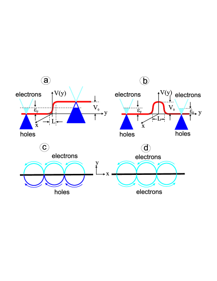
Figure 1: Schematic presentation of n-p and n-p-n junctions. Panels a and b show the potentials and the fillings the graohene bands while panels c and d show the classical orbits and the direction motion of electrons and holes skipping along the lateral junction.

II Dynamics of quasi-particles skipping along lateral junctions under magnetic field.

Let us consider semiclassical motion of a quasiparticle moving along p-n and n-p-n junctions under magnetic field as is shown in Fig.1 where panels a and b schematically present lateral electron-hole and electron-hole-electron junctions placed along the $x$-direction; panels c and d schematically show semiclassical orbits of electrons skipping along the lateral junctions, the arrow showing directions of the quasi-particle motion.

Quantum dynamics of quasi-particle (electrons and holes)in graphene with a lateral junction is described by the 2-component wave function $\Psi_{1,2}(x,y)$ satisfying the Schrödinger equation

$$\Big{(}V(y)-\varepsilon\big{)}\Psi_{1}+v\big{(}P_{x}+\frac{eH}{c}y-\hbar\frac{d}{dy}\Big{)}\Psi_{2}=0;$$

$$v\Big{(}P_{x}+\frac{eH}{c}y+\hbar\frac{d}{dy}\big{)}\Psi_{1}+\big{(}V(y)-\varepsilon\Big{)}\Psi_{2}=0;$$ (2)

where the vector potential ${\bf A}=(Hy,0,0)$ is used while $V(y)$ is the lateral barrier potential (of the n-p or n-p-n type, see Fig.1 ) extended along the $x$-direction. Here, the axis $x$ is parallel to the sample and the barrier junction while the $y$-axis is perpendicular to those as is shown in Fig.1; $P_{x}$ is the conserving projection of generalized momentum on the lateral junction direction.

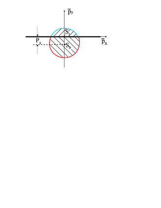
Figure 2: Areas of the semiclassical orbits in the momentum space at fixed conserving momentum projection $P_{x}$ for quasiparticles above and below the junction.

Taking semiclassical solutions of Eq.(2) above ($y>0$) and below ($y<1$) the lateral junction and matching them at the turning points and at the junction with the use of the $2\times 2$ scattering matrix one finds the proper wave functions and the quasiparticle spectrum.

I. The quasi-particle skipping along the p-n junction (see Fig.1a,c) is in a quantum superposition of the electron and hole edge states above ($y>0$) and below ($y<0$) the n-p junction:

$$\hat{\Psi}_{n,P_{x}}(x,y)=\left(\begin{matrix}\Psi_{1}\\ \Psi_{2}\end{matrix}\right)=e^{ixP_{x}/\hbar}\Big{(}\bar{C}_{e}\hat{\Psi}_{e,n,P_{x}}(y)\Theta(-y)\Big{)}$$

$$+\bar{C}_{h}\hat{\Psi}_{h,n,P_{x}}(y)\Theta(y)$$ (3)

where $n$ is the Landau number, $P_{x}$ is the conserving momentum projection to the lateral junctio and $\Theta(y)$ is the unit step function.

$\hat{\Psi}_{n,P_{x}}(x,y)$ are the proper wave functions of the Schrödinger equation Eq.(2), $\hat{\Psi}_{e}(y)$ and $\hat{\Psi}_{h}(y)$ are the semiclassical solutions of Eq.(2) at $y<0$ and $y>0$, respectively, the both of them being normalized to the unity flux while $|\bar{C}_{h}|^{2}+|\bar{C}_{e}|^{2}=1$.

According to Eq.(3), factors $|\bar{C}_{h}|^{2}$ and $|\bar{C}_{e}|^{2}$ are the probabilities to find the quasiparticle above the junction (that is in the hole state) and below it (that is in the electron state), respectively. As one easily sees from Eq.(44) and Eq.(52) these factors are fast oscillating functions of $P_{x}$ (on the $\hbar/R_{H}$ scale, $R_{H}$ being the Larmour radius of the quasiparticle cyclotron radius). Therefore, even a rather small change $\delta P_{x}\sim\hbar/R_{H}$ of the momenta $P_{x}$ greatly changes these probabilities and hence such a change sufficiently re-distributes the probabilities to find the quasiparticle above or below the junction.

After performing the above mentioned matching one finds the dispersion equation (which determines the qasiparticle spectrum $\varepsilon_{n}(P_{x})$) as follows:

$$D^{(eh)}\equiv\cos{\Phi_{-}^{(eh)}\left(\varepsilon,P_{x}\right)}-|r^{(eh)}|\cos{\Phi_{+}^{(eh)}(\varepsilon,P_{x})}=0;$$ (4)

where $\Phi_{+}^{(eh)}=(S_{e}+S_{h})/2\hbar$, $\Phi_{-}^{(eh)}=(S_{e}-S_{h})/2\hbar+\mu^{(eh)}$ while $S_{h}=2\int_{y_{e}}^{0}p_{e}dy$ and $S_{e}=2\int_{y_{e}}^{0}p_{e}dy$ are the areas of the hole and electron semiclassical orbits above and below the lateral barrier (see Fig.2 in which $S_{t}$ and $S_{b}$ schematically shows the hole and electron orbits, respectively), $r^{(eh)}=|r^{(eh)}|exp(i\mu^{(eh)})$ is the reflection probability amplitude at the junction; the turning points $y_{h,e}$ and the integrand momenta are

$$y_{h} = \frac{c}{eH}\left(\frac{V_{0}-\varepsilon}{v}-P_{x}\right);$$

$$p_{h}(y) = \sqrt{\left(\frac{V_{0}-\varepsilon}{v}\right)^{2}-\left(P_{x}+\frac{eH}{c}y\right)^{2}}$$

$$y_{e} = -\frac{c}{eH}\left(\frac{\varepsilon}{v}+P_{x}\right);$$

$$p_{e}(y) = \sqrt{\left(\frac{\varepsilon}{v}\right)^{2}-\left(P_{x}+\frac{eH}{c}y\right)^{2}}$$ (5)

At $\varepsilon\sim\varepsilon_{F}$ these phases are

$$\Phi_{\pm}\sim 1/\eta\gg 1,$$

$$\eta=\frac{\lambda_{F}}{R_{H}}=\frac{e\hbar H}{c}\Big{(}\frac{v}{\varepsilon_{F}}\Big{)}^{2}\ll 1$$ (6)

where $\eta$ is the semiclassical parameter, $\lambda_{F}=\hbar v/\varepsilon_{F}$ and $R_{H}=(c/eH)(\varepsilon/v)$ are the de Broglie wave length and the Larmour radius. The numerically calculated spectrum of quasiparticles $\varepsilon^{(eh)}_{n}(P_{x})$ skipping along the n-p interface is present in Fig.3, $n$ is the Landau number, $P_{x}$ is the conserving momentum projection.

The reflection probability at the n-p interface may be written as followsCastro :

$$|r^{(eh)}\big{(}\varepsilon,P_{x}\big{)}|^{2}=\frac{1-\sqrt{1-\big{(}vP_{x}/\varepsilon\big{)}^{2}}}{1+\sqrt{1-\big{(}vP_{x}/\varepsilon\big{)}^{2}}};\;V_{0}\gg\varepsilon_{F}$$ (7)

where $V_{0}$ is the height of the potential barrier (see Fig.1)

II. The electron skipping along the n-p-n junction (see Fig.1b,d), is also in a quantum superposition of the electron edge states above ($y>0$) and below ($y<0$) the junction analogous to Eq.(3). However, in contrast to the n-p junction the group velocity of the electron in the semiclassical states above and below the n-p-n junctions are of the opposite signs. As a results, the electron spectrum becomes gapped that determines peculiar properties of dynamics and kinetics of such electrons.

In the same way as it was done for quasiparticles skipping along the n-p junctions, matching the electronic semiclassical wave functions (See AppendixA) gives the following dispersion equation that determines the electron spectrum $\varepsilon_{n}^{(e)}(P_{x})$:

$$D^{(ee)}\equiv\cos{\Phi_{+}^{(ee)}\left(\varepsilon\right)}-r^{(ee)}(\varepsilon,P_{x})\cos{\Phi_{-}^{(ee)}\left(\varepsilon,P_{x}\right)}=0;$$ (8)

Here $\Phi_{\pm}=cS_{\pm}/2e\hbar H$ while $S_{\pm}=S_{1}\pm S_{2}$ and $S_{1}$ and $S_{2}$ are the areas of the semiclassical orbits above and below the lateral junction, respectively (see Fig.1). The sum and difference of the orbit areas $S_{\pm}=S_{1}\pm S_{2}$ are:

$$\Phi_{+}=\frac{\pi c}{2e\hbar H}\left(\frac{\varepsilon}{v}\right)^{2};$$

$$\Phi_{-}=\frac{c}{e\hbar H}\left(\frac{\varepsilon}{v}\right)^{2}\Big{\{}\frac{vP_{x}}{\varepsilon}\sqrt{1-\Big{(}\frac{vP_{x}}{\varepsilon}\Big{)}^{2}}$$

$$+\arcsin{\frac{\mu^{(ee)}P_{x}}{\varepsilon}}\Big{\}}+\mu^{(ee)}$$ (9)

Factor $|r^{(ee)}|^{2}$ is the probability of reflection at the n-p-n junction, $\mu^{(ee)}$ is the phase of its probability amplitude. For the sake of simplicity, one may use the reflection probability in the following formCastro :

$$r^{2}\left(P_{x}\right)=\frac{\lambda^{2}\left(vP_{x}/\varepsilon\right)^{2}}{1-\left(1-\lambda^{2}\right)\left(vP_{x}/\varepsilon\right)^{2}};\;\;\lambda=\frac{V_{0}L}{\hbar v}$$ (10)

which is valid at $\lambda\ll 1$. Here $V_{0}$ and $L$ are the height and the width of the potential $V(y)$ (see Fig.1). The numerically calculated spectrum of electrons $\varepsilon^{(ee)}_{n}(P_{x})$ skipping along the n-p-n interface is present in Fig.3, $n$ is the Landau number, $P_{x}$ is the conserving momentum projection.

Despite dispersion equations Eq.(4) and Eq.(8) look much alike they determine qualitatively different spectra: the former spectrum is gapless (see Fig.3A) while the latter one is gapped (see Fig.3B). As one readily sees from Eq.(8) the energy gaps are determined by the condition

$$|\cos{\Phi_{+}}(\varepsilon)|\geq|r^{(ee)}|;$$

On the other hand, one may get the necessary condition of solvability of Eq.(8) $|\cos{\Phi_{-}}(\varepsilon,P_{x})|<|r^{(eh)}|$ at any energy by varying $P_{x}$ that provides the gapless spectrum.

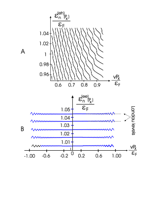
Figure 3: The spectrum of quasiparticles skipping along the n-p interface (panel A) and those skipping along the n-p-n interface (panel B) Numerical calculations are performed for the semiclassical parameter $\eta=10^{-2}$ and the n-p-n reflection probability parameter $\lambda=0.2$. The spectrum of the electrons skipping along the n-p-n junction is an alternating series of energy gaps and bands.

In order to explicitly calculate the density of states (DOS) it is convenient to use the approach developed by Slutskin for analogous spectra of electrons under magnetic breakdown conditions KaganovSlutskin . Below, calculations of DOS for the gapped spectrum Eq.(8) are presented.

Using Eq.(8) and the identity

$$\sum_{n}\delta(\varepsilon-\varepsilon_{n})=\Big{|}\frac{\partial D^{(ee)}}{\partial\varepsilon}\Big{|}\delta(D^{(ee)})$$ (11)

one transforms DOS

$$\nu(\varepsilon)=\frac{1}{2R_{H}}\sum_{n}\int_{-\varepsilon/v}^{\varepsilon/v}\delta\left[\varepsilon-\varepsilon_{n}(P_{x})\right]\frac{dP_{x}}{2\pi\hbar}$$ (12)

into the form

$$\nu(\varepsilon)=\frac{1}{2R_{H}}\sum_{n}\int_{-\varepsilon/v}^{\varepsilon/v}\Big{|}\frac{\partial D^{(ee)}}{\partial\varepsilon}\Big{|}\delta\left[D^{(ee)}\big{(}\varepsilon,P_{x}\big{)}\right]\frac{dP_{x}}{2\pi\hbar}$$ (13)

As one sees from Eq.(8) the integrand here is a $2\pi$-periodic function of $\Phi_{-}$ and hence it can be expanded into the Fourier series as follows:

$$\nu(\varepsilon)=\frac{1}{2R_{H}}\sum_{k=-\infty}^{\infty}\int_{-\varepsilon/v}^{\varepsilon/v}B_{k}\left(\varepsilon,P_{x}\right)e^{ik\Phi_{-}\left(\varepsilon,P_{x}\right)}\frac{dP_{x}}{2\pi\hbar}$$ (14)

where $B_{k}\left(\varepsilon,P_{x}\right)$ are amplitudes of the Fourier harmonics.

As at $\varepsilon\sim\varepsilon_{F}$ one has $\Phi_{-}\gg 1$ (see Eq.(6)) the exponents in Eq.(14) are fast oscillating functions while the Fourier coefficients are smooth functions of $P_{x}$ (on the scale $\hbar/R_{H}\ll p_{F}$). Therefore, the term with $k=0$ gives the main contribution to DOS:

$$\nu(\varepsilon)=\frac{1}{2R_{H}}\sum_{k=-\infty}^{\infty}\int_{-\varepsilon/v}^{\varepsilon/v}B_{0}\left(\varepsilon,P_{x}\right)\frac{dP_{x}}{2\pi\hbar}$$ (15)

where the Fourier factor $B_{k}$ at $k=0$ is

$$B_{0}=\int_{-\pi}^{\pi}\Big{|}\frac{\partial\Phi_{+}}{\partial\varepsilon}\sin{\Phi_{+}}-\frac{\partial\Phi_{-}}{\partial\varepsilon}\sin{\omega}\Big{|}$$

$$\times\delta\Big{[}\cos{\Phi_{+}(\varepsilon)}-|r^{(ee)}(P_{x})|\cos{\omega}\Big{]}\frac{d\omega}{2\pi}$$ (16)

While writing $B_{0}$ the explicit form of $D^{(ee)}$ (which is given by Eq.(8)) was used.

Carrying out integration in Eq.(16) and inserting the result in Eq.(15) one obtains DOS as follows:

$$\nu\left(\varepsilon\right) =\frac{\big{|}\sin{\Phi_{+}(\varepsilon)}\big{|}}{\hbar v}$$ (17)

$$\times \int_{-\varepsilon/v}^{\varepsilon/v}\frac{\Theta\Big{[}|r^{(ee)}|^{2}(P_{x})-\cos^{2}{\Phi_{+}(\varepsilon)}\Big{]}}{\sqrt{|r^{(ee)}|^{2}(P_{x})-\cos^{2}{\Phi_{+}(\varepsilon)}}}\frac{dP_{x}}{2\pi\hbar}$$

Here $\Theta[...]$ is the unit step function.

The result of numerical calculations of DOS with the use of Eq.(17) and Eq.(10) for the semiclassical parameter $\eta=10^{-2}$ and $\lambda=0.2$ is presented in Fig.4. As one sees in Fig.3 and Fig.4 the quantum interference of the edge states above and below the n-p-n junction (see Fig.1) results in arising of alternating series of energy gaps and energy bands which produce narrow peaks in the density of states. Fig.4B shows the density of states caused by the Zeeman splitting where $g$ is the gyromagnetic coefficient.

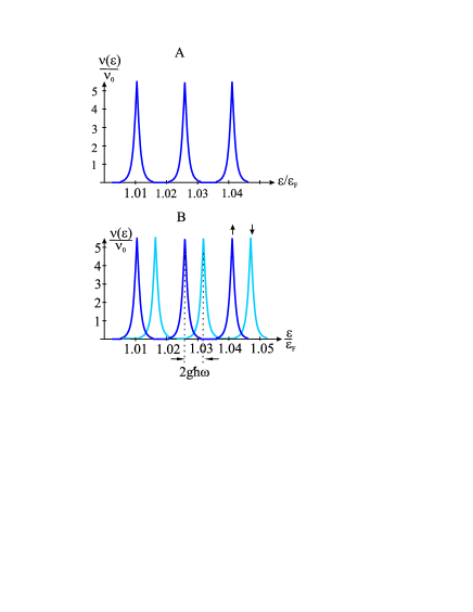
Figure 4: Density of states for electrons skipping along the n-p-n interface(panel A) normalized to the one in the absence of magnetic field $\nu_{0}=4\pi m/(2\pi\hbar)^{2}$. Panel B shows the Zeeman split of DOS. Numerical calculations are performed for the semiclassical parameter $\eta=10^{-2}$ and the n-p-n reflection probability parameter $\lambda=0.2$

Such a dramatic transformation of the quasi-particle spectrum has to show itself in various prominent effects in optic and kinetic properties. In the next section transport properties of both the clean and dirty graphene samples are analyzed.

III Current along p-n junction under magnetic field.

In this section the total current flowing inside the stripe $-2R_{H}^{(e)}\leq y2\leq R_{H}^{(h)}$ around the p-n junction is calculated where $R_{H}^{(e)}=(c/eH)(\varepsilon_{F}/v)$ and $R_{H}^{(h)}=(c/eH)((V_{0}-\varepsilon_{F})/v)$ are the Larmour radii of electrons (e) and holes (h);

It is easy to see that there are two types of quasiparticle states inside this stripe: they are states of quasiparticles which interact with the lateral junction that delocalized them in the junction direction, and those in which quasiparticles do not touch the junction (the Landau states - the quasiparticles move along closed semiclassical orbits). As only parts of the closed orbits are inside the stripe these quasiparticles create finite currents in the stripe below and above the junction. This situation is schematically shown in Fig.5.

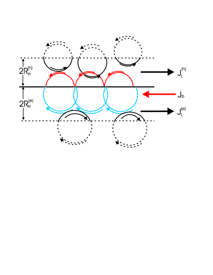
Figure 5: Schematic presentation of currents flowing in the vicinity of the n-p interface. Quasiparticles which are in the quantum electron-hole superposition are delocalized along the interface and carry current $J_{b}$ inside stripes of the widths $2R_{H}^{(h)}$ above the junction and $2R_{H}^{(e)}$ below the interface. Electrons and holes in the Landau states create currents $J_{L}^{(e)}$ and $J_{L}^{(h)}$ in the same stripes because only parts of their closed orbits are inside them. The later currents flow in the opposite direction to current $J_{b}$ exactly compensating it in the absence of the bias voltage.

In other words, the edge states partly replace the Landau states which would be inside the stripe in the absence of the junction that creates an imbalance between the Landau states. As a result, compensating currents of quasiparticles on closed orbits arise which flow in the opposite direction to the edge state current.

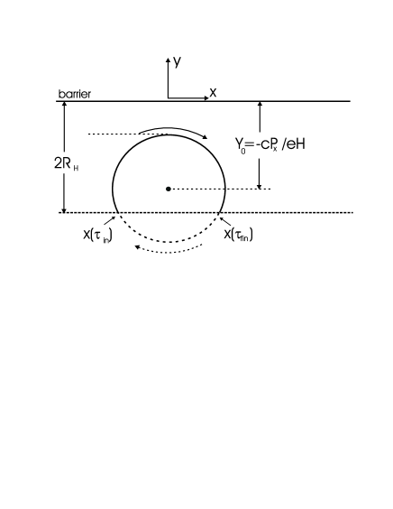
Figure 6: A semiclassical closed orbit of an electron in the Landau state. The electron moving along the part of the orbit inside the stripe of the width $2R_{H}^{(e)}$

at the junction (shown by solid line) contributes to the current flowing inside the stripe. $x(\tau_{in})$ and $x(\tau_{fin})$ are the initial and final x-coordinates of this motion.

Let us firstly calculate the current $J_{b}$ carried by quasiparticles in the edge states which flows from the right reservoir under bias voltage $V$ to the left one under voltage $V=0$. This current may be written as

$$J_{b}^{(eh)} = e\sum_{n}\int_{-\varepsilon^{(eh)}_{n}/v}^{\varepsilon_{n}/v}v_{x}\left(P_{x},\varepsilon^{(eh)}_{n}\left(P_{x}\right)\right)$$ (18)

$$\times f_{0}\Big{(}\varepsilon_{n}\left(P_{x}\right)+eV\Big{)}\frac{dP_{x}}{2\pi\hbar}$$

which may be re-written as

$$J_{b}^{(eh)} = e\int d\varepsilon f_{0}\left(\varepsilon+eV\right)\int_{-\varepsilon/v}^{\varepsilon/v}\frac{dP_{x}}{2\pi\hbar}$$ (19)

$$\times v_{x}\left(\varepsilon,P_{x}\right)\Big{|}\frac{\partial D^{(eh)}}{\partial\varepsilon}\Big{|}\delta\Big{[}D^{(eh)}\left(\varepsilon,P_{x}\right)\Big{]}$$

where $D^{(eh)}$ is defined in Eq.(4).

Using the same approach as in Subsection IV.1 one finds the current carried by quasiparticles delocalized along the p-n junction as follows:

$$J_{b}^{(eh)} = -\frac{c}{\pi\hbar H}\int d\varepsilon f_{0}\left(\varepsilon+eV\right)$$ (20)

$$\times \Big{\{}\int_{-\varepsilon/v}^{\varepsilon/v}\frac{dP_{x}}{2\pi\hbar}p_{y}^{(e)}+\int_{-(V_{0}-\varepsilon/v)}^{(V_{0}-\varepsilon)/v}\frac{dP_{x}}{2\pi\hbar}p_{y}^{(h)}\Big{\}};$$

Here $p_{y}^{(e,h)}$ are the $y$-projections of the electron and hole momenta inside the electron and hole parts of the electrically gated graphene in the absence of magnetic field:

$$p_{y}^{(e)} = \sqrt{\Big{(}\frac{\epsilon}{v}\Big{)}^{2}-P_{x}^{2}}$$

$$p_{y}^{(h)} = \sqrt{\Big{(}\frac{V_{0}-\epsilon}{v}\Big{)}^{2}-P_{x}^{2}}$$ (21)

As it follows from Eq.(20) the current of quasi-particles interacting with the junction does not depend on its transparency and is a sum of the electron and hole edge state currents flowing in the same direction. These edge state currents flows inside two stripes: $-2R_{H}^{(e)}<y<0$ and one $0<2R_{H}^{(h)}<y<0$.

As it was said above there are two other additional currents inside the same stripe around the junction flowing in the opposite direction to the current carried by the edge states Eq.(20).

Below, the current carried by electrons in the Landáu states inside the stripe $-2R_{H}^{(e)}<y<0$ is calculated.

The current density is written as follows:

$$j_{L}^{(e)}(\textbf{r}_{0})=eTr\Big{\{}\delta(\hat{\textbf{r}}-\textbf{r}_{0})f_{0}\big{(}\hat{{\cal H}_{0}}\big{)}\hat{v}_{x}$$

$$+f_{0}\big{(}\hat{{\cal H}_{0}}\big{)}\hat{v}_{x}\delta(\hat{\textbf{r}}-\textbf{r}_{0})\Big{\}}$$ (22)

where the velocity operator $\hat{v}_{x}$ is

$$\hat{v}_{x}=\frac{i}{\hbar}\left[\hat{{\cal H}}_{0},\hat{x}\right]$$ (23)

and $\hat{{\cal H}}_{0}$ is the Hamiltonian corresponding to the Schrödinger equation Eq.(2) in the absence of the junction, $V(y)\equiv 0$.

Using Eq.(22) one finds the current inside the stripe in the semiclassical approximation as follows:

$$J_{L}^{(e)}=e\int_{\varepsilon/v}^{3\varepsilon/v}\frac{dP_{x}}{2\pi\hbar}\int\frac{dP_{y}}{2\pi\hbar}\int_{-2\widetilde{R}^{(e)}_{H}}^{y_{1}}dy$$

$$\times f_{0}\Big{[}{\cal H}_{0}(P_{x}+\frac{eH}{c}y,P_{y})\Big{]}v_{x}\Big{[}{\cal H}_{0}(P_{x}+\frac{eH}{c}y,P_{y})\Big{]};$$ (24)

Here the argument of the Fermi distribution function $f_{0}$ is the classical Hamiltonian of the graphene under magnetic field while ${\cal H}_{0}(\textbf{p})=v\sqrt{p_{x}^{2}+p_{y}^{2}}$ is the classical Hamiltonian of graphene at $H=0$ and $P_{x},P_{y}$ are the projections of the electron generalized momentum; $y_{1}=-cP_{x}/eH+R_{H}^{(e)}$ is the turning point nearest to the junction, $R_{H}^{(e)}=(c/eH)(\varepsilon/v)$ is the Larmour radius at fixed electron energy $\varepsilon$; the limits of integration with respect to $P_{x}$ are determined by the condition that the turning point $y_{1}$ is inside the stripe, $-2\widetilde{R}^{(e)}_{H}\leq y_{1}\leq 0$.

It is convenient to insert new variables $P_{x},P_{y}\rightarrow\varepsilon,\tau$ where $\tau$ is the time of motion along the classical electron orbit. In this variables the equation of electron motion under magnetic field is the standard Hamilton equation:

$$\frac{d\textbf{p}}{d\tau}=\frac{e}{c}\Big{[}\textbf{v}\times\textbf{H}\Big{]}$$ (25)

where $\textbf{p}=(P_{x}+(eH/c)y,P_{y})$.

Inserting the new variables in Eq.(24) and using Eq.(25) one finds the current of the Landau electrons inside the stripe as follows:

$$J_{L}^{(e)}=\frac{e}{(2\pi\hbar)^{2}}\frac{c}{eH}\int_{\varepsilon/v}^{3\varepsilon/v}dP_{x}$$

$$\int d\varepsilon f_{0}(\varepsilon)\left(p_{y}(\tau_{in})-p_{y}(\tau_{fin})\right)$$ (26)

where $p_{y}(\tau)=-(eH/c)x(\tau)$ according to Eq.(25) and $x(\tau_{in,fin})$ are the initial and final $x$-coordinates of motion of the electron along its orbit (see Fig.6). It is easy to see that

$$p_{y}(\tau_{fin})=-p_{y}(\tau_{in})=\sqrt{\left(\frac{\varepsilon}{v}\right)^{2}-\left(P_{x}-2\frac{\varepsilon}{v}\right)^{2}};$$

Inserting this equation in Eq.(26) one finally finds the current of electrons in the Landau state inside the stripe $-2R_{H}^{(e)}\leq y\leq 0$ as follows:

$$J_{L}^{(e)}=\frac{c}{\pi\hbar H}\int d\varepsilon f_{0}\left(\varepsilon\right)\int_{-\varepsilon/v}^{\varepsilon/v}\frac{dP_{x}}{2\pi\hbar}\sqrt{\left(\frac{\varepsilon}{v}\right)^{2}-P_{x}^{2}};$$ (27)

Performing analogous calculations for the current $J_{L}^{h}$ carried by holes in Landau states inside the stripe $0\leq y\leq 2R_{H}^{(h)}$ one gets

$$J_{L}^{(h)} = \frac{c}{\pi\hbar H}\int d\varepsilon f_{0}\left(\varepsilon+eV\right)$$ (28)

$$\times \int_{-(V_{0}-\varepsilon/v)}^{(V_{0}-\varepsilon)/v}\frac{dP_{x}}{2\pi\hbar}\sqrt{\Big{(}\frac{V_{0}-\epsilon}{v}\Big{)}^{2}-P_{x}^{2}};$$

Comparing Eq.(27) and Eq.(28) with Eq.(20) one sees that the currents of quasiparticles in the Landau states $J^{(e,h)}_{L}$ and the one carried by electrons in the edge states , $J_{b}^{(eh)}$, flow in the opposite directions being modulo equal in the absence of the bias voltage, $V=0$.

Summing the currents given by Eq.(20,27,28) and expanding the Fermi function with respect to $eV/kT\ll 1$ one finds the total current $J_{total}^{(eh)}=J_{b}^{(eh)}+J_{L}^{(e)}+J_{L}^{(h)}$ flowing inside the stripe $-2R_{H}^{(e)}\leq y\leq 2R_{H}^{(h)}$ biased by the voltage drop $V$ as follows:

$$J_{total}^{(eh)} = -\frac{ec}{\pi\hbar H}\int d\varepsilon\frac{df_{0}(\varepsilon)}{d\varepsilon}\Big{\{}\int_{-\varepsilon/v}^{\varepsilon/v}\frac{dP_{x}}{2\pi\hbar}\sqrt{\Big{(}\frac{\epsilon}{v}\Big{)}^{2}-P_{x}^{2}}$$ (29)

$$+ \int_{-(V_{0}-\varepsilon/v)}^{(V_{0}-\varepsilon)/v}\frac{dP_{x}}{2\pi\hbar}\sqrt{\Big{(}\frac{V_{0}-\epsilon}{v}\Big{)}^{2}-P_{x}^{2}}\Big{\}}V;$$

Therefore, one sees that the current flowing along the p-n junction $J_{total}^{(eh)}$ is a sum of the standard edge state of currents of separated electrons and holes at the separated sample borders. As it follows from Eq.(29) the value of the current $J_{total}^{(eh)}$ does not depend on the sign of the applied voltage drop $V$.

In conclusion of the section, the current flowing along the p-n junction is inevitably the sum of two qualitatively different types of the currents:

1) the current carried by quasiparticles which are a quantum superposition of electron and hole states; these states are delocalized along the lateral junction and quasiparticles in those states create current $J_{b}^{(eh)}$ (see Eqs.(4), 20).

2) Currents of electrons and holes in the Landau states which do not interact with the p-n junction. Such quasiparticles move along closed semiclassical orbits, only parts of those orbits being inside the above-mentioned stripe. They create electron and hole currents $J_{L}^{(e)}$ and $J_{L}^{(h)}$.

As one easy sees these currents flow in the opposite direction to the current $J_{b}^{(eh)}$ compensating the latter if $V=0$ (see Eqs.(20,27,28)). This statement is correct in the lowest semiclassical approximation in which all the three currents have been obtained. In quantum oscillating corrections to the smooth part of the currents considered here, as well as in the quantum Hall regime (in which dynamics and kinetics of quasiparticles are of the fundamentally quantum character) the above-mentioned compensation is absent because of the different quantum behavior of electrons in the Landau states and those delocalized along the junction. As the quasiparticles in such a situation are in the essentially quantum states it seems doubtful whether arising of the oscillations is a manifestation of the semiclassical snake-like trajectories (snake states)Carmier ; Beenakker . Note that peculiar conductance oscillations were observed in samples of high qualityThiti ; Rickhaus , the latter condition being one of the necessary conditions for observation of quantum effects.

IV Giant oscillations of the conductance of grphene ribbon with n-p-n lateral junction under magnetic field.

IV.1 Ballistic transport

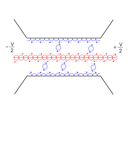
Figure 7: Schematic presentation of the graphene ribbon with a lateral n-p-n junction biased by voltage V under magnetic field.

In this section the ballistic transport through a graphene ribbon with an n-p-n junction under magnetic field is considered.

The sample is schematically shown in Fig.7. As one sees there are two qualitatively different types of currents flowing along the sample: current $J^{(ee)}_{edge}$ carried by electrons edge states at the external sample boundaries and current $J_{b}$ carried by electrons localized along the n-p-n junction the dispersion equation of which is given by Eq.(8) (their spectrum is presented in Fig.3B)

According to the Landauer-Büttiker approach, based on the relationship between the conductance and the transmission probability in propagating channels, Dittrich the linear conductance may be written as follows:

$$G = \frac{2e^{2}}{kT}\sum_{n}\int_{-\varepsilon/v}^{\varepsilon/v}\frac{dP_{x}}{2\pi\hbar}\Big{|}v^{(ee)}_{x}\left[\varepsilon^{(ee)}_{n}(P_{x}),P_{x}\right]\Big{|}$$ (30)

$$\times \cosh^{-2}\frac{\varepsilon^{(ee)}_{n}(P_{x})-\varepsilon_{F}}{2kT};$$

where the quasiparticle velocity is $v^{(ee)}_{x}=d\varepsilon^{(ee)}_{n}/dP_{x}$

In the analogous way as deriving DOS, Eq.(12), one gets the conductance along then-p-n lateral junction as follows (details of calculations are presented in Appendix B):

$$\frac{G_{b}\left(H\right)}{G_{edge}}=\frac{4}{\pi}\sum_{n}\int_{-1}^{1}dq\sqrt{1-q^{2}}$$

$$\Big{(}\tanh\frac{\varepsilon_{n}^{(t)}-\varepsilon_{F}}{2kT}-\tanh\frac{\varepsilon_{n}^{(b)}-\varepsilon_{F}}{2kT}\Big{)}$$ (31)

where $G_{edge}=G_{0}(2R_{H}/\lambda_{F})$ is the conductance of the edge states in the graphene ribbon in the absence of the lateral junction, $G_{0}=e^{2}/h$ is the conductance quant and $2R_{H}/\lambda_{F}$is the number of the propagating channels of the edge states; $\lambda_{F}=\hbar/p_{F}$ while $\varepsilon_{n}^{(b,t)}(H)$ are the bottom and the top of the $n$-th electron energy band which are found from the condition $\cos{\Phi_{+}}(\varepsilon)=|r(P_{x})|$ (see Eq.(8)):

$$\varepsilon_{n}^{(b,t)}(H) = v\sqrt{\frac{e\hbar H}{c}}\sqrt{2n+1}$$ (32)

$$\pm \frac{v^{2}}{2\varepsilon_{F}}\frac{e\hbar H}{c}\Big{(}1-\frac{2}{\pi}\arccos{|r(P_{x})|}\Big{)}$$

The dependance of the conductance along the n-p-n junction on magnetic filed is shown in Fig.8.

Figure 8: Conductance oscillations with variations of the magnetic field; $G_{edge}=(e^{2}/h)(2R_{h}/\lambda_{F})$ is the conductance of edge states in the graphene ribbon in the absence of the lateral junction. Numerical calculations are performed for the semiclassical parameter $\eta=10^{-2}$ and the n-p-n reflection probability parameter $\lambda=0.2$.

Giant oscillation of the conductance at a fixed magnetic field $H$ may be observed if the chemical potential is varied together with the gate potential $V_{g}$. In this case the conductance is determined by Eq.(31) in which $\varepsilon_{F}$ is changed to $\varepsilon_{F}+eV_{g}$. This dependence of the conductance on the gate potential is presented in Fig.9.

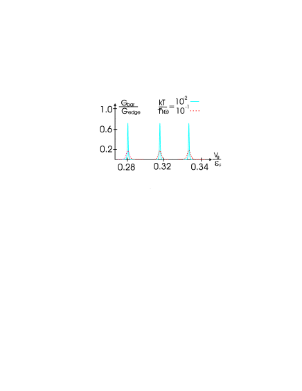
Figure 9: Conductance oscillations with variations of the gate voltage $V_{g}$; $G_{edge}=(e^{2}/h)(2R_{h}/\lambda_{F})$ is the conductance of edge states in the graphene ribbon in the absence of the lateral junction. Numerical calculations are performed for the semiclassical parameter $\eta=10^{-2}$ and the n-p-n reflection probability parameter $\lambda=0.2$.

The total current flowing along a graphene ribbon with an e-h-e lateral junction (see Fig.7) is $J_{total}=J_{bar}+2J_{edge}$ where $J_{bar}$ is the current carried by electrons skipping along the junction and $2J_{edge}$ are the edge state currents. This current may be written as $J_{total}=V/R_{total}$ where $R_{total}$ is the total resistance of the ribbon. For a ribbon with $N$ parallel lateral junctions its total resistance is

$$R_{total}=\frac{1}{G_{edge}+NG_{b}}$$ (33)

This equation is written under assumption that the distance between the junctions $L_{b}>2R^{(ee)}_{H}$ and the width of the ribbon $W>2R^{(ee)}_{H}N$. Numerical calculations of the total resistance $R_{total}$ for $N=1$ with the use of Eq.(31) is presented in Fig.10.

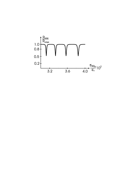
Figure 10: Total resistance of a graphene ribbon with one n-p-n interface under magnetic field. $R_{edge}$ is the resistance of the graphene ribbon in the absence of the lateral junction. An extremely small change of the magnetic field (or the voltage gate) may controllably cause the 50% change of the total ribbon resistance.Numerical calculations are performed for the semiclassical parameter $\eta=10^{-2}$ and the n-p-n reflection probability parameter $\lambda=0.2$.

As one sees from Eqs.(8,33) and Fig.10 a variation of the magnetic field $\delta H/H\approx 10^{-1}\hbar\omega_{H}/\varepsilon_{F}\ll 1$ produces a 50% jump of the total resistance of the ribbon with one lateral junction. As one readily sees the resistance jump for the ribbon with $N$ lateral junctions is

$$\frac{R_{total}^{(max)}-R_{total}^{(min)}}{R_{total}^{(max)}}=\frac{N}{(N+1}$$ (34)

that allows to have the giant magnetoresistance controlled be small variation of either the magnetic field or the gate voltage (here $R_{total}^{max,min}$ are the maximal and minimal values of the total resistance. For $N=3$, e.g., the jump is 75% of the total resistance. This property of such electrically gated graphene ribbons may be useful in modelling of devices based on the giant magnetoresistance effects of other types.

In the next subsection the current flowing along a graphene ribbon with a lateral n-p-n junction under magnetic field and in the presence of impurities is considered.

IV.2 Dissipative transport.

As in the case of the magnetic breakdown phenomenon, dynamic and kinetic properties of quasi-particles skipping along the junction under magnetic field are of the fundamentally quantum mechanical nature due to the quantum interference of their wave functions with semiclassically large phases. Thus, in order to analyze the transport properties of the quasi-particles in the presence of impurities it is convenient to start with the the equation for the density matrix $\hat{\rho}$ in the $\tau$ approximation:

$$\frac{i}{\hbar}\Big{[}\hat{\rho},\hat{H_{0}}\Big{]}-\frac{i}{\hbar}\Big{[}\hat{\rho},e{\cal E}\hat{x}\Big{]}+\frac{\hat{\rho}-f_{0}(H)}{t_{0}}=0;$$ (35)

Here, $\hat{H}$ is the Hamiltonian corresponding to the Schr odinger equation Eq.(2), $f_{0}$ is the Fermi distribution function, ${\cal E}$ is the electric field along the junction, $t_{0}$ is the electron scattering time.

Writing the density matrix in the form $\hat{\rho}=f_{0}(\hat{H})+\hat{\rho}^{(1)}$ and linearizing Eq.(35) with respect to the electric field one gets

$$\frac{i}{\hbar}\Big{[}\hat{\rho}^{(1)},\hat{H_{0}}\Big{]}+\frac{\hat{\rho}^{(1)}}{t_{0}}=-e{\cal E}\hat{v}_{x}f_{0}^{\prime}(\hat{H});$$ (36)

where $\hat{v}_{x}$ is the quantum mechanical operator of the quasi-particle velocity projection on the electric field direction, $f_{0}^{\prime}(\varepsilon)=df(\varepsilon)/d\varepsilon$.

In terms of the density matrix the current carried by the electrons skipping along the junction is written as follows:

$$J=2eTr\left\{\hat{v}_{x}\hat{\rho}\right\}$$ (37)

Taking the matrix elements of equation Eq.(36) with respect to proper functions of Schrödinger equation Eq.(2) written in the Dirac notations

$$\hat{H}\left|\kappa\right\rangle=\varepsilon_{\kappa}\left|\kappa\right\rangle;$$ (38)

(here $\kappa=\{n,P_{x}\}$) one finds the density matrix. Inserting the found solution in Eq.(37) one obtains the current $J$ as follows:

$$J=-e^{2}{\cal E}\sum_{\kappa,\bar{\kappa}}\frac{\partial f_{0}}{\partial\varepsilon}\Big{|}_{\varepsilon=\varepsilon_{\kappa}}\frac{\hbar\big{|}v_{\kappa,\bar{\kappa}}\big{|}^{2}}{i\big{(}\varepsilon_{\kappa}-\varepsilon_{\bar{\kappa}}\big{)}+\hbar\nu_{0}}$$ (39)

where $\sum_{\kappa}=\sum_{n}\int dP_{x}/2\pi\hbar$ while $v_{\kappa,\bar{\kappa}}=<\bar{\kappa}|\hat{v}_{x}|\kappa>$ and $\nu_{0}=1/t_{0}$ is the electron-impurity relaxation frequency.

As follows from Eq.(8)(see also Fig.3B) the distance between energy levels $\big{|}\varepsilon_{\kappa}-\varepsilon_{\bar{\kappa}}\big{|}\sim\hbar\omega_{H}$ and hence for the case considered below $\omega_{H}\gg\nu_{0}$ the main contribution to the sum is of the diagonal elements because the diagonal element $v_{\kappa,\kappa}\neq 0$ for delocalized quasi-particles. From here it follows that the current along the junction may written as

$$J=-e^{2}{\cal E}t_{0}\sum_{n}\int_{-\varepsilon_{F}/v}^{\varepsilon_{F}/v}\frac{dP_{x}}{2\pi\hbar}\big{|}v^{(ee)}_{n}(P_{x})\big{|}^{2}\frac{\partial f_{0}}{\partial\varepsilon}\Big{|}_{\varepsilon=\varepsilon^{(ee)}_{n}(P_{x})}$$ (40)

where $v^{(ee)}_{n}(P_{x})\equiv v_{\kappa,\kappa}=d\varepsilon^{(ee)}_{n}(P_{x})/dP_{x}$.

Using the same approach as in Subsection IV.1 one finds the conductance along the n-p-n junction in the presence of impurities as follows:

$$\frac{G_{dirty}}{G_{Drude}}=-8\int d\varepsilon\frac{\partial f_{0}(\varepsilon-eV_{g})}{\partial\varepsilon}\Big{|}\sin{\Phi_{+}(\varepsilon)}\Big{|}\int_{-1}^{1}d\xi$$

$$\frac{(1-\xi^{2})\sqrt{r^{2}(\xi)-\cos^{2}{\Phi_{+}(\varepsilon)}}\theta\Big{[}|r^{(ee)}|^{2}(\xi)-\cos^{2}{\Phi_{+}(\varepsilon)}\Big{]}}{\pi^{2}\sin^{2}{\Phi_{+}(\varepsilon)}-\big{(}|r^{(ee)}|^{2}(\xi)-\cos^{2}{\Phi_{+}(\varepsilon)\big{)}}\big{(}2\arcsin{\xi}\big{)}^{2}};$$ (41)

where $G_{Drude}=\sigma_{0}R_{H}$. Here $\sigma_{0}=\varepsilon_{F}e^{2}t_{0}/\hbar^{2}$ is the Drude conductivity of graphene in the absence of magnetic field, $H=0$.

Dependence of the conductance on the gate voltage $V_{g}$ in the presence of impurities is presented in Fig.11. As one sees the conductivity $G_{dirty}/R_{H}$ reaches the Drude conductivity when the energy $\varepsilon_{F}+eV_{g}$ is in the middle of a band and is equal to zero when it is inside a gap of the energy spectrum (see Fig.3B).

The above giant oscillations of the conductance are based on the quantum interference of the edge states on the both sides of the lateral n-p-n junctions that transforms the gapless spectra of the separated edge states into a series of alternating energy gaps and bands. In the same way as it takes place for magnetic breakdown this pure quantum mechanical picture holds if the path traversed by the "new" quasiparticle between collisions is greater than the individual classical trafectory Lifshitz . It means that in the case under consideration the bands give the main contribution to the conductance if the following inequality holds:

$$<v_{gr}>t_{0}\gg R_{H}^{(e)}$$ (42)

where $<...>=\int_{0}^{p_{F}}(...)dP_{x}/p_{F}$, the group velocity $v_{gr}=|r^{(ee)}(P_{x})|d\varepsilon^{(ee)}_{n}/dP_{x}$ and $t_{0}$ is the free path time, $|r(P_{x})|$ is the probability amplitude of the reflection at the n-p-n junction. This inequality may be re-written as

$$<|r^{(ee)}(P_{x})|>\gg\frac{R_{H}}{l_{0}}$$ (43)

where $l_{0}=vt_{o}$ is the free path length.

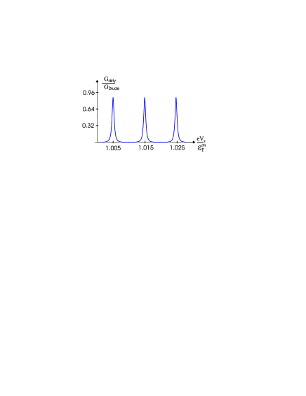
Figure 11: Giant oscillations of the conductance of a dirty graphene ribbon with an n-p-n interface under variations of the gate voltage $V_{g}$ normalized to $G_{Drude}=\sigma R_{H}^{(e)}$. Numerical calculations are performed for the semiclassical parameter $\eta=10^{-2}$ and the n-p-n reflection probability parameter $\lambda=0.2$.

V Discussion and Conclusion.

Quantum dynamics and kinetics of quasipartcles in a graphene ribbons with either n-p or n-p-n lateral interface under magnetic field is considered in the semiclassical approximation. Calculations of the current flowing along the n-p junction in the voltage biased ribbon show that there are three different currents inside the regions $-2R_{H}^{(e)}\leq y<0$ and $0<y\leq 2R_{H}^{(h)}$ around the lateral junction at $y=0$ (see Fig.5). One of them is the current of the quasiparticles skipping along the interface, $J_{b}^{(eh)}$, (see Eq.(20)). The other two are currents $J_{L}^{(e)}$ and $J_{L}^{(h)}$ which are created by quasiparticles in the localized Landau states the closed orbits of which are partially inside the above-mentioned regions around the n-p lateral junction (see Eqs.(27,28). The latter currents flow in the opposite direction to the current of the skipping quasiparticles $J_{b}^{(eh)}$ exactly compensating it in the absence of the bias voltage. As a result, the measurable current (which is the sum of those three currents) flowing along the biased n-p junction is the sum of two standard edge state currents of electrons and holes independently flowing along the junction (see Eq.(29)). Therefore, the snake-like states suggested in Ref.Beenakker do not manifest themselves in the main smooth part of the conductance of a graphene ribbon with an n-p interface. In principle, the snake-like states could implicitly affect the quantum oscillating corrections or the conductance in the regime of the quantum Hall effect but the essentially quantum character of the latter contradicts the classical nature of the former.

It is also shown that giant conductance oscillations may arise in a biased graphene ribbon with an n-p-n lateral interface under magnetic field. In such a state of the ribbon, depending on the number of n-p-n interfaces inside the ribbon, its total magnetoresistance may be controllably changed by $50\%\div 90\%$ by an extremely small variation of the gate voltage or the magnetic field (see Fig.10 and Eq.(34))

Appendix A Dispersion equation for quasiparticles skipping along an n-p junction under magnetic field.

The semiclassical solutions of Eq.(2) above and below the junction ($0<y<y_{h}$ and $y_{e}<y<0$, respectively) are

$$\widehat{\Psi}_{h} =\frac{C_{h}}{(y_{t}-y)^{(}1/4)}$$ (44)

$$\times \Big{[}\left(\begin{matrix}1\\ -e^{-i\varphi_{h}}\end{matrix}\right)\exp\left\{\frac{i}{\hbar}\int_{y}^{y_{h}}p_{h}(y^{\prime})dy^{\prime})-\frac{\pi}{4}\right\}+h.c.\Big{]},$$

$$\widehat{\Psi}_{e} =\frac{C_{e}}{(y_{t}-y)^{(}1/4)}$$

$$\times \Big{[}\left(\begin{matrix}1\\ -e^{-i\varphi_{e}}\end{matrix}\right)\exp\left\{\frac{i}{\hbar}\int_{y_{e}}^{y}p_{e}(y^{\prime})dy^{\prime})-\frac{\pi}{4}\right\}+h.c.\Big{]}$$

where

$$y_{h} = \frac{c}{eH}\left(\frac{V_{0}-\varepsilon}{v}-P_{x}\right);\varphi=\arctan\frac{p_{h}(y)}{P_{x}+eHy/c}$$

$$p_{h}(y) = \sqrt{\left(\frac{V_{0}-\varepsilon}{v}\right)^{2}-\left(P_{x}+\frac{eH}{c}y\right)^{2}}$$

$$y_{e} = -\frac{c}{eH}\left(\frac{\varepsilon}{v}+P_{x}\right);\varphi_{e}=\arctan\frac{p_{e}(y)}{P_{x}+eHy/c}$$

$$p_{e}(y) = \sqrt{\left(\frac{\varepsilon}{v}\right)^{2}-\left(P_{x}+\frac{eH}{c}y\right)^{2}}$$ (45)

are the turning points while $P_{x}$ is the conserving generalized momentum.

The constants $C_{h}$ and $C_{e}$ are determined by the matching of the above wave functions at the lateral junction and by the normalization condition.

In order to match the wave functions at the junction, $y=0$, it is convenient to write the integrals in Eq. (44) as $\int_{y}^{y_{t},y_{b}}(...)dy^{\prime}\approx\int_{0}^{y_{t},y_{b}}(...)dy^{\prime}+\int_{y}^{0}...dy^{\prime})$. After expanding the latter integrals in $|y|/R_{H}\ll 1$ one gets

$$\int_{y}^{y_{h}}p_{h}(y^{\prime})\frac{dy^{\prime}}{\hbar}\approx\frac{S_{h}}{e\hbar H/c}-\frac{yp_{h}(0)}{\hbar},$$

$$\int_{y_{e}}^{y}p_{e}(y^{\prime})\frac{dy^{\prime}}{\hbar}\approx\frac{S_{b}}{e\hbar H/c}+\frac{yp_{e}(0)}{\hbar}$$ (46)

where

$$S_{h}=\int_{0}^{(V_{0}-\varepsilon/v-P_{x})}\sqrt{\left(\frac{V_{0}-\varepsilon}{v}\right)^{2}-\left(P_{x}+\overline{p}_{x}\right)^{2}}d\overline{p}_{x},$$

$$S_{e}=\int^{0}_{-(\varepsilon/v+P_{x})}\sqrt{\left(\frac{\varepsilon}{v}\right)^{2}-\left(P_{x}+\overline{p}_{x}\right)^{2}}d\overline{p}_{x}$$ (47)

are the areas of the semiclassical orbits in the momentum space shown in Fig.2 in which $\overline{p}_{y}=\sqrt{(\varepsilon/v)^{2}-\left(P_{x}+\overline{p}_{x}\right)^{2}}$

As one easily sees from Eq.(44) and Eq.(46), in the vicinity of the junction $|y|\ll R_{H}$ the wave functions in Eq. (44) are plane waves:

$$\widehat{\Psi}_{h}=\frac{1}{p_{h}(0)}$$

$$\times\left(\begin{matrix}1\\ -e^{-i\varphi_{h}}\end{matrix}\right)\Big{[}A_{h}\exp\left\{ip_{h}(0)y/\hbar\right\}+B_{h}\exp\left\{-ip_{h}(0)y/\hbar\right\}\Big{]},$$

$$\widehat{\Psi}_{e}=\frac{1}{p_{e}(0)}$$

$$\left(\begin{matrix}1\\ -e^{-i\varphi_{e}}\end{matrix}\right)\Big{[}A_{e}\exp\left\{ip_{e}(0)y/\hbar\right\}+B_{e}\exp\left\{-ip_{e}(0)y/\hbar\right\}\Big{]}$$ (48)

Here the constants at the plane waves are

$$A_{h}=C_{h}\exp\{i\big{(}\frac{S_{h}}{e\hbar H/c}+\frac{\varphi_{h}(0)}{2}-\frac{\pi}{4}\big{)}\}$$

$$B_{h}=C_{h}\exp\{-i\big{(}\frac{S_{h}}{e\hbar H/c}+\frac{\varphi_{h}(0)}{2}-\frac{\pi}{4}\big{)}\}$$

$$A_{e}=C_{e}\exp\{i\big{(}\frac{S_{e}}{e\hbar H/c}-\frac{\varphi_{h}(0)}{2}-\frac{\pi}{4}\big{)}\}$$

$$B_{e}=C_{e}\exp\{-i\big{(}\frac{S_{h}}{e\hbar H/c}-\frac{\varphi_{e}(0)}{2}-\frac{\pi}{4}\big{)}\}$$ (49)

The incoming quasiparticle undergoes the two-channel scattering at the n-p junction and hence the constant factors at the scattered plain waves are matched with a $2\times 2$ scattering unitary matrix which is written in the general case as

$$\hat{\tau}^{(eh)}=\left(\begin{matrix}t^{(eh)}&r^{(eh)}\\ -r^{(eh)\ast}&t^{(eh\ast)}\end{matrix}\right),$$ (50)

where $t^{(eh)}$ and $r^{(eh)}$ are the probability amplitudes for the incoming quasiparticle to pass through and to be scattered back at the n-p junction, respectively, $|t^{(eh)}|^{2}+|r^{(eh)}|^{2}=1$.

Using Eqs.48 and Eq.(50) one matches the factor at the plain waves as follows:

$$B_{e}=\left(r^{(eh)}A_{e}+t^{(eh)}A_{h}\right)$$

$$B_{h}=\left(-t^{(eh)\ast}A_{e}+r^{(eh)\ast}A_{h}\right)$$ (51)

Replacing $A_{e,h}$ and $B_{e,h}$ by $C_{e,h}$ with the usage of Eq.(49) one finds a $2\times 2$ set of homogeneous linear algebraic equations for the required constant factors $C_{e,h}$ at the semiclassical wave functions Eq.(44):

$$\left(e^{-i\theta_{e}}-r^{(eh)}e^{i\theta_{e}}\right)C_{e}-t^{(eh)}e^{-i\theta_{h}}C_{h}=0;$$

$$t^{(eh)\ast}e^{i\theta_{e}}C_{e}+\left(e^{i\theta_{h}}-r^{(eh)\ast}e^{-i\theta_{h}}\right)C_{h}=0;$$ (52)

where

$$\theta_{e}=\frac{1}{\hbar}\int_{y_{e}}^{0}p_{e}dy;\;\;\;\theta_{e}=\frac{1}{\hbar}\int_{y_{e}}^{0}p_{e}dy;$$ (53)

Equating the determinant of equation Eq.52 to zero one finds the dispersion equation Eq.(4) of the main text.

Appendix B Derivation of the conductance of pure graphene with n-p-n interface.

It is convenient to re-write Eq.(30) as follows:

$$G = \frac{2e^{2}}{kT}\int_{-\infty}^{\infty}d\varepsilon\int_{-\varepsilon/v}^{\varepsilon/v}\frac{dP_{x}}{2\pi\hbar}\cosh^{-2}\big{[}\frac{\varepsilon-\varepsilon_{F}}{2kT}\big{]}$$ (54)

$$\times \Big{|}v^{(ee)}_{x}\left(\varepsilon,P_{x}\right)\Big{|}\sum_{n}\delta\big{[}\varepsilon-\varepsilon^{(ee)}_{n}(P_{x})\big{]};$$

Using Slutskin’s approach (see the derivation of Eq.(17) and the equation

$$v^{(ee)}_{x}=-\frac{\partial D^{(ee)}}{\partial P_{x}}\Big{/}\frac{\partial D^{(ee)}}{\partial\varepsilon}$$ (55)

one gets

$$G = \frac{2e^{2}}{kT}\int d\varepsilon\cosh^{-2}\big{[}\frac{\varepsilon-\varepsilon_{F}}{2kT}\big{]}$$ (56)

$$\times \int\frac{dP_{x}}{2\pi\hbar}\Big{|}\frac{\partial D^{(ee)}}{\partial P_{x}}\Big{|}\delta\Big{[}D^{(ee)}\left(\varepsilon,P_{x}\right)\Big{]}$$

Inserting the explicit expression for $D^{(ee)}$ (see Eq.(8)) in the integrand one finds

$$G=\frac{2e^{2}}{kT}\int d\varepsilon\cosh^{-2}\big{[}\frac{\varepsilon-\varepsilon_{F}}{2kT}\big{]}\int\frac{dP_{x}}{2\pi\hbar}$$

$$\Big{|}r^{(ee)}\Big{|}\Big{|}\sin{\Phi_{-}^{(ee)}}\Big{|}\sqrt{\big{(}\frac{\varepsilon}{v}\big{)}^{2}-P_{x}^{2}}$$

$$\delta\Big{[}\cos{\Phi_{+}^{(ee)}}-r^{(ee)}\cos{\Phi_{-}^{(ee)}}\Big{]}$$ (57)

Expanding the integrand into the Fourier series in $\Phi_{-}$ and taking the zero harmonics of it (which gives the main contribution in the integral with respect to $P_{x}$ because other Fourier harmonics are fast oscillating functions of $P_{x}$, see the derivation of Eq.(17)) one gets

$$G\approx\frac{2e^{2}c}{H(\hbar\pi)^{2}kT}\int_{-\infty}^{-\infty}d\varepsilon\int_{-\varepsilon/v}^{\varepsilon/v}dP_{x}$$

$$\times\frac{\sqrt{(\varepsilon_{F}/v)^{2}-P_{x}^{2}}}{\cosh^{2}\big{[}\varepsilon-\varepsilon_{F}/2kT\big{]}}\Theta\Big{[}\big{|}r^{(ee)}(P_{x})\big{|}^{2}-\cos^{2}\Phi_{+}(\varepsilon)\Big{]};$$ (58)

where $\Theta(x)$ is the unit step function and $\Phi_{+}^{(ee)}=(\pi/2(c/e\hbar H))(\varepsilon/v)^{2}$, see Eq.(8). Taking the integral with respect to $\varepsilon$ one gets Eq.(31) of the main text.

References

- (1) Th. Heinzel Mesoscopic, Electronics in Solid State Nanostructurs (Wiley, New York, 2003).
- (2) Th. Dittrich et al. Quantum Tranasport and Dissipation (Wiley, New York, 1998).
- (3) D.C. Tsui, G.J. Dolan, and A.C. Gossard, Bull. Am. Phys, Soc. 28, 365 (1983).
- (4) C.L. Yang, J. Zhang, R.R. Du, J.A. Simmons, and J.I. Reno, PRL 89, 076801 (2002).
- (5) I.A. Dmitriev, M.G. Vavilov, I.L. Aleiner, A.D. Mirlin, and D.G. Polyakov, PRB 71, 115316 (2005).
- (6) W. Zhang, H.-S. Chiang, M.A. Zudov, L.N. Pfeifer, and K.W. West, PRB 75, 041304R (2007).
- (7) M.G. Vavilov, I.L. Aleiner, and L.I. Glazman, PRB 76, 115331 (2007).
- (8) Q. Shi, Q.A. Ebner, and Zudov, PRB 90, 161301 (2014).
- (9) Morrel H. Cohen and L.M. Falikov, Pfys. Rev. Lett. 6, 231 (231).
- (10) M.I. Kaganov and A.A. Slutskin, Physics Reports 98, 189 (1983).
- (11) A.A. Slutskin and A.M. Kadigrobov, Soviet Physics - Solid State, 9, 138 (1967).
- (12) A.A. Slutskin and A.M. Kadigrobov, JETP Lett. 32, 338 (1980)
- (13) A.A. Slutskin and A.M. Kadigrobov, Physica B & C 108, 877 (1981).
- (14) Y.A. Kolesnichenko, V.G. Peschanski, Fizika Nizkikh Temperatur 10, 1141 (1984)
- (15) A.M. Kadigrobov and I.V. Koshkin, Sov. J. Low Temp. Phys. 12, 249 (1986).
- (16) A.A. Slutskin and A.M. Kadigrobov, Sov. Phys. Solid State 9, 138 (1967).
- (17) A.A. Slutskin, Sov. Phys. JETP Lett. 26, 474 (1968).
- (18) W. Kang, H.L. Stormer, L.N. Pfeifer, K.W. Baldwin, and K.W. West, 2000 Letters to Nature, 403, 59.
- (19) A.M. Kadigrobov, M.V. Fistul, and K.B. Efetov, Phys. Rev. B 73, 235313 (2006).
- (20) Novoselov, K.S. et al., Science 306, 666 (2004).
- (21) Castro Neto, A.H. et al., Rev. Mod. Phys. 81, 109 (2009).
- (22) Das Sarma, Shaffique Adam, E.H. Hwang, and Enrico Rossi, Rev. Mod. Phys. 83,407 (2011).
- (23) Yuanbo Zhang et al., Nature Letters 459, 820 (2009).
- (24) C.W.J. Beenakker, Rew.Mod.Phys. 80, 1337 (2008).
- (25) P. Carmier, C. Lewenkopf, and D. Ullmo, Phys.Rev. B 81, 241406 (2010).
- (26) Thiti Taychatanapat et al., Nature Communications, 6, 6093 (2014).
- (27) Peter Rickhaus et al., Nature Communications, 6, 6470 (2015).
- (28) Vadim V. Cheanov and Vladimir I. Fal’ko, Phys. Rev. B 74, 041403(R) (2006).
- (29) M.I. Kaganov, A.M. Kadigrobov, I.M. Lifshitz, and A.A. Slutskin,