Improving analytical tomographic reconstructions through consistency conditions

Abstract

This work introduces and characterizes a fast parameterless filter based on the Helgason-Ludwig consistency conditions, used to improve the accuracy of analytical reconstructions of tomographic undersampled datasets. The filter, acting in the Radon domain, extrapolates intermediate projections between those existing. The resulting sinogram, doubled in views, is then reconstructed by a standard analytical method. Experiments with simulated data prove that the peak-signal-to-noise ratio of the results computed by filtered backprojection is improved up to 5–6 dB, if the filter is used prior to reconstruction.

1 Introduction

The Radon transform [1] of a function belonging to the space of rapidly decreasing $C^{\infty}$ functions on $\mathbb{R}^{2}$ satisfies the Helgason-Ludwig consistency conditions [2, 3] (HLCC). These properties characterize any $k$-th moment of the Radon transform. The consistency conditions, known since the 1960s [2], have been mainly exploited in iterative algorithms to restore limited-angle tomographic datasets [4, 5, 6, 7], to reduce translational motion artifacts in fan-beam computed tomography (CT) reconstructions [8] and for alignment in cardiac position emission tomography (PET) and CT [9].
The algorithm presented in this work utilizes the HLCC for a different purpose, namely, augmenting the number of views of a sinogram with projections homogeneously acquired in $[0,\pi)$ to improve its reconstruction with an analytical technique like filtered backprojection [10] (FBP). This augmentation strategy should provide better analytical reconstructions especially for undersampled datasets, i.e., $m\ll n\pi/2$, where $m$ is the number of views and $n$ the number of detector pixels [11]. Iterative algorithms, often utilized for the reconstruction of strongly undersampled datasets, are characterized by a high computational cost, a rather large hyper-parameter space and need for sample-specific constraints and/or a priori knowledge. The proposed algorithm, instead, acting as a filter that preprocesses the sinogram before the actual reconstruction, is parameterless, sample-independent and fast (only slightly impacting the total reconstruction speed).
The use of this HLCC-based filter substantially improves the quality of FBP reconstructions of undersampled datasets. However, the reconstruction quality provided by highly optimized iterative algorithms, set with finely tuned hyper-parameters and sample-specific a priori knowledge, is not yet achieved. Nonetheless, the proposed method represents an effective strategy when sufficient computational power (e.g. access to high performance computing facility) is not available or high variability of the samples requires time consuming integration of a priori knowledge and hyper-parameters optimization for each single investigated object.

2 Helgason-Ludwig consistency conditions

The HLCC are properties characterizing the Radon transform, $\operatorname{\mathcal{R}}$, of a 2D function $f(\mathbf{x})$ with bounded support, $\Omega$, entirely placed within the field-of-view (FOV), i.e., $\Omega\subset$ FOV. In parallel beam geometry, the Radon transform is defined as [11]:

$$p(\theta,t)=\operatorname{\mathcal{R}}\{f(\mathbf{x})\}(\theta,t)=\int\limits_{\Omega}\>d\mathbf{x}\>f(\mathbf{x})\>\delta(\mathbf{x}\cdot\hat{\mathbf{n}}-t)\hskip 8.5359pt,$$ (1)

where $\mathbf{x}=(x_{1},x_{2})$, $\hat{\mathbf{n}}=(\cos\theta,\sin\theta)$, $\theta$ is the projection angle formed with the $x_{1}$-axis and $t$ is the distance of the X-ray line from the origin of the reference frame.
The HLCC state that the integral:

$$\int\limits_{-1}^{+1}dt\>t^{k}\>p(\theta,t)$$ (2)

is a homogeneous polynomial of degree $k$ in $\cos\theta$ and $\sin\theta$ for $k\geq 0$ [2, 3]. The zeroth-order condition ($k=0$), e.g, corresponds to [4]:

$$\mu=\int\limits_{-1}^{+1}dt\>p(\theta,t)=\int\limits_{\mathbb{R}^{2}}d\mathbf{x}\>f(\mathbf{x})\hskip 11.38092pt\forall\>\theta\,,$$ (3)

meaning that the integral of any projection along $t$ is constant and equals the integral of $f$ over $\mathbb{R}^{2}$. For $k\geq 1$, conditions related to higher moments of $p(\theta,t)$ are obtained.
An effective way to enforce the HLCC is by expanding $p(\theta,t)$ onto a Fourier-Chebyshev basis [5]:

$$p(\theta,t)=\frac{1}{\pi}\sum\limits_{k=0}^{\infty}\>\sum\limits_{l=-\infty}^{+\infty}b_{kl}\>(1-t^{2})^{1/2}\>U_{k}(t)\>e^{il\theta}\hskip 8.5359pt,$$ (4)

where $U_{k}(t)$ represents the $k$-th order Chebyshev polynomial of second kind, the $b_{kl}$’s are the Fourier Chebyshev coefficients and $\theta\in[0,2\pi]$ and $i$ is the imaginary unit. On this orthogonal basis, the HLCC become [5]:

$$b_{kl}=0\hskip 11.38092pt\text{for}\hskip 8.5359pt\begin{cases}|l|>k\\ k+|l|=2z+1&\forall\hskip 2.84544ptz\in\mathbb{N}\end{cases}\hskip 8.5359pt.$$ (5)

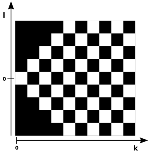
If the Radon transform is sampled over $2\pi$, the positions of the non-zero $b_{kl}$ form in the $(k,l)$-space a checkboarded wedge as shown in Fig. 1.
Consistency conditions have been extended to fan-beam [12] and cone-beam [13] geometry as well.

Figure 1: Checkboarded wedge pattern of the $b_{kl}$ coefficients in the $(k,l)$-space. The non-zero $b_{kl}$’s are placed in the white squares, the rest is zero.

3 Proposed method

The discrete version of $p(\theta,t)$ (also called sinogram) is indicated with $p[\theta_{h},t_{j}]$, where $\theta_{h}=h\pi/m\in[0,\pi)$ for $h=0,1,...,m-1$ and $t_{j}=-1+2j/(n-1)$ for $j=0,1,...,n-1$, considering $t_{j}\in[-1,1]$.
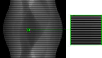
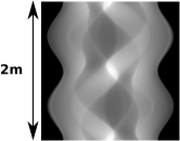
The proposed Helgason-Ludwig sinogram filter (HLSF) doubles the number of views of a sinogram $\in\mathbb{R}^{m\times n}$ by extrapolating $m$ missing projections at intermediate angles $\theta_{h+1/2}=(\theta_{h}+\theta_{h+1})/2$. The input sinogram is, first, interleaved with 0-valued projections, as shown in Fig. 2(a). In this way, it becomes an inconsistent dataset characterized by several non-zero $b_{kl}$’s at the locations indicated in (5) (Fig. 2(b)). By enforcing (5), consistency is recovered, the 0-valued lines are filled with extrapolated values and the resulting sinogram $\in\mathbb{R}^{2m\times n}$ can be reconstructed by means of an analytical method like FBP.
HLSF consists of the following four steps:

1. extension of the data to $[0,2\pi]$;

2. creation of an intermediate sinogram with $4m$ views; the $2m$ original projections are interleaved with $2m$ zero lines;

3. imposition of the HLCC on the intermediate inconsistent sinogram;

4. crop of the interval $[0,\pi)$ and reassignment of the original $m$ views.

(a)

(b)

Figure 2: Example of a sinogram interleaved with 0-valued lines (a) and the binarized real part of its Fourier-Chebyshev decomposition (b), showing that inconsistencies give rise to non-zero $b_{kl}$’s at the locations indicated in (5).

(a)

(b)

(c)

(d)

(e)

Figure 3: Succession of steps to compute the Fourier-Chebyshev decomposition of a sinogram. (a) Input sinogram of a Shepp-Logan phantom, $\theta\in[0,\pi)$. (b) Extended sinogram, $\theta\in[0,2\pi]$. (c) Interleaved sinogram. (d) Zoom-in of the region D in (c). (e) Sinogram with cosine-resampled projections.

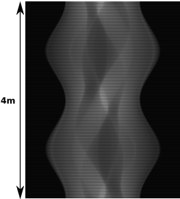
3.1 Step (1): extend sinogram to $[0,2\pi]$

First, the input sinogram, $p[\theta_{h},t_{j}]$, has to be extended to $[0,2\pi]$ in order to use (4):

$$\begin{split}&p^{(1)}[\theta_{h^{\prime}},t_{j}]=\begin{cases}p[\theta_{h},t_{j}]&\text{for}\hskip 2.84544pt\theta_{h^{\prime}}\in[0,\pi)\\[10.00002pt] p[\theta_{h},n-t_{j}]&\text{for}\hskip 2.84544pt\theta_{h^{\prime}}\in[\pi,2\pi)\end{cases}\hskip 2.84544pt\in\mathbb{R}^{2m\times n}\\[10.00002pt] &\hskip 28.45274pt\theta_{h^{\prime}}=\frac{\pi h^{\prime}}{m}\hskip 14.22636pth^{\prime}=0,1,...,2m-1\hskip 14.22636pt.\end{split}$$ (6)

Fig. 3(b) shows the result of extending the example sinogram in Fig. 3(a).

3.2 Step (2): interleaved sinogram

The interleaved sinogram $p^{(2)}[\theta_{h^{\prime\prime}},t_{j}]$ has $\theta_{h^{\prime\prime}}=h^{\prime\prime}\pi/2m$ for $h^{\prime\prime}=0,1,...,4m-1$ and corresponds to:

$$p^{(2)}[\theta_{h^{\prime\prime}},t_{j}]=\begin{cases}p^{(1)}[\theta_{h^{\prime}},t_{j}]&\text{for}\hskip 2.84544pth^{\prime\prime}=2h^{\prime}\\[10.00002pt] 0&\text{for}\hskip 2.84544pth^{\prime\prime}=2h^{\prime}+1\end{cases}\hskip 2.84544pt\in\mathbb{R}^{4m\times n}\hskip 8.5359pt.$$ (7)

An example of interleaved sinogram is shown in Fig. 3(c).

3.3 Step (3): imposing HLCC

By introducing the following quantities:

$$c_{k}(\theta)=\sum\limits_{l=-\infty}^{+\infty}b_{kl}\>e^{il\theta}\hskip 11.38092pt,$$ (8)

(4) can be rewritten as:

$$p(\theta,t)=\frac{1}{\pi}\sum\limits_{k=0}^{+\infty}c_{k}(\theta)\>(1-t^{2})^{1/2}\>U_{k}(t)\\$$ (9)

The $c_{k}(\theta)$’s are the Chebyshev coefficients of $[p(\theta,t)(1-t^{2})^{-1/2}]$; the $b_{kl}$’s are the Fourier series coefficients of the $c_{kl}$’s. The strategy consists in computing the $b_{kl}$ coefficients in two steps: first $p(\theta,t)$ is expanded onto the Chebyshev basis, then, the $b_{kl}$’s are retrieved from the $c_{k}(\theta)$’s.
The $c_{k}(\theta)$’s can be easily computed, by resampling the projections at points $t_{j}^{\prime}=\cos(\pi(j+1)/(n+1))$ [7, 14]. The cosine-resampling simplifies $U_{k}(t)$ into a sine function. Thus, the first term of (9) becomes:

$$p^{(2)}[\theta_{h^{\prime\prime}},t_{j}^{\prime}]=\sum\limits_{0}^{n-1}c_{k}[\theta_{h^{\prime\prime}}]\>\sin\left(\frac{\pi(j+1)(k+1)}{n+1}\right)\hskip 8.5359pt.$$ (10)

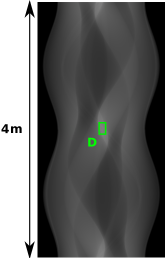
(10) shows that the $c_{k}[\theta_{h^{\prime\prime}}]$’s correspond to the type-1 discrete sine transform (DST-1) coefficients of the cosine-resampled projections (an example is provided by Fig. 3(e)).
After running the DST-1 along the channel direction of the sinogram, the $b_{kl}$’s are finally yielded by the FFT along the view direction:

$$b_{kl}=\frac{1}{4m}\>\text{DFT}\{c_{k}[\theta_{h^{\prime\prime}}]\}\hskip 8.5359pt.$$ (11)

Altogether, imposing the HLCC on $p^{(2)}[\theta_{h^{\prime\prime}},t_{j}]$ requires the cosine resampling, a DST-1 along the channel direction, a FFT along the view direction, setting to zero the $b_{kl}$’s according to (5) (Fig. 1) and reversing the process, i.e. an IFFT along the view direction, an IDSF-1 along the channel direction and resampling at positions $t_{j}$. The resulting sinogram is $p^{(3)}[\theta_{h^{\prime\prime}},t_{j}]\in\mathbb{R}^{4m\times n}$.

3.4 Step (4): crop in $[0,\pi)$ and reassign original data

The sinogram is, finally, cropped again in the interval $[0,\pi)$ and the original projections are reassigned.

4 Complexity and efficiency

The computational cost of the HLSF lies in the calls of the DST-1 along the channel direction and the FFT along the view direction. The computation of the DST can be factorized similarly to the FFT ($O(N\log_{2}N)$ complexity) plus few pre- and post-processing steps with $O(N)$ complexity [15]. For an input sinogram with $m$ views $\times$ $n$ pixels, this yields to approximately $8mn(\log_{2}n+\log_{2}4m)$ floating operations and a resulting $O(mn(\log_{2}n+\log_{2}4m))$ complexity.
To show that the proposed filter only slightly impacts the total reconstruction speed, a pure Matlab implementation of the HLSF has been compared to the well known Matlab function iradon. Results for sinograms of different sizes, collected in Tab. 1, prove that the HLSF requires smaller runtimes than a standard non-GPU implementation of FBP, especially for real datasets where $m,n>10^{3}$.

	HLSF	FBP
805 views $\times$ 512 pix.	0.22 s	0.30 s
1608 views $\times$ 1024 pix.	0.63 s	2.34 s
2500 views $\times$ 2048 pix.	1.65 s	14.50 s

Table 1: Comparison between the time elapsed to run the HLSF and the FBP reconstruction for sinograms of different sizes. HLSF is implemented in pure Matlab. FBP is performed by the Matlab function iradon.

5 Benchmark procedure

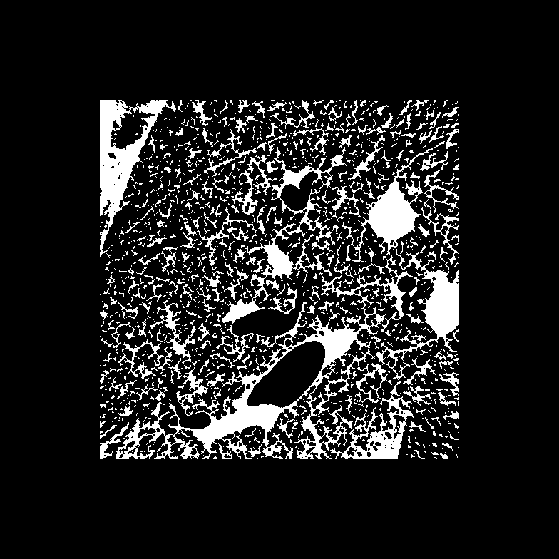
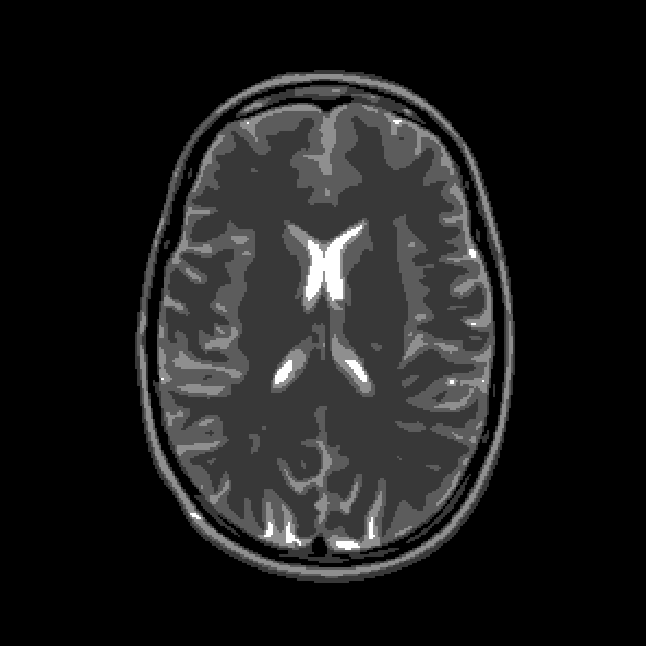
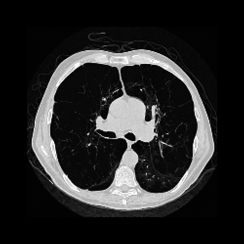
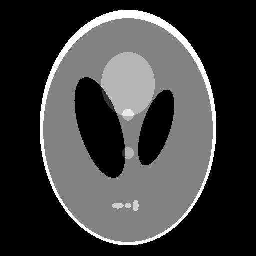
To assess the performance of the HLSF, four phantoms with structural patterns of different complexity have been considered (Fig. 4). PH-1 in Fig. 4(a) is the segmentation of a reconstructed slice of mouse lung tissue at micrometer scale. PH-2 in Fig. 4(b) is a multilevel segmentation of a MRI scan of a human brain. PH-3 in Fig. 4(c) is a multilevel segmentation of a CT slice of a human lung. PH-4 is the well-known Shepp-Logan phantom [16].
The simulated sinograms are computed by a standard space-based implementation of the Radon transform based on slant-stacking with linear interpolation [17].
Reconstructions are performed by means of FBP. The tradeoff between signal-to-noise ratio (SNR) and spatial resolution of FBP reconstructions is highly dependent on the choice of the filter function. For this reason, the dataset has been reconstructed with 3 different filters: a pure ramp or Ram-Lak filter and a ramp combined to a Hanning or Parzen [18] window to damp the high frequency components of the projections [11]. These filters are indicated in the following as Ram-Lak, Hanning and Parzen, respectively. The Ram-Lak filter provides the highest spatial resolution and the worst SNR, the opposite occurs for Parzen; Hanning is placed in the middle. Reconstructions labelled “CFBP” (Consistent FBP) were computed with FBP on a sinogram pre-filtered by HLSF with an upsampling factor of 2; reconstructions labelled “IFBP” (Interpolation FBP) were computed with FBP on a sinogram upsampled by a factor of 2 by means of 1D cubic spline interpolation along the view direction; otherwise they are simply labelled “FBP”.
The standard peak-signal-to-noise ratio (PSNR) [19], calculated within the reconstruction circle, is used to score each reconstruction with respect to the corresponding phantom.
The “sampling factor” (SF) is defined as the ratio between the number of projections of the considered sinogram and the number of projections of an optimally sampled sinogram. For parallel beam geometry, a sinogram is optimally sampled if $m\geq n\>\pi/2$, with $m$ the number of views and $n$ the number of detector pixels [11]. A sinogram with 100 views $\times$ 512 pixels, for example, considered well-sampled with $805\backsimeq 512\cdot\pi/2$ views, has SF = 0.12.

(a) PH-1

(b) PH-2

(c) PH-3

(d) PH-4

Figure 4: Set of simulated data used to benchmark the HLSF. PH-1 has 784 $\times$ 784 pixels; PH-2 has 592 $\times$ 592 pixels; PH-3 has 500 $\times$ 500 pixels; PH-4 has 512 $\times$ 512 pixels.

6 Experiments

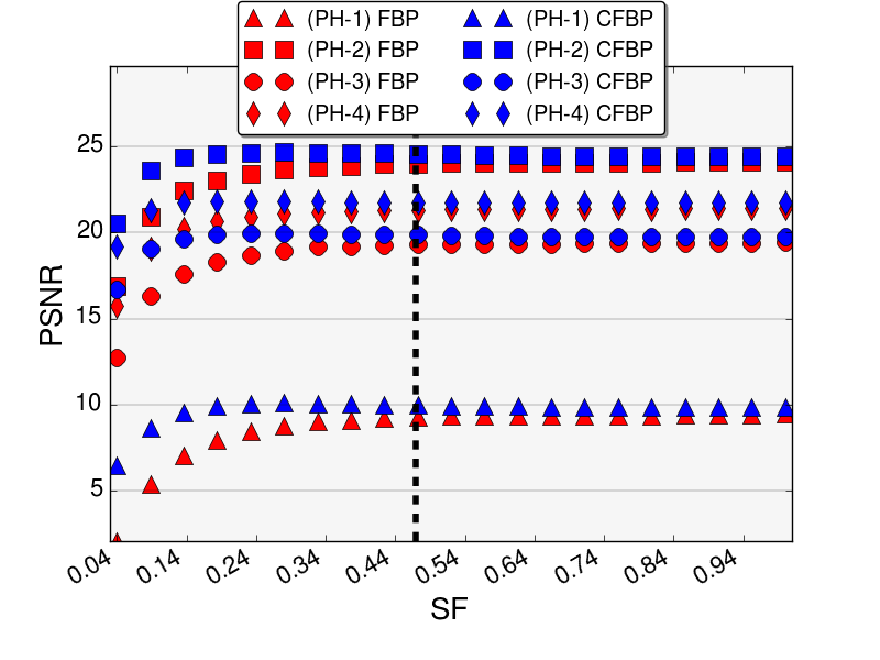
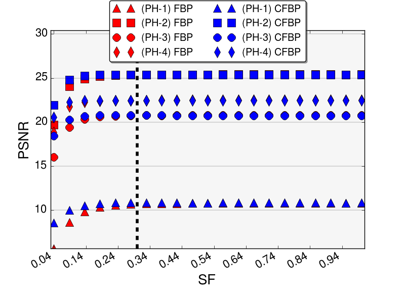
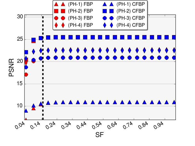
First, the performance of HLSF is tested for the noiseless case: noise-free sinograms with different SFs are reconstructed with FBP after pre-filtering with HLSF. The plots in Fig. 5 show that HLSF improves the reconstruction quality for small SF, while for higher SF the results for FBP and CFBP are comparable. The exact boundary between these 2 regimes depends on the filter choice. It is marked in Fig. 5 with a dashed black line and corresponds roughly to 0.47 for the Ram-Lak filter, 0.30 for Hanning and 0.15 for Parzen, regardless of the reconstructed object. The stronger the action of the filter, the smaller the SF interval where the HLSF increases the PSNR of the reconstruction.
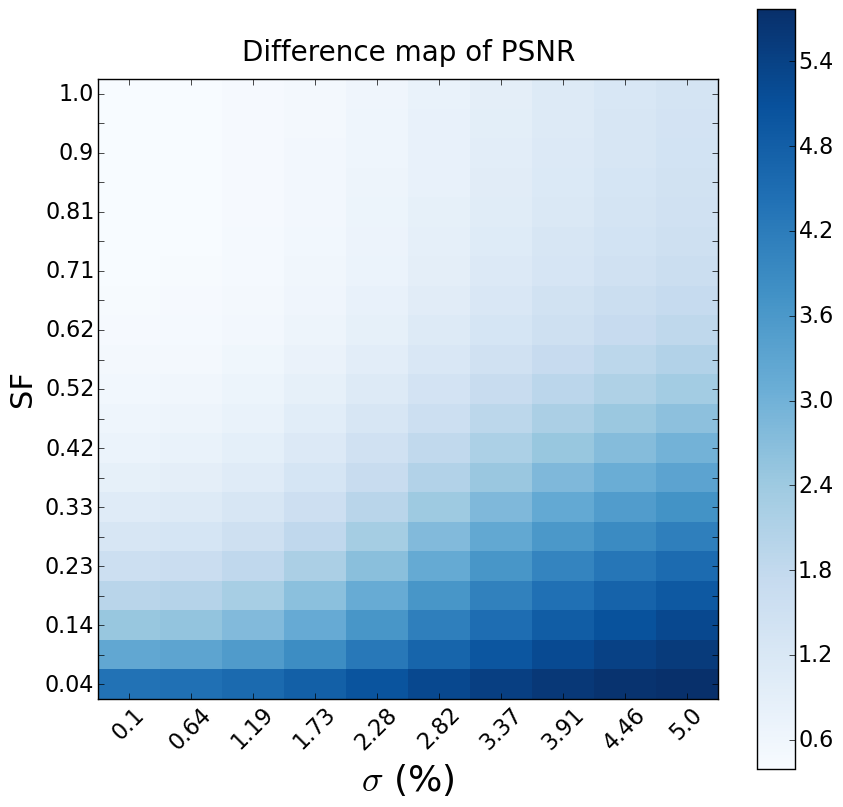
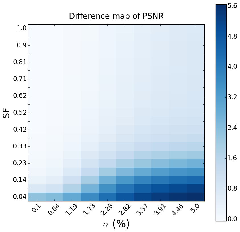
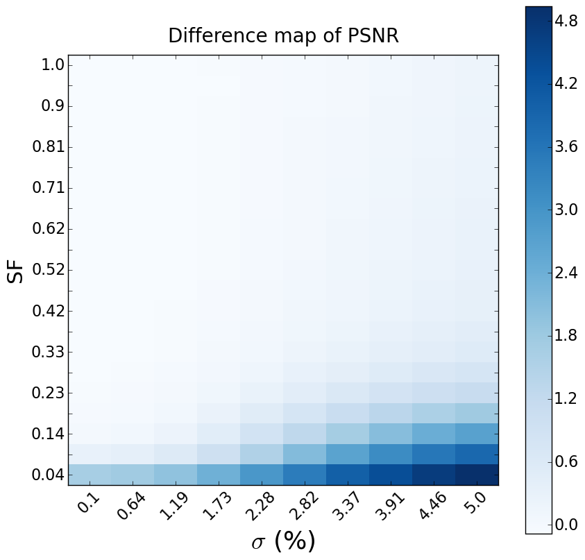
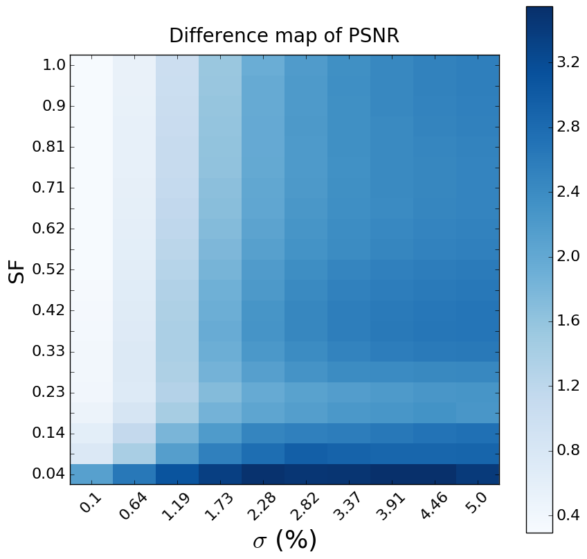
Subsequently, HLSF is also tested for noisy sinograms. The standard deviation of the added Poisson noise is expressed as percentage of the original sinogram mean value and is indicated with $\sigma$. Fig. 6 presents two-dimensional maps showing the difference between the PSNR score of CFBP and FBP reconstructions. Positive values indicate that CFBP outperforms FBP and viceversa. Each map corresponds to a specific choice of reconstruction filter and phantom.
The differential maps, shown in Fig. 6, are characterized by the same trend observed for the PSNR in Fig. 5: the stronger the action of the filter, the smaller the area, where HLSF provides a substantial improvement. However, CFBP reconstructions have always a higher PSNR compared to the FBP ones, since values on these maps are everywhere positive (Fig. 6).
Reconstructions with FBP and CFBP for each phantom are displayed in Fig. 7, 8, 9 and 10.

(a) Ram-Lak

(b) Hanning

(c) Parzen

Figure 5: PSNR scores as a function of the sampling factor, SF, of the FBP reconstructions performed with Ram-Lak, Hanning and Parzen filters. The red markers correspond to FBP reconstructions, the blue ones to CFBP reconstructions. The marker shape is related to the phantom used to create the simulated data.

(a) Ram-Lak (PH-1)

(b) Hanning (PH-2)

(c) Parzen (PH-3)

Figure 6: Maps of difference between PSNR scores of the CFBP and the FBP reconstructions as a function of the sampling factor, SF, and the variance, $\sigma$, of the additional Poisson noise. $\sigma$ is expressed as percentage of the original sinogram mean value. The caption of each map specifies what filter and phantom were used for the reconstructions.

(a) FBP

(b) CFBP

Figure 7: Reconstructions performed by FBP and CFBP with Ram-Lak filter of a PH-1 sinogram 168 views $\times$ 784 pixels (SF = 14%) + Poisson noise with $\sigma=2.2\%$ of the original sinogram mean value.

(a) FBP

(b) CFBP

Figure 8: Reconstructions performed by FBP and CFBP with Parzen filter of a PH-2 sinogram 82 views $\times$ 592 pixels (SF = 9%) + Poisson noise with $\sigma=2.8\%$ of the original sinogram mean value.

(a) FBP

(b) CFBP

Figure 9: Reconstructions performed by FBP and CFBP with Hanning filter of a PH-3 sinogram 108 views $\times$ 500 pixels (SF = 14%) + Poisson noise with $\sigma=2.2\%$ of the original sinogram mean value.

(a) FBP

(b) CFBP

Figure 10: Reconstructions performed by FBP and CFBP with Ram-Lak filter of a PH-4 sinogram 149 views $\times$ 512 pixels (SF = 18%) + Poisson noise with $\sigma=1.1\%$ of the original sinogram mean value.

(a) Ram-Lak

(b) Hanning

Figure 11: PSNR scores as a function of the sampling factor, SF, of the FBP reconstructions performed with Ram-Lak and Hanning filters. The red markers correspond to IFBP (cubic spline interpolation along the view direction + FBP) reconstructions, the blue ones to CFBP reconstructions. The marker shape is related to the phantom used to create the simulated data.

(a) Ram-Lak (PH-4)

(b) Hanning (PH-4)

(c) Parzen (PH-4)

Figure 12: Maps of difference between PSNR scores of the CFBP and the IFBP (cubic spline interpolation along the view direction + FBP) reconstructions as a function of the sampling factor, SF, and the variance, $\sigma$, of the additional Poisson noise. $\sigma$ is expressed as percentage of the original sinogram mean value. The caption of each map specifies what filter and phantom were used for the reconstructions.

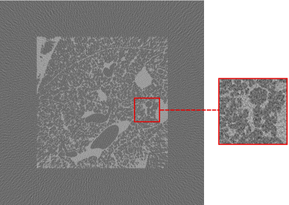
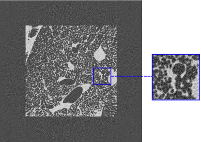
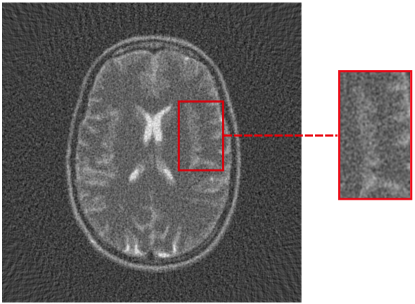
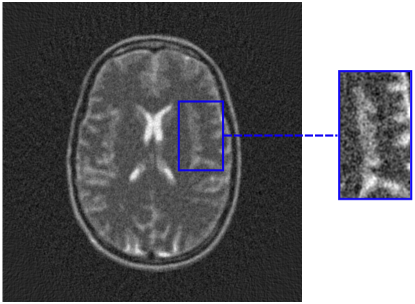
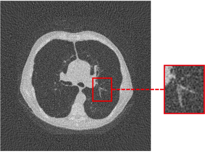
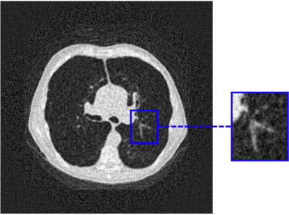
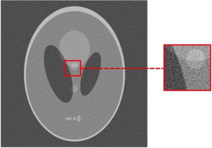
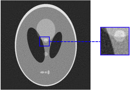
At visual inspection, the reconstructions with CFBP show better quality and details can be more easily identified.
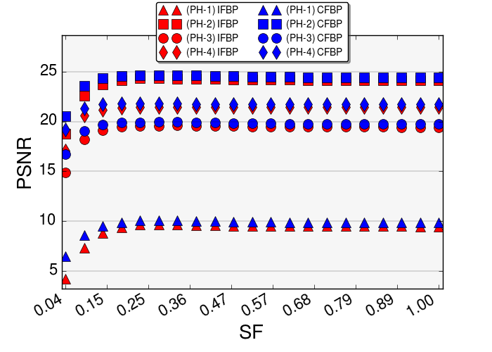
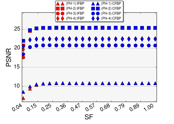
CFBP has also been compared to 1D cubic spline interpolation along the view direction (upsampling factor of 2) followed by FBP (IFBP). Simple 2D interpolation schemes used to double the number of views of a sinogram can yield visible artifacts on the FBP reconstruction and are, therefore, not considered here for comparison with HLSF. The algorithms are tested, first, on noiseless, then, on noisy datasets. Figure 11(a) shows that CFBP outperforms IFBP for any value of SF, when using the Ram-Lak filter, whereas differences vanish, when using the Hanning filter and SF$\,\gtrsim 0.30$, as illustrated by Fig. 11(b). Analogously to the results of Fig. 6, the stronger the action of the filter, the smaller the SF interval where CFBP can outperform IFBP for the reconstruction of noiseless undersampled datasets. 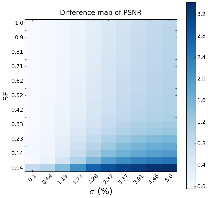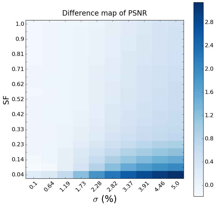The differential maps in Fig. 12 are everywhere positive (positive values correspond to $\text{PSNR}_{\text{CFBP}}(\sigma,\text{SF})>\text{PSNR}_{\text{IFBP}}(\sigma,\text{SF})$) and show that CFBP yields a better reconstruction quality than IFBP, especially for $\sigma>1.73$ and SF$\,<0.33$. Very similar results have also been obtained for PH-1, PH-2 and PH-3.
Other experiments (not shown here) have indicated that no additional improvement can be obtained from either applying HLSF multiple times sequentially or using HLSF to triple or quadruple at once the number of views.

7 Discussion and conclusion

This work presents a fast procedure to improve analytical tomographic reconstructions of undersampled datasets in parallel beam geometry. The proposed method is a filter working in the Radon domain and based on the Helgason-Ludwig consistency conditions. It doubles the number of views of a sinogram homogenously sampled in $[0,\pi)$, by extrapolating projections at intermediate angular positions.
This sinogram filter, abbreviated HLSF, is a non-iterative, parameterless procedure, that can be efficiently implemented with FFTs and only marginally impacts the total computational cost for analytical reconstructions.
Experiments, performed on data of different structural complexity, have shown that FBP reconstructions of sinograms pre-processed with the presented HLSF are charaterized by a higher PSNR compared to FBP reconstructions of standard sinograms. HLSF improves the reconstruction quality for both noiseless (generally, for SF ${\scriptstyle\lesssim}$ 0.31) and noisy undersampled (especially, for SF ${\scriptstyle\lesssim}$ 0.33 and $\sigma\>{\scriptstyle\gtrsim}\>1.73\%$) sinograms. Moreover, HLSF outperforms 1D cubic spline intepolation along the view direction: improvements in the reconstruction accuracy are substantial when dealing with noisy undersampled datasets (especially, for SF ${\scriptstyle\lesssim}$ 0.33 and $\sigma\>{\scriptstyle\gtrsim}\>1.73\%$).

References

- [1] Radon J. Über die Bestimmung von Funktionen durch ihre Integralwerte längs gewisser Mannigfaltigkeiten. Akad Wiss. 1917;69:262–277.
- [2] Ludwig D. The radon transform on euclidean space. Communications on Pure and Applied Mathematics. 2010 sep;19(1):49–81. Available from: http://dx.doi.org/10.1002/cpa.3160190105. doi:10.1002/cpa.3160190105.
- [3] Heyn E. Helgason, S., The Radon Transform. Progress in Mathematics 5. Boston-Basel-Stuttgart, Birkhäuser Verlag 1980. VII, 192 S., sFr. 15.–. ISBN 3-7643-3006-6. ZAMM - Zeitschrift für Angewandte Mathematik und Mechanik. 1981;61(8):411–411. Available from: http://dx.doi.org/10.1002/zamm.19810610835. doi:10.1002/zamm.19810610835.
- [4] Prince J, Willsky A. Constrained sinogram restoration for limited-angle tomography. Optical Engineering. 1990 5;29(5):535–544.
- [5] Kudo H, Saito T. Sinogram recovery with the method of convex projections for limited-data reconstruction in computed tomography. Journal of the Optical Society of America A. 1991 jul;8(7):1148. Available from: http://dx.doi.org/10.1364/JOSAA.8.001148. doi:10.1364/josaa.8.001148.
- [6] Gompel GV, Defrise M, Dyck DV. Elliptical extrapolation of truncated 2D CT projections using Helgason-Ludwig consistency conditions. In: Flynn MJ, Hsieh J, editors. Medical Imaging 2006: Physics of Medical Imaging. SPIE-Intl Soc Optical Eng; 2006. Available from: http://dx.doi.org/10.1117/12.653293. doi:10.1117/12.653293.
- [7] Xu J, Taguchi K, Tsui BMW. Statistical Projection Completion in X-ray CT Using Consistency Conditions. IEEE Transactions on Medical Imaging. 2010 aug;29(8):1528–1540. Available from: http://dx.doi.org/10.1109/TMI.2010.2048335. doi:10.1109/tmi.2010.2048335.
- [8] Yu H, Wang G. Data Consistency Based Rigid Motion Artifact Reduction in Fan-Beam CT. IEEE Transactions on Medical Imaging. 2007 feb;26(2):249–260. Available from: http://dx.doi.org/10.1109/TMI.2006.889717. doi:10.1109/tmi.2006.889717.
- [9] Alessio AM, Kinahan PE, Champley KM, Caldwell JH. Attenuation-emission alignment in cardiac PET/CT based on consistency conditions. Med Phys. 2010;37(3):1191. Available from: http://dx.doi.org/10.1118/1.3315368. doi:10.1118/1.3315368.
- [10] Herman GT. Image Reconstruction from Projections: Implementation and Applications (Topics in Applied Physics). Springer; 1979.
- [11] Kak AC, Slaney M. Principles of Computerized Tomographic Imaging (Classics in Applied Mathematics). Society for Industrial and Applied Mathematics; 2001.
- [12] Chen GH, Leng S. A new data consistency condition for fan-beam projection data. Med Phys. 2005;32(4):961. Available from: http://dx.doi.org/10.1118/1.1861395. doi:10.1118/1.1861395.
- [13] Clackdoyle R, Desbat L. Full data consistency conditions for cone-beam projections with sources on a plane. Physics in Medicine and Biology. 2013 nov;58(23):8437–8456. Available from: http://dx.doi.org/10.1088/0031-9155/58/23/8437. doi:10.1088/0031-9155/58/23/8437.
- [14] Bortfeld T, Oelfke U. Fast and exact 2D image reconstruction by means of Chebyshev decomposition and backprojection. Physics in Medicine and Biology. 1999;44(4):1105. Available from: http://stacks.iop.org/0031-9155/44/i=4/a=020.
- [15] Poularikas AD. The Transforms and Applications Handbook, Second Edition (Electrical Engineering Handbook). CRC Press; 2000.
- [16] Shepp LA, Logan BF. The Fourier reconstruction of a head section. IEEE Trans Nucl Sci. 1974 jun;21(3):21–43. Available from: http://dx.doi.org/10.1109/TNS.1974.6499235. doi:10.1109/tns.1974.6499235.
- [17] Toft P. The Radon Transform. Theory and Implementation. Department of Mathematical Modelling, Section for Digital Signal Processing, Technical University of Denmark; 1996. Available from: https://books.google.ch/books?id=s7EPYAAACAAJ.
- [18] Lyra M, Ploussi A. Filtering in SPECT Image Reconstruction. International Journal of Biomedical Imaging. 2011;2011:1–14. Available from: http://dx.doi.org/10.1155/2011/693795. doi:10.1155/2011/693795.
- [19] Huynh-Thu Q, Ghanbari M. Scope of validity of PSNR in image/video quality assessment. Electron Lett. 2008;44(13):800. Available from: http://dx.doi.org/10.1049/el:20080522. doi:10.1049/el:20080522.
- [20] Schomberg H, Timmer J. The gridding method for image reconstruction by Fourier transformation. IEEE Transactions on Medical Imaging. 1995;14(3):596–607. Available from: http://dx.doi.org/10.1109/42.414625. doi:10.1109/42.414625.