Image Denoising via Multi-scale Nonlinear Diffusion Models

Abstract

Image denoising is a fundamental operation in image processing and holds considerable practical importance for various real-world applications. Arguably several thousands of papers are dedicated to image denoising. In the past decade, sate-of-the-art denoising algorithm have been clearly dominated by non-local patch-based methods, which explicitly exploit patch self-similarity within image. However, in recent two years, discriminatively trained local approaches have started to outperform previous non-local models and have been attracting increasing attentions due to the additional advantage of computational efficiency. Successful approaches include cascade of shrinkage fields (CSF) and trainable nonlinear reaction diffusion (TNRD). These two methods are built on filter response of linear filters of small size using feed forward architectures. Due to the locality inherent in local approaches, the CSF and TNRD model become less effective when noise level is high and consequently introduces some noise artifacts. In order to overcome this problem, in this paper we introduce a multi-scale strategy. To be specific, we build on our newly-developed TNRD model, adopting the multi-scale pyramid image representation to devise a multi-scale nonlinear diffusion process. As expected, all the parameters in the proposed multi-scale diffusion model, including the filters and the influence functions across scales, are learned from training data through a loss based approach. Numerical results on Gaussian and Poisson denoising substantiate that the exploited multi-scale strategy can successfully boost the performance of the original TNRD model with single scale. As a consequence, the resulting multi-scale diffusion models can significantly suppress the typical incorrect features for those noisy images with heavy noise. It turns out that multi-scale TNRD variants achieve better performance than state-of-the-art denoising methods.

1 Introduction

Image denosing is a widely studied problem with immediate practical applications in image processing and computer vision, serving as a preprocessing step. During the past decades, many remarkable denoising methods have been proposed to improve the performance of single-image based denoising. Up to now, image denoising still remains a vibrant research field [6]. Roughly speaking, image denoising techniques can be classified into two categories: (1) nonlocal methods, which exploit nonlocal similarity information within long range distance, such as [11, 14], or global information in the whole image [37] or even similar patches from an external dataset [41]; and (2) local methods, which solely depend on information in a local neighborhood, such as [33, 12].

For the present, most existing state-of-the-art image denoising algorithms are based on exploiting nonlocal similarity between a relatively modest number of patches, for instance, Gaussian denoising [24, 14, 11], multiplicative noise reduction [9], [30] and Poisson noise suppression [35], [13]. The basic idea of the nonlocal approaches is to estimate the target pixel based on a carefully selected set of pixels: not just those closest to the target but also those distant pixels that are more likely to have the same underlying signal. Usually, the goal of nonlocal techniques mainly concentrate on achieving utmost image restoration quality, but with little consideration on the computational efficiency. As a consequence, predominant state-of-the-art image denoising approaches are without a doubt non-local models.

In contrast to nonlocal denoising approaches, local methods merely investigate the local information from the surrounding pixels to denoise the central pixel. Since the well-known P-M model [31] and ROF model [34], many attempts have been made to develop effective local models, such as Product of Experts (PoT) [40], Fields of Experts (FoE) framework [33] and K-SVD [12]. Due to the inherent drawback of locality, one would not expect a local model can compete with those good-performing nonlocal approaches. However, in recent years a few local models, e.g., [43, 3, 7], obtained from elaborate learning are able to produce comparable results to state-of-the-arts, such as BM3D [11]. Especially, two newly-developed local models - the CSF [36] and TNRD model [8], which are also discriminatively trained, successfully achieve superior denoising performance to previous state-of-the-arts. Therefore, discriminative model learning for image denoising has been attracting more and more attentions as it additionally bears a significant merit of computational efficiency.

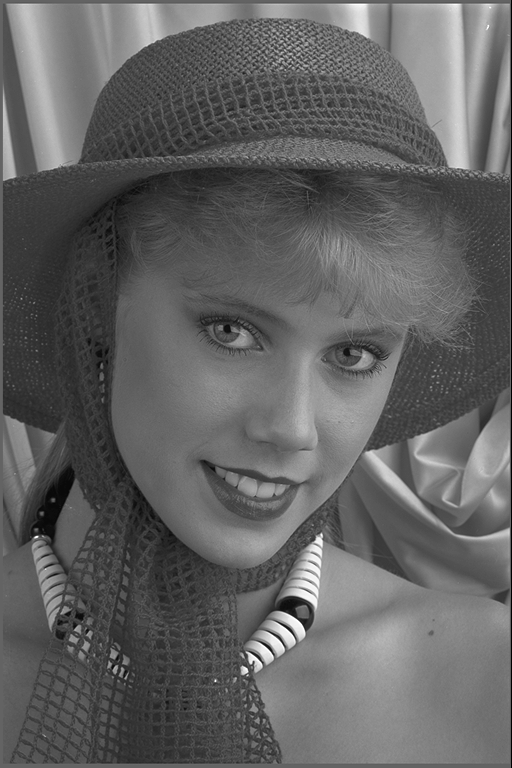
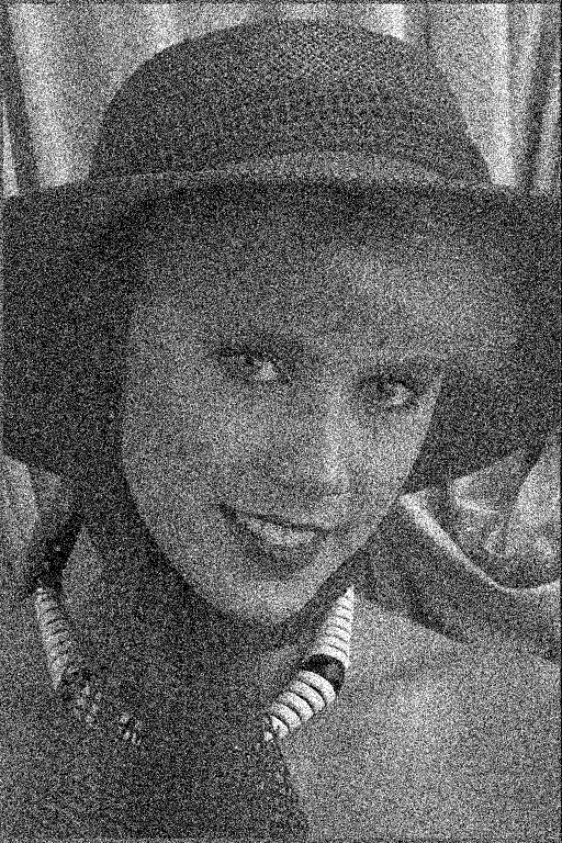
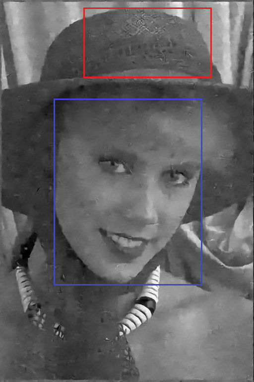
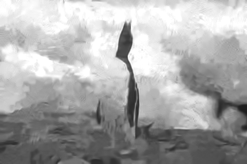
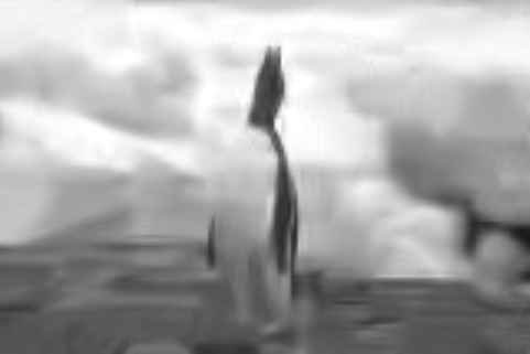
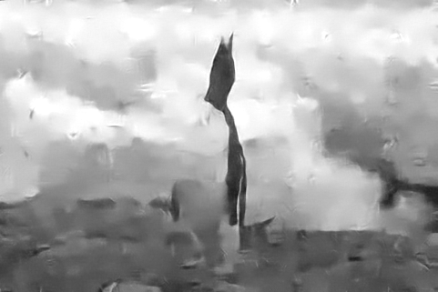
As aforementioned, local models infer the underlying structure solely from the local neighborhoods. Despite the general effectiveness of the CSF and TNRD model, they can not avoid this inherent drawback. As a consequence, when the noise level is relatively high, some incorrect image features, which are not in the clean image, appear in the denoised results. In this case, local image structures are heavily distorted by noise (as shown in Fig. 1)(c), and therefore it becomes very challenging to estimate these structures. Under this circumstance, a larger region containing larger-scale information would benefit for effective denoising.

A deeper inspection of the CSF and TNRD model reveals that it is the small size of involved filters that causes these approaches to ignore larger-scale information. So we hypothesize that these two denoising algorithms can be improved by employing a multi-scale strategy.

(a) Clean Image

(b) Noisy image. $\sigma=50$

(c) $\mathrm{TNRD}_{5\times 5}^{5}$ (28.58/0.718)

(d) $\mathrm{MSND}_{5\times 5}^{5}$ (28.95/0.730)

Figure 1: Gaussian noise denoising results comparison. The results are reported by PSNR/SSIM index. Better result is marked. We can see that MSND model achieves apparent improvements in the highlighted regions, such as face and hat.

1.1 Multi-scale strategy

Multi-scale analysis, which becomes a standard tool in image analysis, has been widely exploited for diverse image processing problems, such as image segmentation [23], hyper-spectral image classification [16], single image defogging [38], single image dehazing [1] and the image denoising task investigated in this paper [18, 42, 4]. Generally speaking, multi-scale analysis can represent distinct but complementary information that exists at coarse-to-fine resolution levels. Therefore, such representations reveal more structural information about signals and offer a number of advantages over fixed-scale methods.

In the context of Wavelet transform based image processing, multi-scale analysis can be naturally incorporated as the Wavelet transforms usually decompose an image in a multi-scale manner. A few Wavelet based image denoising algorithms can deliver appealing performance [5, 32] via the well-known Wavelet shrinkage operation.

In the case of image denoising, multi-scale analysis is more commonly understood as image pyramid, i.e., down-sampling the input image to build the noisy pyramid. As pointed out in [18, 4] that multi-scale analysis would be generally beneficial to image denoising, as it promises at least two improvements

• Down-sampling has a denoising effect. For the particular case of Gaussian white noise, consider down-sampling a noisy image by a factor of two in the way that distinct blocks of four pixels are averaged to form a single pixel in the low-resolution image, the standard deviation of the noise will be divided by two compared to the noise contained in original noisy image. Therefore, down-sampling can cause the uncorrelated values of the noise to become smaller and consequently make image structures more visible, which can be clearly observed by visual comparison on (c) and (d) in Fig. 1.

• Down-sampling the image before denoising amounts to enlarge the size of the neighborhood on which the denoising is performed, thus permitting to exploit larger-scale information. This will be particularly helpful for those local models considered in this paper.

Due to the above-mentioned potential benefits from the multi-scale strategy, it has been employed by many image denoising algorithms. Zontak et al.proposed using the patch recurrence across scales to separate signal from noise [42]. In [18], a multi-scale scheme was exploited for blind denoising, and a multi-scale meta-procedure was considered to improve the performance of a few denoising algorithms [4]. In [22] and [20], a multi-scale representation was constructed to perform progressive image denoising and Poisson denoising, respectively.

1.2 Motivation and contributions

The above-mentioned works substantiate the usefulness of the multi-scale structure. Therefore, it is intriguing to incorporate the multi-scale strategy in the newly developed TNRD framework [8] to investigate whether it can also boost the performance of the TNRD model with single scale. In this paper, we only concentrate on the TNRD framework, as it exhibits a remarkable advantage of high efficiency over existing denoising algorithms, besides its compelling denoising performance.

In this work, we incorporate the multi-scale strategy into the TNRD framework, resulting in a novel image denoising approach named as Multi-scale Nonlinear Diffusion Model (MSND). Thus, the image diffusion process happens in a few scales instead of in a single scale, and the resulting images are combined into a single denoised image in the finest scale via up-sampling. As usual in discriminative model learning for image denoising, all the parameters in the proposed multi-scale model, including the filters and the influence functions, are supervised learned end-to-end with training samples.

In order to verify the validity of the multi-scale strategy in the TNRD framework for image denoising, we investigate denoising problems for two typical types of noise: Gaussian noise and Poisson noise. Numerical experiments on Gaussian and Poisson denoising demonstrate that the resulting multi-scale TNRD models can considerably improve the performance of the single scale counterparts, especially when the noise level is high, therein the multi-scale TNRD models can significantly suppress the typical incorrect features appearing in the original TNRD models, as shown within the blue rectangle in Fig. 1(c) and (d). It turns out that the resulting MSND models yield better performance than state-of-the-art denoising approaches.

To summarize, the main contributions of this paper are three folds.

• We extend the TNRD framework with a multi-scale strategy, which can significantly enlarge the size of local receptive field exploited for diffusion;

• We demonstrate the versatility of the TNRD framework and its multi-scale variant through an additional image denoising problem at the presence of Poisson noise;

• Extensive experimental results substantiate the usefulness of the multi-scale procedure, especially in the case of heavy noise. It turns out that the multi-scale nonlinear diffusion models can surpass state-of-the-art denoising algorithms.

The remainder of the paper is organized as follows. Section II presents a general review of the trainable nonlinear reaction diffusion process. In the subsequent section III, we propose the Image Denoising approach via Multi-scale Nonlinear Diffusion, and take it for Gaussian noise removing and Poisson noise removing. Subsequently, Section IV describes comprehensive experiment results for the proposed model. The concluding remarks are drawn in the final Section V.

2 Preliminaries

To make the paper self-contained, in this section we provide a brief review of the trainable nonlinear diffusion process proposed in [8].

2.1 Highly parametrized nonlinear diffusion model

In our recent work [8], a simple but effective framework for image restoration called TNRD was proposed based on the concept of nonlinear reaction diffusion. The TNRD framework is modeled by highly parametrized linear filters as well as highly parametrized influence functions. In contrast to those conventional nonlinear diffusion models which usually make use of handcrafted parameters, all the parameters in the TNRD model, including the filters and the influence functions, are learned from training data through a loss based approach.

The general framework of the TNRD model is formulated as the following time-dynamic nonlinear reaction-diffusion process with $T$ steps

$$\small\begin{cases}u_{0}=I_{0}\\ u_{t}=\underbrace{\text{Prox}_{\mathcal{G}^{t}}}_{\text{reaction force}}\left(u_{t-1}-\left(\underbrace{\sum\limits_{i=1}^{N_{k}}(K_{i}^{t})^{\top}\phi_{i}^{t}(K_{i}^{t}u_{t-1})}_{\text{diffusion force}}+\underbrace{\psi^{t}(u_{t-1},f)}_{\text{reaction force}}\right)\right)\,,\\ t=1\cdots T\,,\end{cases}$$ (2.1)

where image $u$ is represented as a column vector, i.e., $u\in\mathbb{R}^{N}$, $I_{0}$ is the initial status of the diffusion process and $T$ denotes the diffusion stages. $K_{i}\in\mathbb{R}^{N\times N}$ is a highly sparse matrix, implemented as 2D convolution of the image $u$ with the linear filter $k_{i}$, i.e., $K_{i}u\Leftrightarrow k_{i}*u$, $K_{i}$ is a set of linear filters and $N_{k}$ is the number of filters. In this formulation, function $\phi_{i}$ is known as influence function and is applied point-wise to the filter response, i.e., $\phi(K_{i}u)=\left(\phi(K_{i}u)_{1},\cdots,\phi(K_{i}u)_{N}\right)^{\top}\in\mathbb{R}^{N}$.

Both the proximal mapping operation $\text{Prox}_{\mathcal{G}}(\hat{u})$ and $\psi(u_{t},f)$ are related to the reaction force. The proposed TNRD can be applied to various image restoration problems by exploiting task-specific function $\mathcal{G}(u,f)$ and $\psi(u,f)$. Usually, the reaction term $\psi(u)$ is designated as the derivative of a certain smooth date term $\mathcal{D}(u,f)$, i.e., $\psi(u)=\nabla_{u}\mathcal{D}(u)$. The term $\mathcal{G}(u,f)$ is used to handle those problems with a non-smooth date term, e.g., JPEG deblocking in [8] or a data term for which a gradient descent step is not appropriate, e.g., Poisson denoising investigated in this paper. Note that the proximal mapping operation [28] related to the function $\mathcal{G}^{t}$ is given as

$$\text{Prox}_{\mathcal{G}^{t}}(\hat{u})=\min\limits_{u}\frac{\|u-\hat{u}\|_{2}^{2}}{2}+\mathcal{G}^{t}(u,f)\,.$$

The diffusion term involves trainable linear filters and influence functions (nonlinearities) and these parameters vary in each iteration, i.e., time varying linear filters and nonlinearities.

As shown in [8], the proposed model (2.1) can be interpreted as performing one gradient descent step at $u^{t}$ with respect to a dynamic energy functional given by

$$E^{t}(u,f)=\sum\nolimits_{i=1}^{N_{k}}\sum\limits_{p=1}^{N}\rho_{i}^{t}((k_{i}^{t}*u)_{p})+\mathcal{D}^{t}(u,f)+\mathcal{G}^{t}(u,f)\,,$$ (2.2)

where the functions $\left\{\rho_{i}^{t}\right\}_{t=1}^{t=T}$ are the so-called penalty functions. Note that $\rho^{\prime}(z)=\phi(z)$ and the parameters {$k_{i}^{t},\rho_{i}^{t}$} vary across the stages i.e., changes at each iteration.

The TNRD model also bears an interesting link to convolutional networks (CNs) applied to image restoration problems in [15]. For example, from the architecture of our proposed diffusion model for Gaussian denoising, shown in Figure 2, one can see that each iteration (stage) of our proposed diffusion process involves convolution operations with a set of linear filters, and thus it can be treated as a convolutional network. The most noticeable aspect in the proposed convolutional network is that the nonlinearities (i.e., influence functions in the context of nonlinear diffusion) are trainable, instead of a fixed activation function, e.g., the ReLU function [27] or sigmoid functions [15], in conventional CNs.

The TNRD framework is applicable to different image restoration problems by incorporating specific reaction force, such as Gaussian denoising and Poisson denoising investigated in this paper. For Gaussian denoising, it is realized by setting $\mathcal{G}^{t}=0$, while $\mathcal{D}^{t}(u,f)=\frac{\lambda^{t}}{2}\|u-f\|_{2}^{2}$ and $\psi^{t}(u)=\lambda^{t}(u-f)$, where $\lambda^{t}$ is related to the strength of the reaction term, $f$ denote the input degraded image.

In the case of Poisson denoising, taking into account the peculiar features of Poisson noise, the relevant data term is given by the so-called Csiszár I-divergence model [10, 17, 13], defined as

$$\langle u-f\mathrm{log}u,1\rangle,$$ (2.3)

where $\langle,\rangle$ denotes the standard inner product. Then, in the proposed model, we set $\mathcal{D}^{t}=0$, while $\mathcal{G}^{t}(u,f)={\lambda^{t}}\langle u-f\mathrm{log}u,1\rangle$. More details can be found in Sec. 3.3.

2.2 Overall training scheme

The TNRD model in (2.1) is trained in a supervised manner, namely, the input/output pairs for certain image processing task are firstly prepared, and then we exploit a loss minimization scheme to optimizet the model parameters $\Theta^{t}$ for each stage $t$ of the diffusion process. The training dataset consists of $S$ training samples $\{u_{gt}^{s},f^{s}\}_{s=1}^{S}$, where $u_{gt}^{s}$ is a ground truth image and $f^{s}$ is the corresponding degraded input. The model parameters in stage $t$ required to be trained include 1) the reaction force weight $\lambda$, (2) linear filters and (3) influence functions. All parameters are grouped as $\Theta^{t}$, i.e., $\Theta^{t}=\{\lambda^{t},\phi_{i}^{t},k_{i}^{t}\}$. Then, the optimization problem for the training task is formulated as follows

$$\small\begin{cases}\min\limits_{\Theta}\mathcal{L}(\Theta)=\sum\limits_{s=1}^{S}\ell(u_{T}^{s},u_{gt}^{s})=\sum\limits_{s=1}^{S}\frac{1}{2}\|u_{T}^{s}-u_{gt}^{s}\|^{2}_{2}\\ \text{s.t.}\begin{cases}u_{0}^{s}=I_{0}^{s}\\ u_{t}^{s}=\text{Prox}_{\mathcal{G}^{t}}\left(u_{t-1}^{s}-\left({\sum\limits_{i=1}^{N_{k}}(K_{i}^{t})^{\top}\phi_{i}^{t}(K_{i}^{t}u_{t-1}^{s})}+\psi^{t}(u_{t-1}^{s},f^{s})\right)\right),\\ t=1\cdots T\,,\end{cases}\end{cases}$$ (2.4)

where $\Theta=\{\Theta^{t}\}_{t=1}^{t=T}$. The training problem in (2.4) can be solved via gradient based algorithms, e.g., the L-BFGS algorithm [21], where the gradients associated with $\Theta_{t}$ are computed using the standard back-propagation technique [19].

There are two training strategies to learn the diffusion processes: 1) the greedy training strategy to learn the diffusion process stage-by-stage; and 2) the joint training strategy to train a diffusion process by simultaneously tuning the parameters in all stages. Generally speaking, the joint training strategy performs better [8], and the greedy training strategy is often used to provide a good initialization for the joint training. Concerning the joint training scheme, the gradients $\frac{\partial\ell(u_{T},u_{gt})}{\partial\Theta_{t}}$ are computed as follows,

$$\frac{\partial\ell(u_{T},u_{gt})}{\partial\Theta_{t}}=\frac{\partial u_{t}}{\partial\Theta_{t}}\cdot\frac{\partial u_{t+1}}{\partial u_{t}}\cdots\frac{\partial\ell(u_{T},u_{gt})}{\partial u_{T}}\,,$$ (2.5)

which is known as back-propagation. For different image restoration problems, we mainly need to recompute the two components $\frac{\partial u_{t}}{\partial\Theta_{t}}$ and $\frac{\partial u_{t+1}}{\partial u_{t}}$, the main part of which are similar to the derivations in [8].

3 The Proposed Multi-scale Nonlinear Diffusion Model

Figure 2: The architecture of the proposed multi-scale diffusion model for Gaussian denoising. It is represented as a multi-layer feed-forward network. Note that the additional convolution step with the rotated kernels $\bar{k}_{i}$ (cf. Equ. 3.3) does not appear in conventional feed-forward CNs.

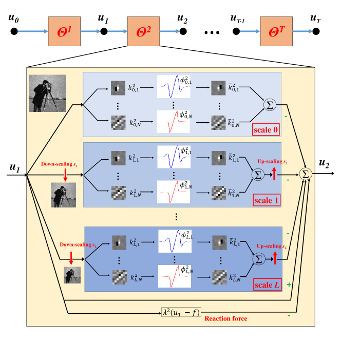
When the noise level is relatively high, the TNRD model will introduce some artifacts in the denoised images. The resulting artifacts are more apparent in the homogeneous regions of the image, typical of commonplace images such as scenery and landscapes. As aforementioned, in order to alleviate this phenomenon, in this paper, we introduce a multi-scale version of the TNRD algorithm, namely, we adopt the multi-scale pyramid image representation to devise a multi-scale nonlinear diffusion process.

3.1 General formulation of the proposed multi-scale diffusion model

The basic idea is to extend the diffusion term in the TNRD model (2.1) to a multi-scale version. As a result, the new diffusion term in the stage $t$ is given as

$$\sum\limits_{l=0}^{L}\sum\limits_{i=1}^{N_{k}}A_{l}^{\top}(K_{l,i}^{t})^{\top}\phi_{l,i}^{t}(K_{l,i}^{t}A_{l}u_{t-1})\,,$$ (3.1)

where $L$ is the number of total scales exploited in the proposed model, and the additional linear operator $A_{l}$ is related to down-sampling the original image $u$ to different sizes, i.e., different scales. For example, $A_{0}$ is the identity matrix without any change to the original image and $A_{l}$ corresponds to down-sampling the original image with a factor $s^{l-1}$, where $s$ is the scale factor for the adjacent image in the scale space. In this paper, the down-sampling operator $A_{l}$ is constructed in the following form, taking for instance the scale factor of 2

$$\begin{array}[]{c}A_{l}\left[\begin{array}[]{cccc}u_{11}&u_{12}&u_{13}&u_{14}\\ u_{21}&u_{22}&u_{23}&u_{24}\\ u_{31}&u_{32}&u_{33}&u_{34}\\ u_{41}&u_{42}&u_{43}&u_{44}\end{array}\right]=\frac{1}{4}\left[\begin{array}[]{cc}{u_{11}}+{u_{12}}+{u_{21}}+{u_{22}}&{u_{13}}+{u_{14}}+{u_{23}}+{u_{24}}\\ {u_{31}}+{u_{32}}+{u_{41}}+{u_{42}}&{u_{33}}+{u_{34}}+{u_{43}}+{u_{44}}\end{array}\right].\end{array}$$

For other cases, the formulation of $A_{l}$ can be similarly derived. Note that in (3.1) the operator $A_{l}^{\top}$ refers to the corresponding up-sampling operator to enlarge the low resolution image to the original size.

In summary, the proposed multi-scale framework is formulated as the time-dynamic nonlinear reaction-diffusion process with $T$ steps shown in (3.2). In the training phase, this new diffusion process is plugged into the training framework (2.4) to replace the single scale based diffusion procedure. The parameters to be trained in stage $t$ include $\{\{\phi_{l,i}^{t},k_{l,i}^{t}\}_{l=0}^{L}\}_{i=1}^{N_{k}}$ and the parameter $\lambda^{t}$ associated with the reaction force $\psi^{t}(u_{t-1},f)$ or $\mathcal{G}(u,f)$, which are grouped into to $\Theta^{t}=\left\{\{\{\phi_{l,i}^{t},k_{l,i}^{t}\}_{l=0}^{L}\}_{i=1}^{N_{k}},\lambda^{t}\right\}$. Remember that these parameters are optimized with a gradient-based algorithm, and therefore, we have to compute the gradients of the loss function with respect to $\Theta^{t}$. According to the basic chain rule (2.5), we mainly need to compute the derivations of $\frac{\partial u_{t}}{\partial\Theta^{t}}$ and $\frac{\partial u_{t+1}}{\partial u_{t}}$, as the gradient $\frac{\partial\ell(u_{T},u_{gt})}{\partial u_{T}}$ is simply given as $\frac{\partial\ell(u_{T},u_{gt})}{\partial u_{T}}=u_{T}-u_{gt}\,.$

$$\begin{cases}u_{t}=\underbrace{\text{Prox}_{\mathcal{G}^{t}}}_{\text{reaction force}}\left(u_{t-1}-\left(\underbrace{\sum\limits_{l=0}^{L}\sum\limits_{i=1}^{N_{k}}A_{l}^{\top}(K_{l,i}^{t})^{\top}\phi_{l,i}^{t}(K_{l,i}^{t}A_{l}u_{t-1})}_{\text{diffusion force}}+\underbrace{\psi^{t}(u_{t-1},f)}_{\text{reaction force}}\right)\right)\,,\\ \text{with}\quad u_{0}=I_{0},\quad t=1\cdots T\,.\end{cases}$$ (3.2)

In the following subsections, we present the main results of the gradients for two exploited denoising problems, and the detailed derivation steps are referred to the notes for diffusion network [8].

3.2 Gradients for the case of Gaussian denoising

For the Gaussian denoising problem, the multi-scale diffusion process is given as

$$\small u_{t}=u_{t-1}-\left(\sum\limits_{l=0}^{L}\sum\limits_{i=1}^{N_{k}}A_{l}^{\top}\left(\bar{k}_{l,i}^{t}*\phi_{l,i}^{t}(k_{l,i}^{t}*A_{l}u_{t-1})\right)+\lambda^{t}(u_{t-1}-f)\right)\,,$$ (3.3)

where the convolution kernel $\bar{k}_{i}$ (obtained by rotating the kernel $k_{i}$ 180 degrees) is explicitly used to replace $K_{i}^{\top}$ for the sake of model simplicity. In this formulation, image $u$ is understood as a 2D matrix. The corresponding diffusion procedure is illustrated in Figure 2. Note that notation $A_{l}$ in this formulation is in a little misusage. We should bear in mind that when operating with $A_{l}$ and $A_{l}^{\top}$, the image $u$ is understood as a column vector.

In the following derivations, as we frequently encounter the convolution operation $k*u$ (image $u\in\mathbb{R}^{m\times n}$, $k\in\mathbb{R}^{r\times r}$), it is helpful to exploit the equivalence for convolution: $k*u\Longleftrightarrow Ku\Longleftrightarrow Uk\,.$ That is to say, $k*u$ is equivalent to the matrix-vector product formulation $Ku$, where $K\in\mathbb{R}^{N\times N}$ is a highly sparse matrix and $u$ is a column vector $u\in\mathbb{R}^{N}$ with $N=m\times n$. It can also be interpreted with $Uk$, where matrix $U\in\mathbb{R}^{N\times R}$ is constructed from image $u$ and $k$ is a column vector $k\in\mathbb{R}^{R}$ with $R=r\times r$. The latter form is particularly helpful for the computation of the gradients of the loss function with respect to the kernel $k$, as $U^{\top}v$ ($v\in\mathbb{R}^{N}$ is a column vector) can be explicitly interpreted as a convolution operation, which is widely used in classic convolutional neural networks [2]. Furthermore, we consider the denominator layout notation for matrix calculus required for the computation of derivations, where the basic chain rule is given as the following order

$$\frac{\partial z}{\partial x}=\frac{\partial y}{\partial x}\cdot\frac{\partial z}{\partial y}\,.$$

3.2.1 Computation of the derivatives of $\frac{\partial u_{t}}{\partial k_{l,i}^{t}}$

By analyzing the formulation (3.3), it is easy to see the following relationship

$$u_{t}\to-A_{l}^{\top}\left(\underbrace{\bar{k}_{l,i}^{t}}_{h}*\underbrace{\phi_{l,i}^{t}(k_{l,i}^{t}*A_{l}u_{t-1})}_{v}\right)$$

where $h$ and $v$ are auxiliary variables defined as $h=\bar{k}_{l,i}^{t}$ and $v=\phi_{l,i}^{t}(k_{l,i}^{t}*u_{t-1}^{(l)})$ with $u_{t-1}^{(l)}=A_{l}u_{t-1}$, i.e., the down-sampled version of $u_{t-1}$. Then we can obtain $\frac{\partial u_{t}}{\partial k_{l,i}^{t}}$ as follows

$$\frac{\partial u_{t}}{\partial k_{l,i}^{t}}=-\left(P_{inv}^{\top}V^{\top}+{U_{t-1}^{(l)}}^{\top}\Lambda{\bar{K_{l,i}^{t}}}^{\top}\right)A_{l}\,,$$ (3.4)

where $\Lambda$ is a diagonal matrix $\Lambda=\text{diag}({\phi_{l,i}^{t}}^{\prime}(z_{1}),\cdots,{\phi_{l,i}^{t}}^{\prime}(z_{p}))$ (${\phi_{l,i}^{t}}^{\prime}$ is the first order derivative of function ${\phi_{l,i}^{t}}$) with $z=k_{l,i}^{t}*u_{t-1}^{(l)}$. In this formulation, we have employed the equivalences

$$h*v\Longleftrightarrow Hv\Longleftrightarrow Vh\,,\,\mathrm{and}\,\,z=k_{l,i}^{t}*u_{t-1}^{(l)}\Longleftrightarrow U_{t-1}^{(l)}k_{l,i}^{t}\,.$$

In equation (3.4), matrix $P_{inv}^{\top}$ is a linear operator which inverts the vectorized kernel $k$. When the kernel $k$ is in the form of 2D matrix, it is equivalent to the Matlab command $P_{inv}^{\top}k\Longleftrightarrow rot90(rot90(k))\,.$

In practice, we do not need to explicitly construct the matrices $V,U_{t-1}^{(l)},\bar{K_{l,i}^{t}}$. Recall that the product of matrices $V^{\top},{U_{t-1}^{(l)}}^{\top}$ and a vector can be computed by the convolution operator [2]. As shown in a previous work [7], ${\bar{K_{l,i}^{t}}}^{\top}$ can be computed using the convolution operation with the kernel $\bar{k}_{l,i}^{t}$ with careful boundary handling.

Figure 3: Function approximation via Gaussian $\varphi_{g}(z)$ radial basis function.

3.2.2 Computation of the derivatives of $\frac{\partial u_{t}}{\partial\phi_{l,i}^{t}}$

According to diffusion equation (3.3), the dependency of $u_{t}$ on the influence function $\phi_{l,i}^{t}$ is given as

$$u_{t}\to-{A_{l}}^{\top}\bar{K}_{l,i}^{t}\phi_{l,i}^{t}(z)\,,$$ (3.5)

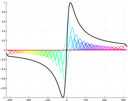
where $z=K_{l,i}^{t}A_{l}u_{t-1}$. In this study, we consider the linear combination of Gaussian Radial Basis Function (gRBF) for function approximation. Thus, the function $\phi_{l,i}^{t}$ is represented as

$$\phi_{l,i}^{t}(x)=\sum\nolimits_{j=1}^{M}w_{l,i,j}^{t}\varphi\left(\frac{|x-\mu_{j}|}{\gamma}\right)\,,$$ (3.6)

where $\varphi$ denotes the Gaussian kernel as shown in Fig. 3, $M$ is the number of basis kernels and $(\mu_{j},\gamma)$ is the center of the $j^{th}$ basis and the width, respectively. Therefore, the vector $\phi_{l,i}^{t}(z)$ can be reformulated via a matrix equation

$$\phi_{l,i}^{t}(z)=G(z)\cdot w_{l,i}^{t}\,,$$

where $w_{l,i}^{t}\in\mathbb{R}^{M}$ is the vectorized version of parameters $w_{l,i,j}^{t}$, matrix $G(z)\in\mathbb{R}^{O\times M}$ ($O$ is the number of pixels in $z$) is given as

$$\small\underbrace{\begin{bmatrix}\varphi(\frac{|z_{1}-\mu_{1}|}{\gamma})&\varphi(\frac{|z_{1}-\mu_{2}|}{\gamma})&\cdots&\varphi(\frac{|z_{1}-\mu_{M}|}{\gamma})\\ \varphi(\frac{|z_{2}-\mu_{1}|}{\gamma})&\varphi(\frac{|z_{2}-\mu_{2}|}{\gamma})&\cdots&\varphi(\frac{|z_{2}-\mu_{M}|}{\gamma})\\ \vdots&\vdots&\ddots&\vdots\\ \varphi(\frac{|z_{O}-\mu_{1}|}{\gamma})&\varphi(\frac{|z_{O}-\mu_{2}|}{\gamma})&\cdots&\varphi(\frac{|z_{O}-\mu_{M}|}{\gamma})\end{bmatrix}}_{\text{$G(z)$}}\underbrace{\left[\begin{array}[]{c}w_{l,i,1}\\ w_{l,i,2}\\ \vdots\\ w_{l,i,M}\end{array}\right]}_{\text{$w_{l,i}$}}=\underbrace{\left[\begin{array}[]{c}\phi_{l,i}\left(z_{1}\right)\\ \phi_{l,i}\left(z_{2}\right)\\ \vdots\\ \phi_{l,i}\left(z_{O}\right)\end{array}\right]}_{\text{$\phi_{l,i}(z)$}}\,.$$ (3.7)

Then, we can obtain the desired gradients of $u_{t}$ with respect to the influence function $\phi_{l,i}^{t}$, given as

$$\frac{\partial u_{t}}{\partial{\phi_{l,i}^{t}}}\triangleq\frac{\partial u_{t}}{\partial{w_{l,i}^{t}}}=-G^{\top}{\bar{K_{l,i}^{t}}}^{\top}A_{l}\,.$$ (3.8)

3.2.3 Computation of the derivatives of $\frac{\partial u_{t}}{\partial\lambda^{t}}$

From the diffusion model (3.3), it is easy to check that

$$\frac{\partial u_{t}}{\partial\lambda^{t}}=(u_{t-1}-f)^{\top}\,.$$ (3.9)

3.2.4 Computation of the derivatives of $\frac{\partial u_{t+1}}{\partial u_{t}}$

As pointed out in (2.5), in the joint training phase, we also need to compute $\frac{\partial u_{t+1}}{\partial u_{t}}$. This gradient can be obtained from the diffusion equation (3.3). The final formulation of $\frac{\partial u_{t+1}}{\partial u_{t}}$ is given as follows

$$\frac{\partial u_{t+1}}{\partial u_{t}}=(1-\lambda^{t+1})\mathbf{I}-\sum\nolimits_{l=0}^{L}\sum\limits_{i=1}^{N_{k}}A_{l}^{\top}\left({K_{l,i}^{t+1}}\right)^{\top}\cdot\Lambda_{l,i}\cdot\left({\bar{K}_{l,i}^{t+1}}\right)^{\top}A_{l}\,,$$ (3.10)

where $\Lambda_{l,i}$ is a diagonal matrix $\Lambda_{l,i}=\text{diag}({\phi_{l,i}^{t+1}}^{\prime}(z_{1}),\cdots,{\phi_{l,i}^{t+1}}^{\prime}(z_{p}))$ with $z=K_{l,i}^{t+1}A_{l}u_{t}$. Remember that the matrices $K_{l,i}^{t+1}$ and $\bar{K}_{l,i}^{t+1}$ are related to th linear kernels $k_{l,i}^{t+1}$ and $\bar{k}_{l,i}^{t+1}$, respectively.

3.3 Gradients for the case of Poisson denoising

3.3.1 Deriving the diffusion process for Poisson denoising

For the case of Poisson denoising, the data term should be chosen as

$$\lambda\langle u-f\mathrm{log}u,1\rangle\,,$$ (3.11)

with $u>0$. Casting it into the framework (3.2), we have two choices: (1) setting $\mathcal{D}(u,f)=\lambda\langle u-f\mathrm{log}u,1\rangle$ and $\mathcal{G}(u,f)=0$; (2) setting $\mathcal{D}(u,f)=0$ and $\mathcal{G}(u,f)=\lambda\langle u-f\mathrm{log}u,1\rangle$.

Considering the first setup, we have $\phi(u,f)=\nabla_{u}\mathcal{D}(u,f)=\lambda(1-\frac{f}{u})$. One can see that, this strategy is not applicable in practice, because (a) it has an evident problem of numerical instability at the points where $u$ is very close to zero; (b) this update rule can not guarantee that the output image after one diffusion step is positive. Negative values of $u$ will violate the constraint of the data term (3.11).

Then we resort to the second strategy by setting $\mathcal{D}(u,f)=0$ and $\mathcal{G}(u,f)=\lambda\langle u-f\mathrm{log}u,1\rangle$. The proximal mapping with respect to $\mathcal{G}$ is given as the following minimization problem

$$\left(\mathbf{I}+\partial\mathcal{G}\right)^{-1}(\tilde{u})=\arg\min\limits_{u}\frac{\|u-\tilde{u}\|^{2}_{2}}{2}+\lambda\langle u-f\mathrm{log}u,1\rangle\,.$$ (3.12)

The solution of (3.12) is given by the following point-wise operation

$$\hat{u}=\left(\mathbf{I}+\partial\mathcal{G}\right)^{-1}(\tilde{u})=\frac{\tilde{u}-\lambda+\sqrt{\left(\tilde{u}-\lambda\right)^{2}+4\lambda f}}{2}\,.$$ (3.13)

Note that $\hat{u}$ is always positive if $f>0$, i.e, this update rule can guarantee $\hat{u}>0$ in diffusion steps.

As a consequence, the diffusion process for Poisson denoising using the proximal gradient method is formulated as

$$u_{t+1}=\frac{\tilde{u}_{t+1}-\lambda^{t+1}+\sqrt{\left(\tilde{u}_{t+1}-\lambda^{t+1}\right)^{2}+4\lambda^{t+1}f}}{2}\,,$$ (3.14)

where $\tilde{u}_{t+1}=u_{t}-\sum\limits_{l=0}^{L}\sum\limits_{i=1}^{N_{k}}A_{l}^{\top}\left(\bar{k}_{l,i}^{t+1}*\phi_{l,i}^{t+1}(k_{l,i}^{t+1}*A_{l}u_{t})\right)$.

3.4 Computing the gradients for training

Following the results presented in the previous subsection, for the training phase, we mainly need to compute $\frac{\partial u_{t+1}}{\partial u_{t}}$ and $\frac{\partial u_{t}}{\partial\Theta_{t}}$.

Based on the diffusion procedure (3.14), $\frac{\partial u_{t+1}}{\partial u_{t}}$ is computed via the chain rule, given as

$$\frac{\partial u_{t+1}}{\partial u_{t}}=\frac{\partial\tilde{u}_{t+1}}{\partial u_{t}}\cdot\frac{\partial u_{t+1}}{\partial\tilde{u}_{t+1}}.$$ (3.15)

$\frac{\partial\tilde{u}_{t+1}}{\partial u_{t}}$ can be easily obtained by following the result (3.10). Concerning the part $\frac{\partial u_{t+1}}{\partial\tilde{u}_{t+1}}$, it can be computed according to (3.14) and is formulated as

$$\frac{\partial u_{t+1}}{\partial\tilde{u}_{t+1}}=\text{diag}(y_{1},\cdots,y_{N})\,,$$ (3.16)

where $\{y_{i}\}_{i=1}^{i=N}$ denote the elements of

$$y=\frac{1}{2}\left[1+\frac{\tilde{u}_{t+1}-\lambda^{t+1}}{\sqrt{\left(\tilde{u}_{t+1}-\lambda^{t+1}\right)^{2}+4\lambda^{t+1}f}}\right]\,.$$

Concerning the gradients $\frac{\partial u_{t}}{\partial\Theta_{t}}$ ($\Theta_{t}$ involves $\left\{\lambda^{t},\phi_{l,i}^{t},k_{l,i}^{t}\right\}$), it is worthy noting that the gradients of $u_{t}$ with respect to $\left\{\phi_{l,i}^{t},k_{l,i}^{t}\right\}$ are only associated with

$$\tilde{u}_{t}=u_{t-1}-\sum\limits_{l=0}^{L}\sum\limits_{i=1}^{N_{k}}A_{l}^{\top}\left(\bar{k}_{l,i}^{t}*\phi_{l,i}^{t}(k_{l,i}^{t}*A_{l}u_{t-1})\right)\,.$$

Therefore, the gradient of $u_{t}$ with respect to $\phi_{l,i}^{t}$ and $k_{l,i}^{t}$ is computed via

$$\frac{\partial u_{t}}{\partial\phi_{l,i}^{t}}=\frac{\partial\tilde{u}_{t}}{\partial\phi_{l,i}^{t}}\cdot\frac{\partial u_{t}}{\partial\tilde{u}_{t}},\,\mathrm{and}\,\,\frac{\partial u_{t}}{\partial k_{l,i}^{t}}=\frac{\partial\tilde{u}_{t}}{\partial k_{l,i}^{t}}\cdot\frac{\partial u_{t}}{\partial\tilde{u}_{t}},$$

where the derivations of $\frac{\partial\tilde{u}_{t}}{\partial\phi_{l,i}^{t}}$ and $\frac{\partial\tilde{u}_{t}}{\partial k_{l,i}^{t}}$ are given as (3.8) and (3.4), respectively. The gradients of $\frac{\partial u_{t}}{\partial\tilde{u}_{t}}$ are calculated similar to (3.16).

The gradient of $u_{t}$ with respect to $\lambda^{t}$ is computed as

$$\frac{\partial u_{t}}{\partial\lambda^{t}}=(z_{1},\cdots,z_{N})\,,$$ (3.17)

where $\{z_{i}\}_{i=1}^{i=N}$ denote the elements of

$$z=\frac{1}{2}\left[-1+\frac{\left(\lambda^{t}-\tilde{u}_{t}\right)+2f}{\sqrt{\left(\tilde{u}_{t}-\lambda^{t}\right)^{2}+4\lambda^{t}f}}\right]\,.$$

Note that $\frac{\partial u_{t}}{\partial\lambda^{t}}$ is written as a row vector.

4 Experiments

In this section, we employed the fully Trained Multi-scale Nonlinear Diffusion Model (MSND) for Gaussian denoising and Poisson Denoising. The corresponding nonlinear diffusion process of stage $T$ with filters of size $m\times m$ is expressed as $\mathrm{MSND}_{m\times m}^{T}$. Note that there are different options for the number of scales. It is not a stretch to infer that more scales leads to better denoising performance, but increases the cost of computing. Without loss of generality, in this study we employed three scales with the scale factors 1.5, 2 and 3 respectively. The number of filters for each scale is $\left(m^{2}-1\right)$ in each stage, if not specified.

To generate the training data for our denoising experiments, we cropped a 180$\times$180 pixel region from each image of the Berkeley segmentation dataset [26], resulting in a total of 400 training samples of size 180 $\times$ 180. This setting is the same as TNRD [8] for fair evaluation. After training the models, we evaluated them on 68 test images originally introduced by [33], which have since become a reference set for image denoising. To provide a comprehensive comparison, the standard deviations $\sigma$ for the Gaussian noise are set as 25, 50, 75 and 100, respectively. Meanwhile, the peak values of Poisson noise are distributed between 1 to 4. For saving the training time, the $\mathrm{MSND}_{7\times 7}^{5}$ model is employed. Meanwhile, we also tested the $\mathrm{MSND}_{5\times 5}^{5}$ model for comparison. Note that, the diffusion model needs to be trained respectively for different noise levels and different noise types.

(a) Clean Image $I_{0}$

(b) Noisy image $I_{m}$. $\sigma=50$

(c) The under-sampled noisy image $I_{m}^{1.5}$.

(d) The under-sampled noisy image $I_{m}^{2}$.

(e) The under-sampled noisy image $I_{m}^{3}$.

(f) $\mathrm{TNRD}_{5\times 5}^{5}$ (37.46/0.952)

(g) $\mathrm{TNRD}_{7\times 7}^{5}$ (39.22/0.970)

(h) $\mathrm{MSND}_{5\times 5}^{5}$ (41.34/0.976)

(i) $\mathrm{MSND}_{7\times 7}^{5}$ (43.64/0.985)

Figure 4: Denoising results comparison. The results are reported by PSNR/SSIM index. Best results are marked. Note that the under-sampled noisy image $I_{m}^{n}$ is obtained by sub-sampling $I_{m}$ with scale factor $n$. The resulting standard deviation is $\sigma=\frac{50}{n}$.

For Gaussian denoising task, the proposed algorithm is compared with five representative state-of-the-art methods: BM3D [11], WNNM [14], EPLL-GMM [43], multi-scale EPLL-GMM(MSEPLL) [29] and TNRD [8]. For Poisson noise denoising, we compared with the NLSPCA [35] and BM3D-based methods with the exact unbiased inverse Anscombe [25], both with and without binning technique. The corresponding codes are downloaded from the authors’ homepage, and we used them as is. Especially, for the binning technique in the Poisson denoising task, we closely followed [35] and use a $3\times 3$ ones kernel to increase the peak value to be 9 times higher, and a bilinear interpolation for the upscaling of the low-resolution recovered image. Two commonly used quality measures are taken to evaluate the denoising performance, i.e., PSNR and the structural similarity index (SSIM) [39]. The range of SSIM value lies in [0, 1] with 1 standing for perfect quality. The PSNR and SSIM values in the following subsections are evaluated by averaging denoised results of 68 test images. Note that the PSNR value for Poisson noise denoising is computed based on the peak value, instead of 255 for Gaussian noise denosing task on 8-bit images.

4.1 Gaussian Denoising

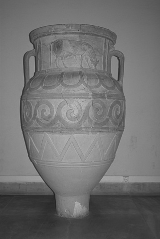
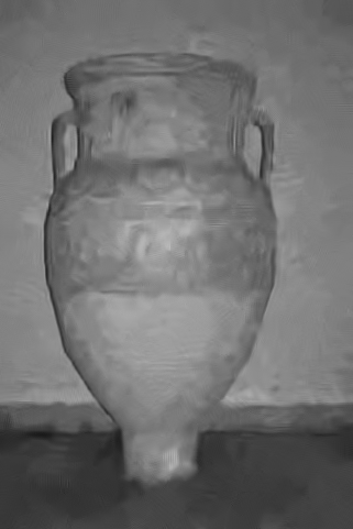
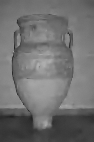
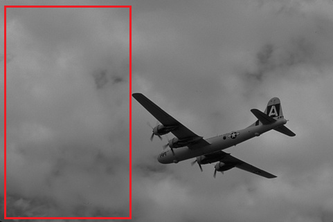
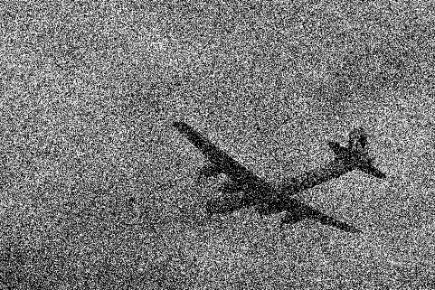
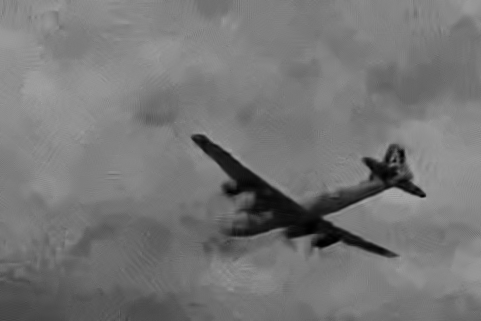
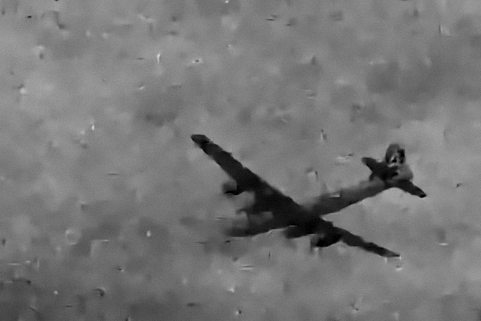
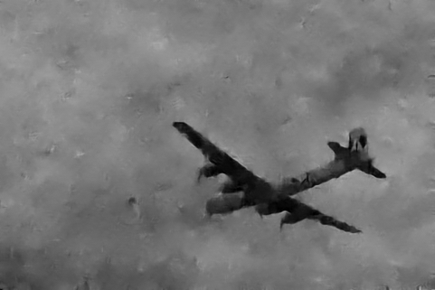
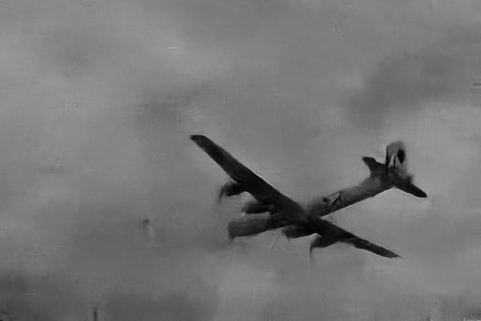
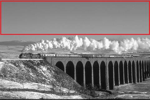
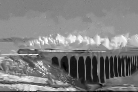
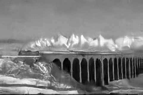
The main motivation for constructing a multi-scale model was to remedy the artifacts obtained from local processing of the image. Therefore, we begin with a preliminary test in Fig. 4 which presents the denoised images obtained by the local model TNRD [8] and the proposed model, showing that indeed artifacts are better treated. In detail, by observing on the recovered images, we can see that the single-scale local model TNRD introduces some incorrect image features. This is because that local models infer the underlying structure solely from the local neighborhoods, which is heavily distorted by noise. In this case, the advantage of multi-scale structure comes through.

The downsampling operation in the proposed multi-scale model MSND can cause the uncorrelated values of the noise to become smaller and consequently make image structures more visible, as shown in Fig. 4(c), (d) and (e). Moreover, down-sampling the image before denoising amounts to enlarging the size of the neighborhood on which the denoising is performed, thus permitting to exploit larger-scale information. As a consequence, the proposed multi-scale model MSND leads to great performance improvements by comparing Fig. 4(f,g) with (h,i).

(a) Clean Image

(b) Noisy image. $\sigma=50$

(c) BM3D(30.71/0.790)

(d) EPLL(30.12/0.763)

(e) WSEPLL(30.87/0.794)

(f) WNNM(30.68/0.790)

(g) $\mathrm{TNRD}_{5\times 5}^{5}$ (30.38/0.775)

(h) $\mathrm{TNRD}_{7\times 7}^{5}$ (30.63/0.785)

(i) $\mathrm{MSND}_{5\times 5}^{5}$ (30.79/0.789)

(j) $\mathrm{MSND}_{7\times 7}^{5}$ (30.95/0.794)

Figure 5: Gaussian noise denoising results comparison. The results are reported by PSNR/SSIM index. Best results are marked.

(a) Clean Image

(b) Noisy image. $\sigma=75$

(c) BM3D(31.32/0.899)

(d) EPLL(30.14/0.831)

(e) WSEPLL(32.05/0.927)

(f) WNNM(31.53/0.913)

(g) $\mathrm{TNRD}_{5\times 5}^{5}$ (31.28/0.894)

(h) $\mathrm{TNRD}_{7\times 7}^{5}$ (31.85/0.911)

(i) $\mathrm{MSND}_{5\times 5}^{5}$ (32.31/0.919)

(j) $\mathrm{MSND}_{7\times 7}^{5}$ (32.61/0.928)

Figure 6: Gaussian noise denoising results comparison. The results are reported by PSNR/SSIM index. Best results are marked.

(a) Clean Image

(b) Noisy image. $\sigma=100$

(c) BM3D(21.85/0.650)

(d) EPLL(21.54/0.594)

(e) WSEPLL(21.70/0.641)

(f) WNNM(22.08/0.671)

(g) $\mathrm{TNRD}_{5\times 5}^{5}$ (21.67/0.636)

(h) $\mathrm{TNRD}_{7\times 7}^{5}$ (21.87/0.659)

(i) $\mathrm{MSND}_{5\times 5}^{5}$ (22.01/0.671)

(j) $\mathrm{MSND}_{7\times 7}^{5}$ (22.07/0.683)

Figure 7: Gaussian noise denoising results comparison. The results are reported by PSNR/SSIM index. Best results are marked.

Method	$\sigma=25$	$\sigma=50$	$\sigma=75$	$\sigma=100$
BM3D	28.57/0.802	25.62/0.687	24.21/0.622	23.24/0.576
EPLL	28.68/0.812	25.68/0.688	24.10/0.606	23.06/ 0.547
MSEPLL	28.78/0.812	25.83/0.692	24.30/0.620	23.32/0.573
WNNM	28.80/0.808	25.83/0.698	24.39/ 0.626	23.39/0.585
$\mathrm{TNRD}_{5\times 5}^{5}$	28.77/0.808	25.83/0.692	24.33/0.624	23.30/0.574
$\mathrm{TNRD}_{7\times 7}^{5}$	28.93/0.816	25.96/0.702	24.45/0.632	23.47/0.586
$\mathrm{MSND}_{5\times 5}^{5}$	28.92/0.815	26.01/0.704	24.54/0.638	23.58/0.593
$\mathrm{MSND}_{7\times 7}^{5}$	28.98/0.820	26.06/0.709	24.58/0.642	23.62/0.598

Table 1: Comparison of the performance on the Gaussian noise denoising of the test algorithms in terms of PSNR and SSIM. Best results are marked.

(a) $\sigma=50$, the filter size is $5\times 5$

(b) $\sigma=75$, the filter size is $5\times 5$

(c) $\sigma=50$, the filter size is $7\times 7$

(d) $\sigma=75$, the filter size is $7\times 7$

Figure 8: Scatter plot of the PSNRs over 68 test images produced by the proposed MSND model, BM3D, WNNM, MSEPLL and TNRD. A point above the diagonal line (i.e., $y=x$) means a better performance than the proposed model, and a point below this line indicates a inferior result. One can see that the proposed MSND model outperforms the other test methods on most of the images.

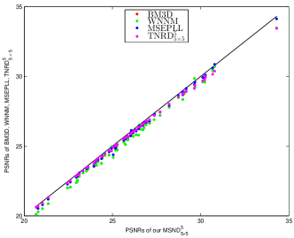
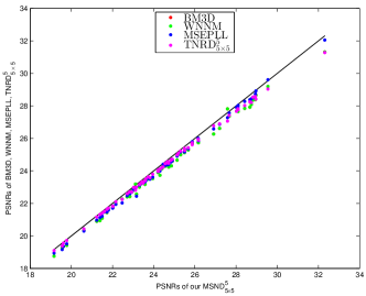
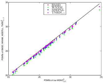
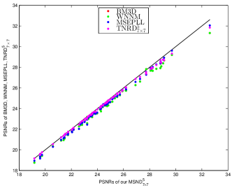
Examining the recovery images in Fig. 5-Fig. 7, the nonlocal technique BM3D is affected by the structured signal-like artifacts that appear in homogeneous areas of the image. This phenomenon is originated from the selection process of similar image patches in the BM3D denoising scheme. The selection process is easily influenced by the noise itself, especially in flat areas of the image, which can be dangerously self-referential. Meanwhile, we find that the method TNRD introduces block-type artifacts, whose reason has been explained above. In comparison with TNRD, the proposed algorithm MSND is more powerful on suppressing artifacts and recovering the homogeneous regions of the image, especially within the red rectangles in the presented figures.

The recovery errors in terms of PSNR (in dB) and SSIM are summarized in Table 1. Comparing the indexes in Table 1 and the denoising results in the present figures, the best overall performance is provided by the proposed method MSND. Especially, with the noise level increasing, the superiority of MSND enhances as well. This is natural since the artifacts brought by the single-scale local model are more serious when the noise level is higher. Meanwhile, the proposed model not only leads to an improvement in smooth regions, but also performs at least as well as the single-scale local model in highly textured areas.

Fig. 8 presents a detailed comparison between our learned MSND model and four state-of-the-art methods over 68 natural images for noise level $\sigma$ = 50 and $\sigma$ = 75. One can see that our proposed MSND outperforms the compared denoising methods for most images.

4.2 Poisson Denoising

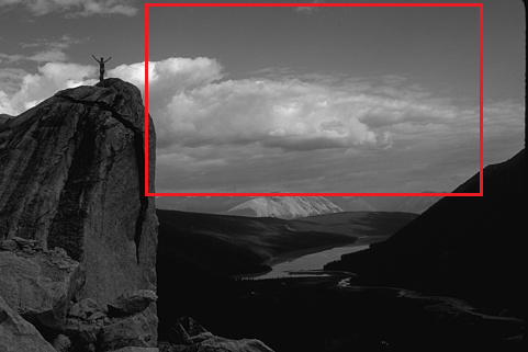
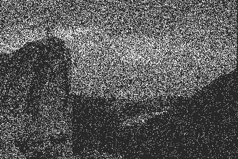
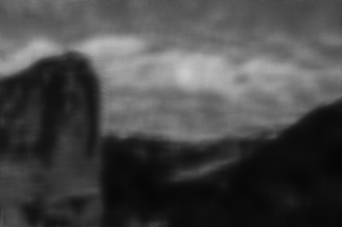
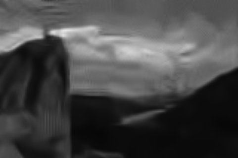
Overall speaking, the denoising performance for Poisson noise denoising is consistent with the Gaussian case. It is worthy noting that the BM3D-based method without binning brings in the typical structured artifacts especially in smooth areas. However, the binning technique yields noisy images with lower noise level, thereby the denoised results in this case is less disturbed by the structured signal-like artifacts. But the adoption of the binning technique leads to resolution reduction which will weaken or even eliminate many image details. In the visual quality, the typical structured artifacts encountered with the single-scale local model do not appear when the proposed method MSND is used, which can noticeably be visually perceived by the comparison in Fig. 9-Fig. 11.

(a) Clean Image

(b) Noisy image. Peak=1

(c) NLSPCA (25.78/0.717)

(d) NLSPCAbin (23.72/0.715)

(e) BM3D (25.51/0.714)

(f) BM3Dbin (26.22/0.738)

(g) $\mathrm{TNRD}_{5\times 5}^{5}$ (26.02/0.675)

(h) $\mathrm{TNRD}_{7\times 7}^{5}$ (26.29/0.690)

(i) $\mathrm{MSND}_{5\times 5}^{5}$ (26.47/0.706)

(j) $\mathrm{MSND}_{7\times 7}^{5}$ (26.65/0.714)

Figure 9: Poisson noise denoising results comparison. The results are reported by PSNR/SSIM index. Best results are marked.

(a) Clean Image

(b) Noisy image. Peak=2

(c) NLSPCA (21.11/0.613)

(d) NLSPCAbin (20.30/0.606)

(e) BM3D (22.03/0.627)

(f) BM3Dbin (21.99/0.643)

(g) $\mathrm{TNRD}_{5\times 5}^{5}$ (22.40/0.623)

(h) $\mathrm{TNRD}_{7\times 7}^{5}$ (22.51/0.640)

(i) $\mathrm{MSND}_{5\times 5}^{5}$ (22.77/0.656)

(j) $\mathrm{MSND}_{7\times 7}^{5}$ (22.84/0.662)

Figure 10: Poisson noise denoising results comparison. The results are reported by PSNR/SSIM index. Best results are marked.

(a) Clean Image

(b) Noisy image. Peak=4

(c) NLSPCA (26.04/0.764)

(d) NLSPCAbin (22.94/0.724)

(e) BM3D (26.27/0.684)

(f) BM3Dbin (27.08/0.780)

(g) $\mathrm{TNRD}_{5\times 5}^{5}$ (27.01/0.738)

(h) $\mathrm{TNRD}_{7\times 7}^{5}$ (27.46/0.762)

(i) $\mathrm{MSND}_{5\times 5}^{5}$ (27.72/0.774)

(j) $\mathrm{MSND}_{7\times 7}^{5}$ (27.85/0.784)

Figure 11: Poisson noise denoising results comparison. The results are reported by PSNR/SSIM index. Best results are marked.

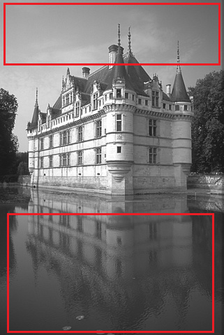
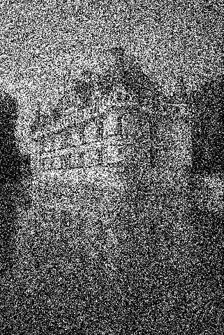
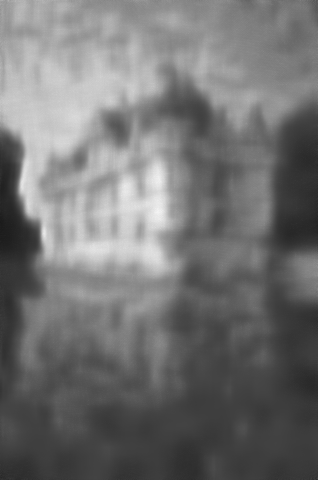
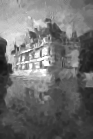
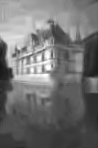
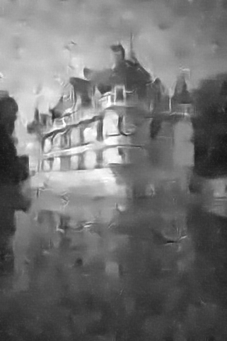
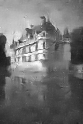
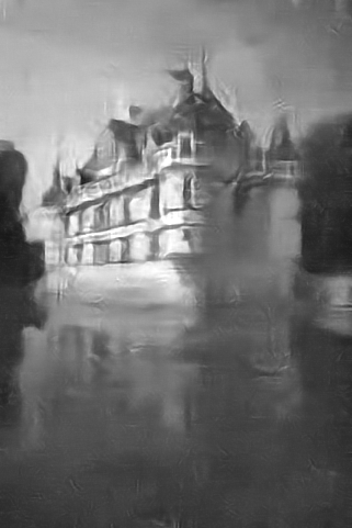
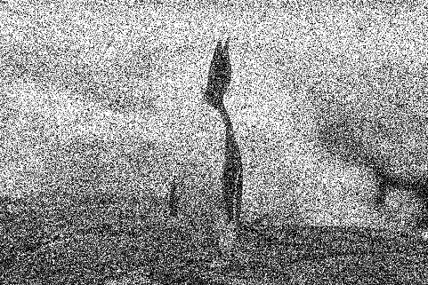
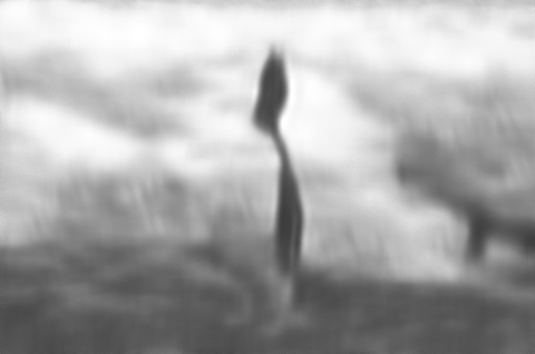
Overall speaking, the performance of MSND in terms of PSNR/SSIM is better than the other methods, as shown in Table 2. This indicates that for most images our method is more powerful in the recover quality and geometry feature preservation.

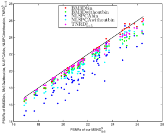
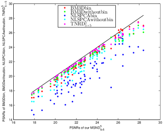
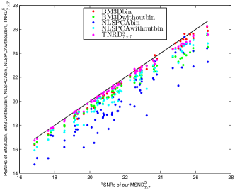
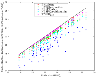
Figure 12 presents a detailed comparison between our learned MSND model and four state-of-the-art methods over 68 natural images for noise level peak = 1 and peak = 2, where the diagonal line $y=x$ means an equal performance to ours. One can see that our method performs better for most images.

Method	Peak=1	Peak=2	Peak=4
NLSPCA	20.90/0.491	21.60/0.517	22.09/0.535
NLSPCAbin	19.89/0.466	19.95/0.467	19.95/0.467
BM3D	21.01/0.504	22.21/0.544	23.54/0.604
BM3Dbin	21.39/0.515	22.14/0.542	22.87/0.571
$\mathrm{TNRD}_{5\times 5}^{5}$	21.34/0.497	22.45/0.548	23.58/0.603
$\mathrm{TNRD}_{7\times 7}^{5}$	21.53/0.511	22.59/0.557	23.80/0.615
$\mathrm{MSND}_{5\times 5}^{5}$	21.71/0.523	22.78/0.568	23.89/0.620
$\mathrm{MSND}_{7\times 7}^{5}$	21.76/0.526	22.83/0.573	23.94/0.625

Table 2: Comparison of the performance on Poisson denoising of the test algorithms in terms of PSNR and SSIM. Best results are marked.

(a) peak=1, the filter size is $5\times 5$

(b) peak=2, the filter size is $5\times 5$

(c) peak=1, the filter size is $7\times 7$

(d) peak=2, the filter size is $7\times 7$

Figure 12: Scatter plot of the PSNRs over 68 test images produced by the proposed MSND model, BM3Dbin, BM3Dwithoutbin, NLSPCAbin, NLSPCAwithoutbin and TNRD. A point above the diagonal line (i.e., $y=x$) means a better performance than the proposed model, and a point below this line indicates a inferior result. One can see that the proposed MSND model outperforms the other methods on almost all test images.

4.3 Run Time

	BM3D	WNNM	EPLL	MSEPLL	$\mathrm{TNRD}_{5\times 5}^{5}$	$\mathrm{TNRD}_{7\times 7}^{5}$	$\mathrm{MSND}_{5\times 5}^{5}$	$\mathrm{MSND}_{7\times 7}^{5}$
$256\times 256$	1.38	154.2	62.9	226.1	0.63 (0.006)	1.48 (0.013)	1.62 (0.015)	3.76 (0.028)
$512\times 512$	4.6	612.8	257.6	895.7	1.90 (0.018)	4.61 (0.043)	4.77 (0.043)	11.04 (0.101)

Table 3: Typical run time (in second) of the Gaussian denoising methods for images with two different dimensions. The CPU computation time is evaluated on Intel CPU X5675, 3.07GHz. The highlighted number is the run time of GPU implementation based on NVIDIA Geforce GTX 780Ti.

	BM3D	NLSPCA	$\mathrm{TNRD}_{5\times 5}^{5}$	$\mathrm{TNRD}_{7\times 7}^{5}$	$\mathrm{MSND}_{5\times 5}^{5}$	$\mathrm{MSND}_{7\times 7}^{5}$
$256\times 256$	1.38	367.9	0.65 (0.006)	1.52 (0.013)	1.63 (0.015)	3.80 (0.029)
$512\times 512$	4.6	1122.1	1.92 (0.019)	4.66 (0.044)	4.80 (0.043)	11.06 (0.101)

Table 4: Typical run time (in second) of the Poisson denoising methods for images with two different dimensions. The CPU computation time is evaluated on Intel CPU X5675, 3.07GHz. The highlighted number is the run time of GPU implementation based on NVIDIA Geforce GTX 780Ti.

It is worthwhile to note that the proposed model is as efficient as TNRD, and merely contains convolution of linear filters with an image, which offers high levels of parallelism making it well suited for GPU implementation.

Table 3 and Table 4 report the typical run time of the proposed model for the images of two different dimensions for the case of Gaussian denoising and Poisson denoising. We also present the run time of several competing algorithms.

Due to the structural simplicity of the proposed model, it is well-suited to GPU parallel computation. We are able to implement our algorithm on GPU with ease. It turns out that the GPU implementation based on NVIDIA Geforce GTX 780Ti can accelerate the inference procedure significantly, as shown in Table 3 and Table 4. By comparison, we see that the proposed MSND model is generally competitive with the other test methods, especially another multi-scale scheme MSEPLL.

5 Conclusion

In this study we employed the multi-scale pyramid image representation to devise a multi-scale nonlinear diffusion process. The proposed model can efficiently suppress the typical noise artifacts brought by the single-scale local model, especially when the noise level is relatively high. All the parameters in the proposed multi-scale diffusion model, including the filters and the influence functions across scales, are learned from training data through a loss based approach. Numerical results on Gaussian and Poisson denoising substantiate that the exploited multi-scale strategy can successfully boost the performance of the original TNRD model with single scale. As a consequence, the resulting multi-scale diffusion models can significantly suppress the typical incorrect features for those noisy images with heavy noise. Based on standard test dataset, the proposed multi-scale nonlinear diffusion model provides strongly competitive results against state-of-the-art approaches. Moreover, the proposed model bears the properties of simple structure and high efficiency, therefore is well suited to GPU computing. Our future study can be generalization of the proposed multi-scale model into some other image restoration tasks such as deblurring, super-resolution and so on.

References

- [1] Codruta O Ancuti and Cosmin Ancuti. Single image dehazing by multi-scale fusion. Image Processing, IEEE Transactions on, 22(8):3271–3282, 2013.
- [2] Jake Bouvrie. Notes on convolutional neural networks. 2006.
- [3] Harold C Burger, Christian J Schuler, and Stefan Harmeling. Image denoising: Can plain neural networks compete with BM3D? In CVPR, pages 2392–2399, 2012.
- [4] Harold Christopher Burger and Stefan Harmeling. Improving denoising algorithms via a multi-scale meta-procedure. In DAGM, pages 206–215. 2011.
- [5] S Grace Chang, Bin Yu, and Martin Vetterli. Adaptive wavelet thresholding for image denoising and compression. Image Processing, IEEE Transactions on, 9(9):1532–1546, 2000.
- [6] Priyam Chatterjee and Peyman Milanfar. Is denoising dead? Image Processing, IEEE Transactions on, 19(4):895–911, 2010.
- [7] Yunjin Chen, René Ranftl, and Thomas Pock. Insights into analysis operator learning: From patch-based sparse models to higher order mrfs. Image Processing, IEEE Transactions on, 23(3):1060–1072, 2014.
- [8] Yunjin Chen, Wei Yu, and Thomas Pock. On learning optimized reaction diffusion processes for effective image restoration. In Proc. IEEE Conference on Computer Vision and Pattern Recognition (CVPR), 2015.
- [9] Davide Cozzolino, Sara Parrilli, Giuseppe Scarpa, Giovanni Poggi, and Luisa Verdoliva. Fast adaptive nonlocal SAR despeckling. Geoscience and Remote Sensing Letters, IEEE, 11(2):524–528, 2014.
- [10] Imre Csiszár. Why least squares and maximum entropy? an axiomatic approach to inference for linear inverse problems. The Annals of Statistics, 19(4):2032–2066, 1991.
- [11] Kostadin Dabov, Alessandro Foi, Vladimir Katkovnik, and Karen Egiazarian. Image denoising by sparse 3-d transform-domain collaborative filtering. Image Processing, IEEE Transactions on, 16(8):2080–2095, 2007.
- [12] Michael Elad and Michal Aharon. Image denoising via sparse and redundant representations over learned dictionaries. Image Processing, IEEE Transactions on, 15(12):3736–3745, 2006.
- [13] Raja Giryes and Michael Elad. Sparsity-based poisson denoising with dictionary learning. Image Processing, IEEE Transactions on, 23(12):5057–5069, 2014.
- [14] Shuhang Gu, Lei Zhang, Wangmeng Zuo, and Xiangchu Feng. Weighted nuclear norm minimization with application to image denoising. In CVPR, pages 2862–2869, 2014.
- [15] Viren Jain and Sebastian Seung. Natural image denoising with convolutional networks. In NIPS, pages 769–776, 2009.
- [16] Xudong Kang, Shutao Li, and Jon Atli Benediktsson. Spectral–spatial hyperspectral image classification with edge-preserving filtering. Geoscience and Remote Sensing, IEEE Transactions on, 52(5):2666–2677, 2014.
- [17] Triet Le, Rick Chartrand, and Thomas J Asaki. A variational approach to reconstructing images corrupted by Poisson noise. Journal of Mathematical Imaging and Vision, 27(3):257–263, 2007.
- [18] Marc Lebrun, Miguel Colom, and Jean-Michel Morel. Multiscale image blind denoising. Image Processing, IEEE Transactions on, 24(10):3149–3161, 2015.
- [19] Yann LeCun, Léon Bottou, Yoshua Bengio, and Patrick Haffner. Gradient-based learning applied to document recognition. Proceedings of the IEEE, 86(11):2278–2324, 1998.
- [20] Stamatios Lefkimmiatis, Petros Maragos, and George Papandreou. Bayesian inference on multiscale models for poisson intensity estimation: applications to photon-limited image denoising. Image Processing, IEEE Transactions on, 18(8):1724–1741, 2009.
- [21] D. C. Liu and J. Nocedal. On the limited memory BFGS method for large scale optimization. Mathematical Programming, 45(1):503–528, 1989.
- [22] Xianming Liu, Deming Zhai, Debin Zhao, Guangtao Zhai, and Wen Gao. Progressive image denoising through hybrid graph laplacian regularization: a unified framework. Image Processing, IEEE Transactions on, 23(4):1491–1503, 2014.
- [23] Xiaobai Liu, Qian Xu, Jiayi Ma, Hai Jin, and Yanduo Zhang. MsLRR: A unified multiscale low-rank representation for image segmentation. Image Processing, IEEE Transactions on, 23(5):2159–2167, 2014.
- [24] Julien Mairal, Francis Bach, Jean Ponce, Guillermo Sapiro, and Andrew Zisserman. Non-local sparse models for image restoration. In ICCV, pages 2272–2279, 2009.
- [25] Markku Makitalo and Alessandro Foi. Optimal inversion of the Anscombe transformation in low-count Poisson image denoising. IEEE Trans. Image Process., 20(1):99–109, 2011.
- [26] D. Martin, C. Fowlkes, D. Tal, and J. Malik. A database of human segmented natural images and its application to evaluating segmentation algorithms and measuring ecological statistics. In Proc. 8th Int’l Conf. Computer Vision, volume 2, pages 416–423, July 2001.
- [27] Vinod Nair and Geoffrey E Hinton. Rectified linear units improve restricted boltzmann machines. In Proc. IEEE Int’l Conf. Machine Learning, pages 807–814, 2010.
- [28] Yu. Nesterov. Introductory lectures on convex optimization, volume 87 of Applied Optimization. Kluwer Academic Publishers, Boston, MA, 2004. A basic course.
- [29] Vardan Papyan and Michael Elad. Multi-scale patch-based image restoration. Image Processing, IEEE Transactions on, 25(1):249–261, 2016.
- [30] Sara Parrilli, Mariana Poderico, Cesario Vincenzo Angelino, and Luisa Verdoliva. A nonlocal SAR image denoising algorithm based on LLMMSE wavelet shrinkage. Geoscience and Remote Sensing, IEEE Transactions on, 50(2):606–616, 2012.
- [31] Pietro Perona and Jitendra Malik. Scale-space and edge detection using anisotropic diffusion. Pattern Analysis and Machine Intelligence, IEEE Transactions on, 12(7):629–639, 1990.
- [32] Javier Portilla, Vasily Strela, Martin J Wainwright, and Eero P Simoncelli. Image denoising using scale mixtures of gaussians in the wavelet domain. Image Processing, IEEE Transactions on, 12(11):1338–1351, 2003.
- [33] Stefan Roth and Michael J Black. Fields of experts. International Journal of Computer Vision, 82(2):205–229, 2009.
- [34] Leonid I Rudin, Stanley Osher, and Emad Fatemi. Nonlinear total variation based noise removal algorithms. Physica D: Nonlinear Phenomena, 60(1):259–268, 1992.
- [35] Joseph Salmon, Zachary Harmany, Charles-Alban Deledalle, and Rebecca Willett. Poisson noise reduction with non-local PCA. Journal of mathematical imaging and vision, 48(2):279–294, 2014.
- [36] Uwe Schmidt and Stefan Roth. Shrinkage fields for effective image restoration. In CVPR, pages 2774–2781, 2014.
- [37] Heidarali Talebi and Peyman Milanfar. Global image denoising. Image Processing, IEEE Transactions on, 23(2):755–768, 2014.
- [38] Yuan-Kai Wang and Ching-Tang Fan. Single image defogging by multiscale depth fusion. Image Processing, IEEE Transactions on, 23(11):4826–4837, 2014.
- [39] Zhou Wang, Alan C Bovik, Hamid R Sheikh, and Eero P Simoncelli. Image quality assessment: from error visibility to structural similarity. IEEE Trans. Image Process., 13(4):600–612, 2004.
- [40] Max Welling, Simon Osindero, and Geoffrey E Hinton. Learning sparse topographic representations with products of student-t distributions. In NIPS, pages 1359–1366, 2002.
- [41] Huanjing Yue, Xiaoyan Sun, Jingyu Yang, and Feng Wu. Image denoising by exploring external and internal correlations. Image Processing, IEEE Transactions on, 24(6):1967–1982, 2015.
- [42] Maria Zontak, Inbar Mosseri, and Michal Irani. Separating signal from noise using patch recurrence across scales. In CVPR, pages 1195–1202, 2013.
- [43] Daniel Zoran and Yair Weiss. From learning models of natural image patches to whole image restoration. In ICCV, pages 479–486, 2011.