How To Build A Quantum Coherent Observer

Abstract

We give an explicit construction for a quantum observer coherently mimicking the dynamics of a cavity mode system and without any disturbance of the system’s dynamics. This gives the exact analogue of the Luenberger observer used in controller design in engineering.

I Introduction

In this letter we wish to discuss an engineering-oriented aspect of the quantum observers. In control theory, an observer is a dynamical system capable of mimicking the dynamical state of a given system (known as the plant): it should have the same class of state variables and these variables should become close in the asymptotic long-time limit. The concept was introduced by Luenberger Luenberger64 ,Luenberger66 and plays an important role in controller design. In the quantum setting, an observer receives information about the system. This can happen when the observer is making continuous measurements on a quantum system and then deriving the conditioned state of system using a quantum filter (quantum trajectories). In many cases a quantum control problem can be broken down by a separation principle BvH_sep into a measurement stage and an actuation stage.

However, our interest is in quantum coherent observers. Here we mean a quantum system that is coupled to the quantum (plant) system of interest and which has capable of realizing a model of the plant’s dynamics internally and where this internal observer dynamics converges to that of the plant. The concept was introduced in Zibo12 and developed as a conceptual device for quantum design Zibo_16 -Pan16 . In these approaches, one considers the observer embedded in a quantum feedback network with connections to the plant system in such a way that there is a feedback loop between the plant and observer - moreover the observer is then part of the controller design problem. We wish to avoid this and have the plant feedforward information to the observer - but not the other way round. In this manner, there is no back-action of the observer on the plant - more exactly, as no measurement need be involved, we mean that the plant’s dynamics is not modified by connection to the observer. Our construction, given below, is based on the original Luenberger set-up and the quantization is done by replacing the classical block design with a quantum feedback network where the plant and observer are quantum linear systems and where jump-off and summing junctions are replaced with beam-splitters.

I.1 Classical Luenberger Observers

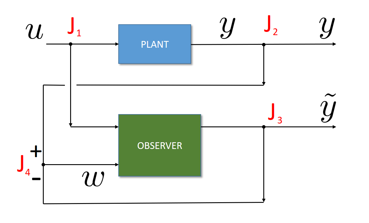
The set up for a classical Luenberger observer is sketched in Figure 1 which shows a plant system with input $u$ and output $y$ connected to a second system which we term the observer.

Figure 1: A Luenberger observer connected to a plant system.

The plant is taken to be a linear system with the input-state-output equations

$$\dot{x} = Ax+Bu,$$

$$y = Cx.$$ (1)

What we wish to do is to have the observer track the state $x$ of the plant system. The observer is also taken to be a linear system with state $\tilde{x}$, input $y$ and $w$ and output $\tilde{y}$ and input-state-output equations

$$\dot{\tilde{x}} = A\tilde{x}+Bu+Lw,$$

$$\tilde{y} = C\tilde{x}.$$ (2)

Note that the same coefficients $A,B,C$ occur in both the plant and observer models. The additional coefficient $L$ in the observer is called the Luenberger gain.

In the set-up we require 4 junctions: $J_{1},J_{2},J_{3}$ are jump points where we copy the signals $u$, $y$ and $\tilde{y}$ respectively; while $J_{4}$ is a summing point where we subtract $\tilde{y}$ from $y$: $w=y-\tilde{y}$.

The error between the plant state $x$ and the observer state $\tilde{x}$ is $e=x-\tilde{x}$, and we note that $w\equiv C\,e$.

Combining the equations (1) and (2) we find

$$\dot{e} = (A-LC)\,e,$$ (3)

If $A-LC$ has strictly negative real part (Hurwitz in the multi-dimensional case) then the error vanishes exponentially for long time, so we have observer tracking the plant state for all initial conditions. More generally we say that the plant is detectable if the pair $(A,C)$ has the property that we may find a gain $L$ such that $A-LC$ is Hurwitz. In other words detectability of a plant means that we may construct such an observer with the error decreasing to zero.

We note that if we want verification of the convergence of the observer state variable $\tilde{x}$ to the plant state variable $x$ then we can look at the difference $y-\tilde{y}$ of the plant and observer outputs. This equates with $w$ and, as we have seen, this is $Ce$. therefore if $w(t)\to 0$ as $t\to\infty$ then we have confirmation that $e(t)\to 0$. (In the multi-dimensional case we may have to make do with supporting evidence if $C$ is not full rank.)

II Quantum Linear Systems

The inputs are modeled as quantum input process $b_{\text{in},j}$ and these satisfy singular commutation relations $[b_{\text{in},j}(t),b_{\text{in},k}(s)^{\ast}]=\delta_{jk}\,\delta(t-s)$.

Hudson-Parthasarathy developed a theory of quantum stochastic calculus generalizing the Itō theory and an unitary evolution underlying the above model will be given by the process $U\left(t\right)$ satisfying the quantum stochastic differential equation HP84 , GZ

$$dU\left(t\right) = \bigg{\{}\sum_{k=1}^{n}L_{k}\otimes dB_{\text{in},k}^{\ast}\left(t\right)-\sum_{k=1}^{n}L_{k}\otimes dB_{\text{in},k}\left(t\right)$$ (4)

$$-\big{(}\frac{1}{2}\sum_{k=1}^{n}L_{k}^{\ast}L_{k}+iH\big{)}\otimes dt\bigg{\}}U\left(t\right)$$

where $B_{\text{in},k}\left(t\right)$ is the annihilation process (integral of $b_{\text{in},k}\left(t\right)$), and $H=H^{\ast}$, $L_{1},\cdots,L_{n}$ are operators on the system space. The unitary determines the system evolution according to $X\rightarrow U\left(t\right)^{\ast}\left(X\otimes I\right)U\left(t\right)$ for each system operator $X$. It also yields the input-output relations as the outputs are determined by $B_{\text{out},k}\left(t\right)=U\left(t\right)^{\ast}\left(I\otimes B_{\text{in},k}\left(t\right)\right)U\left(t\right)$.

A linear class is obtained by taking the system to consist of $m$ oscillators with mode operators $a_{1},\cdots,a_{m}$ with Hamiltonian $H\equiv\sum_{\alpha=1}^{m}\sum_{\beta=1}^{m}\omega_{\alpha\beta}a_{\alpha}^{\ast}a_{\beta}$, and $L_{k}\equiv\sum_{\alpha=1}^{m}C_{k\alpha}^{-}a_{\alpha}+\sum_{\alpha=1}^{m}C_{k\alpha}^{+}a_{\alpha}^{\ast}$. The matrices $\Omega_{-}=\left[\omega_{\alpha\beta}\right]\in\mathbb{C}^{m\times m}$ (Hermitean), and $C_{\pm}=\left[C_{k\alpha}^{\pm}\right]\in\mathbb{C}^{n\times m}$ then determine the model. For $R=\left[R_{jk}\right]$ an array of operators, let us use the notation $R^{\ast},R^{\top}$ and $R^{\#}$ for the adjoint $\left[R_{kj}^{\ast}\right]$, the transpose $\left[R_{kj}\right]$ and the adjoint-transpose $\left[R_{jk}^{\ast}\right]$ respectively. With column vectors $\mathbf{a}\left(t\right)=\left[a_{\alpha}\left(t\right)\right]$, $\mathbf{b}_{\text{in}}\left(t\right)=\left[b_{\text{in},k}\left(t\right)\right]$ and $\mathbf{b}_{\text{out}}\left(t\right)=\left[b_{\text{out},k}\left(t\right)\right]$ we have

$$\frac{d}{dt}\mathbf{a}\left(t\right) = A_{-}\mathbf{a}\left(t\right)+A_{+}\mathbf{a}\left(t\right)^{\#}$$

$$\qquad+B_{-}\mathbf{b}_{\text{in}}\left(t\right)+B_{+}\mathbf{b}_{\text{in}}\left(t\right)^{\#},$$

$$\mathbf{b}_{\text{out}}\left(t\right) = C_{-}\mathbf{a}\left(t\right)+C_{+}\mathbf{a}\left(t\right)^{\#}+\mathbf{b}_{\text{in}}\left(t\right);$$ (5)

where we will have

$$A_{-} = -\frac{1}{2}C_{-}^{\ast}C_{-}+\frac{1}{2}C_{+}^{\top}C_{+}^{\#}-i\Omega_{-},$$

$$A_{+} = -\frac{1}{2}C_{-}^{\ast}C_{+}+\frac{1}{2}C_{+}^{\top}C_{-}^{\#},$$

$$B_{-} = -C_{-}^{\ast},\qquad B_{+}=-C_{+}^{\top}.$$ (6)

II.1 Quantum Plant Systems

We will consider linear models for quantum plants where $C_{-}$ is a fixed matrix $C$ and $C_{+}\equiv 0$. This leads to the simplified equations

$$\frac{d}{dt}\mathbf{a}\left(t\right) = A\mathbf{a}\left(t\right)+B\mathbf{b}_{\text{in}}\left(t\right),$$

$$\mathbf{b}_{\text{out}}\left(t\right) = C\mathbf{a}\left(t\right)+\mathbf{b}_{\text{in}}\left(t\right);$$ (7)

where $A\equiv-\frac{1}{2}C_{-}^{\ast}C_{-}-i\Omega_{-}$ and $B=-C^{\ast}$. Note that if we wish to add classical fields $\mathbf{u}\left(t\right)$ as a driving term then we do this by making the translation

$$\mathbf{b}_{\text{in}}\left(t\right)\rightarrow\mathbf{b}_{\text{in}}\left(t\right)+\mathbf{u}\left(t\right),$$

in the above. In the special case of a single oscillator ($m=1$) we will have $H=\omega a^{\ast}a$ and $L_{1}=\sqrt{\gamma}a$ so that this simplifies further to

$$\frac{d}{dt}a\left(t\right) = -\left(\frac{1}{2}\gamma+i\omega\right)a\left(t\right)-\sqrt{\gamma}b_{\text{in}}\left(t\right),$$

$$b_{\text{out}}\left(t\right) = \sqrt{\gamma}a\left(t\right)+b_{\text{in}}\left(t\right).$$ (8)

We note that both the inputs and the outputs are quantum processes to which we are adding a classical signal. The processes correspond to quantum electromagnetic fields in the Markov regime.

II.2 A First Approach

As a first step, we consider the plant system (cavity mode $a$) and observer (cavity mode $\tilde{a}$) as cascaded open systems as depicted in Figure 2 (left).

Figure 2: (color online) Left: feedforward (one-way) from system cavity mode $a$ to observer cavity mode $\tilde{a}$; Right: two-way interaction.

With this feed-forward situation we have

$$\frac{d}{dt}\left[\begin{array}[]{c}a(t)\\ \tilde{a}(t)\end{array}\right] = A_{1}\left[\begin{array}[]{c}a(t)\\ \tilde{a}(t)\end{array}\right]\,-\sqrt{\gamma}\left[\begin{array}[]{c}1\\ 1\end{array}\right]\,b_{\mathrm{in}}(t),$$

$$b_{\mathrm{out}}(t) = b_{\mathrm{in}}(t)+\sqrt{\gamma}[a(t)+\tilde{a}(t)].$$

where $A_{1}=\left[\begin{array}[]{cc}-\frac{1}{2}\gamma-i\omega&0\\ -\gamma&-\frac{1}{2}\gamma-i\omega\end{array}\right]$. The combined system is stable as the matrix $A_{1}$ is Hurwitz: in particular it has a double eigenvalue $-\frac{1}{2}\gamma-i\omega$. The stability therefore implies that we have both oscillators damped to zero on average.

If however, we introduce a second channel running in the reverse direction, see Figure 2 (right), then we find

$$\frac{d}{dt}\left[\begin{array}[]{c}a(t)\\ \tilde{a}(t)\end{array}\right] = A_{2}\left[\begin{array}[]{c}a(t)\\ \tilde{a}(t)\end{array}\right]-\sqrt{\gamma}\left[\begin{array}[]{c}1\\ 1\end{array}\right]\,[b_{\mathrm{in},1}(t)+b_{\mathrm{in},2}(t)],$$

$$\left[\begin{array}[]{c}b_{\mathrm{out},1}(t)\\ b_{\mathrm{out},2}(t)\end{array}\right] = \left[\begin{array}[]{c}b_{\mathrm{in},1}(t)\\ b_{\mathrm{in},2}(t)\end{array}\right]+\sqrt{\gamma}[a(t)+\tilde{a}(t)]\left[\begin{array}[]{c}1\\ 1\end{array}\right].$$

where now $A_{2}=\left[\begin{array}[]{cc}-\frac{1}{2}\gamma-i\omega&-\frac{1}{2}\gamma\\ -\frac{1}{2}\gamma&-\frac{1}{2}\gamma-i\omega\end{array}\right]$. The two-way cascade is now only marginally stable as the matrix $A_{2}$ now has acquired a purely imaginary eigenvalue $-i\omega$, and has only the one eigenvalue $-\frac{1}{2}\gamma-i\omega$ with negative real part.

The modes have the explicit form

$$a(t) = \frac{1}{2}e^{-i\omega t}[(1+e^{-\gamma t})a(0)+(1-e^{-\gamma t})\tilde{a}(0)]-\mathcal{A}_{t},$$

$$\tilde{a}(t) = -\frac{1}{2}e^{-i\omega t}[(1-e^{-\gamma t})a(0)-(1+e^{-\gamma t})\tilde{a}(0)]-\mathcal{A}_{t}.$$

where $\mathcal{A}_{t}=\sqrt{\frac{\gamma}{2}}\int_{0}^{t}e^{-(\gamma+i\omega)(t-s)}[dB_{\mathrm{in},1}(s)+dB_{\mathrm{in},2}(s)]$.

The mode $-\tilde{a}(t)$ is converging asymptotically to $a(t)$ in the sense that the error $e(t)=a(t)+\tilde{a}(t)$ is given by

$$e(t)=e^{-(\frac{1}{2}\gamma+i\omega)t}\,e(0)-2\mathcal{A}_{t}.$$

It is a first sight strange that the introduction of a second source of damping should result in less damping, however, it is well-known in control theory that a network of systems that are separately stable may itself be unstable. In particular, the quantum variable $a(t)-\tilde{a}(t)$ in the two-way network simply executes a harmonic motion. In fact, it determines a decoherence free subspace. A switching mechanism between the one-way and two-way set-up has recently been proposed as a switch between the writing/read-out and storage configurations for a quantum memory scheme NG15 . It has also been used as an example of a design decoherence free subspace Pan16 .

Arguably, the two-way set-up is not the form we want. To begin with, we have altered the dynamics of the plant by feedback from the observer which is something we wanted to avoid. We also have the unwanted symmetry that the plant observes the observer as much as the observer observes the plant. We will rectify this in the following constructions.

III Quantum Luenberger Observers

We now consider the problem of construction a quantum version of the Luenberger observer. Unfortunately, if we wished to implement the classical Luenberger observer, as in Figure 1, then we run into the problem that we cannot clone quantum information. Instead, the junctions $J_{1},J_{2},J_{3}$ have to be replaced by beam-splitters. We do the same for $J_{4}$ in order to subtract the two quantum processes. In each case, we will replace the junction by a 50-50 beam-splitter performing the transformation (see Figure 3 ).

Figure 3: (color online) 50-50 beam-splitter.

Note that this may involve introducing additional noises (indicated in red).

III.1 Quantum Luenberger Observers

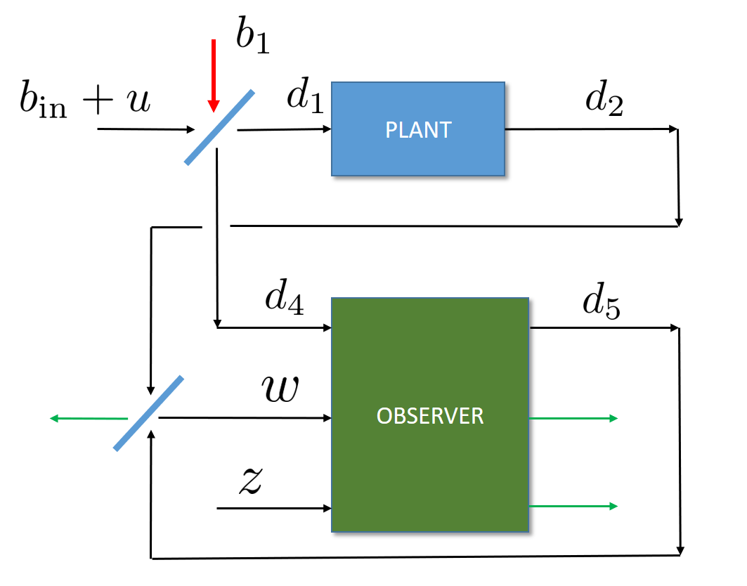
We first set about replacing junctions $J_{1}$ and $J_{4}$ with beam-splitters. To keep things simple, we ignore junctions $J_{2}$ and $J_{3}$ though this means that we cannot now pass the relevant outputs of the plant and observer to the outside world as before. The situation is depicted in Figure 4. Note that we need to introduce a new independent quantum input process $b_{1}$ (highlighted in red). The plant will be a cavity mode $a$ with frequency $\omega$ and a single input leading to a damping rate $\gamma$, (so $A=-\frac{1}{2}\gamma-i\omega,B=-\sqrt{\gamma},C=\sqrt{\gamma}$).

For the observer, we need a minimum of two inputs $b_{\text{in},1}\equiv d_{4}$ and $b_{\text{in},2}\equiv w$, see Figure 4, with coupling operators $L_{1}=\sqrt{\gamma}\tilde{a}$ and $L_{2}=\sqrt{\gamma_{L}}\tilde{a}$. Here $L=\sqrt{\gamma_{L}}$ is the quantum Luenberger gain coefficient. However, on its own, this would lead to $A^{\text{obs}}=-\frac{1}{2}(\gamma+\gamma_{L})-i\omega$ so we have introduced more damping into the observer than in the plant leading to a different $A$ matrix. The choice of $L_{1}$ is constrained to ensure that the $B$ and $C$ coefficients of the plant and observer match up, so we cannot adjust this.

Figure 4: (color online) A quantum plant and observer

The only other option is to introduce a third input $b_{\text{in},3}$ whose role is to supply energy to compensate for $b_{\text{in},2}$: this is achieved by taking the associate coupling to be $L_{3}=\sqrt{\gamma_{L}}\tilde{a}^{\ast}$. The observer is then described by

$$\frac{d}{dt}\tilde{a}\left(t\right) = -\left(\frac{1}{2}\gamma+i\omega\right)\tilde{a}\left(t\right)-\sqrt{\gamma}b_{\text{in},1}\left(t\right)$$ (12)

$$-\sqrt{\gamma_{L}}b_{\text{in},2}\left(t\right)-\sqrt{\gamma_{L}}b_{\text{in},3}\left(t\right)^{\ast}$$

with $b_{\text{out},1}\left(t\right)=\sqrt{\gamma}\tilde{a}\left(t\right)+b_{\text{in},1}\left(t\right)$, $b_{\text{out},2}\left(t\right)=\sqrt{\gamma_{L}}\tilde{a}\left(t\right)+b_{\text{in},2}\left(t\right)$, $b_{\text{out},3}\left(t\right)=\sqrt{\gamma_{L}}\tilde{a}\left(t\right)^{\ast}+b_{\text{in},3}\left(t\right)$.

The outputs $b_{\text{out},2}\left(t\right)$ and $b_{\text{out},3}\left(t\right)$ are ignored, however, we see comparing (8) and (12) that the $A$ coefficients are equal, as are the $B$ and $C$ coefficients or $b_{\text{in}}\left(t\right)$ and $b_{\text{in},1}\left(t\right)$.

The relevant equations, with reference to Figure 4, are

$$(J_{1}\,\text{Beam-splitter})\qquad\left\{\begin{array}[]{c}d_{1}=\frac{1}{\sqrt{2}}(b_{\text{in}}+u)+\frac{1}{\sqrt{2}}b_{1},\\ d_{4}=\frac{1}{\sqrt{2}}(b_{\text{in}}+u)-\frac{1}{\sqrt{2}}b_{1};\end{array}\right.$$

$$(J_{4}\,\text{Beam-splitter})\qquad w=\frac{1}{\sqrt{2}}d_{2}-\frac{1}{\sqrt{2}}d_{5};$$

$$(\text{Plant})\quad\left\{\begin{array}[]{c}\dot{a}=Aa+Bd_{1}\\ d_{2}=Ca+d_{1};\end{array}\right.$$

$$(\text{Observer})\quad\left\{\begin{array}[]{c}\dot{a}=A\tilde{a}+Bd_{4}-Lw,\\ d_{5}=C\tilde{a}+d_{4}.\end{array}\right.$$

We now introduce the error operator defined to be $e=a-\tilde{a}$ and after some algebra we find $\dot{e}=\big{(}A-\frac{1}{\sqrt{2}}LC\big{)}e\left(t\right)-\sqrt{2}\left(C+L\right)b_{1}\left(t\right)$, or

$$\dot{e}\equiv\left(-\frac{1}{2}\gamma-\sqrt{\frac{\gamma\gamma_{L}}{2}}+i\omega\right)e\left(t\right)-\sqrt{2}\left(\sqrt{\gamma}+\sqrt{\gamma_{L}}\right)b_{1}\left(t\right).$$

III.2 Verifiable Quantum Luenberger Observers

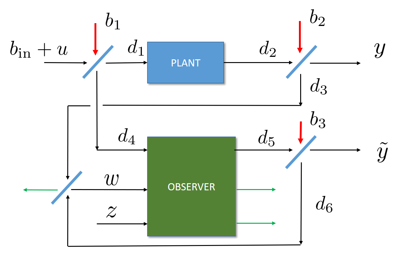
If we wish to verify the convergence then we may consider the setup in Figure 5. This time, $\dot{e}(t)=\big{(}A-\frac{1}{\sqrt{2}}LC\big{)}e\left(t\right)-\sqrt{2}\left(C+\frac{1}{2}L\right)b_{1}(t)-\frac{1}{2}Lb_{2}(t)+\frac{1}{2}Lb_{3}(t)-Lz^{\ast}(t)$.

Figure 5: (color online) Verifiable quantum observer

We may send the outputs $y$ and $\tilde{y}$ into a 50-50 beam-splitter and measure the output

$$\frac{y(t)-\tilde{y}(t)}{\sqrt{2}}=\frac{1}{\sqrt{2}}C\,e(t)+b_{1}(t)+\frac{1}{\sqrt{2}}b_{2}(t)-\frac{1}{\sqrt{2}}b_{3}(t).$$

Note that this output is likewise unaffected by any input disturbance $u$ and on average decays to zero as $\langle e(t)\rangle\to 0$ for large time.

IV Conclusion

We have given an explicit construction for a coherent quantum observer which observes a quantum system without altering its dynamics. In common with the classical Luenberger observer, any disturbance $u$ carried into the plant system does not get transferred to the observer. All inputs act passively on the cavity modes, except the input $z$ which supplies an active element in the observer to compensate the additional damping and ensure that the appropriate observer $A-B-C$ terms agree with those of the plant system.

The observer may be physically realized, however it is also of conceptual value in observer-based design of quantum coherent feedback controllers.

References

• (1) D.G. Luenberger. IEEE Transactions on Military Electronics, 8(2):74-80, 1964.
• (2) D.G. Luenberger. IEEE Transactions on Automatic Control, 11(2):190-199, 1966.
• (3) R. van Handel, L. Bouten, In Quantum Stochastics and Information: Statistics, Filtering and Control (V. P. Belavkin and M. I. Guta, eds.), World Scientific, 2008.
• (4) Z. Miao and M. R. James. In Proceedings of 51st IEEE Conference on Decision and Control, pages 1680-1684, Maui, Hawaii, 2012.
• (5) Z. Miao, M. R. James, and V. Ugrinovskii. arXiv: 1509.05124, 2015.
• (6) Z. Miao, M.R. Hush, and M.R. James. Phys. Rev. A, 92(1):012115, 2015.
• (7) Y. Pan, T. Nguyen, Z. Miao, N. Amini, V.Ugrinovski, and M.R. James. In Proceedings of the 35th Chinese Control Conference July 27-29, 2016, Chengdu, China
• (8) R.L. Hudson and K.R. Parthasarathy, Commun. Math. Phys., vol. 93, pp. 301-323, 1984.
• (9) C.W. Gardiner and P. Zoller. Quantum Noise. Springer Series in Synergetics. Springer, New York, 2nd edition, 2000.
• (10) H.I. Nurdin, J.E. Gough. Quantum Inf. Comput. 15, pp 1017-1040, 2015.