Partial Least Squares Regression on Riemannian Manifolds
and Its Application in Classifications

Abstract

Partial least squares regression (PLSR) has been a popular technique to explore the linear relationship between two datasets. However, most of algorithm implementations of PLSR may only achieve a suboptimal solution through an optimization on the Euclidean space. In this paper, we propose several novel PLSR models on Riemannian manifolds and develop optimization algorithms based on Riemannian geometry of manifolds. This algorithm can calculate all the factors of PLSR globally to avoid suboptimal solutions. In a number of experiments, we have demonstrated the benefits of applying the proposed model and algorithm to a variety of learning tasks in pattern recognition and object classification.

1 Introduction

Partial least squares regression (PLSR) is a statistical method for modeling a linear relationship between two data sets, which may be two different descriptions of an object. Instead of finding hyperplanes of maximum variance of the original datasets, it finds the maximum degree of linear association between two latent components which are the projection of two original data sets to a new space, and based on those latent components, regresses the loading matrices of the two original datasets, respectively. Compared with the multiple linear regression (MLR)(?) and principal component regression (PCR) (?; ?), PLSR has also been proved to be not only useful for high-dimensional data (?; ?), but also to be a good alternative because it is more robust and adaptable (?). Robust means that the model parameters do not change very much when new training samples are taken from the same total population. Thus PLSR has wide applications in several areas of scientific research (?; ?; ?; ?; ?) since the 1960s.

There exist many forms of PLSR, such as NIPALS (the nonlinear iterative partial least squares)(?), PLS1 (one of the data sets consists of a single variable)(?) and PLS2 (both data sets are multidimensional) where a linear inner relation between the projection vectors exists, PLS-SB (?; ?), where the extracted projection matrices are in general not mutually orthogonal, statistically inspired modification of PLS (SIMPLS) (?), which calculates the PLSR factors directly as linear combinations of the original data sets, Kernel PLSR (?) applied in a reproducing kernel Hilbert space, and Sparse PLSR (?) to achieve factors selection by producing sparse linear combinations of the original data sets.

However, it is difficult to directly solve for projection matrices with orthogonality as a whole in Euclidean spaces. To the best of our knowledge, all the existing algorithms greedily proceed through a sequence of low-dimensional subspaces: the first dimension is chosen to optimize the PLSR objective, e.g., maximizing the covariance between the projected data sets, and then subsequent dimensions are chosen to optimize the objective on a residual or reduced data sets. In some sense, this can be actually fruitful but limited, often resulting in ad hoc or suboptimal solutions. To overcome the shortcoming, we are devoted to proposing several novel models and algorithms to solve PLSR problems under the framework of Riemannian manifold optimisation (?). For the optimisation problems from PLSR, the orthogonality constraint can be easily eliminated in Stiefel/Grassmann manifolds with the possibility of solving the factors of PLSR as a whole and being steadily convergent at global optimum.

In general, Riemannian optimization is directly based on the curved manifold geometry such as Stiefel/Grassmann manifolds, benefiting from a lower complexity and better numerical properties. The geometrical framework of Stiefel and Grassmann manifolds were proposed in (?). Stiefel manifold was successfully applied in neural networks (?) and linear dimensionality reduction (?). Meanwhile, Grassmann manifold has been studied in two major fields, data analysis such as video stream analysis (?), clustering subspaces into classes of subspaces (?; ?), and parameter analysis such as an unifying view on the subspace-based learning method (?), and optimization over the Grassmann manifold (?; ?). According to (?; ?), the generalized Stiefel manifold is endowed with a scaled metric by making it a Riemannian submanifold based on Stiefel manifold, which is more flexible to the constraints of the optimization raised from the generalised PLSR. Generalized Grassmann manifold is generated by the Generalized Stiefel manifold, and each point on this manifold is a collection of “scaled” vector subspaces of dimension $p$ embedded in $\mathbb{R}^{n}$. Another important matrix manifold is the oblique manifold which is a product of spheres. Absil et al. (?) investigate the geometry of this manifold and show how independent component analysis can be cast on this manifold as non-orthogonal joint diagonalization.

Some conceptual algorithms and its convergence analysis based on ideas of Riemannian manifolds, and the efficient numerical implementation (?) have been developed recently. This has paved the way for one to investigate overall algorithms to solve PLSR problems based on optimization algorithms on Riemannian manifolds. Particularly, Mishra et al. (?) have developed a useful MATLAB toolbox ManOpt (Manifold Optimization) http://www.manopt.org/ which can be perfectly adopted in this research to test the algorithms to be developed.

The contributions of this paper are:

1. We establish several novel PLSR models on Riemannian manifolds and give some matrices representations of relate optimization ingredients;

2. We give new algorithms for the proposed PLSR model on Riemannian manifolds, which are able to calculate all the factors as a whole so as to obtain optimal solutions.

2 Notations and Preliminaries

This section will briefly describe some notations and concepts that will be used throughout the paper.

2.1 Notations

We denote matrices by boldface capital letters, e.g., $\mathbf{A}$, vectors by boldface lowercase letters, e.g., $\mathbf{a}$, and scalars by letters, e.g., $a$. The superscript $T$ denotes the transpose of a vector/matrix. $\text{diag}(\mathbf{A})$ denotes the diagonal matrix with elements from the diagonal of $\mathbf{A}$. $\mathbf{B}\succ 0$ means that $\mathbf{B}$ is a positive definite matrix. The SVD decomposition of a matrix $\mathbf{A}\in\mathbb{R}^{m\times n}$ is denoted by $\mathbf{A}=\mathbf{U}\boldsymbol{\Sigma}\mathbf{V}^{T}$, while the eigendecomposition of a diagonable square matrix $\mathbf{A}\in\mathbb{R}^{n\times n}$ is denoted by $\mathbf{A}=\mathbf{E}_{v}\mathbf{E}_{\lambda}\mathbf{E}_{v}^{-1}$.

The set of all $c$-order orthogonal matrices is denoted by

$$\mathcal{O}(c)=\{\mathbf{U}\in\mathbb{R}^{c\times c}|\mathbf{U}^{T}\mathbf{U}=\mathbf{U}\mathbf{U}^{T}=\mathbf{I}_{c}\},$$

also called orthogonal group of order $c$. The Stiefel manifold is the set of all the matrices whose columns are orthogonal, denoted by

$$St(p,c)=\{\mathbf{W}\in\mathbb{R}^{p\times c}|\mathbf{W}^{T}\mathbf{W}=\mathbf{I}_{c}\}.$$ (1)

Given a Stiefel manifold $St(p,c)$, the related Grassmann manifold $Gr(p,c)$ can be formed as the quotient space of $St(p,c)$ under the equivalent relation defined by the orthogonal group $\mathcal{O}(c)$, i.e.

$$G(p,c)=St(p,c)/\mathcal{O}(c).$$ (2)

Two Stiefel points $\mathbf{W}_{1},\mathbf{W}_{2}\in St(p,c)$ are equivalent to each other, if there exists an $\mathbf{O}\in\mathcal{O}(c)$ such that $\mathbf{W}_{1}=\mathbf{W}_{2}\mathbf{O}$. We use $[\mathbf{W}]\in Gr(p,c)$ to denote the equivalent class for a given $\mathbf{W}\in St(p.c)$, and $\mathbf{W}$ is called a representation of the Grassmann point $[\mathbf{W}]$. More intuitively, Grassmann manifold is the set of all $c$-dimensional subspaces in $\mathbb{R}^{p}$.

In this paper, we are also interested in the so-called generalized Stiefel manifold which is defined under the $\mathbf{B}$-orthogonality

$$GSt(p,c;\mathbf{B})=\{\mathbf{W}\in\mathbb{R}^{p\times c}|\mathbf{W}^{T}\mathbf{B}\mathbf{W}=\mathbf{I}_{p}\},$$ (3)

where $\mathbf{B}\in\mathbb{R}^{c\times c}$ is a given positive definite matrix. And similarly the generalized Grassmann manifold is defined by

$$GGr(p,c;\mathbf{B})=GSt(p,c;\mathbf{B})/\mathcal{O}(c).$$ (4)

If we relax the orthogonal constraints but retain unit constraint, we have the so-called Oblique manifold which consists of all the $p\times c$ matrices whose columns are unit vectors. That is

$$Ob(p,c)=\{\mathbf{W}\in\mathbb{R}^{p\times c},\text{diag}(\mathbf{W}^{T}\mathbf{W})=\mathbf{I}_{c}\}.$$ (5)

2.2 Partial Least Squares Regression (PLSR)

Let $\mathbf{x}_{i}=[x_{i1},x_{i2},\ldots,x_{ip}]^{T}\in\mathbb{R}^{p}$, $(i=1,2,\ldots,n)$ are $n$ observation samples and $\mathbf{y}_{i}=[y_{i1},y_{i2},\ldots,y_{iq}]^{T}\in\mathbb{R}^{q}$, $(i=1,2,\ldots,n)$ are $n$ response data. Then $\mathbf{X}=[\mathbf{x}_{1},\mathbf{x}_{2},...,\mathbf{x}_{n}]^{T}\in\mathbb{R}^{n\times p}$, $\mathbf{Y}=[\mathbf{y}_{1},\mathbf{y}_{2},...,\mathbf{y}_{n}]^{T}\in\mathbb{R}^{n\times q}$.

Suppose there exists a linear regression relation

$$\mathbf{Y}=\mathbf{X}\mathbf{R}+\mathbf{E},$$ (6)

where $\mathbf{R}$ is the regression coefficient and $\mathbf{E}$ is the residual matrix. PLSR is usually an effective approach to dealing with the case of $n<p$ when the classical linear regression fails since the $p\times p$ covariance matrix $\mathbf{X}^{T}\mathbf{X}$ is singular.

In order to obtain $\mathbf{R}$, PLSR generally decomposes datasets $\mathbf{X}$ and $\mathbf{Y}$ ($\mathbf{X}$ and $\mathbf{Y}$ are preprocessed to be zero-mean data) into the following form

$$\begin{split}&\mathbf{X}_{n\times p}=\mathbf{t}_{n\times 1}\mathbf{p}_{p\times 1}^{T}+\mathbf{E}_{n\times p}\\ &\mathbf{Y}_{n\times q}=\mathbf{u}_{n\times 1}\mathbf{q}_{q\times 1}^{T}+\mathbf{F}_{n\times q}\end{split}$$ (7)

where $\mathbf{t}$ and $\mathbf{u}$ are vectors giving the latent components for the $n$ observations, $\mathbf{p}$ and $\mathbf{q}$ represent loading vectors. $\mathbf{E}$ and $\mathbf{F}$ are residual matrices.

PLSR searches the latent components $\mathbf{t}=\mathbf{X}\mathbf{w}$ and $\mathbf{u}=\mathbf{Y}\mathbf{g}$ such that the squared covariance between them is maximized, where the projection vectors $\mathbf{w}$ and $\mathbf{g}$ satisfy the constraints $\mathbf{w}^{T}\mathbf{w}=1$ and $\mathbf{g}^{T}\mathbf{g}=1$, respectively. The solution is given by

$$\begin{split}\max_{\|\mathbf{w}\|=\|\mathbf{g}\|=1}[\text{cov}(\mathbf{t},\mathbf{u})]^{2}&=\max_{\|\mathbf{w}\|=\|\mathbf{g}\|=1}(\mathbf{w}^{T}\mathbf{X}^{T}\mathbf{Y}\mathbf{g})^{2}.\end{split}$$ (8)

It can be shown that the projection vector $\mathbf{w}$ corresponds to the first eigenvector of $\mathbf{X}^{T}\mathbf{Y}\mathbf{Y}^{T}\mathbf{X}$ (?; ?) and the optimal solution $\mathbf{w}$ of

$$\max_{\|\mathbf{w}\|=1}\mathbf{w}^{T}\mathbf{X}^{T}\mathbf{Y}\mathbf{Y}^{T}\mathbf{X}\mathbf{w}$$ (9)

is also the first eigenvector of $\mathbf{X}^{T}\mathbf{Y}\mathbf{Y}^{T}\mathbf{X}$. Thus both objectives (8) and (9) have the same solution on $\mathbf{w}$.

We can also obtain $\mathbf{g}$ while swapping the position of $\mathbf{X}$ and $\mathbf{Y}$. After obtaining the projection vectors $\mathbf{w}$ and $\mathbf{g}$, the latent vectors $\mathbf{t}=\mathbf{X}\mathbf{w}$ and $\mathbf{u}=\mathbf{Y}\mathbf{g}$ are also acquired.

The essence of (8) is to maximum degree of linear association between $\mathbf{t}$ and $\mathbf{u}$. Suppose that a linear relation between the latent vectors $\mathbf{t}$ and $\mathbf{u}$ exists, e.i. $\mathbf{u}=\mathbf{t}d+\mathbf{h}$ , where $d$ is a constant, $\mathbf{h}$ is error term, and $d$ and $\mathbf{h}$ can be absorbed by $\mathbf{q}$ and $\mathbf{F}$, respectively. Based on this relation, (7) can be casted as the following formula

$$\mathbf{X}=\mathbf{t}\mathbf{p}^{T}+\mathbf{E},\ \ \mathbf{Y}=\mathbf{t}\mathbf{q}^{T}+\mathbf{F}$$ (10)

Thus $\mathbf{p}=\mathbf{X}^{T}\mathbf{t}(\mathbf{t}^{T}\mathbf{t})^{-1}$ and $\mathbf{q}=\mathbf{Y}^{T}\mathbf{t}(\mathbf{t}^{T}\mathbf{t})^{-1}$ can be obtained by the least square method. Then $\mathbf{X}$ and $\mathbf{Y}$ can be updated

$$\mathbf{X}:=\mathbf{X}-\mathbf{t}\mathbf{p}^{T},\ \ \mathbf{Y}:=\mathbf{Y}-\mathbf{t}\mathbf{q}^{T}$$ (11)

This procedure is re-iterated $c$ times, and we can obtain the projection matrix $\mathbf{W}=[\mathbf{w}_{1},\mathbf{w}_{2},\ldots,\mathbf{w}_{c}]$, latent components $\mathbf{T}=[\mathbf{t}_{1},\mathbf{t}_{2},\ldots,\mathbf{t}_{c}]$, loading matrices $\mathbf{P}=[\mathbf{p}_{1},\mathbf{p}_{2},\ldots,\mathbf{p}_{c}]$ and $\mathbf{Q}=[\mathbf{q}_{1},\mathbf{q}_{2},\ldots,\mathbf{q}_{c}]$. And (10) can be recast as

$$\mathbf{X}=\mathbf{T}\mathbf{P}^{T}+\mathbf{E},\ \ \mathbf{Y}=\mathbf{T}\mathbf{Q}^{T}+\mathbf{F}$$ (12)

According to $\mathbf{T}=\mathbf{X}\mathbf{W}$, $\mathbf{Y}=\mathbf{X}\mathbf{W}\mathbf{Q}^{T}+\mathbf{F}$ and regression coefficient $\mathbf{R}=\mathbf{W}\mathbf{Q}^{T}$.

3 The PLSR on Riemannian Manifolds

The core of PLSR is to optimize the squared covariance between latent components $\mathbf{T}$ and the data $\mathbf{Y}$, see (9). Boulesterx and Strimmer (?) had summarized several different model modification for optimizing the projection matrix $\mathbf{W}$ in Euclidean spaces. However all the algorithms take a greedy strategy to calculate all the factors one by one, and thus often result in suboptimal solutions. In order to overcome this shortcoming, this paper will take those models as optimization on Riemannian manifolds, and propose an algorithms for solving the projection matrix $\mathbf{W}$ thus the latent component matrix $\mathbf{T}$ as a whole on Riemannian manifolds.

3.1 SIMPLSR on the Generalized Grassmann Manifolds

We can transform model (9) into following optimization problem

$$\max_{\mathbf{W}}\text{tr}(\mathbf{W}^{T}\mathbf{X}^{T}\mathbf{Y}\mathbf{Y}^{T}\mathbf{X}\mathbf{W})\ \ \text{s.t.}\ \ \mathbf{W}^{T}\mathbf{W}=\mathbf{I}$$ (13)

where $\mathbf{W}\in\mathbb{R}^{p\times c}$ and $\mathbf{I}$ is the identity matrix.

Because of the orthogonal constraint, this constrained optimization problem can be taken as unconstrained optimization on Stiefel manifold

$$\max_{\mathbf{W}\in St(p,c)}\text{tr}(\mathbf{W}^{T}\mathbf{X}^{T}\mathbf{Y}\mathbf{Y}^{T}\mathbf{X}\mathbf{W}).$$ (14)

Algorithm 1 SIMPLSR on generalized Grassmann manifold (PLSRGGr)

0:  matrices $\mathbf{X}\in\mathbb{R}^{n\times p},\mathbf{Y}\in\mathbb{R}^{n\times q}$.

1:  Initial matrix $\mathbf{W}_{1}$ is a randomly generated matrix, gradient norm tolerance $\epsilon_{1}$, step size tolerance $\epsilon_{2}$ and max iteration number $N$. Let $0<c<1$ $\beta_{1}$ =0 and $\boldsymbol{\zeta}_{0}=\mathbf{0}$.

2:  for $k=1:N$ do

3:     Compute gradient in Euclidean space

$$\text{grad}_{E}f(\mathbf{W}_{k})=2\mathbf{X}^{T}\mathbf{Y}\mathbf{Y}^{T}\mathbf{X}\mathbf{W}_{k}$$

4:     Compute gradient on generalized Grassmann manifold

$$\boldsymbol{\eta}_{k}=\mathcal{P}_{[\mathbf{W}_{k}]}(\text{grad}_{E}f(\mathbf{W}_{k})),$$

where Projection operator

$$\mathcal{P}_{\mathbf{W}_{k}}(\mathbf{Z})=\mathbf{Z}-\mathbf{W}_{k}\text{symm}(\mathbf{W}_{k}^{T}\mathbf{X}^{T}\mathbf{X}\mathbf{Z}),$$

$$\text{symm}(\mathbf{D})=(\mathbf{D}+\mathbf{D}^{T})/2.$$

5:     if $k\geq 2$ then

6:        Compute the weighted value

$$\beta_{k}=\text{tr}(\boldsymbol{\eta}_{k}^{T}\boldsymbol{\eta}_{k})/\text{tr}(\boldsymbol{\eta}_{k-1}^{T}\boldsymbol{\eta}_{k-1})$$

7:        Compute a transport direction

$$\mathcal{T}_{\mathbf{W}_{k-1}\rightarrow\mathbf{W}_{k}}(\boldsymbol{\zeta_{k-1}})=\mathcal{P}_{\mathbf{W}_{k}}(\boldsymbol{\zeta_{k-1}}).$$

8:     end if

9:     Compute a conjugate direction

$$\boldsymbol{\zeta}_{k}=-\text{grad}_{R}f(\mathbf{W}_{k})+\beta_{k}\mathcal{T}_{\mathbf{W}_{k-1}\rightarrow\mathbf{W}_{k}}(\boldsymbol{\zeta_{k-1}}).$$

10:     Choose a step size $\alpha_{k}$ satisfying the Armijo criterion

$$f(R_{\mathbf{W}_{k}}(\alpha_{k}\boldsymbol{\zeta}_{k})\geq f(\mathbf{W}_{k})+c\alpha_{k}\text{tr}(\boldsymbol{\eta}_{k}^{T}\boldsymbol{\zeta}_{k}),$$

where Retraction operator

$$\mathcal{R}_{[\mathbf{W}_{k}]}(\boldsymbol{\zeta}_{k})=\mathbf{U}\mathbf{E}s\mathbf{E}v^{T}\mathbf{V}^{T};$$

$\mathbf{W}_{k}+\boldsymbol{\zeta}_{k}=\mathbf{U}\boldsymbol{\Sigma}\mathbf{V},$ (SVD decomposition) $\mathbf{U}^{T}\mathbf{X}^{T}\mathbf{X}\mathbf{U}=\mathbf{E}v\mathbf{E}_{\lambda}\mathbf{E}v^{-1}$ (eigendecomposition), $\mathbf{E}s=\mathbf{E}v(\mathbf{E}_{\lambda})^{-1/2}$. Set $\mathbf{W}_{k+1}=R_{\mathbf{W}_{k}}(\alpha_{k}\boldsymbol{\zeta}_{k})$.

11:     Terminate and output $\mathbf{W}_{k+1}$ if one of the stopping conditions is satisfied $\|\boldsymbol{\eta}_{k+1}\|_{F}\leq\epsilon_{1}$, $\alpha_{k}\leq\epsilon_{2}$ and $k\geq N$ is achieved.

12:  end for

13:  $\mathbf{W}=\mathbf{W}_{k+1}$.

14:  Compute $\mathbf{T}=\mathbf{X}\mathbf{W}$.

15:  Compute $\mathbf{P}=\mathbf{X}^{T}\mathbf{T}(\mathbf{T}^{T}\mathbf{T})^{-1}$.

16:  Compute $\mathbf{Q}=\mathbf{Y}^{T}\mathbf{T}(\mathbf{T}^{T}\mathbf{T})^{-1}$.

17:  Compute regression coefficient $\mathbf{R}=\mathbf{W}\mathbf{Q}^{T}$.

17:  $\mathbf{W,T,P,Q,R}$.

To represent the data sets $\mathbf{X}$ and $\mathbf{Y}$ from (12), it is more reasonable to constrain latent components $\mathbf{T}$ in an orthogonal space. Thus model (14) can be rewritten as

$$\begin{split}&\max_{\mathbf{W}}\text{tr}(\mathbf{W}^{T}\mathbf{X}^{T}\mathbf{Y}\mathbf{Y}^{T}\mathbf{X}\mathbf{W}),\\ &\text{s.t.}\mathbf{T}^{T}\mathbf{T}=\mathbf{W}^{T}\mathbf{X}^{T}\mathbf{X}\mathbf{W}=\mathbf{I}.\end{split}$$ (15)

Similar to model (13), we can first convert problem (15) to an unconstrained problem on the generalized Stiefel manifold with $\mathbf{B}=\mathbf{X}^{T}\mathbf{X}$, i.e.,

$$\max_{\mathbf{W}\in GSt(p,c,\mathbf{X}^{T}\mathbf{X})}\text{tr}(\mathbf{W}^{T}\mathbf{X}^{T}\mathbf{Y}\mathbf{Y}^{T}\mathbf{X}\mathbf{W}).$$ (16)

Let $f(\mathbf{W})=\text{tr}(\mathbf{W}^{T}\mathbf{X}^{T}\mathbf{Y}\mathbf{Y}^{T}\mathbf{X}\mathbf{W})$ be defined on generalized Stiefel manifold $GSt(p,c,\mathbf{B})$. For any matrix $\mathbf{U}\in\mathcal{O}(c)$, we have $f(\mathbf{W}\mathbf{U})=f(\mathbf{W})$. This means that the maximizer of $f$ is unidentifiable on generalized Stiefel in the sense that if $\mathbf{W}$ is a solution to (16), then so is $\mathbf{W}\mathbf{U}$ for any $\mathbf{U}\in\mathcal{O}(c)$. This may cause some trouble for numerical algorithms for solving (16).

If we contract all the generalized Stiefel points in its equivalent class $[\mathbf{W}]=\{\mathbf{W}\mathbf{U}|\text{ for all }\mathbf{U}\in\mathcal{O}(c)\}$ together, it is straightforward to convert the optimization (16) on generalized Stiefel manifold to the generalized Grassmann manifold $GGr(p,c,\mathbf{B})$ (?) as follows

$$\max_{[\mathbf{W}]\in GGr(p,c)}\text{tr}(\mathbf{W}^{T}\mathbf{X}^{T}\mathbf{Y}\mathbf{Y}^{T}\mathbf{X}\mathbf{W}),$$ (17)

The model (17) is called as statistically inspired modification of PLSR (SIMPLSR) on generalized Grassmann manifolds.

We will use the metric $g_{[\mathbf{W}]}(\mathbf{Z}_{1},\mathbf{Z}_{2})=\text{tr}(\mathbf{Z}_{1}^{T}\mathbf{B}\mathbf{Z}_{2})$ on generalized Grassmann manifold. The matrix representation of the tangent space of the generalized Grassmann manifold is identified with a subspace of the tangent space of the total space that does not produce a displacement along the equivalence classes. This subspace is called the horizontal space (?). The horizontal space $\mathcal{H}_{[\mathbf{W}]}GGr(p,c)=\{\mathbf{Z}\in\mathbb{R}^{p\times c}:\mathbf{W}^{T}\mathbf{Z}=0\}$. The other related ingredients such as projection operator, retraction operator, transport operator for implementing an off-the-shelf nonlinear conjugate-gradient algorithm (?) for (17) are listed in Algorithm 1 which is the optimization algorithm of PLSR on generalized Grassmann manifold.

3.2 SIMPLSR on Product Manifolds

Another equivalent expression for SIMPLSR (?) which often appear in the literature is as follows

$$\max_{(\mathbf{W},\mathbf{U})}\text{tr}(\mathbf{W}^{T}\mathbf{X}^{T}\mathbf{Y}\mathbf{U}),$$ (18)

$$\text{s.t.}\ \ \mathbf{T}^{T}\mathbf{T}=\mathbf{W}^{T}\mathbf{X}^{T}\mathbf{X}\mathbf{W}=\mathbf{I}\ \text{and}\ \ \text{diag}(\mathbf{U}^{T}\mathbf{U})=\mathbf{I}.$$

The feasible domain of $\mathbf{W}$ and $\mathbf{U}$ can be considered as a product manifold of a generalized Stiefel manifold $GSt(p,c,\mathbf{B})$ with $\mathbf{B}=\mathbf{X}^{T}\mathbf{X}$ (see (3)) and Oblique manifold $Ob(q,c)$ (see (5)), respectively. The product manifold is denoted as

$$\begin{split}&GSt(p,c,\mathbf{B})\times Ob(q,c)\\ =&\{(\mathbf{W},\mathbf{U}):\mathbf{W}\in GSt(p,c,\mathbf{B}),\mathbf{U}\in Ob(q,c)\}.\end{split}$$ (19)

Algorithm 2 SIMPLSR on product manifold (PLSRGStO)

0:  matrices $\mathbf{X}\in\mathbb{R}^{n\times p},\mathbf{Y}\in\mathbb{R}^{n\times q}$.

1:  Initial matrices $\mathbf{W}_{1}$ and $\mathbf{U}_{1}$ are randomly generated matrices, gradient norm tolerance $\epsilon_{1}$, step size tolerance $\epsilon_{2}$ and max alternating iterations $N_{1}$, max iteration number $N_{2}$. . Let $0<c<1$ $\beta_{1}$ =0 and $\boldsymbol{\zeta}_{0}=\mathbf{0}$.

2:  for $k=1:N_{1}$ do

3:     for $i=1:N_{2}$ do

4:        Compute gradient in Euclidean space$\text{grad}_{E}f_{\mathbf{W}}(\mathbf{W}_{i})=\mathbf{X}^{T}\mathbf{Y}\mathbf{U}_{1}$

5:        Some related ingredients of generalized Stiefel manifold are same with generalized Grassmann manifold, and $\mathbf{W}$ can be solved by Algorithm 1.

6:     end for

7:     $\mathbf{W}_{1}=\mathbf{W}_{i}$.

8:     for $j=1:N_{2}$ do

9:        Compute gradient in Euclidean space

$$\text{grad}_{E}f_{\mathbf{U}}(\mathbf{U}_{j})=\mathbf{Y}^{T}\mathbf{X}\mathbf{W}_{1}$$

10:        Compute gradient on Oblique manifold

$$\boldsymbol{\eta}_{j}=\mathcal{P}_{\mathbf{U}_{j}}(\text{grad}_{E}f(\mathbf{U}_{j})),$$

where Projection operator

$$\mathcal{P}_{\mathbf{U}_{j}}(\mathbf{Z})=\mathbf{Z}-\mathbf{U}_{j}\text{diag}(\mathbf{U}_{j}^{T}\mathbf{Z})$$

.

11:        if $j\geq 2$ then

12:           Compute the weighted value

$$\beta_{j}=\text{tr}(\boldsymbol{\eta}_{j}^{T}\boldsymbol{\eta}_{j})/\text{tr}(\boldsymbol{\eta}_{j-1}^{T}\boldsymbol{\eta}_{j-1})$$

13:           Compute a transport direction

$$\mathcal{T}_{\mathbf{U}_{j-1}\rightarrow\mathbf{U}_{j}}(\boldsymbol{\zeta_{j-1}})=\mathcal{P}_{\mathbf{U}_{j}}(\boldsymbol{\zeta_{j-1}}).$$

14:           Compute a conjugate direction

$$\boldsymbol{\zeta}_{j}=-\boldsymbol{\eta}_{j}+\beta_{j}\mathcal{T}_{\mathbf{U}_{j-1}\rightarrow\mathbf{U}_{j}}(\boldsymbol{\zeta_{j-1}}).$$

15:        end if

16:        Choose a step size $\alpha_{j}$ satisfying the Armijo criterion

$$f(R_{\mathbf{U}_{j}}(\alpha_{j}\boldsymbol{\zeta}_{j})\geq f(\mathbf{U}_{j})+c\alpha_{j}\text{tr}(\boldsymbol{\eta}_{j}^{T}\boldsymbol{\zeta}_{j}).$$

where Retraction operator $\mathcal{R}_{\mathbf{U}_{j}}(\boldsymbol{\zeta}_{j})=(\mathbf{U}_{j}+\boldsymbol{\zeta}_{j})(\text{diag}((\mathbf{U}_{j}+\boldsymbol{\zeta}_{j})^{T}(\mathbf{U}_{j}+\boldsymbol{\zeta}_{j})))^{-1/2}.$

17:        Terminate and output $\mathbf{U}_{j+1}$ if one of the stopping conditions is satisfied $\|\boldsymbol{\eta}_{j+1}\|_{F}\leq\epsilon_{1}$, $\alpha_{j}\leq\epsilon_{2}$ and $j\geq N_{2}$ is achieved.

18:     end for

19:     $\mathbf{U}_{1}=U_{j+1}$

20:  end for

21:  Compute $\mathbf{T}=\mathbf{X}\mathbf{W}_{1}$.

22:  Compute $\mathbf{P}=\mathbf{X}^{T}\mathbf{T}(\mathbf{T}^{T}\mathbf{T})^{-1}$.

23:  Compute $\mathbf{Q}=\mathbf{Y}^{T}\mathbf{T}(\mathbf{T}^{T}\mathbf{T})^{-1}$.

24:  Compute regression coefficient $\mathbf{R}=\mathbf{W}\mathbf{Q}^{T}$.

24:  $\mathbf{W,T,P,Q,R}$.

So model (18) can be modified as

$$\max_{(\mathbf{W},\mathbf{U})\in St(p,c,\mathbf{B})\times Ob(q,c)}\text{tr}(\mathbf{W}^{T}\mathbf{X}^{T}\mathbf{Y}\mathbf{U})$$ (20)

We call this model as equivalent statistically inspired modification of PLSR (ESIMPLSR) on product manifolds.

To induce the geometry of the product manifold, we use the metric $g_{\mathbf{W}}(\mathbf{Z}_{1},\mathbf{Z}_{2})=\text{tr}(\mathbf{Z}_{1}^{T}\mathbf{B}\mathbf{Z}_{2})$ and the tangent space $T_{\mathbf{W}}GSt(p,c,\mathbf{B})=\{\mathbf{Z}\in\mathbb{R}^{p\times c}:\mathbf{W}^{T}\mathbf{B}\mathbf{Z}+\mathbf{Z}^{T}\mathbf{B}\mathbf{W}=\mathbf{0}\}$ on the generalized Stiefel manifold, and the metric $g_{\mathbf{U}}(\mathbf{Z}_{1},\mathbf{Z}_{2})=\text{tr}(\mathbf{Z}_{1}^{T}\mathbf{Z}_{2})$ and the tangent space $T_{\mathbf{U}}Ob=\{\mathbf{Z}\in\mathbb{R}^{q\times c}:\text{diag}(\mathbf{U}^{T}\mathbf{Z})=\mathbf{0}\}$ on the Oblique manifold. We optimize model (20) on the product manifold by alternating directions method (ADM) (?) and nonlinear Riemannian conjugate gradient method (NRCG), summarized in Algorithm 2. It is the optimization algorithm of PLSR on the generalized Stiefel manifold.

4 Experimental Results and Analysis

In this section, we conduct several experiments on face recognition and object classification on several public databases to assess the proposed algorithms. These experiments are designed to compare the feature extraction performance of the proposed algorithms with existing algorithms including principal component regression (PCR) (?) and SIMPLSR (?). All algorithms are coded in Matlab (R2014a) and run on a PC machine installed a 64-bit operating system with an intel(R) Core (TM) i7 CPU (3.4GHz with single-thread mode) and 28 GB memory.

In our experiments, face dataset $\mathbf{X}=[\mathbf{X}_{1},\mathbf{X}_{2},\cdots,\mathbf{X}_{n}]$ have $n$ samples from $K$ classes. The $k$th class includes $C_{k}$ samples. The response data (labels) $\mathbf{Y}$ can be set as binary matrix,

$$\mathbf{Y}_{ik}=\begin{cases}1,&\mathbf{X}_{i}\in C_{k}\\ 0,\ \ &\text{otherwise}.\end{cases}$$

PLSR are used to estimate the regression coefficient matrix $\mathbf{R}$ by exploiting training data sets $\mathbf{X}_{\text{train}}$ and $\mathbf{Y}_{\text{train}}$. Then the response matrices $\hat{\mathbf{Y}}_{\text{test}}=\mathbf{X}_{\text{test}}\mathbf{R}$ can be predicted for testing data $\mathbf{X}_{\text{test}}$. We get the predicted response matrix (predicted labels) $\hat{\mathbf{Y}}_{\text{test}}$ by setting the largest value to 1 and others to 0 for each row of $\hat{\mathbf{Y}}_{\text{test}}$ for classification.

4.1 Face Recognition

Data Preparation

Face data are from the following two public available databases:

• The AR face dataset (http://rvl1.ecn.purdue.edu/aleix/aleixfaceDB.html)

• The Yale face dataset (http://www.cad.zju.edu.cn/home/dengcai/Data/FaceData.html)

The AR face database consists of over 3,200 frontal color images for 126 people (70 men and 56 women). Each individual has 26 images which were collected in two different sessions separated by two weeks. There are 13 images from each session. In experiments, we select data from 100 randomly chosen individuals. The thirteen in first session of each individual are used for training and the other thirteen in second session for testing. Each image is cropped and resized to 60 $\times$ 43 pixels, then vectorized as a 2580-dimension vector.

The Yale face database contains 165 images from 15 individuals. Each individual provides 11 different images. In the experiment, 6 images from each individual are randomly selected as training sample while the remaining images are for testing. Each images are scaled to a resolution of $64\times 64$ pixels, then vectorized as a 4096-dimensional vector.

Recognition Performance

we compare the recognition performance of PCR, SIMPLSR, PLSRGGr and PLSGRStO on both AR and Yale face datasets.

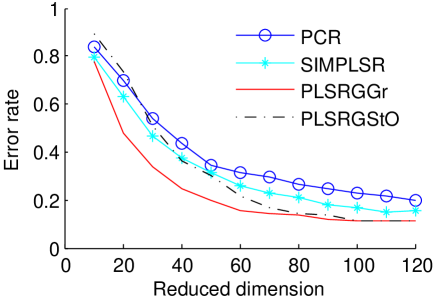
Figure 1: Recognition error (%) on AR face database.

Figure 1 reports the experiment results on AR face database. It shows that the recognition performance of our proposed algorithms, PLSRGGr and PLSRGStO, is better than other methods more than 4 percent when reduced dimension is greater than 60. Obviously, PLSRGGr has good performance all the time. This demonstrates that our proposed optimization models and algorithms of PLSR on Riemannian manifold significantly enhances the accuracy. The reason is that calculating PLSR factors as a whole on Riemannian manifolds can obtain the optimal solution.

$c$	PCR	SIMPLSR	PLSRGGr	PLSRGStO
12	33.27$\pm$3.10	26.00$\pm$4.59	$\mathbf{12.00\pm 0}$	20.07$\pm$0.30
13	30.87$\pm$4.66	21.73.00$\pm$4.06	$\mathbf{9.40\pm 0.30}$	15.93$\pm$0.30
14	29.27$\pm$4.79	19.00$\pm$3.82	$\mathbf{8.00\pm 0}$	8.13$\pm$0.60
15	25.87$\pm$4.61	15.80$\pm$3.13	$\mathbf{10.60\pm 0.30}$	10.67$\pm$0

Table 1: Recognition error (%) on Yale face database.

$c$	GDA	DCC	LSRM	PCR	SIMPLSR	PLSRGGr	PLSRGStO
5	-	-	-	23.75	26.25	$\mathbf{18.75}$	$26.25$
6	-	-	-	22.50	15.00	$15.00$	$\mathbf{13.75}$
7	-	-	-	21.25	7.50	$\mathbf{1.25}$	$\mathbf{1.25}$
8	2.50	11.20	5.00	20.00	3.75	$\mathbf{1.25}$	$\mathbf{1.25}$

Table 2: Classification error (%) on ETH-80 database, the error rate in last line is employed for GDA, DCC, LSRM.

Another experiment was conducted on Yale face database. In this experiment, the compared algorithms are PCR, SIMPLSR, PLSRGGr and PLSRGStO, and every algorithm is run 20 times. Table 1 lists the recognition error rates including their mean and standard deviation values with reduced dimensions $c=12,13,14,15$. From the table we can observe that the mean of recognition error rates of PLSRGGr and PLSRGStO is superior to others with a margin of 5 to 14 percentages, and the standard deviation is also smaller. This demonstrates that our proposed methods more robust. The bold figures in the table highlight the best results for comparison.

4.2 Object Classification

Data Preparation

For the object classification tasks, we use the following two public available databases for testing,

• COIL-20 dataset (http://www.cs.columbia.edu/CAVE/software/softlib/coil-20.php);

• ETH-80 dataset (http://www.mis.informatik.tu-darmstadt.de/Research/Projects/categorization/eth80-db.html).

Columbia Object Image Library (COIL-20) contains 1,440 gray-scale images from 20 objects. Each object offers 72 images. 36 images of each object were selected by equal interval sampling as training while the remaining images are for testing.

ETH-80 database (?) consists of 8 categories of objects Each category contains 10 objects with 41 views per object, spaced equally over the viewing hemisphere, for a total of 3280 images. Images are resized to $32\times 32$ pixels with grayscale pixels and vectorized as 1024-dimensional vector. For each category and each object, we model the pose variations by a subspace of the size $m=7$, spanned by the 7 largest eigenvectors from SVD. In our experiments, the Grassmann distance measure between two point $\text{span}(\mathbf{X}),\text{span}(\mathbf{Y})\in Gr(n,m),$ is defined as $\text{dist}(\mathbf{X},\mathbf{Y})=\|\arccos(\text{svd}(\mathbf{X}^{T}\mathbf{Y}))\|_{F}$ which is the F-norm of principal angles (?), $\text{svd}(\mathbf{X}^{T}\mathbf{Y})$ denotes the singular value of $\mathbf{X}^{T}\mathbf{Y}$. We follow the experimental protocol from (?) which is tenfold cross validation for image-set matching.

Classification Performance

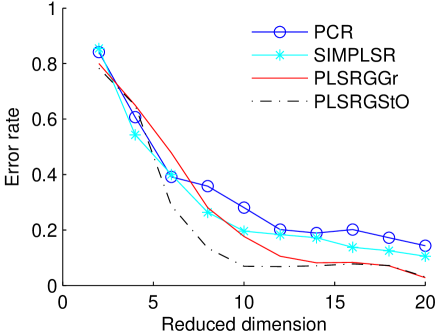
Figure 2: Classification error (%) on COIL20 database.

Figure 2 lists the classification error of four algorithms on COIL-20 database. The classification errors are recorded for the different reduced dimension $c=\{17,18,19,20\}$, respectively. From the results, it can be found that the proposed methods, PLSRGGr and PLSRGStO, outperform their compared non-manifold methods with a margin of 2 to 10 percentages when reduced dimension is greater than 10.

To demonstrate the effectiveness of our regression algorithms on the ETH-80 data set. We compared with several contrast methods. Table 2 reports the experimental results with reduced dimension $c=\{5,6,7,8\}$. The results of GDA (Grassmann discriminant analysis) (?), DCC (Discriminant canonical correlation) (?), LSRM (Least squares regression on manifold) (?) in last line of Table 2 are from (?). Compared with state of-the-art algorithms, our proposed methods, PLSRGGr and PLSRGStO, both outperform all of them.

5 Conclusions

In this paper, we developed PLSR optimization models on both Riemannian manifolds, i.e. generalized Grassmann manifold and product manifold. We also gave optimization algorithms on both the Riemannian manifolds, respectively. Each of new models transforms the corresponding original constrained optimization problem to an unconstraint optimization on Riemannian manifolds. This makes it possible to calculate all the PLSR factors as a whole to obtain the optimal solution. The experimental results show our proposed PLSRGGr and PLSRGStO outperform other methods on several public datasets.

References

- [Absil and Gallivan 2006] Absil, P., and Gallivan, K. 2006. Joint diagonalization on the oblique manifold for independent component analysis. In Acoustics,Speech, and Signal Processing (ICASSP), volume 5.
- [Absil, Mahony, and Sepulchre 2004] Absil, P. A.; Mahony, R.; and Sepulchre, R. 2004. Riemannian geometry of Grassmann manifolds with a view on algorithmic computation. Acta Applicandae Mathematica 80(2):199–220.
- [Absil, Mahony, and Sepulchre 2008] Absil, P. A.; Mahony, R.; and Sepulchre, R. 2008. Optimization Algorithm on Matrix Manifolds. Princeton University Press.
- [Aiken, West, and Pitts 2003] Aiken, L. S.; West, S. G.; and Pitts, S. C. 2003. Multiple linear regression. Handbook of Psychology. 4(19):481–507.
- [Boulesteix and Strimmer 2007] Boulesteix, A., and Strimmer, K. 2007. Partial least squares: A versatile tool for the analysis of high-dimensional genomic data. Briefings in Bioinformatics 8(1):32–44.
- [Boumal et al. 2014] Boumal, N.; Mishra, B.; Absil, P. A.; and Sepulchre, R. 2014. Manopt, a Matlab toolbox for optimization on manifolds. The Journal of Machine Learning Research 15(1):1455–1459.
- [Boyd et al. 2011] Boyd, S.; Parikh, N.; Chu, E.; Peleato, B.; and Eckstein, J. 2011. Distributed optimization and statistical learning via the alternating direction method of multipliers. Foundations and Trends®in Machine Learning 3(1):1–122.
- [Chun and Keles 2010] Chun, H., and Keles, S. 2010. Sparse partial least squares regression for simultaneous dimension reduction and variable selection. Journal of the Royal Statistical Society: Series B (Statistical Methodology) 72(1):3–25.
- [Cunningham and Ghahramani 2014] Cunningham, J. P., and Ghahramani, Z. 2014. Unifying linear dimensionality reduction. arXiv:1406.0873.
- [Edelman, Arias, and Smith 1998] Edelman, A.; Arias, T.; and Smith, S. 1998. The geometry of algorithms with orthogonality constraints. SIAM Journal on Matrix Analysis and Applications 20(2):303–353.
- [Hamm and Lee 2008] Hamm, J., and Lee, D. 2008. Grassmann discriminant analysis: A unifying view on subspace-based learning. In International conference on machine learning, 376–383.
- [Hao, Thelen, and Gao 2016] Hao, X.; Thelen, K.; and Gao, J. 2016. Spatial variability in biomass yield of switchgrass, native prairie, and corn at field scale. Biofuels 108(2):548–558.
- [He, Balzano, and Szlam 2012] He, J.; Balzano, L.; and Szlam, A. 2012. Incremental gradient on the grassmannian for online foreground and background separation in subsampled video. In Computer Vision and Pattern Recognition.
- [Höskuldsson 1988] Höskuldsson, A. 1988. Pls regression methods. Journal of Chemometrics 2(3):211–228.
- [Huang et al. 2005] Huang, X.; Pan, W.; Grindle, S.; and Han, X. 2005. A comparative study of discriminating human heart failure etiology using gene expression profiles. BMC Bioinformatics 6:205.
- [Hulland 1999] Hulland, J. 1999. Use of partial least squares (PLS) in strategic management research: A review of four recent studies. Strategic Management Journal 20(2):195–204.
- [Jolliffe 1982] Jolliffe, I. 1982. A note on the use of principal components in regression. Applied Statistics 31(3):300–303.
- [Jong 1993] Jong, S. D. 1993. SIMPLS: An alternative approach to partial least squares regression. Chemometrics and Intelligent Laboratory Systems 18(3):251–263.
- [Kendall 1957] Kendall, M. G. 1957. A Course in Multivariate Analysis. Griffin, London.
- [Kim, Kittler, and Cipolla 2007] Kim, T. K.; Kittler, J.; and Cipolla, R. 2007. Discriminative learning and recognition of image set classes using canonical correlations. IEEE Transactions on Pattern Analysis and Machine Intelligence 29(6):1005–1018.
- [Leibe and Schiele 2003] Leibe, B., and Schiele, B. 2003. Analyzing appearance and contour based methods for object categorization. In Computer Vision and Pattern Recognition.
- [Liton et al. 2015] Liton, M. A. K.; Helen, S.; Das, M.; Islam, D.; and Karim, M. 2015. Prediction ofaccuratep values of some -substituted carboxylicacids with low cost of computational methods. Journal of Physical & Theoretical Chemistry 12(3):243–255.
- [Lobaugh, West, and McIntosh 2001] Lobaugh, N.; West, R.; and McIntosh, A. 2001. Spatiotemporal analysis of experimental differences in event-related potential data with partial least squares. Sychophysiology 38(3):517–530.
- [Lui 2016] Lui, Y. 2016. A general least squares regression framework on matrix manifolds for computervision. In Riemannian Computing in Computer Vision. Springer International Publishing. 303–323.
- [Mishra and Sepulchre 2014] Mishra, B., and Sepulchre, R. 2014. R3MC: A Riemannian three-factor algorithm for low-rank matrix completion. In Conference on Decision and Control, 1137–1142.
- [Mishra et al. 2014] Mishra, B.; Meyer, G.; Bonnabel, S.; and Sepulchre, R. 2014. Fixed-rank matrix factorizations and Riemannian low-rank optimization. Computational Statistics 29(3):591–621.
- [Ns and Martens 1988] Ns, T., and Martens, H. 1988. Principal component regression in NIR analysis: Viewpoints, background details and selection of components. Journal of Chemometrics 2(2):155–167.
- [Nishimori and Akaho 2005] Nishimori, Y., and Akaho, S. 2005. Learning algorithms utilizing quasi-geodesic flows on the Stiefel manifold. Neurocomputing 67:106–135.
- [Rosipal and Kramer 2006] Rosipal, R., and Kramer, N. 2006. Overview and recent advances in partial least squares. Lecture Notes in Computer Science 3940:34–51.
- [Rosipal 2003] Rosipal, R. 2003. Kernel partial least squares for nonlinear regression and discrimination. Neural Network World 13(3):291–300.
- [Tan et al. 2014] Tan, M.; Tsang, I.; Wang, L.; Vandereycken, B.; and Pan, S. 2014. Riemannian pursuit for big matrix recovery. In International Conference on Machine Learning, volume 32, 1539–1547.
- [Wang et al. 2014] Wang, B.; Hu, Y.; Gao, J.; Sun, Y.; and Yin, B. 2014. Low rank representation on grassmann manifolds. In Asian Conference on Computer Vision.
- [Wang et al. 2016] Wang, B.; Hu, Y.; Gao, J.; Sun, Y.; and Yin, B. 2016. Product grassmann manifold representation and its lrr models. In American Association for Artificial Intelligence.
- [Wegelin 2000] Wegelin, J. 2000. A survey of partial least squares (PLS) methods, with emphasis on the two-block case. Technical report, Department of Statistics, University of Washington, Seattle.
- [Wold et al. 1984] Wold, S.; Ruhe, H.; Wold, H.; and Dunn, W. 1984. The collinearity problem in linear regression. The partial least squares (PLS) approach to generalized inverses. SIAM Journal of Scientific and Statistical Computations 5(3):735–743.
- [Wold 1975] Wold, H. 1975. Path Models with Latent Variables: The NIPALS Approach. Academic Press.
- [Wolf and Shashua 2003] Wolf, L., and Shashua, A. 2003. Learning over sets using kernel principal angles. Journal of Machine Learning Research 4:913–931.
- [Worsley 1997] Worsley, K. 1997. An overview and some new developments in the statistical analysis of PET and fMRI data. Human Brain Mapping 5(4):254–258.