Stochastic dynamics and the predictability of big hits in online videos

Abstract

The competition for the attention of users is a central element of the Internet. Crucial issues are the origin and predictability of big hits, the few items that capture a big portion of the total attention. We address these issues analyzing 10 million time series of videos’ views from YouTube. We find that the average gain of views is linearly proportional to the number of views a video already has, in agreement with usual rich-get-richer mechanisms and Gibrat’s law, but this fails to explain the prevalence of big hits. The reason is that the fluctuations around the average views are themselves heavy tailed. Based on these empirical observations, we propose a stochastic differential equation with Lévy noise as a model of the dynamics of videos. We show how this model is substantially better in estimating the probability of an ordinary item becoming a big hit, which is considerably underestimated in the traditional proportional-growth models.

I Introduction.

YouTube is a representative example of online platforms in which items (videos in this case) compete for the attention of users Simon (1971); Wu and Huberman (2007); Salganik et al. (2006). The popularity of videos vary by orders of magnitude, resembling the fat-tailed distributions that have been reported in other online systems Huberman et al. (2009); Miotto and Altmann (2014a); Weng et al. (2012), in income and wealth Pareto (1898 (1964), in finance Mandelbrot (1963), and in disciplines such as ecology, earth science, and physics Clauset et al. (2009). The origin of such fat-tailed distributions is a century-old problem that lies at the heart of complex-systems science Yule (1925); Gibrat (1931); Mandelbrot (1960); Simon and Bonini (1958); Simkin and Roychowdhury (2011); Perc (2014). At the core of the different proposed models lies the idea that the current popularity (wealth) determines the future popularity gain (income) and enhances the inequality (rich-get-richer). Indeed, such (linear) proportional growth is the essential ingredient of Gibrat’s law (used to describe the growth of firms Gibrat (1931); Simon and Bonini (1958) and cities Gabaix (1999)), the Yule-Simon model (to model species genera Yule (1925) and language Simon (1955); Gerlach and Altmann (2013)), scientific memes Kuhn et al. (2014) and the preferential attachment model of network growth Barabási and Albert (1999). Proportional growth suggests that the big hits are very predictable because they originate from early advantages that are amplified over time.

The application of growth models to describe the popularity of online items bring new opportunities and challenges. On the one hand, due to the increasing availability of datasets, it becomes possible to compare models with an unprecedent accuracy. On the other hand, the expectations we have of the models are higher. For instance, a central question is to forecast and identify the origins of the big hits Wang et al. (2013); Watts (2011), the most successful videos which capture most of the attention and produce most of the revenue through advertisement. To address this and other questions, the characterization of the heavy-tailed distribution of aggregated activity is not enough. One has to: (i) improve the description of the dynamics of individual items; and (ii) go beyond the average growth and analyze the stochastic fluctuations Maillart et al. (2008); Ratkiewicz et al. (2010). The importance of these factors is illustrated in Fig. 1, where we show trajectories (views vs. time) of videos with the same early success (the same number of views, 3 days after publication). We see that trajectories quickly spread and that many trajectories with a weak start become popular in time. This suggests that big hits have a low predictability (i.e., they are hard to anticipate).

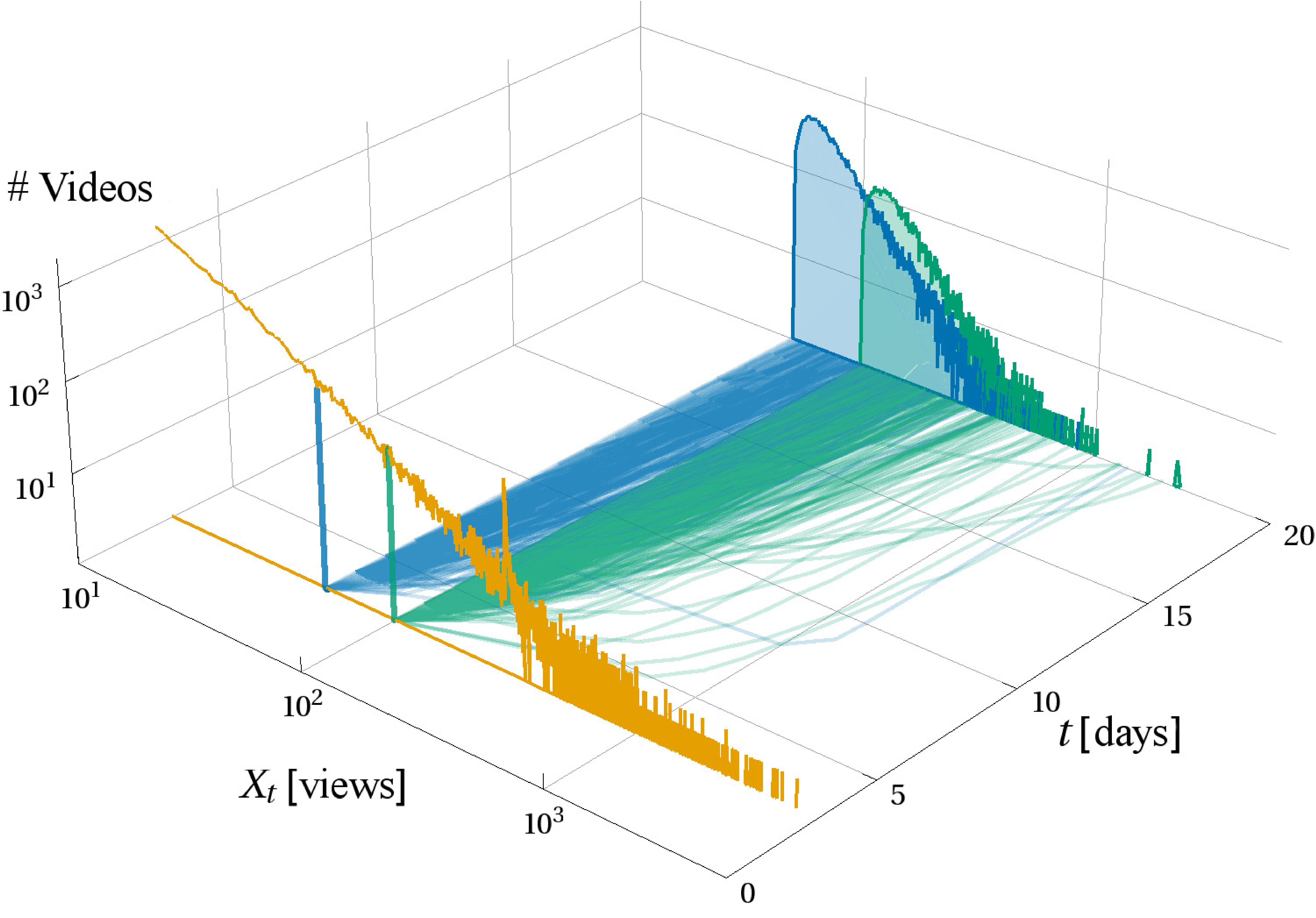
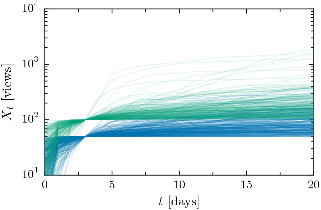
Figure 1: Evolution of videos’ views $X_{t}$ as a function of the time $t$ after publication. After $t=3$ days the distribution of views is already heavy-tailed (orange histogram). Videos having initially the same amount of views show very distinct evolutions. This is illustrated here by highlighting two group of videos with the same number of views at $t=3$ (blue $X_{t=3}=50$ and green $X_{t=3}=100$). Each line (at the bottom and in the right plot) corresponds to the trajectory of one video. On the back, the histograms of the two groups of videos at $t=20$ days are shown.

In this article, we investigate the predictability of big hits using stochastic models of individual items. Predictability is the possibility of anticipating the future based on present information and we confront the predictability expected from models to observations in the data. We compare traditional growth models to data ($X_{t}$, views over time) of more than 10 million YouTube videos. We find that previously proposed models are unable to correctly account for the (random) fluctuations observed in the data, which we find to be described by a Lévy-stable distribution. We propose and validate a stochastic model that explains such reduced predictability by incorporating both proportional growth and Lévy noise. This shows that, even if present, proportional growth is not the only responsible for the origin of fat-tailed distributions. Finally we show that our model substantially improves the prediction of the probability of big hits, but that unexpected big hits have an even higher probability in real data due to temporal correlations not accounted by this class of models.

II Theoretical Framework

YouTube is a website where videos generated by third parties are shared. It is the third most visited website of all Internet. We collected more than 10 million time series of the daily number of views of videos published between Dec 2011 and Mar 2013 Miotto and Altmann (2014b). The number of views a video receives depends on the interplay between its content and various factors. Videos related to ongoing events are strongly influenced by their development, its media coverage, and other factors exogenous to the online activity of users. Videos are also influenced by endogenous factors, such as the sharing and recommendation in online media, generating cascades of activity in the social network Sornette et al. (2004); Watts (2002). Additionally, a video can be viewed by following a link from a related video, i.e. hopping through the videos’ network which changes continuously according to YouTube’s recommendation and promotion algorithms. The interplay and feedback between these and other factors lead to the complex dynamics we observe in the time series. Modeling specific factors Chatzopoulou et al. (2010) and differentiating between them (e.g., between exogenous and endogenous factors Crane and Sornette (2008); Sornette et al. (2004); Ghanbarnejad et al. (2014)) are topics of recent research. This approach is difficult to be pursued because it requires detailed information of user activities and the possibility of isolating the factors. Instead, here we aim at a coarse-grained description of the dynamics of attention in which the combination of the different factors described above are effectively accounted by deterministic and stochastic terms.

Let $X_{t}$ be the cumulative number of views that a video received in the first $t$ days after its release. A very general stochastic model for the growth of $X_{t}$ in $t$ is the diffusion process Risken (1984); Maillart et al. (2008); Mollgaard and Mathiesen (2015)

$$dX_{t}=\mu(t,X_{t})dt+\sigma(t,X_{t})dW_{t},$$ (1)

where $W_{t}$ is a Wiener process ($\langle W_{t}\rangle=0$ and $\langle W_{t}^{2}\rangle=dt$), $\mu(t,X_{t})$ is the average growth, and $\sigma(t,X_{t})$ scales the fluctuations; an additional cutoff in $dW_{t}$ is added to ensure that $dX_{t}>0$. We consider all videos to be indistinguishable so that variations in the behavior of videos with the same $X_{t}$ should be accounted by the stochastic term $\sigma(t,X_{t})dW_{t}$. Extensions of our model could consider $\mu(t,X_{t})$ and $\sigma(t,X_{t})$ to depend on properties of the video and on $X_{t^{\prime}}$ for $t^{\prime}<t$.

III Data analysis

We now analyze the data in order to identify the functions $\mu(t,X_{t})$ and $\sigma(t,X_{t})$. Since the minimum resolution of our data is $\Delta t=1$ day, the models we propose aim to fit the quantity $\Delta X_{t}=X_{t+1}-X_{t}$, the number of views obtained exclusively in the day $t+1$. We first focus on the deterministic term of Eq. (1), $\mu(t,X_{t})$. In linear proportional growth models the average growth is proportional to the views, $\mu(t,X_{t})=\mu_{t}X_{t}$, where the temporal dependence on $\mu_{t}$ accounts for the decay in the attention gain Wu and Huberman (2007); this decay is very strong in the first weeks, so we will focus on the days up to $t=30$.

This condition is consistent with our data: in Fig. 2(a) we see for a fixed $t$, that the dependence of the conditional average $\langle\Delta X_{t}|X_{t}\rangle$ (computed in windows of $N$ videos) with $X_{t}$ is roughly a line with slope $1$, a standard method to check for proportional growth Newman (2001); Perc (2014).

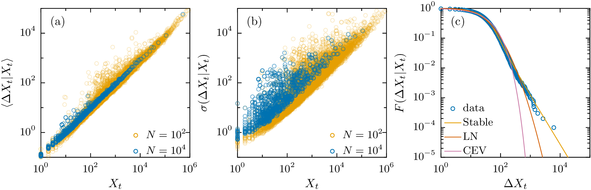
Figure 2: Average and fluctuations in the growth of YouTube Videos. (a) Mean $\langle\Delta X_{t}\rangle$ and (b) standard deviation $\sigma(\Delta X_{t}$) for videos with $X_{t}$ views $t=3$ days after publication. Both $\langle\ldots\rangle$ and $\sigma$ are computed in windows centered at $X_{t}$ and containing $N$ items (see legend). (c) Complementary cumulative density function $F(\Delta X_{t}|X_{t})$ for $X_{t}\in[499,513]$ and $t=3$. Data (blue circles) is compared with fits of three distributions (S: Lévy-stable, LN: Lognormal, CEV: Constant Elasticity of Variance) and confirms the existence of heavy tails which are best described by the Lévy distribution.

We now repeat the analysis for the stochastic term $\sigma(X_{t},t)$ of Eq. (1). A natural proposal for $\sigma$ is $\sigma(X_{t},t)=\sigma_{t}X_{t}^{\beta}$ Mollgaard and Mathiesen (2015), where the $\beta$ parameter allows us to model a possible fluctuations’ scaling, in the form of the Taylor’s Law Eisler et al. (2008). In particular, the $\beta=1$ case used in Ref. Maillart et al. (2008), is equivalent to $Y_{t}=\ln X_{t}$ exhibiting constant fluctuations, and corresponds to a Geometric Brownian Motion. The simplest way to evaluate the stochastic term in this context is to repeat what was done for the mean and measure the standard deviation $\sigma$ in a window of $N$ items centered around $X_{t}$ Maillart et al. (2008). This is equivalent to the standard estimation of the drift and diffusion coefficients in a Fokker-Planck Equation Friedrich and Peinke (1997). Results in Fig. 2(b) confirm the roughly linear scaling in the double logarithmic scale, in agreement with $\sigma(X_{t},t)\propto X_{t}^{\beta}$ with $\beta\approx 1$. However, in opposite to the case of $\mu(X_{t},t)$ shown in panel (a), the data show strong fluctuations across $X_{t}$ and depend on the sample size $N$ (the larger the $N$ the larger the measured $\sigma$).

The observations above motivate us to look at the full probability distribution $\mathbb{P}(\Delta X_{t}|X_{t})$ Amaral et al. (1998). In Fig. 2(c) we see in the particular histogram $\mathbb{P}(\Delta X_{3}|X_{3}\approx 500)$, that the distribution has a heavy tail; this explains the observation that $\sigma$ grows with $N$, i.e. $\mathbb{P}(\Delta X_{t}|X_{t})$ has a diverging second moment Bouchaud and Georges (1990). Heavy-tailed fluctuations of $\Delta X_{t}$ may still be compatible with Eq. (1) if one considers that the temporal interval used in our analysis is not infinitesimal $\Delta t=1$ day $\gg dt$; in deed, Gaussian fluctuations are expected only when $\Delta t\rightarrow 0$. In this case, the stochastic differential equation has to be integrated up to $\Delta t$, so the fluctuations predicted from Eq. (1) can be Lognormal (for $\beta=1$) or a distribution arising from the Constant Elasticity of Variance model (CEV, for $\beta\neq 1$) Chen and Lee (2010), as shown in App. A. Besides Eq. (1), classical models associated with Gibrat’s law (Champernowne-Gabaix or Yule-Simon) predict $\mathbb{P}(\Delta X_{t}|X_{t})$ to have either short tails or Lognormal distributions (see App. B). Beyond the Lognormal and CEV distributions, which follow from Eq. (1), we consider also the Lévy-stable distribution (S) because it originates from the generalized Central Limit Theorem for variables without finite variance Zolotarev (1986). In Fig. 2(c) we show the fits of discretized versions of these 3 distributions to the particular histogram discussed above. The best fit is obtained by the (completely asymmetric) Lévy-stable distribution (with a difference in the Bayes Information Criterion Schwarz (1978); noteBIC , BIC, of 178 and 175, with respect to the Lognormal and CEV models). This result, which is confirmed below for different $X_{t}$ and $t$, indicates that the fluctuations observed in the data are not compatible with the Wiener process $W_{t}$ in Eq. (1), and that the analysis of the mean and standard deviation done for Fig. 2(a) and (b) may be not enough to define the functions of Eq. 1.

IV Alternative Model

Motivated by the better fit of the Lévy distribution and by the linear scaling of $\mu$ and $\sigma$ with $X_{t}$ (as shown in Fig. 2), we propose as an improvement of Eq. (1) Janicki and Weron (1993)

$$dX_{t}=\mu_{t}X_{t}dt+(a_{t}X_{t}+b_{t})dL_{t},$$ (2)

where $L_{t}$ is an $\alpha$-stable Lévy process, analogous to the Wiener process, except that the distribution of $dL_{t}$ follows a Lévy-stable distribution with index $\alpha$, asymmetry $1$, location parameter $0$ and scale $1$ (using parametrization $1$ of Ref. Nolan (2012)). A cutoff in the noise term is added as above to ensure $dX_{t}\geq 0$, so $\langle dL_{t}\rangle>0$ and $\langle\Delta X_{t}\rangle$ is not given alone by the deterministic term $\mu_{t}X_{t}$ (even if $dL_{t}$ is understood in the Ito sense, as we do here Øksendal (2003)). The parameters $\alpha,\mu,a,$ and $b$ depend on time $t$ ($b_{t}$ is important only for small $X_{t}$ and $t$). Table 1 summarizes all models.

Name	$\mathbb{P}(\Delta X_{t}|X_{t})$ functional form	Parameters
LN	Lognormal	$\mu_{t}$, $\sigma_{t}$
CEV	CEV	$\mu_{t}$, $\sigma_{t}$, $\beta_{t}$
S	Lévy-stable	$\alpha_{t}$, $\mu_{t}$ $a_{t}$, $b_{t}$

Table 1: Sumsmary of models, see App. A for details.

V Improved data analysis

We now discuss how to determine the parameters of the two models derived from Eq. (1) and of the alternative model in Eq. (2) and to test which model best describes the data. The likelihood $\mathcal{L}_{t}$ of the models, for a fixed day $t$, is the product of the likelihoods of each distribution of $\Delta X_{t}$ conditioned on $X_{t}$ with respect to the parameters of the model $\theta$ as

$$\ln\mathcal{L}_{t}=\sum_{X_{t}}\sum_{\Delta X_{t}}N(\Delta X_{t},X_{t})\ln f(\Delta X_{t}|\theta,X_{t}),$$ (3)

where $N(\Delta X_{t},X_{t})$ is the observed number of videos with a given $\Delta X_{t},X_{t}$, and $f$ is the probability density function proposed by the models. The best parameters $\theta$ are obtained maximizing $\ln\mathcal{L}_{t}$ and the models are compared based on their (maximum) Likelihood, penalizing the addition of parameters (using the BICnoteBIC ). The distributions $f$ we test are the same as above: Lognormal (LN) and Constant Elasticity of Variance (CEV), obtained from Eq. (1), and Lévy-stable (Stable), obtained from Eq. (2). The latter is the $f$ resulting from Eq. (2) because, since it seems to be a better fit to the data, we consider in this model that the time step $\Delta t$ is small such that $\Delta X_{t}\approx dX_{t}$, making the distribution to be fitted exactly the Lévy. Each of the distributions $f$ has different parameters that depend on $\theta$ and $X_{t}$, as summarized in Tab. 1 and detailed in App. A. Our approach based on Eq. (3) considers all conditional distributions $\mathbb{P}(\Delta X_{t}|X_{t})$, avoiding the difficulties and arbitrary choices involved in the grouping of data in windows as done in previous estimations and in Fig. 2.

The application of the analysis described above to the YouTube data leads to significant evidence in favor of the Lévy-stable model, Eq. (2). Figure 3 shows how the this model allows for the collapse of the many $\mathbb{P}(\Delta X_{t}|X_{t})$ in a single curve, well described by a Lévy stable curve. More formally, the BIC noteBIC difference of the Stable model with respect to the other models is above $10^{5}$ for all $0\leq t\leq 30$ (inset of Fig. 3), indicating very strong statistical support for our model.

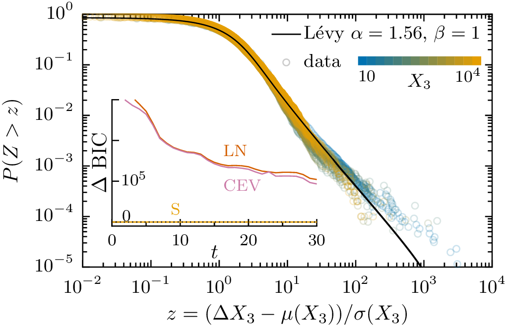
Figure 3: Agreement of the model with respect to data. Main panel: complementary cumulative distribution of the views rescaled by the fitted parameters for $t=3$. The rescaled histograms $\mathbb{P}(\Delta X_{3}|X_{3})$ are plotted as points, where each color corresponds to a different value of $X_{3}$; the black line is the Lévy-stable distribution with location $0$ and scale $1$. Inset: BIC difference with respect to the S modelnoteBIC .

V.1 Dependence of parameters with respect to $t$

The parameters of the S model (Eq. 2) are explicitly time dependent, so we repeat the previous procedure for each of the days considered. In Fig. 4 the values of these are shown for the first 30 days after the publication of the videos. The parameters show a strong dependence in $t$ in the the first week. In particular, $\mu_{t}$ decays in this period (reflecting a decay in the gain of views) and $\alpha_{t}\approx 1.75$ for $t>5$. It is worth to be noted is that the value of $\mu_{t}$ becomes negative; while apparently in contradiction with the positive slope of $\langle\Delta X_{t}|X_{t}\rangle$ (see Fig. 2(a)), it has to be recalled that the distribution is truncated at $\Delta X_{t}=0$. The values of the averages from the data can be recovered through an exact, numerical computation.

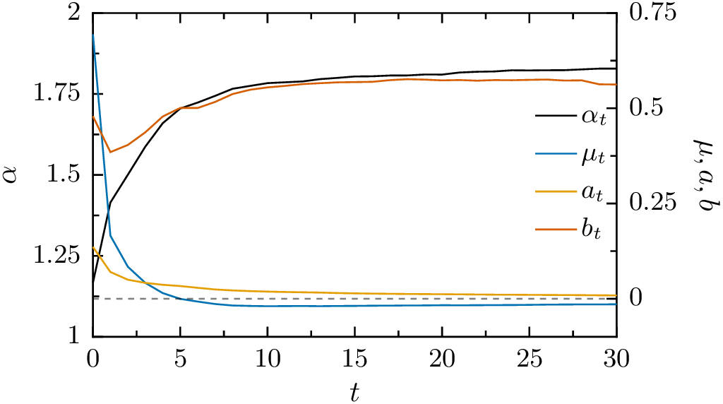
Figure 4: Evolution of the parameters for the S model, Eq. (2), in the first $30$ days after the release.

If wanted, a model of the temporal dependence of $\alpha_{t},\mu_{t},a_{t},b_{t}$ can be introduced; in that case, it is possible to sum the likelihoods in Eq. (3) over $t$ and therefore to reduce the number of parameter of the models by avoiding independent fittings for each $t$.

Altogether, these analysis support our proposal of stochastic differential equation with Lévy noise, Eq. (2), to describe the dynamics of popularity in YouTube.

VI Prediction of big hits

We now focus on the estimation of the probability of an item becoming a big hit after a given time. We define as a big hit at time $t$ the top $q\%$ videos with highest $X_{t}$ ($X_{t}>x_{t}^{q}$). We are particularly interested in estimating the probability $P(X_{t}>x_{t}^{q}|X_{t_{0}}=x_{0})$ of videos that are not big hits at time $t_{0}<t$ (i.e., $x_{0}<x_{t_{0}}^{q})$ becoming big hits at time $t$. This probability quantifies how unpredictable the system is. For instance, in a deterministic (proportional growth) model, the rank of the videos does not change and therefore such probability is zero. A positive probability is thus a measure of the deviation of such perfect predictability.

As an example, we select the videos that had 100 views one day after publication, $X_{1}=100$, which belong to a rank of $q\approx 15\%$. We are interested in the probability of these videos having $X_{t}\gg 100$ at $t>1$. To obtain the expectations of the models, we computed $P(X_{t}|X_{1}=100)$ iteratively from $P(dX_{s}|X_{s})$ for $s=1,\ldots t$, using $X_{1}=100$ and the $t$-dependent parameters estimated in the previous section. The results shown in Fig. 5(main panel) for $t=6$ confirm that the Lévy-stable model predicts a substantially higher probability for large $X_{t}$ than alternative models. In order to investigate the temporal dependence, we focus on the probability of the videos improving their rank and being by day $t$ in the top $q=5\%$, using the previously computed probabilities from the models and the thresholds $x_{t}^{q}$ estimated from data. The results are summarized in Fig. 5(inset) and show that the Lévy-stable model succeeds in estimating this probability in the short-term, while for the long-term the data shows an even higher probability (mixing of ranks). The other models assign a video a substantially lower possibility of becoming a big hit, an effect of their highly predictable dynamics. The fact that our model provides a good account for short-time intervals but not in the long run suggests the existence of correlations in the attribution of views that span multiple days and that are not accounted by our assumption of an independent noise.

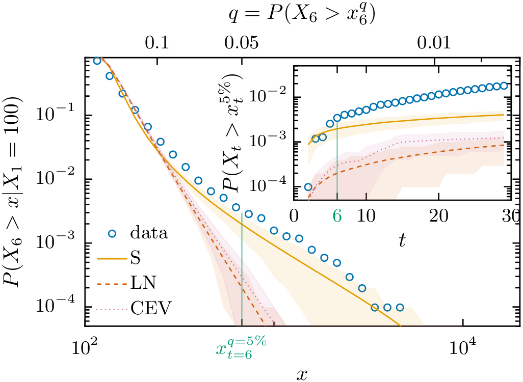
Figure 5: Probability of videos becoming a big hit. Performance of the models evolved in time with respect to data; the selected videos had $100$ views $1$ day after their publication. Main panel: amount of videos that exceed a threshold $x$ at $t=6$. In the top axis, the quantiles $q$ are indicated. Inset: amount of videos that enter into the $5\%$ most viewed. Shaded areas: 95% confidence intervals, by bootstrapping.

VII Discussion and Conclusion

Our finding that the growth of views in YouTube is governed by both linear proportional growth and Lévy fluctuations has important consequences for the mathematical modeling of complex systems. First, it shows that, even if proportional growth is present, it cannot be attributed as the responsible for the origin of the heavy tails because this is a feature already present in the fluctuations. Second, the use of Gaussian-based stochastic equations, such as Eq. (1) or traditional Fokker-Planck equations, overestimate the predictability of videos, by neglecting the mobility of popularity. We showed that better results are obtained in YouTube using a stochastic equation with Lévy noise, Eq. (2), an approach that has been previously used in Physics Janicki and Weron (1993), climate research Ditlevsen (1999), and finance Mandelbrot (1963). Our work indicates that this formalism, and possibly also kinetic equations of the fractional type Metzler et al. (1999); Brockmann and Sokolov (2002), should be considered in problems involving the dynamics of social-media items and, more generally, in models of the economy of attention.

Our results bring new insights on the attention economy of the Internet. The fact that the multiple factors affecting the popularity of videos can be effectively modeled by a Lévy-stable distribution shows that the decision of different individuals are correlated to each other and lead itself to strong fluctuations. The Lévy-stable distribution is invariant under convolution, i.e. if $X_{1}$,$X_{2}$ are stable, also $X_{1}+X_{2}$ is stable, and therefore it may naturally appears when multiple processes with diverging moments are combined (e.g., bursty activity patterns that characterize online social media). One challenge for future work is to identify mechanistic models of the spreading of information on the Internet (e.g., models in which viral items spread through a social network) that are compatible with these fluctuations Watts (2002); Maillart et al. (2008); Ratkiewicz et al. (2010). The presented analysis of fluctuations are enabled by the large availability of data in YouTube videos and we expect similar results to hold also in more general systems in which items compete for the attention of users.

Appendix A Models

We compare the data collected with the distribution predicted by a series of simple models: from Eq. (1), we derive the Lognormal (LN) and Constant Elasticity of Variance (CEV) models; from Eq. (2) we derive the Lévy-stable model (S). To compare with data, we compute the distributions of $X_{t+1}$ of the different models. Note that for the LN and CEV models, these distributions are the result of integrating Eq. (1) over a period of one day, while for the S models, this integration is not performed, i.e. we assume that in the period of one day the distribution of $X_{t+1}$ is essentially the one of the noise.

A.1 Lognormal (LN)

The LN model is defined by considering a linear scaling of the noise term in Eq. (1)

$$dX_{t}=\mu_{t}X_{t}dt+\sigma_{t}X_{t}dW_{t}$$ (4)

We integrate this equation for a time equal to 1 day (where we consider $\mu_{t}$ and $\sigma_{t}$ constant), such that $X_{t+1}$ is distributed lognormally, with a probability density function

$$\mathbb{P}(X_{t+1}=x|X_{t}=x_{0})=\frac{\exp\left(-(\log x-(\log x_{0}+\mu_{t}-\sigma_{t}^{2}/2))^{2}/(2\sigma_{t}^{2})\right)}{\sqrt{2\pi}\sigma_{t}x}$$ (5)

$\Delta X_{t+1}=X_{t+1}-X_{t}$ is distributed also lognormally, since $X_{t}$ is fixed, but a truncation at 0 is necessary. Since the data is distributed on the natural numbers, we discretize as well the distribution, normalizing by the sum of the PDF over its new domain.

A.2 Constant Elasticity of Variance (CEV)

If instead of Eq. (4) the equation

$$dX_{t}=\mu_{t}X_{t}dt+\sigma_{t}X_{t}^{\beta}dW_{t}$$ (6)

is used, we have to use the distribution of the Constant Elasticity of Variance process (CEV), described in Ref. Chen and Lee (2010). When $\beta<1$, it has the form

$$\mathbb{P}(X_{t+1}=x|X_{t}=x_{0})=2(1-\beta)k^{\frac{1}{2(1-\beta)}}\left(xz^{1-4\beta}\right)^{\frac{1}{4(1-\beta)}}e^{-x-z}I_{\left|\frac{1}{2(1-\beta)}\right|}\left(2\sqrt{xz}\right)$$ (7)

with

$$k =\frac{\mu}{\sigma^{2}(1-\beta)(e^{2\mu(1-\beta)}-1)}$$

$$x =k(x_{0}e^{\mu})^{2(1-\beta)}$$

$$z =kx^{2(1-\beta)}$$

where $I$ is the modified Bessel function of the first kind. The expression simplifies using the substitution $p=2(1-\beta)$:

$$\mathbb{P}(X_{t+1}=x|X_{t}=x_{0})=pk^{\frac{1}{p}}\left(xz^{2p-3}\right)^{\frac{1}{2p}}e^{-x-z}I_{\left|\frac{1}{p}\right|}\left(2\sqrt{xz}\right)$$ (8)

with

$$k =\frac{2\mu}{\sigma^{2}p(e^{\mu p}-1)}$$

$$x =kx_{0}^{p}e^{\mu p}$$

$$z =kx^{p}$$

When $\beta>1$, the distribution is the same as above but multiplied by $-1$. Note that the $\beta$ parameter is the exponent of the power-law tail that the distribution has asymptotically. Here we also subtract $X_{t}$ to obtain a distribution of $\Delta X_{t}$, which we also truncate, discretize, and normalize.

A.3 Lévy-stable (S)

In the S-model, defined in Eq. (2), $dX_{t}$ is Lévy-stable distributed with location parameter $m=\mu_{t}x_{0}$, scale parameter $s=a_{t}x_{0}+b_{t}$, asymmetry $\beta_{L}=1$ and its tail decays as an $\alpha$ power of $dX_{t}$. These parameters correspond to the parametrization $1$ of Ref. Nolan (2012), where the characteristic function of $dX$ (there is no explicit form of the Lévy probability distribution function), $\phi_{dX}(k)$ is given by

$$\log\phi_{dX}(k)=\begin{cases}imk-s^{\alpha}|k|^{\alpha}\left[1+i\beta_{L}\,\tan\left(\frac{\pi\alpha}{2}\right)\text{sign}(k)\right]&\quad\alpha\neq 1\\ imk-s|k|\left[1+i\beta_{L}\frac{2}{\pi}\text{sign}(k)\log(|k|)\right]&\quad\alpha=1\end{cases}$$ (9)

We consider $\Delta X_{t}\approx dX_{t}$, and the parameters absorb the dependence on $\Delta t$. In order to get the distribution $\mathbb{P}(X_{t+1}=x|X_{t}=x_{0})$, the characteristic function has to be transformed to the real space, translated on the $X_{t+1}$ axis by an amount $x_{0}$, and then truncated at $X_{t+1}=x_{0}$, discretized, and normalized.

Numerically, the Lévy distribution is computed as:

• the characteristic function (its Fourier transform) is inverted numerically on a grid in$\alpha\in(0.5,2)$ and $\beta\in(0,1)$ (with a resolution of $0.05$, values of $\alpha$ below $0.5$ are very unlikely and for $\beta<0$ the distribution can be computed from the one of $-\beta$ using symmetry);

• for general values $\alpha,\beta$, we compute the distribution as an interpolation of the values on the grid (using the Catmull-Rom cubic splines).

• the numerical integration often becomes unstable in the tails of the distribution (large $x$). In order to avoid this problem, we use the power-law approximation described in Ref. Newman (2001) to describe the distribution beyond a threshold.

We provide the code of this procedure in the package PyLevy Miotto (2016). It contains routines to compute the PDF of the Lévy distribution and to fit it.

Appendix B Fluctuations expected from existing models

Here we discuss the form that $\mathbb{P}(\Delta X_{t}|X_{t})$ has for the classical linear proportional growth models. There are basically two schemes of implementing linear proportional growth in order to get heavy-tailed distributions:

• Scheme 1: Champernowne Champernowne (1953) introduces a lower positive limit to $X$. A master equation is defined to regulate the transitions to different states (amount of views), which eventually leads to a stationary distribution with a power-law tail. This argument was formalized and popularized in Refs. Kesten (1973); Gabaix (1999), using a linear stochastic differential equation (as Geometric Brownian Motion, GBM) which, in the limit of long time, converges to a heavy tailed distribution; note that in this scheme, all items start with the same initial condition.

• Scheme 2: Yule and Simon Yule (1925); Simon (1955) design a scheme where views are added to different items while at the same time new items are introduced, resulting in a power law distribution. This is basically the model known as preferential attachment Barabási and Albert (1999) in the context of network growth. Here the items start in different conditions, since the system is growing in the number of items, hence the first ones are privileged.

We focus on the transition probability $\mathbb{P}(\Delta X_{t}|X_{t})$. Scheme 1 (GBM) is a mechanism that leads to a heavy-tailed distribution asymptotically, but also relies on the possibility of negative growth rates $dX_{t}$, which is not realistic in the context of videos’ views, and more generally in the context of cumulative allocation of attention. For an infinitesimal increase of time ($\Delta t\approx dt$), the distribution is Normal, but if a finite time interval is considered ($\Delta t\gg dt$), the integration of the model results in a Lognormal distribution.

The Scheme 2, instead, is fundamentally different and can be thought of as a Polya Urn process where at a given time $t_{0}$, a number of views $N$ is assigned to a set of videos $M$ that has exactly $x_{0}$ views already. The probability of assigning a view to a particular video is, of course, proportional to the amount of views each video has. The distribution $\mathbb{P}(\Delta X_{t}|X_{t})$ of views among the videos is of the Beta Binomial type, with means

$$\mathbb{E}_{BB}(\Delta X_{t}|X_{t}=x_{0})=\frac{N}{M}$$ (10)

and variance

$$\mathbb{V}_{BB}(\Delta X_{t}|X_{t}=x_{0})=\frac{N(M-1)(Mx_{0}+N)}{M^{2}(Mx_{0}+1)}$$ (11)

and can be roughly approximated by a Normal distribution with same mean and variance. The variance scales in two regimes because of the $Mx_{0}+N$ term: when $x_{0}\lesssim N/M$, $\sigma\propto x_{0}^{-1/2}N/M$, and when $x_{0}\gtrsim N/M$, $\sigma\propto\sqrt{N/M}$. Notice though, that the amount of views allocated, $N$, is not independent. In fact, since growth is linear, we expect $N\propto x_{0}M$, so we have in this particular case $\sigma\propto x_{0}^{1/2}$.

In conclusion, for Scheme 1, we expect normal or Lognormal distributions of $\Delta X_{t}$, depending on the choice of whether integrating over a finite time or not, while for Scheme 2 we expect approximately normal distributions, with variance scaling as $X_{t}$.