Learning HMMs with Nonparametric Emissions via
Spectral Decompositions of Continuous Matrices

Abstract

Recently, there has been a surge of interest in using spectral methods for estimating latent variable models. However, it is usually assumed that the distribution of the observations conditioned on the latent variables is either discrete or belongs to a parametric family. In this paper, we study the estimation of an $m$-state hidden Markov model (HMM) with only smoothness assumptions, such as Hölderian conditions, on the emission densities. By leveraging some recent advances in continuous linear algebra and numerical analysis, we develop a computationally efficient spectral algorithm for learning nonparametric HMMs. Our technique is based on computing an SVD on nonparametric estimates of density functions by viewing them as continuous matrices. We derive sample complexity bounds via concentration results for nonparametric density estimation and novel perturbation theory results for continuous matrices. We implement our method using Chebyshev polynomial approximations. Our method is competitive with other baselines on synthetic and real problems and is also very computationally efficient.

1 Introduction

Hidden Markov models (HMMs) [1] are one of the most popular statistical models for analyzing time series data in various application domains such as speech recognition, medicine, and meteorology. In an HMM, a discrete hidden state undergoes Markovian transitions from one of $m$ possible states to another at each time step. If the hidden state at time $t$ is $h_{t}$, we observe a random variable $x_{t}\in\mathcal{X}$ drawn from an emission distribution, $O_{j}=\mathbb{P}(x_{t}|h_{t}=j)$. In its most basic form $\mathcal{X}$ is a discrete set and $O_{j}$ are discrete distributions. When dealing with continuous observations, it is conventional to assume that the emissions $O_{j}$ belong to a parametric class of distributions, such as Gaussian.

Recently, spectral methods for estimating parametric latent variable models have gained immense popularity as a viable alternative to the Expectation Maximisation (EM) procedure [2, 3, 4]. At a high level, these methods estimate higher order moments from the data and recover the parameters via a series of matrix operations such as singular value decompositions, matrix multiplications and pseudo-inverses of the moments. In the case of discrete HMMs [2], these moments correspond exactly to the joint probabilities of the observations in the sequence.

Assuming parametric forms for the emission densities is often too restrictive since real world distributions can be arbitrary. Parametric models may introduce incongruous biases that cannot be reduced even with large datasets. To address this problem, we study nonparametric HMMs only assuming some mild smoothness conditions on the emission densities. We design a spectral algorithm for this setting. Our methods leverage some recent advances in continuous linear algebra  [5, 6] which views two-dimensional functions as continuous analogues of matrices. Chebyshev polynomial approximations enable efficient computation of algebraic operations on these continuous objects [7, 8]. Using these ideas, we extend existing spectral methods for discrete HMMs to the continuous nonparametric setting. Our main contributions are:

1. We derive a spectral learning algorithm for HMMs with nonparametric emission densities. While the algorithm is similar to previous spectral methods for estimating models with a finite number of parameters, many of the ideas used to generalise it to the nonparametric setting are novel, and, to the best of our knowledge, have not been used before in the machine learning literature.

2. We establish sample complexity bounds for our method. For this, we derive concentration results for nonparametric density estimation and novel perturbation theory results for the aforementioned continuous matrices. The perturbation results are new and might be of independent interest.

3. We implement our algorithm by approximating the density estimates via Chebyshev polynomials which enables efficient computation of many of the continuous matrix operations. Our method outperforms natural competitors in this setting on synthetic and real data and is computationally more efficient than most of them. Our Matlab code is available at github.com/alshedivat/nphmm.

While we focus on HMMs in this exposition, we believe that the ideas presented in this paper can be easily generalised to estimating other latent variable models and predictive state representations [9] with nonparametric observations using approaches developed by Anandkumar et al. [3].

Related Work: Parametric HMMs are usually estimated using maximum likelihood principle via EM techniques [10] such as the Baum-Welch procedure [11]. However, EM is a local search technique, and optimization of the likelihood may be difficult. Hence, recent work on spectral methods has gained appeal. Our work builds on Hsu et al. [2] who showed that discrete HMMs can be learned efficiently, under certain conditions. The key idea is that any HMM can be completely characterised in terms of quantities that depend entirely on the observations, called the observable representation, which can be estimated from data. Siddiqi et al. [4] show that the same algorithm works under slightly more general assumptions. Anandkumar et al. [3] proposed a spectral algorithm for estimating more general latent variable models with parametric observations via a moment matching technique.

That said, there has been little work on estimating latent variable models, including HMMs, when the observations are nonparametric. A commonly used heuristic is the nonparametric EM [12] which lacks theoretical underpinnings. This should not be surprising because EM is a maximum likelihood procedure and, for most nonparametric problems, the maximum likelihood estimate is degenerate [13]. In their work, Siddiqi et al. [4] proposed a heuristic based on kernel smoothing, with no theoretical justification, to modify the discrete algorithm for continuous observations. Further, their procedure cannot be used to recover the joint or conditional probabilities of a sequence which would be needed to compute probabilities of events and other inference tasks.

Song et al. [14, 15] developed an RKHS-based procedure for estimating the Hilbert space embedding of an HMM. While they provide theoretical guarantees, their bounds are in terms of the RKHS distance of the true and estimated embeddings. This metric depends on the choice of the kernel and it is not clear how it translates to a suitable distance measure on the observation space such as an ${L^{1}}$ or ${L^{2}}$ distance. While their method can be used for prediction and pairwise testing, it cannot recover the joint and conditional densities. On the contrary, our model provides guarantees in terms of the more interpretable total variation distance and is able to recover the joint and conditional probabilities.

2 A Pint-sized Review of Continuous Linear Algebra

We begin with a pint-sized review on continuous linear algebra which treats functions as continuous analogues of matrices. Appendix A contains a quart-sized review. Both sections are based on [6, 5]. While these objects can be viewed as operators on Hilbert spaces which have been studied extensively in the years, the above line of work simplified and specialised the ideas to functions.

A matrix $F\in\mathbb{R}^{m\times n}$ is an $m\times n$ array of numbers where $F(i,j)$ denotes the entry in row $i$, column $j$. $m$ or $n$ could be (countably) infinite. A column qmatrix (quasi-matrix) $Q\in\mathbb{R}^{[a,b]\times m}$ is a collection of $m$ functions defined on $[a,b]$ where the row index is continuous and column index is discrete. Writing $Q=[q_{1},\dots,q_{m}]$ where $q_{j}:[a,b]\rightarrow\mathbb{R}$ is the $j$${}^{\textrm{th}}$ function, $Q(y,j)=q_{j}(y)$ denotes the value of the $j$${}^{\textrm{th}}$ function at $y\in[a,b]$. $Q^{\top}\in\mathbb{R}^{m\times[a,b]}$ denotes a row qmatrix with $Q^{\top}(j,y)=Q(y,j)$. A cmatrix (continuous-matrix) $C\in\mathbb{R}^{[a,b]\times[c,d]}$ is a two dimensional function where both row and column indices are continuous and $C(y,x)$ is the value of the function at $(y,x)\in[a,b]\times[c,d]$. $C^{\top}\in\mathbb{R}^{[c,d]\times[a,b]}$ denotes its transpose with $C^{\top}(x,y)=C(y,x)$. Qmatrices and cmatrices permit all matrix multiplications with suitably defined inner products. For example, if $R\in\mathbb{R}^{[c,d]\times m}$ and $C\in\mathbb{R}^{[a,b]\times[c,d]}$, then $CR=T\in\mathbb{R}^{[a,b]\times m}$ where $T(y,j)=\int_{c}^{d}C(y,s)R(s,j)\mathrm{d}s$.

A cmatrix has a singular value decomposition (SVD). If $C\in\mathbb{R}^{[a,b]\times[c,d]}$, it decomposes as an infinite sum, $C(y,x)=\sum_{j=1}^{\infty}\sigma_{j}u_{j}(y)v_{j}(x)$, that converges in ${L^{2}}$. Here $\sigma_{1}\geq\sigma_{2}\geq\dots\geq 0$ are the singular values of $C$. $\{u_{j}\}_{j\geq 1}$ and $\{v_{j}\}_{j\geq 1}$ are functions that form orthonormal bases for ${L^{2}}([a,b])$ and ${L^{2}}([c,d])$, respectively. We can write the SVD as $C=U\Sigma V^{\top}$ by writing the singular vectors as infinite qmatrices $U=[u_{1},u_{2}\dots],V=[v_{1},v_{2}\dots]$, and $\Sigma={\rm diag}(\sigma_{1},\sigma_{2}\dots)$. If only $m<\infty$ first singular values are nonzero, we say that $C$ is of rank $m$. The SVD of a qmatrix $Q\in\mathbb{R}^{[a,b]\times m}$ is, $Q=U\Sigma V^{\top}$ where $U\in\mathbb{R}^{[a,b]\times m}$ and $V\in\mathbb{R}^{m\times m}$ have orthonormal columns and $\Sigma={\rm diag}(\sigma_{1},\dots,\sigma_{m})$ with $\sigma_{1}\geq\dots\geq\sigma_{m}\geq 0$. The rank of a column qmatrix is the number of linearly independent columns (i.e. functions) and is equal to the number of nonzero singular values. Finally, as for the finite matrices, the pseudo inverse of the cmatrix $C$ is $C^{\dagger}=V\Sigma^{-1}U^{\top}$ with $\Sigma^{-1}={\rm diag}(1/\sigma_{1},1/\sigma_{2},\dots)$. The pseudo inverse of a qmatrix is defined similarly.

3 Nonparametric HMMs and the Observable Representation

Notation: Throughout this manuscript, we will use $\mathbb{P}$ to denote probabilities of events while $p$ will denote probability density functions (pdf). An HMM characterises a probability distribution over a sequence of hidden states $\{h_{t}\}_{t\geq 0}$ and observations $\{x_{t}\}_{t\geq 0}$. At a given time step, the HMM can be in one of $m$ hidden states, i.e. $h_{t}\in[m]=\{1,\dots,m\}$, and the observation is in some bounded continuous domain $\mathcal{X}$. Without loss of generality, we take $\mathcal{X}=[0,1]$. The nonparametric HMM will be completely characterised by the initial state distribution $\pi\in\mathbb{R}^{m}$, the state transition matrix $T\in\mathbb{R}^{m\times m}$ and the emission densities $O_{j}:\mathcal{X}\rightarrow\mathbb{R},j\in[m]$. $\pi_{i}=\mathbb{P}(h_{1}=i)$ is the probability that the HMM would be in state $i$ at the first time step. The element $T(i,j)=\mathbb{P}(h_{t+1}=i|h_{t}=j)$ of $T$ gives the probability that a hidden state transitions from state $j$ to state $i$. The emission function, $O_{j}:\mathcal{X}\rightarrow\mathbb{R}_{+}$, describes the pdf of the observation conditioned on the hidden state $j$, i.e. $O_{j}(s)=p(x_{t}=s|h_{t}=j)$. Note that we have $O_{j}(x)>0,\,\forall x$ and $\int O_{j}(\cdot)=1$ for all $j\in[m]$. In this exposition, we denote the emission densities by the qmatrix, $O=[O_{1},\dots,O_{m}]\in\mathbb{R}_{+}^{[0,1]\times m}$.

In addition, let $\widetilde{O}(x)={\rm diag}(O_{1}(x),\dots,O_{m}(x))$, and $A(x)=T\widetilde{O}(x)$. Let $x_{1:t}=\{x_{1},\dots,x_{t}\}$ be an ordered sequence and $x_{t:1}=\{x_{t},\dots,x_{1}\}$ denote its reverse. For brevity, we will overload notation for $A$ for sequences and write $A(x_{t:1})=A(x_{t})A(x_{t-1})\dots A(x_{1})$. It is well known [16, 2] that the joint probability density of the sequence $x_{1:t}$ can be computed via $p(x_{1:t})={\bf 1}_{m}^{\top}A(x_{t:1})\pi$.

Key structural assumption: Previous work on estimating HMMs with continuous observations typically assumed that the emissions, $O_{j}$, take a parametric form, e.g. Gaussian. Unlike them, we only make mild nonparametric smoothness assumptions on $O_{j}$. As we will see, to estimate the HMM well in this problem we will need to estimate entire pdfs well. For this reason, the nonparametric setting is significantly more difficult than its parametric counterpart as the latter requires estimating only a finite number of parameters. When compared to the previous literature, this is the crucial distinction and the main challenge in this work.

Observable Representation: The observable representation is a description of an HMM in terms of quantities that depend on the observations [16]. This representation is useful for two reasons: (i) it depends only on the observations and can be directly estimated from the data; (ii) it can be used to compute joint and conditional probabilities of sequences even without the knowledge of $T$ and $O$ and therefore can be used for inference and prediction. First, we define the joint densities, $P_{1},P_{21},P_{321}$:

$$P_{1}(t)=p(x_{1}=t),\quad P_{21}(s,t)=p(x_{2}=s,x_{1}=t),\quad P_{321}(r,s,t)=p(x_{3}=r,x_{2}=s,x_{1}=t),$$

where $x_{i}$, $i=1,2,3$ denotes the observation at time $i$. Denote $P_{3x1}(r,t)=P_{321}(r,x,t)$ for all $x$. We will find it useful to view both $P_{21},P_{3x1}\in\mathbb{R}^{[0,1]\times[0,1]}$ as cmatrices. We will also need an additional qmatrix $U\in\mathbb{R}^{[0,1]\times m}$ such that $U^{\top}O\in\mathbb{R}^{m\times m}$ is invertible. Given one such $U$, the observable representation of an HMM is described by the parameters $b_{1},b_{\infty}\in\mathbb{R}^{m}$ and $B:[0,1]\rightarrow\mathbb{R}^{m\times m}$,

$$b_{1}=U^{\top}P_{1},\qquad b_{\infty}=(P_{21}^{\top}U)^{\dagger}P_{1},\qquad B(x)=(U^{\top}P_{3x1})(U^{\top}P_{21})^{\dagger}$$ (1)

As before, for a sequence, $x_{t:1}=\{x_{t},\dots,x_{1}\}$, we define $B(x_{t:1})=B(x_{t})B(x_{t-1})\dots B(x_{1})$. The following lemma shows that the first $m$ left singular vectors of $P_{21}$ are a natural choice for $U$.

Lemma 1.

Let $\pi>0$, $T$ and $O$ be of rank $m$ and $U$ be the qmatrix composed of the first $m$ left singular vectors of $P_{21}$. Then $U^{\top}O$ is invertible.

To compute the joint and conditional probabilities using the observable representation, we maintain an internal state, $b_{t}$, which is updated as we see more observations. The internal state at time $t$ is

$$b_{t}=\frac{B(x_{t-1:1})b_{1}}{b_{\infty}^{\top}B(x_{t-1:1})b_{1}}.$$ (2)

This definition of $b_{t}$ is consistent with $b_{1}$. The following lemma establishes the relationship between the observable representation and the internal states to the HMM parameters and probabilities.

Lemma 2 (Properties of the Observable Representation).

Let ${\bf{\rm rank}}(T)={\bf{\rm rank}}(O)=m$ and $U^{\top}O$ be invertible. Let $p(x_{1:t})$ denote the joint density of a sequence $x_{1:t}$ and $p(x_{t+1:t+t^{\prime}}|x_{1:t})$ denote the conditional density of $x_{t+1:t+t^{\prime}}$ given $x_{1:t}$ in a sequence $x_{1:t+t^{\prime}}$. Then the following are true.

1. $b_{1}=U^{\top}O\pi$

2. $b_{\infty}={\bf 1}_{m}^{\top}(U^{\top}O)^{-1}$

3. $B(x)=(U^{\top}O)A(x)(U^{\top}O)^{-1}\;\;\forall\,x\in[0,1]$.

1. $b_{t+1}=B(x_{t})b_{t}/(b_{\infty}^{\top}B(x_{t})b_{t})$.

2. $p(x_{1:t})=b_{\infty}^{\top}B(x_{t:1})b_{1}$.

3. $p(x_{t+t^{\prime}:t+1}|x_{1:t})=b_{\infty}^{\top}B(x_{t+t^{\prime}:t+1})b_{t}$.

The last two claims of the Lemma 2 show that we can use the observable representation for computing the joint and conditional densities. The proofs of Lemmas 1 and 2 are similar to the discrete case and mimic Lemmas 2, 3 & 4 of Hsu et al. [2].

4 Spectral Learning of HMMs with Nonparametric Emissions

The high level idea of our algorithm, NP-HMM-SPEC, is as follows. First we will obtain density estimates for $P_{1},P_{21},P_{321}$ which will then be used to recover the observable representation $b_{1},b_{\infty},B$ by plugging in the expressions in (1). Lemma 2 then gives us a way to estimate the joint and conditional probability densities. For now, we will assume that we have $N$ i.i.d sequences of triples $\{X^{(j)}\}_{j=1}^{N}$ where $X^{(j)}=(X^{(j)}_{1},X^{(j)}_{2},X^{(j)}_{3})$ are the observations at the first three time steps. We describe learning from longer sequences in Section 4.3.

4.1 Kernel Density Estimation

The first step is the estimation of the joint probabilities which requires a nonparametric density estimate. While there are several techniques [17], we use kernel density estimation (KDE) since it is easy to analyse and works well in practice. The KDE for $P_{1}$, $P_{21}$, and $P_{321}$ take the form:

$$\widehat{P}_{1}(t)=\frac{1}{N}\sum_{j=1}^{N}\frac{1}{h_{1}}K\left(\frac{t-X^{(j)}_{1}}{h_{1}}\right),\hskip 21.68121pt\widehat{P}_{21}(s,t)=\frac{1}{N}\sum_{j=1}^{N}\frac{1}{h_{21}^{2}}K\left(\frac{s-X^{(j)}_{2}}{h_{21}}\right)K\left(\frac{t-X^{(j)}_{1}}{h_{21}}\right),$$

$$\widehat{P}_{321}(r,s,t)=\frac{1}{N}\sum_{j=1}^{N}\frac{1}{h_{321}^{3}}K\left(\frac{r-X^{(j)}_{3}}{h_{321}}\right)K\left(\frac{s-X^{(j)}_{2}}{h_{321}}\right)K\left(\frac{t-X^{(j)}_{1}}{h_{321}}\right).$$ (3)

Here $K:[0,1]\rightarrow\mathbb{R}$ is a symmetric function called a smoothing kernel and satisfies (at the very least) $\int_{0}^{1}K(s)\mathrm{d}s=1$, $\int_{0}^{1}sK(s)\mathrm{d}s=0$. The parameters $h_{1},h_{21},h_{321}$ are the bandwidths, and are typically decreasing with $N$. In practice they are usually chosen via cross-validation.

4.2 The Spectral Algorithm

Input: Data $\{X^{(j)}=(X^{(j)}_{1},X^{(j)}_{2},X^{(j)}_{3})\}_{j=1}^{N}$, number of states $m$.

• Obtain estimates $\widehat{P}_{1},\widehat{P}_{21},\widehat{P}_{321}$ for $P_{1},P_{21},P_{321}$ via kernel density estimation (3).

• Compute the cmatrix SVD of $\widehat{P}_{21}$. Let $\widehat{U}\in\mathbb{R}^{[0,1]\times m}$ be the first $m$ left singular vectors of $\widehat{P}_{21}$.

• Compute the parameters observable representation. Note that $\widehat{B}$ is a $\mathbb{R}^{m\times m}$ valued function.

  $$\widehat{b}_{1}=\widehat{U}^{\top}\widehat{P}_{1},\hskip 36.135pt\widehat{b}_{\infty}=(P_{21}^{\top}\widehat{U})^{\dagger}\widehat{P}_{1},\hskip 36.135pt\widehat{B}(x)=(\widehat{U}^{\top}\widehat{P}_{3x1})(\widehat{U}^{\top}\widehat{P}_{21})^{\dagger}$$

Algorithm 1  NP-HMM-SPEC

The algorithm, given above in Algorithm 1, follows the roadmap set out at the beginning of this section. While the last two steps are similar to the discrete HMM algorithm of Hsu et al. [2], the SVD, pseudoinverses and multiplications are with q/c-matrices. Once we have the estimates $\widehat{b}_{1}$, $\widehat{b}_{\infty}$, and $\widehat{B}(x)$ the joint and predictive (conditional) densities can be estimated via (see Lemma 2):

$$\widehat{p}(x_{1:t})=\widehat{b}_{\infty}^{\top}\widehat{B}(x_{t:1})\widehat{b}_{1},\hskip 28.90755pt\widehat{p}(x_{t+t^{\prime}:t+1}|x_{1:t})=\widehat{b}_{\infty}^{\top}\widehat{B}(x_{t+t^{\prime}:t+1})\widehat{b}_{t}.$$ (4)

Here $\widehat{b}_{t}$ is the estimated internal state obtained by plugging in $\widehat{b}_{1},\widehat{b}_{\infty},\widehat{B}$ in (2). Theoretically, these estimates can be negative in which case they can be truncated to $0$ without affecting the theoretical results in Section 5. However, in our experiments these estimates were never negative.

4.3 Implementation Details

C/Q-Matrix operations using Chebyshev polynomials: While our algorithm and analysis are conceptually well founded, the important practical challenge lies in the efficient computation of the many aforementioned operations on c/q-matrices. Fortunately, some very recent advances in the numerical analysis literature, specifically on computing with Chebyshev polynomials, have rendered the above algorithm practical [6, Ch.3-4]. Due to the space constraints, we provide only a summary. Chebyshev polynomials is a family of orthogonal polynomials on compact intervals, known to be an excellent approximator of one-dimensional functions [18, 19]. A recent line of work [8, 5] has extended the Chebyshev technology to two dimensional functions enabling the mentioned operations and factorisations such as QR, LU and SVD [6, Sections 4.6-4.8] of continuous matrices to be carried efficiently. The density estimates $\widehat{P}_{1},\widehat{P}_{21},\widehat{P}_{321}$ are approximated by Chebyshev polynomials to within machine precision. Our implementation makes use of the Chebfun library [7] which provides an efficient implementation for the operations on continuous and quasi matrices.

Computation time: Representing the KDE estimates $\widehat{P}_{1},\widehat{P}_{21},\widehat{P}_{321}$ using Chebfun was roughly linear in $N$ and is the brunt of the computational effort. The bandwidths for the three KDE estimates are chosen via cross validation which takes $\mathcal{O}(N^{2})$ effort. However, in practice the cost was dominated by the Chebyshev polynomial approximation. In our experiments we found that NP-HMM-SPEC runs in linear time in practice and was more efficient than most alternatives.

Training with longer sequences: When training with longer sequences we can use a sliding window of length $3$ across the sequence to create the triples of observations needed for the algorithm. That is, given $N$ samples each of length $\ell^{(j)},j=1,\dots,N$, we create an augmented dataset of triples $\{\,\{(X^{(j)}_{t},X^{(j)}_{t+1},X^{(j)}_{t+2})\}_{t=1}^{\ell^{(j)}-2}\,\}_{j=1}^{N}$ and run NP-HMM-SPEC with the augmented data. As is with conventional EM procedures, this requires the additional assumption that the initial state is the stationary distribution of the transition matrix $T$.

5 Analysis

We now state our assumptions and main theoretical results. Following [2, 4, 14] we assume i.i.d sequences of triples are used for training. With longer sequences, the analysis should only be modified to account for the mixing of the latent state Markov chain, which is inessential for the main intuitions. We begin with the following regularity condition on the HMM.

Assumption 3.

$\pi>0$ element-wise. $T\in\mathbb{R}^{m\times m}$ and $O\in\mathbb{R}^{[0,1]\times m}$ are of rank $m$.

The rank condition on $O$ means that emission pdfs are linearly independent. If either $T$ or $O$ are rank deficient, then the learner may confuse state outputs, which makes learning difficult. Next, while we make no parametric assumptions on the emissions, some smoothness conditions are used to make density estimation tractable. We use the Hölder class, $\mathcal{H}_{1}(\beta,L)$, which is standard in the nonparametrics literature. For $\beta=1$, this assumption reduces to $L$-Lipschitz continuity.

Assumption 4.

All emission densities belong to the Hölder class, $\mathcal{H}_{1}(\beta,L)$. That is, they satisfy,

$$\textrm{for all}\;\alpha\leq\lfloor\beta\rfloor,\;j\in[m],\;s,t\in[0,1]\quad\left|\frac{\mathrm{d}^{\alpha}O_{j}(s)}{\mathrm{d}s^{\alpha}}-\frac{\mathrm{d}^{\alpha}O_{j}(t)}{\mathrm{d}t^{\alpha}}\right|\,\leq\,L|s-t|^{\beta-|\alpha|}.$$

Here $\lfloor\beta\rfloor$ is the largest integer strictly less than $\beta$.

Under the above assumptions we bound the total variation distance between the true and the estimated densities of a sequence, $x_{1:t}$. Let $\kappa(O)=\sigma_{1}(O)/\sigma_{m}(O)$ denote the condition number of the observation qmatrix. The following theorem states our main result.

Theorem 5.

Pick any sufficiently small $\epsilon>0$ and a failure probability $\delta\in(0,1)$. Let $t\geq 1$. Assume that the HMM satisfies Assumptions 3 and 4 and the number of samples $N$ satisfies,

$$\frac{N}{\log(N)}\;\geq\;\;C\,m^{1+\frac{3}{2\beta}}\frac{\kappa(O)^{2+\frac{3}{\beta}}}{\sigma_{m}(P_{21})^{4+\frac{4}{\beta}}}\left(\frac{t}{\epsilon}\right)^{2+\frac{3}{\beta}}\log\left(\frac{1}{\delta}\right)^{1+\frac{3}{2\beta}}.$$

Then, with probability at least $1-\delta$, the estimated joint density for a $t$-length sequence satisfies $\int|p(x_{1:t})-\widehat{p}(x_{1:t})|\mathrm{d}x_{1:t}\leq\epsilon$. Here, $C$ is a constant depending on $\beta$ and $L$ and $\widehat{p}$ is from (4).

Synopsis: Observe that the sample complexity depends critically on the conditioning of $O$ and $P_{21}$. The closer they are to being singular, the more samples is needed to distinguish different states and learn the HMM. It is instructive to compare the results above with the discrete case result of Hsu et al. [2], whose sample complexity bound is $N\gtrsim m\frac{\kappa(O)^{2}}{\sigma_{m}(P_{21})^{4}}\frac{t^{2}}{\epsilon^{2}}\log\frac{1}{\delta}$. Our bound is different in two regards. First, the exponents are worsened by additional $\sim\frac{1}{\beta}$ terms. This characterizes the difficulty of the problem in the nonparametric setting. While we do not have any lower bounds, given the current understanding of the difficulty of various nonparametric tasks [20, 21, 22], we think our bound might be unimprovable. As the smoothness of the densities increases $\beta\rightarrow\infty$, we approach the parametric sample complexity. The second difference is the additional $\log(N)$ term on the left hand side. This is due to the fact that we want the KDE to concentrate around its expectation in ${L^{2}}$ over $[0,1]$, instead of just point-wise. It is not clear to us whether the $\log$ can be avoided.

To prove Theorem 5, first we will derive some perturbation theory results for c/q-matrices; we will need them to bound the deviation of the singular values and vectors when we use $\widehat{P}_{21}$ instead of $P_{21}$. Some of these perturbation theory results for continuous linear algebra are new and might be of independent interest. Next, we establish a concentration result for the kernel density estimator.

5.1 Some Perturbation Theory Results for C/Q-matrices

The first result is an analog of Weyl’s theorem which bounds the difference in the singular values in terms of the operator norm of the perturbation. Weyl’s theorem has been studied for general operators [23] and cmatrices [6]. We have given one version in Lemma 21 of Appendix B. In addition to this, we will also need to bound the difference in the singular vectors and the pseudo-inverses of the truth and the estimate. To our knowledge, these results are not yet known. To that end, we establish the following results. Here $\sigma_{k}(A)$ denotes the $k$${}^{\textrm{th}}$ singular value of a c/q-matrix $A$.

Lemma 6 (Simplified Wedin’s Sine Theorem for Cmatrices).

Let $A,\tilde{A},E\in\mathbb{R}^{[0,1]\times[0,1]}$ where $\tilde{A}=A+E$ and ${\bf{\rm rank}}(A)=m$. Let $U,\tilde{U}\in\mathbb{R}^{[a,b]\times m}$ be the first $m$ left singular vectors of $A$ and $\tilde{A}$ respectively. Then, for all $x\in\mathbb{R}^{m}$, $\|\tilde{U}^{\top}Ux\|_{2}\geq\|x\|_{2}\sqrt{1-2\|E\|^{2}_{L^{2}}/\sigma_{m}(\tilde{A})^{2}}$.

Lemma 7 (Pseudo-inverse Theorem for Qmatrices).

Let $A,\tilde{A},E\in\mathbb{R}^{[a,b]\times m}$ and $\tilde{A}=A+E$. Then,

$$\sigma_{1}(A^{\dagger}-\tilde{A}^{\dagger})\;\leq\;3\,\max\{\sigma_{1}(A^{\dagger})^{2},\sigma_{1}(A^{\dagger})^{2}\}\,\sigma_{1}(E).$$

5.2 Concentration Bound for the Kernel Density Estimator

Next, we bound the error for kernel density estimation. To obtain the best rates under Hölderian assumptions on $O$, the kernels used in KDE need to be of order $\beta$. A $\beta$ order kernel satisfies,

$$\int_{0}^{1}K(s)\mathrm{d}s=1,\hskip 14.45377pt\int_{0}^{1}s^{\alpha}K(s)\mathrm{d}s=0,\textrm{for all $\alpha\leq\lfloor\beta\rfloor$},\hskip 14.45377pt\int_{0}^{1}s^{\beta}K(s)\mathrm{d}s\leq\infty.\quad$$ (5)

Such kernels can be constructed using Legendre polynomials [17]. Given $N$ i.i.d samples from a $d$ dimensional density $f$, where $d\in\{1,2,3\}$ and $f\in\{P_{1},P_{21},P_{321}\}$, for appropriate choices of the bandwidths $h_{1},h_{21},h_{321}$, the KDE $\hat{f}\in\{\widehat{P}_{1},\widehat{P}_{21},\widehat{P}_{321}\}$ concentrates around $f$. Informally, we show

$$\mathbb{P}\left(\|\hat{f}-f\|_{L^{2}}>\varepsilon\right)\;\lesssim\;\exp\left(-\log(N)^{\frac{d}{2\beta+d}}N^{\frac{2\beta}{2\beta+d}}\varepsilon^{2}\right).$$ (6)

for all sufficiently small $\varepsilon$ and $N/\log N\gtrsim\varepsilon^{-2+\frac{d}{\beta}}$. Here $\lesssim,\gtrsim$ denote inequalities ignoring constants. See Appendix C for a formal statement. Note that when the observations are either discrete or parametric, it is possible to estimate the distribution using $O(1/\varepsilon^{2})$ samples to achieve $\varepsilon$ error in a suitable metric, say, using the maximum likelihood estimate. However, the nonparametric setting is inherently more difficult and therefore the rate of convergence is slower. This slow convergence is also observed in similar concentration bounds for the KDE [24, 25].

A note on the Proofs: For Lemmas 6, 7 we follow the matrix proof in Stewart and Sun [26] and derive several intermediate results for c/q-matrices in the process. The main challenge is that several properties for matrices, e.g. the CS and Schur decompositions, are not known for c/q-matrices. In addition, dealing with various notions of convergences with these infinite objects can be finicky. The main challenge with the KDE concentration result is that we want an ${L^{2}}$ bound – so usual techniques (such as McDiarmid’s [17, 13]) do not apply. We use a technical lemma from Giné and Guillou [25] which allows us to bound the ${L^{2}}$ error in terms of the VC characteristics of the class of functions induced by an i.i.d sum of the kernel. The proof of theorem 5 just mimics the discrete case analysis of Hsu et al. [2]. While, some care is needed (e.g. $\|x\|_{L^{2}}\leq\|x\|_{L^{1}}$ does not hold for functional norms) the key ideas carry through once we apply Lemmas 21, 6, 7 and (6). A more refined bound on $N$ that is tighter in ${\bf{\rm polylog}}(N)$ terms is possible – see Corollary 25 and equation 13 in the appendix.

6 Experiments

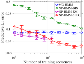
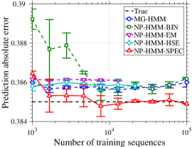
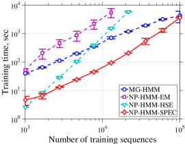
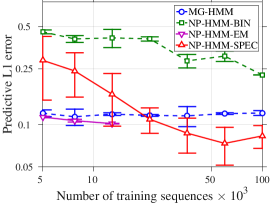
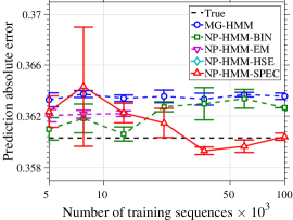
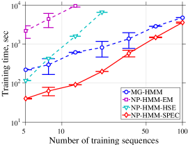
Figure 1: The upper and lower panels correspond to $m=4$ $m=8$ respectively. All figures are in log-log scale and the x-axis is the number of triples used for training. Left: $L_{1}$ error between true conditional density $p(x_{6}|x_{1:5})$, and the estimate for each method. Middle: The absolute error between the true observation and a one-step-ahead prediction. The error of the true model is denoted by a black dashed line. Right: Training time.

We compare NP-HMM-SPEC to the following. MG-HMM: An HMM trained using EM with the emissions modeled as a mixture of Gaussians. We tried $2,4$ and $8$ mixtures and report the best result. NP-HMM-BIN: A naive baseline where we bin the space into $n$ intervals and use the discrete spectral algorithm [2] with $n$ states. We tried several values for $n$ and report the best. NP-HMM-EM: The Nonparametric EM heuristic of [12]. NP-HMM-HSE: The Hilbert space embedding method of [14].

Synthetic Datasets: We first performed a series of experiments on synthetic data where the true distribution is known. The goal is to evaluate the estimated models against the true model. We generated triples from two HMMs with $m=4$ and $m=8$ states and nonparametric emissions. The details of the set up are given in Appendix E. Fig. 1 presents the results.

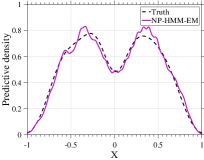
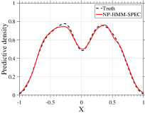
Figure 2: True and estimated one step ahead densities $p(x_{4}|x_{1:3})$ for each model. Here $m=4$ and $N=10^{4}$.

First we compare the methods on estimating the one step ahead conditional density $p(x_{6}|x_{1:5})$. We report the ${L^{1}}$ error between the true and estimated models. In Fig. 2 we visualise the estimated one step ahead conditional densities. NP-HMM-SPEC outperforms all methods on this metric. Next, we compare the methods on the prediction performance. That is, we sample sequences of length $6$ and test how well a learned model can predict $x_{6}$ conditioned on $x_{1:5}$. When comparing on squared error, the best predictor is the mean of the distribution. For all methods we use the mean of $\widehat{p}(x_{6}|x_{1:5})$ except for NP-HMM-HSE for which we used the mode since the mean cannot be computed. No method can do better than the true model (shown via the dotted line) in expectation. NP-HMM-SPEC achieves the performance of the true model with large datasets. Finally, we compare the training times of all methods. NP-HMM-SPEC is orders of magnitude faster than NP-HMM-HSE and NP-HMM-EM.

Note that the error of MG-HMM– a parametric model – stops decreasing even with large data. This is due to the bias introduced by the parametric assumption. We do not train NP-HMM-EM for longer sequences because it is too slow. A limitation of the NP-HMM-HSE method is that it cannot recover conditional probabilities – so we exclude it from that experiment. We exclude NP-HMM-BIN from the time comparison because it was much faster than all other methods. We could not include the method of [4] in our comparisons since their code was not available and their method isn’t straightforward to implement. Further, their method cannot compute joint/predictive probabilities.

Real Datasets: We compare all the above methods (except NP-HMM-EM which was too slow) on prediction error on $3$ real datasets: internet traffic [27], laser generation [28] and sleep data [29]. Each model was trained using a training sequence and then the predictions were computed on a test sequence. The details on these datasets are in Appendix E. For all methods we used the mode of the conditional distribution $p(x_{t+1}|x_{1:t})$ as the prediction as it performed better. For NP-HMM-SPEC, NP-HMM-HSE,NP-HMM-BIN we follow the procedure outlined in Section 4.3 to create triples and train with the triples. In Table 1 we report the mean prediction error and the standard error. NP-HMM-HSE and NP-HMM-SPEC perform better than the other two methods. However, NP-HMM-SPEC was faster to train (and has other attractive properties) when compared to NP-HMM-HSE.

Dataset	MG-HMM	NP-HMM-BIN	NP-HMM-HSE	NP-HMM-SPEC
Internet Traffic	$0.143\pm 0.001$	$0.188\pm 0.004$	$0.0282\pm 0.0003$	$\bf 0.016\pm 0.0002$
Laser Gen	$0.33\pm 0.018$	$0.31\pm 0.017$	$0.19\pm 0.012$	$\bf 0.15\pm 0.018$
Patient Sleep	$0.330\pm 0.002$	$0.38\pm 0.011$	$\bf 0.197\pm 0.001$	$0.225\pm 0.001$

Table 1: The mean prediction error and the standard error on the $3$ real datasets.

7 Conclusion

We proposed and studied a method for estimating the observable representation of a Hidden Markov Model whose emission probabilities are smooth nonparametric densities. We derive a bound on the sample complexity for our method. While our algorithm is similar to existing methods for discrete models, many of the ideas that generalise it to the nonparametric setting are new. In comparison to other methods, the proposed approach has some desirable characteristics: we can recover the joint/conditional densities, our theoretical results are in terms of more interpretable metrics, the method outperforms baselines and is orders of magnitude faster to train.

In this exposition only focused on one dimensional observations. The multidimensional case is handled by extending the above ideas and technology to multivariate functions. Our algorithm and the analysis carry through to the $d$-dimensional setting, mutatis mutandis. The concern however, is more practical. While we have the technology to perform various c/q-matrix operations for $d=1$ using Chebyshev polynomials, this is not yet the case for $d>1$. Developing efficient procedures for these operations in the high dimensional settings is a challenge for the numerical analysis community and is beyond the scope of this paper. That said, some recent advances in this direction are promising [30, 8].

While our method has focused on HMMs, the ideas in this paper apply for a much broader class of problems. Recent advances in spectral methods for estimating parametric predictive state representations [31], mixture models [3] and other latent variable models [32] can be generalised to the nonparamatric setting using our ideas. Going forward, we wish to focus on such models.

Acknowledgements

The authors would like to thank Alex Townsend, Arthur Gretton, and Ahmed Hefny for the helpful discussions.

Appendix A A Quart-sized Review of Continuous Linear Algebra

In this section we introduce continuous analogues of matrices and their factorisations. We only provide a brief quart-sized review for what is needed in this exposition. Chapters 3 and 4 of Townsend [6] contains a reservoir-sized review.

A matrix $F\in\mathbb{R}^{m\times n}$ is an $m\times n$ array of numbers where $F(i,j)$ denotes the entry in row $i$, column $j$. We will also look at cases where either $m$ or $n$ is infinite. A column qmatrix (quasi-matrix) $Q\in\mathbb{R}^{[a,b]\times m}$ is a collection of $m$ functions defined on $[a,b]$ where the row index is continuous and column index is discrete. Writing $Q=[q_{1},\dots,q_{m}]$ where $q_{j}:[a,b]\rightarrow\mathbb{R}$ is the $j$${}^{\textrm{th}}$ function, $Q(y,j)=q_{j}(y)$ denotes the value of the $j$${}^{\textrm{th}}$ function at $y\in[a,b]$. $Q^{\top}\in\mathbb{R}^{m\times[a,b]}$ denotes a row qmatrix with $Q^{\top}(j,y)=Q(y,j)$. A cmatrix (continous-matrix) $C\in\mathbb{R}^{[a,b]\times[c,d]}$ is a two dimensional function where both the row and column indices are continuous and $C(y,x)$ is value of the function at $(y,x)\in[a,b]\times[c,d]$. $C^{\top}\in\mathbb{R}^{[c,d]\times[a,b]}$ denotes its transpose with $C^{\top}(x,y)=C(y,x)$.

Qmatrices and cmatrices permit all matrix multiplications with suitably defined inner products. Let $F\in\mathbb{R}^{m\times n}$, $Q\in\mathbb{R}^{[a,b]\times m}$, $P\in\mathbb{R}^{[a,b]\times n}$, $R\in\mathbb{R}^{[c,d]\times m}$ and $C\in\mathbb{R}^{[a,b]\times[c,d]}$. It follows that $F(:,j)\in\mathbb{R}^{m}$, $Q(y,:)\in\mathbb{R}^{1\times m}$, $Q(:,i)\in\mathbb{R}^{[a,b]}$, $C(y,:)\in\mathbb{R}^{1\times[c,d]}$ etc. Then the following hold:

• $QF=S\in\mathbb{R}^{[a,b]\times n}\quad$ where $\quad S(y,j)=Q(y,:)F(:,j)=\sum_{k=1}^{m}Q(y,k)F(i,k)$.

• $Q^{\top}P=H\in\mathbb{R}^{m\times n}\quad$ where $\quad H(i,j)=Q(:,j)^{\top}P(:,j)=\int_{a}^{b}Q^{\top}(i,s)P(s,j)\mathrm{d}s$.

• $QR^{\top}=D\in\mathbb{R}^{[a,b]\times[c,d]}\quad$ where $\quad D(y,x)=Q(y,:)R(x,:)^{\top}=\sum_{1}^{m}Q(y,k)R^{\top}(k,x)$.

• $CR=T\in\mathbb{R}^{[a,b]\times m}\quad$ where $\quad T(y,j)=C(y,:)R(:,j)=\int_{c}^{d}C(y,s)R(s,j)\mathrm{d}s$.

Here, the integrals are with respect to the Lebesgue measure.

A cmatrix has a singular value decomposition (SVD). If $C\in\mathbb{R}^{[a,b]\times[c,d]}$, an SVD of $C$ is the sum $C(y,x)=\sum_{j=1}^{\infty}\sigma_{j}u_{j}(y)v_{j}(x),$ which converges in ${L^{2}}$. Here $\sigma_{1}\geq\sigma_{2}\geq\dots$. are the singular values of $C$. $\{u_{j}\}_{j\geq 1}$ and $\{v_{j}\}_{j\geq 1}$ are the left and right singular vectors and form orthonormal bases for ${L^{2}}([a,b])$ and ${L^{2}}([c,d])$ respectively, i.e. $\int_{a}^{b}u_{j}(s)u_{k}(s)\mathrm{d}s=\mathbbm{1}(j=k)$. It is known that the SVD of a cmatrix exists uniquely with $\sigma_{j}\rightarrow 0$, and continuous singular vectors (Theorem 3.2, [6]). Further, if $C$ is Lipshcitz continuous w.r.t both variables then the SVD is absolutely and uniformly convergent. Writing the singular vectors as infinite qmatrices $U=[u_{1},u_{2}\dots],V=[v_{1},v_{2}\dots]$, and $\Sigma={\rm diag}(\sigma_{1},\sigma_{2}\dots)$ we can write the SVD as,

$$C=U\Sigma V^{\top}=\sum_{j=1}^{\infty}\sigma_{j}U(:,j)V(:,j)^{\top}.$$

If only $m<\infty$ singular values are nonzero then we say that $C$ is of rank $m$. The SVD of a Qmatrix $Q\in\mathbb{R}^{[a,b]\times m}$ is, $Q=U\Sigma V^{\top}=\sum_{j=1}^{m}\sigma_{j}U(:,j)V(:,j)^{\top},$ where $U\in\mathbb{R}^{[a,b]\times m}$ and $V\in\mathbb{R}^{m\times m}$ have orthonormal columns and $\Sigma={\rm diag}(\sigma_{1},\dots,\sigma_{m})$ with $\sigma_{1}\geq\sigma_{2}\geq\dots\geq\sigma_{m}\geq 0$. The SVD of a qmatrix also exists uniquely (Theorem 4.1, [6]). The rank of a column qmatrix is the number of linearly independent columns (i.e. functions) and is equal to the number of nonzero singular values.

Finally, the pseudo inverse of the cmatrix $C$ is $C^{\dagger}=V\Sigma^{-1}U^{\top}$ with $\Sigma^{-1}={\rm diag}(1/\sigma_{1},1/\sigma_{2},\dots)$. The $p$-operator norm of a cmatrix, for $1\leq p\leq\infty$ is $\|C\|_{p}=\sup_{\|x\|_{p}=1}\|Cx\|_{p}$ where $x\in\mathbb{R}^{[c,d]}$, $Cx\in\mathbb{R}^{[a,b]}$, $\|x\|^{p}_{p}=\int_{c}^{d}(x(s))^{p}\mathrm{d}s$ for $p<\infty$ and $\|x\|_{\infty}=\sup_{s\in[c,d]}x(s)$. The Frobenius norm of a cmatrix is $\|C\|_{F}=\left(\int_{a}^{b}\int_{c}^{d}C(y,x)^{2}\mathrm{d}x\mathrm{d}y\right)^{1/2}$. It can be shown that $\|C\|_{2}=\sigma_{1}$ and $\|C\|^{2}_{F}=\sum_{j}\sigma_{j}^{2}$ where $\sigma_{1}\geq\sigma_{2}\geq\dots$ are its singular values. Note that analogous relationships hold with finite matrices. The pseudo inverse and norms of a qmatrix are similarly defined and similar relationships hold with its singular values.

Notation: In what follows we will use ${\bf 1}_{[a,b]}$ to denote the function taking value $1$ everywhere in $[a,b]$ and ${\bf 1}_{m}$ to denote $m$-vectors of $1$’s. When we are dealing with $L^{p}$ norms of a function we will explicitly use the subscript $L^{p}$ to avoid confusion with the operator/Frobenius norms of qmatrices and cmatrices. For example, for a cmatrix $\|C\|^{2}_{{L^{2}}}=\int\int C(\cdot,\cdot)^{2}=\|C\|^{2}_{F}$. As we have already done, throughout the paper we will overload notation for inner products, multiplications and pseudo-inverses depending on whether they hold for matrices, qmatrices or cmatrices. E.g. when $p,q\in\mathbb{R}^{m},p^{\top}q=\sum_{1}^{m}p_{i}q_{i}$ and when $p,q\in\mathbb{R}^{[a,b]}$, $p^{\top}q=\int_{a}^{b}p(s)q(s)\mathrm{d}s$. $\mathbb{P}$ will be used to denote probabilities of events while $p$ will denote probability density functions (pdf).

Appendix B Some Perturbation Theory Results for Continuous Linear Algebra

We recommend that readers unfamiliar with continuous linear algebra first read the review in Appendix A. Throughout this section $\mathcal{L}(\cdot)$ maps a matrix (including q/cmatrices) to its eigenvalues. Similarly, $\sigma(\cdot)$ maps a matrix to its singular values. When we are dealing with infinite sequences and qmatrices “=" refers to convergence in ${L^{2}}$. When dealing with infinite sequences and cmatrices, “=" refers to convergence in the operator norm. For all theorems, we follow the template of Stewart and Sun [26] for the matrix case and hence try to stick with their notation.

Before we proceed, we introduce the “cmatrix" $I_{[0,1]}$ on $[0,1]$. For any $u\in\mathbb{R}^{[0,1]}$ this is the operator which satisfies $I_{[0,1]}u=u$. That is, $(I_{[0,1]}u)(y)=\int_{0}^{1}I_{[0,1]}(y,x)u(x)\mathrm{d}x=u(y)$. Intuitively, it can be thought of as the Dirac delta function along the diagonal, $\delta(x-y)$. Let $Q=[q_{1},q_{2},\dots,]\in\mathbb{R}^{[0,1]\times\infty}$ be a qmatrix containing an orthonormal basis for $[0,1]$ and $Q_{k}\in\mathbb{R}^{[0,1]\times k}$ denote the first $k$ columns of $Q$. We make note of the following observation.

Theorem 8.

$Q_{k}Q_{k}^{\top}\rightarrow I_{[0,1]}$ as $k\rightarrow\infty$. Here convergence is in the operator norm.

Proof.

We need to show that for all $x\in\mathbb{R}^{[0,1]}$, $\|Q_{k}Q_{k}^{\top}x-x\|_{2}\rightarrow 0$. Let $x=Q\bm{\alpha}=\sum_{k=1}^{\infty}\alpha_{k}q_{k}$ be the representation of $x$ in the $Q$-basis. Here $\bm{\alpha}=(\alpha_{1},\alpha_{2},\dots)$ satisfies $\sum_{k}\alpha_{k}^{2}<\infty$. We then have $\|Q_{k}Q_{k}^{\top}x-x\|_{2}^{2}=\sum_{j=k+1}^{\infty}\alpha_{j}^{2}\rightarrow 0$ by the properties of sequences in $\ell^{2}$. ∎

We now proceed to our main theorems. We begin with a series of intermediary results.

Theorem 9.

Let $X\in\mathbb{R}^{[0,1]\times m}$. Define the linear operator ${\bf T}(X)=AX-XB$ where $A\in\mathbb{R}^{[0,1]\times[0,1]}$ and $B\in\mathbb{R}^{m\times m}$ are a square cmatrix and matrix, respectively. Then, $T$ is nonsingular if and only if $\mathcal{L}(A)\cap\mathcal{L}(B)=\varnothing$.

Proof.

Assume $\lambda\in\mathcal{L}(A)\cup\mathcal{L}(B)$. Then, let $Ap=\lambda p$, $q^{\top}B=\lambda q^{\top}$ where $p\in\mathbb{R}^{[0,1]}$ and $q\in\mathbb{R}^{m}$. Then ${\bf T}(pq^{\top})={\bf 0}$ and ${\bf T}$ is singular. This proves one side of the theorem.

Now, assume that $\mathcal{L}(A)\cap\mathcal{L}(B)=\varnothing$. As the operator is linear, it is sufficient to show that $AX-XB=C$ has a unique solution for any $C\in\mathbb{R}^{[0,1]\times m}$. Let the Schur decomposition of $B$ be $Q=V^{\top}BV$ where $V$ is orthogonal and $Q$ is upper triangular. Writing $Y=XV$ and $D=CV$ it is sufficient to show that $AY-YQ=D$ has a unique solution. We write

$$Y=(y_{1},y_{2},\dots y_{m})\in\mathbb{R}^{[0,1]\times m}\text{ and }D=(d_{1},d_{2},\dots,d_{m})\in\mathbb{R}^{[0,1]\times m}$$

and use an inductive argument over the columns of $Y$.

The first column of $Y$ is given by $Ay_{1}-Q_{11}y_{1}=(A-Q_{11}I_{[0,1]})y_{1}=d_{1}$. Since $Q_{11}\in\mathcal{L}(B)$ and $\mathcal{L}(A)\cap\mathcal{L}(B)$ is empty $(A-Q_{11}I_{[0,1]})$ is nonsingular. Therefore $y_{1}$ is uniquely determined by inverting the cmatrix (see Appendix A). Assume $y_{1},y_{2}\dots,y_{k-1}$ are uniquely determined. Then, the $k$${}^{\textrm{th}}$ column is given by $(A-Q_{kk}I_{[0,1]})y_{k}=d_{k}+\sum_{i=1}^{k-1}Q_{ik}y_{i}$. Again, $(A-Q_{kk}I_{[0,1]})$ is nonsingular by assumption, and hence this uniquely determines $y_{k}$. ∎

Corollary 10.

Let ${\bf T}$ be as defined in Theorem 9. Then

$$\mathcal{L}({\bf T})=\mathcal{L}(A)-\mathcal{L}(B)=\{\alpha-\beta:\alpha\in\mathcal{L}(A),\beta\in\mathcal{L}(B)\}.$$

Proof.

If $\lambda\in\mathcal{L}({\bf T})$ there exists $X$ such that $(A-\lambda I_{[0,1]})X-XB={\bf 0}$. Therefore, by Theorem 9 there exists $\alpha\in\mathcal{L}(A)$ and $\beta\in\mathcal{L}(B)$ such that $\lambda=\alpha-\beta$. Therefore, $\mathcal{L}({\bf T})\subset\mathcal{L}(A)-\mathcal{L}(B)$.

Conversely, consider any $\alpha\in\mathcal{L}(A)$ and $\beta\in\mathcal{L}(B)$. Then there exists $a\in\mathbb{R}^{[0,1]}$, $b\in\mathbb{R}^{m}$ such that $Aa=\alpha a$ and $b^{\top}B=\beta b^{\top}$. Writing $X=ab^{\top}$ we have $AX-XB=(\alpha-\beta)ab^{\top}$. Therefore, $\mathcal{L}(A)-\mathcal{L}(B)\subset\mathcal{L}({\bf T})$. ∎

Theorem 11.

Let ${\bf T}$ be as defined in Theorem 9. Then

$$\inf_{\|X\|_{\rm F}=1}\|{\bf T}(X)\|_{\rm F}=\min\mathcal{L}({\bf T})=\min|\mathcal{L}(A)-\mathcal{L}(B)|.$$ (7)

Proof.

For any qmatrix $P=(p_{1},p_{2},\dots,p_{m})\in\mathbb{R}^{[0,1]\times m}$ let ${\rm vec}(P)=[p_{1}^{\top},p_{2}^{\top},\dots,p_{m}^{\top}]^{\top}\in\mathbb{R}^{[0,m]\times 1}$ be the concatenation of all functions. Then ${\rm vec}(XB)=\vec{B}{\rm vec}(X)$ where,

$$\vec{B}=\begin{bmatrix}B_{11}I_{[0,1]}&B_{21}I_{[0,1]}&\cdots&B_{m1}I_{[0,1]}\\ B_{12}I_{[0,1]}&B_{22}I_{[0,1]}&\cdots&B_{m2}I_{[0,1]}\\ \vdots&\vdots&\ddots&\vdots\\ B_{1m}I_{[0,1]}&B_{2m}I_{[0,1]}&\cdots&B_{mm}I_{[0,1]}\end{bmatrix}\in\mathbb{R}^{[0,m]\times[0,m]}.$$

Here $I_{[0,1]}$ have been translated and should be interpreted as being a dirac delta function on that block. Similarly, ${\rm vec}(AX)=\vec{A}{\rm vec}(X)$ where $\vec{A}={\rm diag}(A,A,\dots,A)\in\mathbb{R}^{[0,m]\times[0,m]}$. Therefore ${\rm vec}({\bf T}(X))=(\vec{A}-\vec{B})\vec{X}$. Now noting that $\|X\|_{\rm F}=\|{\rm vec}(X)\|_{2}$ we have,

$$\inf_{\|X\|_{\rm F}=1}\|{\bf T}(X)\|_{\rm F}=\inf_{\|{\rm vec}(X)\|_{2}=1}\|{\rm vec}({\bf T}(X))\|_{2}=\min|\mathcal{L}(\vec{A}-\vec{B})|.$$

The theorem follows by noting that the eigenvalues of $(\vec{A}-\vec{B})$ are the same as those of $\mathcal{L}({\bf T})$. ∎

Theorem 12.

Let $X_{1},Y_{1}\in\mathbb{R}^{[0,1]\times\ell}$ have orthonormal columns. Then, there exist $Q\in\mathbb{R}^{\infty\times[0,1]}$ and $U_{11},V_{11}\in\mathbb{R}^{\ell\times\ell}$ such that the following holds,

$$QX_{1}U_{11}=\begin{bmatrix}I_{\ell}\\ {\bf 0}\end{bmatrix}\;\in\mathbb{R}^{\infty\times\ell},\hskip 28.90755ptQY_{1}V_{11}=\begin{bmatrix}\Gamma\\ \Sigma\\ {\bf 0}\end{bmatrix}\;\in\mathbb{R}^{\infty\times\ell}.$$

Here $\Gamma={\rm diag}(\gamma_{1},\dots,\gamma_{\ell})$, $\Sigma={\rm diag}(\sigma_{1},\dots,\sigma_{\ell})$ and they satisfy

$$0\leq\gamma_{1}\leq\dots\leq\gamma_{\ell},\,\sigma_{1}\geq\dots\geq\sigma_{\ell}\geq 0,\,\text{and}\ \gamma_{i}^{2}+\sigma_{i}^{2}=1,\,i=1,\dots,\ell.$$

Proof.

Let $X_{2},Y_{2}\in\mathbb{R}^{[0,1]\times\infty}$ be orthonormal bases for the complementary subspaces of $\mathcal{R}(X_{1}),\mathcal{R}(Y_{1})$, respectively. Denote $X=[X_{1},X_{2}]$, $Y=[Y_{1},Y_{2}]$ and

$$W=X^{\top}Y=\begin{pmatrix}W_{11}&W_{12}\\ W_{21}&W_{22}\end{pmatrix}\in\mathbb{R}^{\infty\times\infty},$$

where $W_{11}=X_{1}^{\top}Y_{1}\in\mathbb{R}^{\ell\times\ell}$ and the rest are defined accordingly. Now, using Theorem 5.1 from [26] there exist orthogonal matrices $U={\rm diag}(U_{11},U_{22}),V={\rm diag}(V_{11},V_{22})$ where $U_{11},V_{11}\in\mathbb{R}^{\ell\times\ell}$ and $U_{22},V_{22}\in\mathbb{R}^{\infty\times\infty}$ such that the following holds,

$$U^{\top}WV=\begin{pmatrix}\Gamma&-\Sigma&{\bf 0}\\ \Sigma&\Gamma&{\bf 0}\\ {\bf 0}&{\bf 0}&I_{\infty}\end{pmatrix}\in\mathbb{R}^{\infty\times\infty}.$$

Here $\Gamma,\Sigma$ satisfy the conditions of the theorem. Now set $\;\widehat{X}=[\widehat{X}_{1},\widehat{X}_{2}]$, $\;\widehat{Y}=[\widehat{Y}_{1},\widehat{Y}_{2}]$ where $\;\widehat{X}_{1}=X_{1}U_{11}$, $\;\widehat{X}_{2}=X_{2}U_{11}$, $\;\widehat{Y}_{1}=Y_{1}V_{11}$, $\;\widehat{Y}_{2}=Y_{2}V_{11}$. Then, $\widehat{X}^{\top}Y=U^{\top}WV$. Setting $Q=\widehat{X}^{\top}$ and setting $U_{11},V_{11}$ as above yields,

$$QX_{1}U_{11}=\begin{pmatrix}U_{11}^{\top}X_{1}^{\top}\\ U_{22}^{\top}X_{2}^{\top}\end{pmatrix}X_{1}U_{11}=\begin{bmatrix}I_{\ell}\\ {\bf 0}\end{bmatrix},\quad QY_{1}V_{11}=\begin{pmatrix}U_{11}^{\top}X_{1}^{\top}\\ U_{22}^{\top}X_{2}^{\top}\end{pmatrix}Y_{1}V_{11}=\begin{bmatrix}\Gamma\\ \Sigma\\ {\bf 0}\end{bmatrix}$$

where $U_{11}^{\top}X_{1}^{\top}Y_{1}U_{11}=\Gamma$, $U_{22}^{\top}X_{2}^{\top}Y_{1}U_{11}=[\Sigma^{\top},{\bf 0}^{\top}]^{\top}$ from the decomposition of $U^{\top}WV$. ∎

Remark 13.

Stewart and Sun [26] prove Theorem 5.1 for a finite unitary $W$. However, it is straightforward to verify that the same holds if $W$ is a unitary operator on the $\ell^{2}$ sequence space, i.e., Theorem 5.1 is valid for (countably) infinite matrices.

Definition 14 (Canonical Angles).

Let $\mathcal{X},\mathcal{Y}$ be $\ell$ dimensional subspaces of the same dimension for functions on $[0,1]$ and $X_{1},Y_{1}\in\mathbb{R}^{[0,1]\times\ell}$ be orthonormal functions spanning these subspaces. Then the canonical angles between $\mathcal{X}$ and $\mathcal{Y}$ are the diagonals of the matrix $\Theta[\mathcal{X},\mathcal{Y}]\stackrel{{\scriptstyle\Delta}}{{=}}\sin^{-1}(\Sigma)$ where $\Sigma$ is from Theorem 12. It follows that $\cos\Theta[\mathcal{X},\mathcal{Y}]=\Gamma$ where $\sin$ and $\cos$ are in the usual trigonometric sense and satisfy $\cos^{2}(x)+\sin^{2}(x)=1$.

Corollary 15.

Let $\mathcal{X},\mathcal{Y},X_{1},Y_{1}$ be as in Definition 14 and $X_{2},Y_{2}$ be orthonormal functions for their complementary spaces. Then, the nonzero singular values of $X_{2}^{\top}Y_{1}$ are the sines of the nonzero canonical angles between $\mathcal{X},\mathcal{Y}$. The singular values of $X_{1}^{\top}Y_{1}$ are the cosines of the nonzero canonical angles.

Proof.

From the proof of Theorem 12,

$$X_{2}^{\top}Y_{1}=U_{22}\begin{pmatrix}\Sigma\\ {\bf 0}\end{pmatrix}U_{11}^{\top},\qquad X_{1}^{\top}Y_{1}=U_{11}\Gamma U_{11}^{\top}.$$

Since $U_{11},U_{22}$ are orthogonal, the above are the SVDs of $X_{2}^{\top}Y_{1}$ and $X_{1}^{\top}Y_{1}$. ∎

Theorem 16.

Let $\mathcal{X},\mathcal{Y}$ be $\ell$ dimensional subspaces of functions on $[0,1]$ and $X_{1},Y_{1}\in\mathbb{R}^{[0,1]\times l}$ be an orthonormal bases. Let $\sin\Theta[\mathcal{X},\mathcal{Y}]={\rm diag}(\sigma_{1},\dots,\sigma_{\ell})$. Denote $P_{\mathcal{X}}=X_{1}X_{1}^{\top}$ and $P_{\mathcal{Y}}=Y_{1}Y_{1}^{\top}$. Then, the singular values of $P_{\mathcal{X}}(I_{[0,1]}-P_{\mathcal{Y}})$ are $\sigma_{1},\sigma_{2},\dots,\sigma_{\ell},0,0,\dots$.

Proof.

By Theorem 12, there exists $Q\in\mathbb{R}^{\infty\times[0,1]}$, $U_{11},V_{11}\in\mathbb{R}^{\ell\times\ell}$, such that

$$QP_{\mathcal{X}}(I_{[0,1]}-P_{\mathcal{Y}})Q^{\top}=QX_{1}X_{1}^{\top}Q^{\top}Q(I_{[0,1]}-Y_{1}Y_{1}^{\top})Q^{\top}$$

$$\hskip 21.68121pt=(QX_{1}U_{1})(U_{1}^{\top}X_{1}^{\top}Q^{\top})(I_{[0,1]}-QY_{1}V_{11}(V_{11}^{\top}Y_{1}^{\top}Q^{\top}))=\begin{bmatrix}\Sigma\\ {\bf 0}\\ {\bf 0}\end{bmatrix}\begin{bmatrix}\Sigma&-\Gamma&{\bf 0}\end{bmatrix}$$

Here we have used $I_{[0,1]}=Q^{\top}Q$. The proof of this uses a technical argument involving the dual space of the class of operators described by cmatrices. (In the discrete matrix case this is similar to how the outer product of a complete orthonormal basis results in the identity $UU^{\top}=I$.) The last step follows from Theorem 12 and some algebra. Noting that $\begin{bmatrix}\Sigma&-\Gamma&{\bf 0}\end{bmatrix}$ has orthonormal rows, it follows that the singular values of $P_{\mathcal{X}}(I_{[0,1]}-P_{\mathcal{Y}})$ are $\Sigma$. ∎

Theorem 17.

Let $A\in\mathbb{R}^{[0,1]\times[0,1]}$ satisfy,

$$A=\begin{bmatrix}X_{1}&X_{2}\end{bmatrix}\begin{bmatrix}L_{1}&{\bf 0}\\ {\bf 0}&L_{2}\end{bmatrix}\begin{bmatrix}X_{1}^{\top}\\ X_{2}^{\top}\end{bmatrix}$$

where $X_{1}\in\mathbb{R}^{[0,1]\times\ell}$ and $[X_{1},\,X_{2}]$ is unitary. Let $Z\in\mathbb{R}^{[0,1]\times m}$ and $T=AZ-ZB$ where $B\in\mathbb{R}^{m\times m}$. Let $\delta=\min|\mathcal{L}(L_{2})-\mathcal{L}(B)|>0$. Then,

$$\big{\|}\sin\Theta[\mathcal{R}(X_{1}),\mathcal{R}(Z)]\|_{\rm F}\;\leq\;\frac{\|T\|_{\rm F}}{\delta}.$$

Proof.

First note that $X_{2}^{\top}T=L_{2}X_{2}^{\top}Z-X_{2}^{\top}ZB$. The claim follows from Theorems 11 and 15.

$$\big{\|}\sin\Theta[\mathcal{R}(X_{1}),\mathcal{R}(Z)]\|_{\rm F}\,=\,\|X_{2}^{\top}Z\|_{\rm F}\,\leq\frac{\|X_{2}^{\top}T\|_{\rm F}}{\min|\mathcal{L}(L_{2})-\mathcal{L}(B)|}\leq\frac{\|T\|_{\rm F}}{\delta}.$$

∎

Theorem 18 (Wedin’s Sine Theorem for cmatrices – Frobenius form).

Let $A,\tilde{A},E\in\mathbb{R}^{[0,1]\times[0,1]}$ with $\tilde{A}=A+E$. Let $A,\tilde{A}$ have the following conformal partitions,

$$A\,=\,\begin{bmatrix}U_{1}&U_{2}\end{bmatrix}\begin{bmatrix}\Sigma_{1}&{\bf 0}\\ {\bf 0}&\Sigma_{2}\end{bmatrix}\begin{bmatrix}V_{1}^{\top}\\ V_{2}^{\top}\end{bmatrix}\,,\hskip 28.90755pt\tilde{A}\,=\,\begin{bmatrix}\tilde{U}_{1}&\tilde{U}_{2}\end{bmatrix}\begin{bmatrix}\tilde{\Sigma}_{1}&{\bf 0}\\ {\bf 0}&\tilde{\Sigma}_{2}\end{bmatrix}\begin{bmatrix}\tilde{V}_{1}^{\top}\\ \tilde{V}_{2}^{\top}\end{bmatrix}\,.$$

where $U_{1},\tilde{U}_{1}\in\mathbb{R}^{[0,1]\times m}$, $\,V_{1},\tilde{V}_{1}\in\mathbb{R}^{[0,1]\times m}$ and $U_{2},\tilde{U}_{2}\in\mathbb{R}^{[0,1]\times\infty}$, $\,V_{2},\tilde{V}_{2}\in\mathbb{R}^{[0,1]\times\infty}$. Let $R=A\tilde{V}_{1}-\tilde{U}_{1}\tilde{\Sigma}_{1}\in\mathbb{R}^{[0,1]\times m}$ and $S=A^{\top}\tilde{U}_{1}-\tilde{V}_{1}\tilde{\Sigma}_{1}\in\mathbb{R}^{[0,1]\times m}$. Assume there exists $\delta>0$ such that, $\min|\sigma(\tilde{\Sigma}_{1})-\sigma(\Sigma_{2})|\geq\delta$ and $\min|\sigma(\tilde{\Sigma}_{1})|\geq\delta$. Let $\Phi_{1},\Phi_{2}$ denote the canonical angles between $(\mathcal{R}(U_{1}),\mathcal{R}(\tilde{U}_{1}))$ and $(\mathcal{R}(V_{1}),\mathcal{R}(\tilde{V}_{1}))$ respectively. Then,

$$\sqrt{\|\sin\Phi_{1}\|^{2}_{\rm F}+\|\sin\Phi_{2}\|^{2}_{\rm F}}\;\leq\;\frac{\sqrt{\vphantom{\big{(}}\|R\|_{\rm F}^{2}+\|S\|^{2}_{\rm F}}}{\delta}.$$

Remark 19.

The two conditions on $\delta$ are needed because the theorem doesn’t require $\Sigma_{1},\Sigma_{2},\tilde{\Sigma}_{1},\tilde{\Sigma}_{2}$ to be ordered. If they were ordered, then it reduces to $\delta=\min|\sigma(\tilde{\Sigma}_{1})-\sigma(\Sigma_{2})|>0$.

Proof.

First define $Q\in\mathbb{R}^{[0,2]\times[0,2]}$,

$$Q=\begin{bmatrix}{\bf 0}&A\\ A^{\top}&{\bf 0}\end{bmatrix}.$$

It can be verified that if $u_{i}\in\mathbb{R}^{[0,1]},v_{i}\in\mathbb{R}^{[0,1]}$ are a left/right singular vector pair with singular value $\sigma_{i}$, then $(u_{i},v_{i})\in\mathbb{R}^{[0,2]}$ is an eigenvector with eigenvalue $\sigma_{i}$ and $(u_{i},-v_{i})\in\mathbb{R}^{[0,2]}$ is an eigenvector with eigenvalue $-\sigma_{i}$. Writing,

$$X=\frac{1}{\sqrt{2}}\begin{pmatrix}U_{1}&U_{1}\\ V_{1}&-V_{1}\end{pmatrix},\hskip 21.68121ptY=\frac{1}{\sqrt{2}}\begin{pmatrix}U_{2}&U_{2}\\ V_{2}&-V_{2}\end{pmatrix},$$

we have,

$$Q=\begin{bmatrix}X&Y\end{bmatrix}\begin{bmatrix}\Sigma_{1}&{\bf 0}&{\bf 0}&{\bf 0}\\ {\bf 0}&-\Sigma_{1}&{\bf 0}&{\bf 0}\\ {\bf 0}&{\bf 0}&\Sigma_{2}&{\bf 0}\\ {\bf 0}&{\bf 0}&{\bf 0}&-\Sigma_{2}\end{bmatrix}\begin{bmatrix}X^{\top}\\ Y^{\top}\end{bmatrix}.$$

We similarly define $\tilde{Q},\tilde{X},\tilde{Y}$ for $\tilde{A}$. Now let $T=Q\tilde{X}-\tilde{X}{\rm diag}(\tilde{\Sigma}_{1},-\tilde{\Sigma}_{1})$. We will apply Theorem 17 with $L_{1}={\rm diag}(\Sigma_{1},-\Sigma_{1})$, $L_{2}={\rm diag}(\Sigma_{2},-\Sigma_{2})$, $Z=\tilde{X}$, $B={\rm diag}(\tilde{\Sigma}_{1},-\tilde{\Sigma}_{1})$. Then, using the conditions on $\delta$ gives us,

$$\big{\|}\sin\Theta[\mathcal{R}(X),\mathcal{R}(\tilde{X})]\|_{\rm F}\;\leq\;\frac{\|T\|_{\rm F}}{\delta}.$$

It is straightforward to verify that $\|T\|_{\rm F}^{2}=\|R\|^{2}_{\rm F}+\|S\|^{2}_{\rm F}$. To conclude the proof, first note that

$$XX^{\top}(I_{[0,2]}-YY^{\top})=\begin{bmatrix}(U_{1}U_{1}^{\top})(I_{[0,1]}-\tilde{U}_{1}\tilde{U}_{1}^{\top})&{\bf 0}\\ {\bf 0}&(V_{1}V_{1}^{\top})(I_{[0,1]}-\tilde{V}_{1}\tilde{V}_{1}^{\top})\end{bmatrix}$$

Now, using Theorem 16 we have $\|\sin\Theta[\mathcal{R}(X),\mathcal{R}(\tilde{X})]\|^{2}_{\rm F}=\|\sin\Phi_{1}^{2}\|^{2}_{\rm F}+\|\sin\Phi_{2}^{2}\|^{2}_{\rm F}$. ∎

We can now prove Lemma 6 which follows directly from Theorem 18.

Proof of Lemma 6.

Let $\tilde{U}_{\perp}\in\mathbb{R}^{[0,1]\times m}$ be an orthonormal basis for the complementary subspace of $\mathcal{R}(\tilde{U})$. Then, by Corollary 15, $\|\tilde{U}_{\perp}^{\top}U\|_{\rm F}^{2}=\|\sin\Theta[\mathcal{R}(\tilde{U}),\mathcal{R}(U)]\|^{2}_{\rm F}$, $\|\tilde{V}_{\perp}^{\top}V\|_{\rm F}^{2}=\|\sin\Theta[\mathcal{R}(\tilde{V}),\mathcal{R}(V)]\|^{2}_{\rm F}$. For $R,S$ as defined in Theorem 18, we have. $\|R\|^{2}_{\rm F},\|S\|^{2}_{\rm F}<\|E\|^{2}_{\rm F}$. The lemma follows via the $\sin$–$\cos$ relationships for canonical angles,

$$\min\sigma(\tilde{U}^{\top}U)^{2}=1-\max\sigma(\tilde{U}_{\perp}^{\top}U)^{2}\geq 1-\|\tilde{U}_{\perp}^{\top}U\|_{\rm F}^{2}\geq 1-\frac{2\|E\|^{2}_{\rm F}}{\delta^{2}}.$$

where $\delta=\sigma_{m}(A)$. ∎

Next we prove the pseudo-inverse theorem. Recall that for $A\in\mathbb{R}^{[0,1]\times m}$ the SVD is $A=U\Sigma V^{\top}$ where $U\in\mathbb{R}^{[0,1]\times m}$, $\Sigma\in\mathbb{R}^{m\times m}$ and $V\in\mathbb{R}^{m\times m}$ where $U,V$ have orthonormal columns. Denote its pseudo-inverse by $A^{\dagger}=V\Sigma^{-1}U^{\top}$.

Proof of Lemma 7.

Let $A=U\Sigma V$ be the SVD of $A$ and $\tilde{A}=\tilde{U}\tilde{\Sigma}\tilde{V}$ be the SVD of $\tilde{A}$. Let $\widetilde{P}=\tilde{U}\tilde{U}^{\top}$, $R=VV^{\top}$, $\widetilde{R}=\tilde{V}\tilde{V}^{\top}$, $P_{\perp}=I_{[0,1]}-UU^{\top}$, $\widetilde{R}_{\perp}=I_{[0,1]}-\tilde{V}\tilde{V}^{\top}$ and $P=UU^{\top}$. We then have,

$$\tilde{A}^{\dagger}-A^{\dagger}\; =\;\;-\tilde{A}^{\dagger}\widetilde{P}ERA^{\dagger}\,+\,(\tilde{A}^{\top}\tilde{A})^{\dagger}\widetilde{R}E^{\top}P_{\perp}\,+\,\widetilde{R}_{\perp}EP(AA^{\top})^{\dagger}$$

$$\|\tilde{A}^{\dagger}-A^{\dagger}\|_{2}\; \leq\;\;\|\tilde{A}^{\dagger}\|_{2}\|E\|_{2}\|A^{\dagger}\|_{2}\,+\,\|(\tilde{A}^{\top}\tilde{A})^{\dagger}\|_{2}\|E\|_{2}\,+\,\|E\|_{2}\|(AA^{\top})^{\dagger}\|_{2}$$

$$=\;\;\left(\|\tilde{A}^{\dagger}\|_{2}\|A^{\dagger}\|_{2}+\|\tilde{A}^{\dagger}\|_{2}^{2}+\|A^{\dagger}\|_{2}^{2}\right)\|E\|_{2}\;\leq\;3\max\{\|\tilde{A}\|_{2}^{2},\|A\|_{2}^{2}\}\|E\|_{2}$$

The first step is obtained by substitutine for $\widetilde{P},E,R,\widetilde{R},P_{\perp},\widetilde{R}_{\perp}$ and $P$, the second step uses the triangle inequality, and the third step uses $\tilde{A}^{\top}\tilde{A}=U\Sigma^{2}U^{\top}$, $AA^{\top}=V\Sigma^{2}V^{\top}$. ∎

Remark 20.

$P,\widetilde{P},R,\widetilde{R}$ can be shown to be the projection operators to $\mathcal{R}(A)$, $\mathcal{R}(\tilde{A})$, $\mathcal{R}(A^{\top})$ and $\mathcal{R}(\tilde{A}^{\top})$. Here, $\mathcal{R}(A)=\{Ax;x\in\mathbb{R}^{m}\}\subset\mathbb{R}^{[0,1]}$ is the range of $A$. $\mathcal{R}(\tilde{A})\subset\mathbb{R}^{[0,1]}$, $\mathcal{R}(A^{\top})\subset\mathbb{R}^{m}$ and $\mathcal{R}(\tilde{A}^{\top})\subset\mathbb{R}^{m}$ are defined similarly. $P_{\perp}$, $\widetilde{R}_{\perp}$ are the complementary projectors of $P,\widetilde{R}$.

Finally, we state an analogue of Weyl’s theorem for cmatrices which bounds the difference in the singular values in terms of the operator norm of the perturbation. While Weyl’s theorem has been studied for general operators [23], we use the form below from Townsend [6] for cmatrices.

Lemma 21 (Weyl’s Theorem for Cmatrices, [6].).

Let $A,E\in\mathbb{R}^{[a,b]\times[c,d]}$ and $\tilde{A}=A+E$. Let the singular values of $A$ be $\sigma_{1}\geq\sigma_{2},\dots$ and those of $\tilde{A}$ be $\tilde{\sigma}_{1}\geq\tilde{\sigma}_{2},\dots$. Then,

$$|\sigma_{i}-\tilde{\sigma}_{i}|\leq\|E\|_{2}\quad\forall i\geq 1.$$

Appendix C Concentration of Kernel Density Estimation

We will first define the Hölder class in high dimensions.

Definition 22.

Let $\mathcal{X}\subset\mathbb{R}^{d}$ be a compact space. For any $r=(r_{1},\dots,r_{d})$, $r_{i}\in\mathbb{N}$, let $|r|=\sum_{i}r_{i}$ and $D^{r}=\frac{\partial^{|r|}}{\partial x_{1}^{r_{1}}\dots x_{d}^{r_{d}}}$. The Hölder class $\mathcal{H}_{d}(\beta,L)$ is the set of functions of $L_{2}(\mathcal{X})$ satisfying

$$|D^{r}f(x)-D^{r}f(y)|\leq L\|x-y\|^{\beta-|r|},$$ (8)

for all $r$ such that $|r|\leq\lfloor\beta\rfloor$ and for all $x,y\in\mathcal{X}$.

The following result establishes concentration of kernel density estimators. At a high level, we follow the standard KDE analysis techniques to decompose the ${L^{2}}$ error into bias and variance terms and bound them separately. A similar result for 2-dimensional densities was given by Liu et al. [24]. Unlike the previous work, here we deal with the general $d$-dimensional case as well as explicitly delineate the dependencies of the concentration bounds on the deviation, $\varepsilon$.

Lemma 23.

Let $f\in\mathcal{H}_{d}(\beta,L)$ be a density on $[0,1]^{d}$ and assume we have $N$ i.i.d samples $\{X_{i}\}_{i=1}^{N}\sim f$. Let $\hat{f}$ be the kernel density estimate obtained using a kernel with order at least $\beta$ and bandwidth $h=\big{(}\frac{\log N}{N}\big{)}^{\frac{1}{2\beta+d}}$. Then there exist constants $\kappa_{1},\kappa_{2},\kappa_{3},\kappa_{4}>0$ such that for all $\varepsilon<\kappa_{4}$ and number of samples satisfying $\frac{N}{\log N}>\frac{\kappa_{1}}{\varepsilon^{2+\frac{d}{\beta}}}$ we have,

$$\mathbb{P}\left(\|\hat{f}-f\|_{L^{2}}>\varepsilon\right)\leq\kappa_{2}\exp\left(-\kappa_{3}N^{\frac{2\beta}{2\beta+d}}(\log N)^{\frac{d}{2\beta+d}}\varepsilon^{2}\right)$$ (9)

Proof.

First note that

$$\mathbb{P}\big{(}\|\hat{f}-f\|_{L^{2}}>\varepsilon\big{)}\leq\mathbb{P}\big{(}\|\hat{f}-\mathbb{E}\hat{f}\|_{L^{2}}+\|\mathbb{E}\hat{f}-f\|_{L^{2}}>\varepsilon\big{)}.$$ (10)

Using the Hölderian conditions and assumptions on the kernel, standard techniques for analyzing the KDE [13, 17], give us a bound on the bias, $\|\mathbb{E}\hat{f}-f\|_{L^{2}}\leq\kappa_{5}h^{\beta}$, where $\kappa_{5}=L\int K(u)u^{\beta}\mathrm{d}u$. When the number of samples, $N$, satisfies

$$\frac{N}{\log N}\;>\;\left(\frac{2\kappa^{\prime}_{5}}{\varepsilon}\right)^{2+\frac{d}{\beta}}=\frac{\kappa_{5}}{\varepsilon^{2+\frac{d}{\beta}}},\,\mathrm{where}\ \kappa_{5}\stackrel{{\scriptstyle\Delta}}{{=}}(2\kappa^{\prime}_{5})^{2+\frac{d}{\beta}}$$ (11)

we have $\|\mathbb{E}\hat{f}-f\|_{L^{2}}\leq\varepsilon/2$, and hence (10) turns into $\mathbb{P}\big{(}\|\hat{f}-f\|_{L^{2}}>\varepsilon\big{)}\leq\mathbb{P}\big{(}\|\hat{f}-\mathbb{E}\hat{f}\|_{L^{2}}>\varepsilon/2\big{)}$.

The main challenge in bounding the first term is that we want the difference to hold in ${L^{2}}$. The standard techniques that bound the pointwise variance would not be sufficient here. To overcome the limitations, we use Corollary 2.2 from Giné and Guillou [25]. Using their notation we have,

$$\sigma^{2}\;\; =\;\sup_{t\in[0,1]^{d}}\mathbb{V}_{X\sim f}\left[\frac{1}{h^{d}}K\left(\frac{X-t}{h}\right)\right]$$

$$\leq\;\sup_{t\in[0,1]^{d}}\frac{1}{h^{2d}}\int K^{2}\left(\frac{x-t}{h}\right)f(x)\mathrm{d}x$$

$$=\sup_{t\in[0,1]^{d}}\frac{1}{h^{d}}\int K^{2}(u)f(t+uh)\mathrm{d}u\;\leq\;\frac{\|f\|_{\infty}\|K\|_{L^{2}}}{h^{d}}$$

$$U\;\; =\;\sup_{t\in[0,1]^{d}}\left\|\frac{1}{h^{d}}K\left(\frac{X-t}{h}\right)\right\|_{\infty}\;=\;\frac{\|K\|_{L^{\infty}}}{h^{d}}.$$

Then, there exist constants $\kappa_{2},\kappa_{3},\kappa^{\prime}_{4}$ such that for all $\varepsilon\in\left(\kappa^{\prime}_{4}\frac{\sigma}{\sqrt{n}}\sqrt{\log\frac{U}{\sigma}},\,\frac{\sigma^{2}}{U}\kappa^{\prime}_{4}\right)$ we have,

$$\mathbb{P}\left(\|\hat{f}-\mathbb{E}\hat{f}\|_{L^{2}}>\frac{\varepsilon}{2}\right)\leq\kappa_{2}\exp\left(-\kappa_{3}Nh^{d}\varepsilon^{2}\right).$$

Substituting for $h$ and then combining this with (10) gives us the probability inequality of the theorem. All that is left to do is to verify the that the conditions on $\varepsilon$ hold. The upper bound condition requires $\varepsilon\leq\frac{\kappa^{\prime}_{4}\|f\|_{\infty}\|K\|_{L^{2}}}{\|K\|_{L^{\infty}}}\stackrel{{\scriptstyle\Delta}}{{=}}\kappa_{4}$. After some algebra, the lower bound on $\varepsilon$ reduces to $\frac{N}{\log N}\;>\;\frac{\kappa_{6}}{\varepsilon^{2+\frac{d}{\beta}}}$. Combining this with the condtion (11) and taking $\kappa_{1}=\max(\kappa_{6},\kappa_{5})$ gives the theorem. ∎

In order to apply the above lemma, we need $P_{1},P_{21},P_{321}$ to satisfy the Hölder condition. The following lemma shows that if all $O_{k}$’s are Hölderian, so are $P_{1},P_{21},P_{321}$.

Lemma 24.

Assume that the observation probabilities belong to the one dimensional Hölder class; $\forall\ell\in[m],O_{\ell}\in\mathcal{H}_{1}(\beta,L)$. Then for some constants $L_{1},L_{2},L_{3}$, $P_{1}\in\mathcal{H}_{1}(\beta,L_{1})$, $P_{21}\in\mathcal{H}_{2}(\beta,L_{2})$, $P_{321}\in\mathcal{H}_{3}(\beta,L_{3})$.

Proof.

We prove the statement for $P_{21}$. The other two follow via a similar argument. Let $r=(r_{1},r_{2})$, $r_{i}\in\mathbb{N}$, $|r|=r_{1}+r_{2}\leq\beta$, and let $(s,t),(s^{\prime},t^{\prime})\in[0,1]^{d}$. Note that we can write,

$$P_{21}(s,t)=\sum_{k\in[m]}\sum_{\ell\in[m]}p(x_{2}=s,x_{1}=t,h_{2}=k,h_{1}=\ell)=\sum_{k\in[m]}\sum_{\ell\in[m]}\alpha_{kl}O_{k}(s)O_{\ell}(t),$$

where $\sum_{k,\ell}\alpha_{k\ell}=1$. Then,

$$\frac{\partial^{|r|}P_{21}(s,t)}{\partial s^{r_{1}}\partial t^{r_{2}}}-\frac{\partial^{|r|}P_{21}(s^{\prime},t^{\prime})}{\partial s^{r_{1}}\partial t^{r_{2}}}$$

$$\hskip 28.90755pt=\;\sum_{k,\ell}\alpha_{k\ell}\left(\frac{\partial O_{k}(s)}{\partial s^{r_{1}}}\frac{\partial O_{\ell}(t)}{\partial t^{r_{2}}}\,-\,\frac{\partial O_{k}(s^{\prime})}{\partial s^{r_{1}}}\frac{\partial O_{\ell}(t^{\prime})}{\partial t^{r_{2}}}\right)$$

$$\hskip 28.90755pt\leq\;\sum_{k,\ell}\alpha_{k\ell}\left(\left|\frac{\partial O_{k}(s)}{\partial s^{r_{1}}}\right|\left|\frac{\partial O_{\ell}(t)}{\partial t^{r_{2}}}-\frac{\partial O_{\ell}(t^{\prime})}{\partial t^{r_{2}}}\right|\;+\;\right.$$

$$\hskip 108.405pt\left.\left|\frac{\partial O_{\ell}(t^{\prime})}{\partial t^{r_{2}}}\right|\left|\frac{\partial O_{k}(s)}{\partial s^{r_{1}}}-\frac{\partial O_{\ell}(s^{\prime})}{\partial s^{r_{1}}}\right|\right)$$

$$\hskip 28.90755pt\leq\;\sum_{k,\ell}\alpha_{kl}\left(L^{\prime}L|t-t^{\prime}|^{\beta-r_{2}}+L^{\prime}L|s-s^{\prime}|^{\beta-r_{1}}\right) (\text{H\"{o}lder condition})$$

$$\hskip 28.90755pt\leq\;L^{\prime}L\left(|t-t^{\prime}|^{\beta-|r|}+|s-s^{\prime}|^{\beta-|r|}\right) (\text{domain of }s,s^{\prime}\text{ and }t,t^{\prime})$$

$$\hskip 28.90755pt\leq\;L_{2}\sqrt{(t-t^{\prime})^{2}+(s-s^{\prime})^{2}}^{\beta-|r|}$$

Here, the third step uses the Hölder conditions on $O_{k}$ and $O_{\ell}$ and the fact that the partial fractions are bounded in a bounded domain by a constant, which we denoted $L^{\prime}$, due to the Hölder condition. Since $r_{1}+r_{2}=|r|\leq\beta$ and $r_{1},r_{2}$ are positive integers, we have $x^{\beta-r_{i}}\leq x^{\beta-r},i=1,2$ for any $x\in[0,1]$, which implies the fourth step. The last step uses Jensen’s inequality and sets $L_{2}\equiv L^{\prime}L$. ∎

The corollary belows follws as a direct consequence of Lemmas 23 and 24. We have absorbed the constants $L_{1},L_{2},L_{3}$ into $\kappa_{1},\kappa_{2},\kappa_{3},\kappa_{4}$.

Corollary 25.

Assume the HMM satisfies the conditions given in Section 3. Let $\epsilon_{1},\epsilon_{21},\epsilon_{321}\in(0,\kappa_{4})$ and $\eta\in(0,1)$. If the number of samples $N$ is large enough such that the following are true,

$$\frac{N}{\log N}\,>\,\frac{\kappa_{1}}{\epsilon_{1}^{2+\frac{1}{\beta}}}\;,\hskip 36.135pt\frac{N}{\log N}\,>\,\frac{\kappa_{1}}{\epsilon_{21}^{2+\frac{2}{\beta}}}\;,\hskip 36.135pt\frac{N}{\log N}\,>\,\frac{\kappa_{1}}{\epsilon_{321}^{2+\frac{3}{\beta}}}\;,$$

$$N(\log N)^{\frac{1}{2\beta}}\,>\,\frac{1}{\epsilon_{1}^{2+\frac{1}{\beta}}}\left(\frac{1}{\kappa_{3}}\log\left(\frac{3\kappa_{2}}{\eta}\right)\right)^{1+\frac{1}{2\beta}}$$

$$N(\log N)^{\frac{2}{2\beta}}\,>\,\frac{1}{\epsilon_{21}^{2+\frac{2}{\beta}}}\left(\frac{1}{\kappa_{3}}\log\left(\frac{3\kappa_{2}}{\eta}\right)\right)^{1+\frac{2}{2\beta}}$$

$$N(\log N)^{\frac{3}{2\beta}}\,>\,\frac{1}{\epsilon_{321}^{2+\frac{3}{\beta}}}\left(\frac{1}{\kappa_{3}}\log\left(\frac{3\kappa_{2}}{\eta}\right)\right)^{1+\frac{3}{2\beta}}$$

then with at least $1-\eta$ probability the ${L^{2}}$ errors between $P_{1},P_{21},P_{321}$ and the KDE estimates $\widehat{P}_{1},\widehat{P}_{21},\widehat{P}_{321}$ satisfy,

$$\|P_{1}-\widehat{P}_{1}\|_{L^{2}}\leq\epsilon_{1},\hskip 21.68121pt\|P_{21}-\widehat{P}_{21}\|_{L^{2}}\leq\epsilon_{21},\hskip 21.68121pt\|P_{321}-\widehat{P}_{321}\|_{L^{2}}\leq\epsilon_{321}.$$

Appendix D Analysis of the Spectral Algorithm

Our proof is a brute force generalization of the analysis in Hsu et al. [2]. Following their template, we use establish a few technical lemmas. We mainly focus on the cases where our analysis is different.

Throughout this section $\epsilon_{1},\epsilon_{21},\epsilon_{321}$ will refer to ${L^{2}}$ errors. Using our notation for c/q-matrices the errors can be written as,

$$\epsilon_{1} =\|P_{1}-\widehat{P}_{1}\|_{L^{2}}=\|P_{1}-\widehat{P}_{1}\|_{F},$$

$$\epsilon_{21} =\|P_{21}-\widehat{P}_{21}\|_{L^{2}}=\|P_{21}-\widehat{P}_{21}\|_{F},$$

$$\epsilon_{321} =\|P_{321}-\widehat{P}_{321}\|_{L^{2}}.$$

We begin with a series of Lemmas.

Lemma 26.

Let $\epsilon_{21}\leq\varepsilon\sigma_{m}(P_{21})$ where $\varepsilon<\frac{1}{1+\sqrt{2}}$. Denote $\varepsilon_{0}=\frac{\epsilon_{21}^{2}}{((1-\varepsilon)\sigma_{m}(P_{21}))^{2}}<1$. Then the following hold,

1. $\sigma_{m}(\widehat{U}^{\top}\widehat{P}_{21})\geq(1-\varepsilon)\sigma_{m}(P_{21})$.

2. $\sigma_{m}(\widehat{U}^{\top}P_{21})\geq\sqrt{1-\varepsilon_{0}}\sigma_{m}(P_{21})$.

3. $\sigma_{m}(\widehat{U}^{\top}P_{21})\geq\sqrt{1-\varepsilon_{0}}\sigma_{m}(P_{21})$.

Proof.

The proof follows Hsu et al. [2] after an application of Weyl’s theorem (Lemma 21) and Wedin’s sine theorem (Lemma 6) for cmatrices. ∎

We define an alternative observable representation for the true HMM given by, $\widetilde{b}_{\infty},\widetilde{b}_{1}\in\mathbb{R}^{m}$ and $\widetilde{B}:[0,1]\rightarrow\mathbb{R}^{m\times m}$.

$$\widetilde{b}_{1} =\widehat{U}^{\top}P_{1}=(\widehat{U}^{\top}O)\pi$$

$$\widetilde{b}_{\infty} =(P_{21}^{\top}\widehat{U})P_{1}=(\widehat{U}^{\top}O)^{-1}{\bf 1}_{m}$$

$$\widetilde{B}(x) =(\widehat{U}^{\top}P_{3x1})(\widehat{U}^{\top}P_{21})^{\dagger}=(\widehat{U}^{\top}O)A(x)(\widehat{U}^{\top}O)^{-1}.$$

As long as $\widehat{U}^{\top}O$ is invertible, the above parameters constitute a valid observable representation. This is guaranteed if $\widehat{U}$ is sufficiently close to $U$. We now define the following error terms,

$$\delta_{\infty}\; =\quad\|(\widehat{U}^{\top}O)^{\top}(\widehat{b}_{\infty}-\widetilde{b}_{\infty})\|_{\infty}=\quad\|(\widehat{U}^{\top}O)^{\top}\widehat{b}_{\infty}-{\bf 1}_{m}\|_{\infty}$$

$$\delta_{1}\; =\quad\|(\widehat{U}^{\top}O)^{-1}(\widehat{B}(x)-\widetilde{B}(x))(\widehat{U}^{\top}O)\|_{1}=\quad\|(\widehat{U}^{\top}O)^{-1}\widehat{B}(x)(\widehat{U}^{\top}O)-A(x)\|_{1}$$

$$\Delta(x)\; =\quad\|(\widehat{U}^{\top}O)^{-1}(\widehat{B}(x)-\widetilde{B}(x))\widehat{U}^{\top}O\|_{1}\;=\quad\|(\widehat{U}^{\top}O)^{-1}\widehat{B}(x)-A(x)\|_{1}$$

$$\Delta\; =\quad\int_{x\in[0,1]}\Delta(x)\mathrm{d}x$$

The next lemma bounds the above quantities in terms of $\epsilon_{1},\epsilon_{21},\epsilon_{321}$.

Lemma 27.

Assume $\epsilon_{21}<\sigma_{m}(P_{21})/3$. Then, there exists constants $c_{1},c_{2},c_{3},c_{4}$ such that,

$$\delta_{\infty} \;\leq\;\;c_{1}\;\sigma_{1}(O)\left(\frac{\epsilon_{21}}{\sigma_{m}(P_{21})^{2}}\,+\,\frac{\epsilon_{1}}{\sigma_{m}(P_{21})}\right)$$

$$\delta_{1} \;\leq\;\;c_{2}\;\frac{\epsilon_{1}}{\sigma_{m}(O)}$$

$$\Delta(x) \;\leq\;\;c_{3}\;\sqrt{m}\;\kappa(O)\left(\frac{\epsilon_{21}}{\sigma_{m}(P_{21})^{2}}\|P_{3x1}\|_{2}+\frac{\|P_{3x1}-\widehat{P}_{3x1}\|_{2}}{\sigma_{m}(P_{21})^{2}}\right)$$

$$\Delta \;\leq\;\;c_{4}\;\sqrt{m}\;\kappa(O)\left(\frac{\epsilon_{21}}{\sigma_{m}(P_{21})^{2}}+\frac{\epsilon_{321}}{\sigma_{m}(P_{21})^{2}}\right)$$

Proof.

We will use $\lesssim,\gtrsim$ to denote inequalities ignoring constants. First we bound $\delta_{\infty}\leq\|(\widehat{U}^{\top}O)^{\top}(\widehat{b}_{\infty}-\widetilde{b}_{\infty})\|_{2}\leq\sigma_{1}(O)\|\widehat{b}_{\infty}-\widetilde{b}_{\infty}\|_{2}$. Then we note,

$$\|\widehat{b}_{\infty}-\widetilde{b}_{\infty}\|_{2} \leq\|(\widehat{P}_{21}^{\top}\widehat{U})^{\dagger}\widehat{P}_{1}-(P_{21}\widehat{U})^{\dagger}P_{1}\|_{2}$$

$$\leq\|(\widehat{P}_{21}^{\top}\widehat{U})^{\dagger}-(P_{21}^{\top}\widehat{U})^{\dagger}\|_{2}\|\widehat{P}_{1}\|_{2}\;+\;\|(P_{21}^{\top}\widehat{U})^{\dagger}\|_{2}\|\widehat{P}_{21}-P_{1}\|_{2}$$

$$\lesssim\frac{\epsilon_{21}}{\min\{\sigma_{m}(\widehat{P}_{21}^{\top}),\sigma_{m}(P_{21}^{\top}\widehat{U})\}^{2}}\;+\;\frac{\epsilon_{1}}{\sigma_{m}(P_{21}^{\top}\widehat{U})}$$

$$\lesssim\frac{\epsilon_{21}}{\sigma_{m}(P_{21})^{2}}\;+\;\frac{\epsilon_{1}}{\sigma_{m}(P_{21})},$$

where the third and fourth steps use Lemma 26 and Lemma 7 (the pseudoinverse theorem for qmatrices). This establishes the first result. The second result is straightforward from Lemma 26.

$$\delta_{1}\leq\sqrt{m}\|(\widehat{U}^{\top}O)^{-1}\|_{2}\|\widehat{b}_{1}-\widetilde{b}_{1}\|_{2}\leq\sqrt{m}\frac{\|\widehat{b}_{1}-\widetilde{b}_{1}\|_{2}}{\sigma_{m}(\widehat{U}^{\top}O)}\lesssim\sqrt{m}\frac{\|\widehat{U}^{\top}(\widehat{P}_{1}-P_{1})\|_{2}}{\sigma_{m}(O)}\lesssim\frac{\sqrt{m}\epsilon_{1}}{\sigma_{m}(O)}.$$

For the third result, we first note

$$\Delta(x) \leq\sqrt{m}\|(\widehat{U}^{\top}O)^{-1}\|_{2}\|\widehat{B}(x)-\widetilde{B}(x)\|_{2}\|\widehat{U}^{\top}O\|_{2}\leq\sqrt{m}\frac{\sigma_{1}(O)}{\sigma_{m}(\widehat{U}^{\top}O)}\|\widehat{B}(x)-\widetilde{B}(x)\|_{2}$$

$$\lesssim\sqrt{m}\;\kappa(O)\|\widehat{B}(x)-\widetilde{B}(x)\|_{2}$$

To bound the last term we decompose it as follows.

$$\|\widehat{B}(x)-\widetilde{B}(x)\|_{2}\; =\;\|(\widehat{U}^{\top}P_{3x1})(\widehat{U}^{\top}P_{21})^{\dagger}-(\widehat{U}^{\top}\widehat{P}_{3x1})(\widehat{U}^{\top}\widehat{P}_{21})^{\dagger}\|_{2}$$

$$\leq\;\|(\widehat{U}^{\top}P_{3x1})((\widehat{U}^{\top}P_{21})^{\dagger}-(\widehat{U}^{\top}\widehat{P}_{21})^{\dagger})\|_{2}\;+\;\|\widehat{U}^{\top}(P_{3x1}-\widehat{P}_{3x1})(\widehat{U}^{\top}\widehat{P}_{21})^{\dagger}\|_{2}$$

$$\leq\|P_{3x1}\|_{2}\|\|(\widehat{U}^{\top}P_{21})^{\dagger}-(\widehat{U}^{\top}\widehat{P}_{21})^{\dagger}\|_{2}\;+\;\|P_{3x1}-\widehat{P}_{3x1}\|_{2}\|(\widehat{U}^{\top}\widehat{P}_{21})^{\dagger}\|_{2}$$

$$\lesssim\|P_{3x1}\|_{2}\frac{\epsilon_{21}}{\sigma_{m}(P_{21})^{2}}+\frac{\|P_{3x1}-\widehat{P}_{3x1}\|_{2}}{\sigma_{m}(P_{21})}.$$

This proves the third claim. For the last claim, we make use of the proven statements. Observe,

$$\int\|P_{3x1}\|_{2}\mathrm{d}x\;\leq\;\left(\int\|P_{3x1}\|_{2}^{2}\mathrm{d}x\right)^{1/2}\;\leq\;\left(\int\int\int P_{321}(s,x,t)^{2}\mathrm{d}s\mathrm{d}t\mathrm{d}x\right)^{1/2}=\|P_{321}\|_{L^{2}},$$

where the first step uses inclusion of the $L^{p}$ norms in $[0,1]$. The second step uses $\|\cdot\|_{2}\leq\|\cdot\|_{\rm F}$ for cmatrices. A similar argument shows $\int_{x}\|P_{3x1}-\widehat{P}_{3x1}\|_{2}\leq\epsilon_{321}$. Combining these results gives the fourth claim. ∎

Finally, we need the following Lemma. The proof almost exactly replicates the proof of Lemma 12 in Hsu et al. [2], as all operations can be done with just matrices.

Lemma 28.

Assume $\epsilon_{321}\leq\sigma_{m}(P_{21})/3$. Then $\forall t\geq 0$,

$$\int|p(x_{1:t})-\widehat{p}(x_{1:t})|\mathrm{d}x_{1:t}\;\;\leq\quad\delta_{\infty}+(1+\delta_{\infty})\left((1+\Delta)^{t}\delta_{1}+(1+\Delta)^{t}-1\right),$$ (12)

where the integral is over $[0,1]^{t}$.

We are now ready to prove Theorem 5.

Proof of Theorem 5.

If $\epsilon_{1},\epsilon_{21},\epsilon_{321}$ satisfy the following for appropriate choices of $c_{5},c_{6},c_{7}$,

$$\epsilon_{1}\;\leq\;c_{5}\min(\sigma_{m}(P_{21}),\frac{\kappa(O)}{\sqrt{m}})\epsilon,\quad\epsilon_{21}\;\leq\;c_{6}\frac{\sigma_{m}(P_{21})^{2}}{\kappa(O)}\epsilon,\quad\epsilon_{321}\;\leq\;c_{7}\frac{\sigma_{m}(P_{21})}{\sigma_{1}(O)}\frac{1}{t\sqrt{m}}\epsilon,$$ (13)

we then have $\delta_{1}\leq\epsilon/20$, $\delta_{\infty}\leq\epsilon/20$ and $\Delta\leq 0.4\epsilon/t$. Plugging these expressions into Lemma 28 gives $\int|p(x_{1:t})-\widehat{p}(x_{1:t})|\mathrm{d}x_{1:t}\leq\epsilon$. When we plug the expresssions for $\epsilon_{1},\epsilon_{21},\epsilon_{321}$ in (13) into Corollary 25 we get the required sample complexity. ∎

Appendix E Addendum to Experiments

Details on Synthetic Experiments: Figure 3 shows the emission probabilities used in our synthetic experiments. For the transition matrices, we sampled the entries of the matrix from a $U(0,1)$ distribution and then renormalised the columns to sum to $1$.

In our implementation, we use a Gaussian kernel for the KDE which is of order $\beta=2$. While higher order kernels can be constructed using Legendre polynomials [17], the Gaussian kernel was more robust in practice. The bandwidth for the kernel was chosen via cross validation on density estimation.

Figure 3: An illustration of the nonparametric emission probabilities used in our experiments.

Details on Real Datasets: Here, we first estimate the model parameters using the training sequence. Given a test sequence $x_{1:n}$, we predict $x_{t+1}$ conditioned on the previous $x_{1:t}$ for $t=1:n$.

1. Internet Traffic. Training sequence length: $10,000$. Test sequence length: $10$.

2. Laser Generation. Training sequence length: $10,000$. Test sequence length: $100$.

3. Physiological data. Training sequence length: $15,000$. Test sequence length: $100$.

References

• Rabiner [1989] Lawrence R. Rabiner. A Tutorial on Hidden Markov Models and Selected Applications in Speech Recognition. In Proceedings of the IEEE, 1989.
• Hsu et al. [2009] Daniel J. Hsu, Sham M. Kakade, and Tong Zhang. A Spectral Algorithm for Learning Hidden Markov Models. In COLT, 2009.
• Anandkumar et al. [2012] Animashree Anandkumar, Daniel Hsu, and Sham M Kakade. A Method of Moments for Mixture Models and Hidden Markov Models. arXiv preprint arXiv:1203.0683, 2012.
• Siddiqi et al. [2010] Sajid M. Siddiqi, Byron Boots, and Geoffrey J. Gordon. Reduced-Rank Hidden Markov Models. In AISTATS, 2010.
• Townsend and Trefethen [2015] Alex Townsend and Lloyd N Trefethen. Continuous analogues of matrix factorizations. In Proc. R. Soc. A, 2015.
• Townsend [2014] Alex Townsend. Computing with Functions in Two Dimensions. PhD thesis, University of Oxford, 2014.
• Driscoll et al. [2014] Tobin A Driscoll, Nicholas Hale, and Lloyd N Trefethen. Chebfun guide. Pafnuty Publ, 2014.
• Townsend, Alex and Trefethen, Lloyd N. [2013] Townsend, Alex and Trefethen, Lloyd N. An extension of chebfun to two dimensions. SIAM J. Scientific Computing, 2013.
• Littman et al. [2001] Michael L Littman, Richard S Sutton, and Satinder P Singh. Predictive representations of state. In NIPS, volume 14, pages 1555–1561, 2001.
• Dempster et al. [1977] A. P. Dempster, N. M. Laird, and D. B. Rubin. Maximum likelihood from incomplete data via the EM algorithm. JOURNAL OF THE ROYAL STATISTICAL SOCIETY, SERIES B, 1977.
• Welch [2003] Lloyd R Welch. Hidden Markov models and the Baum-Welch algorithm. IEEE Information Theory Society Newsletter, 2003.
• Benaglia et al. [2009] Tatiana Benaglia, Didier Chauveau, and David R Hunter. An EM-like algorithm for semi-and nonparametric estimation in multivariate mixtures. Journal of Computational and Graphical Statistics, 2009.
• Wasserman [2006] Larry Wasserman. All of Nonparametric Statistics. Springer-Verlag NY, 2006.
• Song et al. [2010] Le Song, Byron Boots, Sajid M Siddiqi, Geoffrey J Gordon, and Alex Smola. Hilbert space embeddings of hidden markov models. In ICML, 2010.
• Song et al. [2014] Le Song, Animashree Anandkumar, Bo Dai, and Bo Xie. Nonparametric Estimation of Multi-View Latent Variable Models. In Proceedings of the 31st International Conference on Machine Learning (ICML-14), pages 640–648, 2014.
• Jaeger [2000] Herbert Jaeger. Observable operator models for discrete stochastic time series. Neural Computation, 2000.
• Tsybakov [2008] Alexandre B. Tsybakov. Introduction to Nonparametric Estimation. Springer, 2008.
• Fox and Parker [1968] L. Fox and I. B. Parker. Chebyshev polynomials in numerical analysis. Oxford U.P. cop., 1968.
• Trefethen [2012] Lloyd N. Trefethen. Approximation Theory and Approximation Practice. Society for Industrial and Applied Mathematics, 2012.
• Birgé and Massart [1995] Lucien Birgé and Pascal Massart. Estimation of integral functionals of a density. Ann. of Stat., 1995.
• Robins et al. [2009] James Robins, Lingling Li, Eric Tchetgen, and Aad W van der Vaart. Quadratic semiparametric Von Mises Calculus. Metrika, 69(2-3):227–247, 2009.
• Kandasamy et al. [2015] Kirthevasan Kandasamy, Akshay Krishnamurthy, Barnabás Póczos, Larry Wasserman, and James Robins. Nonparametric Von Mises Estimators for Entropies, Divergences and Mutual Informations. In NIPS, 2015.
• Lee [1998] Woo Young Lee. Weyl’s theorem for operator matrices. Integral Equations and Operator Theory, 1998.
• Liu et al. [2011] Han Liu, Min Xu, Haijie Gu, Anupam Gupta, John D. Lafferty, and Larry A. Wasserman. Forest Density Estimation. Journal of Machine Learning Research, 12:907–951, 2011.
• Giné and Guillou [2002] Evarist Giné and Armelle Guillou. Rates of strong uniform consistency for multivariate kernel density estimators. In Annales de l’IHP Probabilités et statistiques, 2002.
• Stewart and Sun [1990] G. W. Stewart and Ji-guang Sun. Matrix Perturbation Theory. Academic Press, 1990.
• Paxson and Floyd [1995] Vern Paxson and Sally Floyd. Wide area traffic: the failure of Poisson modeling. IEEE/ACM Transactions on Networking, 1995.
• Hübner et al. [1989] U Hübner, NB Abraham, and CO Weiss. Dimensions and entropies of chaotic intensity pulsations in a single-mode far-infrared NH 3 laser. Physical Review A, 1989.
• sle [2016] Santa Fe Time Series Competition. http://www-psych.stanford.edu/$$andreas/Time-Series/SantaFe.html, 2016. Accessed: 2016-05-17.
• Hashemi, B. and Trefethen, L. N. [2016] Hashemi, B. and Trefethen, L. N. Chebfun to three dimensions. In preparation, 2016.
• Singh et al. [2004] Satinder Singh, Michael R. James, and Matthew R. Rudary. Predictive State Representations: A New Theory for Modeling Dynamical Systems. In UAI, 2004.
• Anandkumar et al. [2014] Animashree Anandkumar, Rong Ge, Daniel Hsu, Sham M. Kakade, and Matus Telgarsky. Tensor Decompositions for Learning Latent Variable Models. JMLR, 2014.