Cat codes with optimal decoherence suppression for a lossy bosonic channel

Abstract

We investigate cat codes that can correct multiple excitation losses and identify two types of logical errors: bit-flip errors due to excessive excitation loss and dephasing errors due to quantum back-action from the environment. We show that selected choices of logical subspace and coherent amplitude can efficiently reduce dephasing errors. The trade-off between the two major errors enables optimized performance of cat codes in terms of minimized decoherence. With high coupling efficiency, we show that one-way quantum repeaters with cat codes feature drastically boosted secure communication rate per mode compared with conventional encoding schemes, and thus showcase the promising potential of quantum information processing with continuous variable quantum codes.

An outstanding challenge for quantum information processing with bosonic systems is excitation loss, which can be modeled as a lossy bosonic channel (LBC) Chuang et al. (1997); Cochrane et al. (1999). To suppress excitation loss, the conventional approach is to consider discrete variable (DV) encodings that use physical qubits (qudits) implemented with a single excitation distributed over two (multiple) bosonic modes and standard qubit- (qudit-) based quantum error correction (QEC) Ralph et al. (2005); Varnava et al. (2006, 2007). Such DV encoding schemes usually require a considerable number of bosonic modes to encode one logical qubit (qudit). In contrast, continuous variable (CV) encoding schemes deploy the Hilbert space of higher excitations, enabling single-mode based QEC against loss errors. The resulting mode-efficiency can potentially lead to high storage-density quantum memories and boost the secure communication rate per mode for long distance quantum communication Lo et al. (2014); Takeoka et al. (2014); Pirandola et al. (2015); Briegel et al. (1998); Jiang et al. (2009); Munro et al. (2012); Muralidharan et al. (2015).

Cat codes Cochrane et al. (1999); Leghtas et al. (2013); Mirrahimi et al. (2014), among other single-mode CV schemes Gottesman et al. (2001); Michael et al. (2016), have been proposed for correcting excitation loss. With the rapid development of quantum control Krastanov et al. (2015); Heeres et al. (2015) and high-fidelity quantum non-demolition readout Murch et al. (2013); Hatridge et al. (2013); Sun et al. (2014), QEC with cat codes has recently been demonstrated to reach the break-even point in superconducting circuits Ofek et al. (2016). These advances have opened up a new era of CV quantum information in which states can be stored and manipulated for a duration longer than the intrinsic coherence time of the constituent modes.

Cat codes are based on coherent superpositions of coherent states. Qualitatively it has been known that a proper choice of coherent amplitude $\alpha$ is essential for QEC with cat codes: A large $\alpha$ increases the probability of uncorrectable excitation loss while a small $\alpha$ may lead to significant overlap between neighboring coherent components. Yet, to date, the optimal choice of $\alpha$ and hence the optimal QEC capability of cat codes has remained unquantified. In this letter, we investigate cat codes that encode a logical qubit using superpositions of $2d$ coherent components and can correct up to $d-1$ excitation losses Leghtas et al. (2013); Mirrahimi et al. (2014). We quantify the two major types of errors associated with the encoding: the logical bit-flip errors due to imperfect capability of correcting excitation loss, and the logical dephasing errors induced by back-action from the environment. The analysis allows us to find non-trivial choices of code parameters that significantly reduce the back-action and also balance the two logical errors. Using parameters that yield minimum decoherence, we analyze the performance of cat codes in one-way quantum repeaters (QRs) for ultrafast quantum communication over transcontinental scales.

Lossy bosonic channel.

The Kraus operator-sum representation for the LBC is Chuang et al. (1997)

$$\mathcal{L}\left(\rho\right)=\stackrel{{\scriptstyle[}}{{k}}=0]{\infty}{\sum}\hat{\mathcal{W}}_{k}\rho\hat{\mathcal{W}}_{k}^{\dagger},$$ (1)

where $\hat{\mathcal{W}}_{k}=\frac{1}{\sqrt{k!}}\gamma^{\frac{k}{2}}\left(1-\gamma\right)^{a^{\dagger}a/2}a^{k}$ is the Kraus operator associated with losing $k$ excitations, $a$ ($a^{\dagger}$) is the boson annihilation (creation) operator, and $\gamma$ is the loss probability of each excitation. Excitation loss in bosonic systems, such as localized cavity modes for quantum memories and propagating modes for quantum communication, can be modeled as a LBC. For cavities, $\gamma=1-e^{-\kappa t}$, where $\kappa$ is the decay constant and $t$ is the storage time; for propagating modes with attenuation length $L_{\mathrm{att}}$, $\gamma=1-\eta^{2}e^{-L/L_{\mathrm{att}}}$, where $L$ is the propagation distance and $\eta$ is the coupling efficiency of the interface between the optical fiber and local processing devices.

Cat codes and properties.

The basis states of cat codes are superpositions of coherent states lying equidistantly on a circle in the phase space of a single bosonic mode. We define the orthonormal basis associated with $2d$ coherent states

$$\left|C_{\alpha}^{n}\right\rangle = \frac{1}{\sqrt{2d\mathcal{N}_{n}\left(\alpha\right)}}\stackrel{{\scriptstyle[}}{{k}}=0]{2d-1}{\sum}\omega^{-kn}\left|\omega^{k}\alpha\right\rangle,$$ (2)

where $\omega=e^{i\frac{\pi}{d}}$ and $\mathcal{N}_{n}\left(\alpha\right)=\stackrel{{\scriptstyle[}}{{k}}=0]{2d-1}{\sum}\omega^{-kn}e^{\left(\omega^{k}-1\right)\alpha^{2}}$ is the normalization factor for $n=0,1,2,\cdots,2d-1$ Albert and Jiang (2014); Albert et al. (2016). Without losing generality, we assume $\alpha$ is real and positive. Since each cat state $\left|C_{\alpha}^{n}\right\rangle$ is a superposition of $n\bmod 2d$ number states ($\left|n\right\rangle$, $\left|n+2d\right\rangle$, $\left|n+4d\right\rangle$,…), cat states are orthonormal ($\Braket{C_{\alpha}^{n_{1}}}{C_{\alpha}^{n_{2}}}=\delta_{n_{1}n_{2}}$). The average excitation number $\left\langle C_{\alpha}^{n}\right|a^{\dagger}a\left|C_{\alpha}^{n}\right\rangle=\alpha^{2}\mathcal{N}_{n-1}\left(\alpha\right)/\mathcal{N}_{n}\left(\alpha\right)\rightarrow\alpha^{2}$ for $\alpha\rightarrow\infty$ Sup , as shown in Fig. 1(b), while for finite $\alpha$ it deviates from $\alpha^{2}$ due to the oscillatory $\mathcal{N}_{n-1}\left(\alpha\right)/\mathcal{N}_{n}\left(\alpha\right)$.

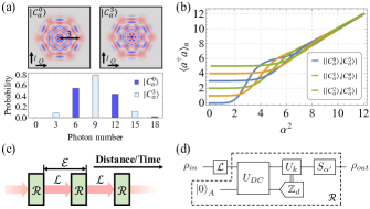
Figure 1: (a) Wigner functions and excitation number distributions of $\left|C_{\alpha}^{0}\right\rangle$ and $\left|C_{\alpha}^{3}\right\rangle$ with $d=\alpha=3$. (b) Average excitation number $\left\langle a^{\dagger}a\right\rangle_{n}$ for cat states with $d=3$. (c) Schematic of alternating LBC ($\mathcal{L}$) and QEC recovery ($\mathcal{R}$). (d) Quantum circuits of QEC recovery for cat codes, consisting of the dispersive coupling gate $U_{DC}$ followed by $\mathbb{Z}_{d}$ measurement of excitation number, rotation gate $U_{k}$ conditioned on $\mathbb{Z}_{d}$ measurement outcome to compensates the lost excitations, and finally amplitude restoration $S_{\alpha^{\prime}}$.

The $2d$-dimensional cat Hilbert space can be divided into $d$ subspaces labeled by $s=0,1,\cdots,d-1$. The “$s$-subspace” has excitation number $s\bmod\ d$, spanned by two logical states $\left|0\right\rangle_{L}^{s}=\left|C_{\alpha}^{s}\right\rangle$ and $\left|1\right\rangle_{L}^{s}=\left|C_{\alpha}^{s+d}\right\rangle$. Fig. 1(a) shows the Wigner functions and excitation distributions of $\left|C_{\alpha}^{s}\right\rangle$ and $\left|C_{\alpha}^{s+d}\right\rangle$ for $d=3$, $\alpha=3$ and $s=0$. It becomes clear that $d$, $\alpha$, and $s$ are three degrees of freedom that determine the performance of cat codes in correcting loss errors.

After losing $k$ excitations, the $s$-subspace is mapped to the $\left(s-k\right)$-subspace: $\left|C_{\alpha}^{s}\right\rangle\rightarrow\left|C_{\alpha}^{s-k}\right\rangle$ and $\left|C_{\alpha}^{s+d}\right\rangle\rightarrow\left|C_{\alpha}^{s+d-k}\right\rangle$ . Hence, we can unambiguously distinguish $0\leq k\leq d-1$ excitation losses without destroying the encoded logical states by projectively measuring the excitation number $\mathrm{mod}$ $d$ (called “$\mathbb{Z}_{d}$ measurement”). In fact, since a cat state maps back to itself after losing integer multiples of $2d$ excitations, we can restore the logical basis states correctly with $2md\leq k\leq\left(2m+1\right)d-1$ excitation losses for integer $m$. If there are $\left(2m+1\right)d\leq k\leq 2\left(m+1\right)d-1$ excitation losses, however, we will misidentify the logical basis states. Since the symmetric superposition $\left|C_{\alpha}^{s}\right\rangle+\left|C_{\alpha}^{s+d}\right\rangle\rightarrow\left|C_{\alpha}^{s-k}\right\rangle+\left|C_{\alpha}^{s+d-k}\right\rangle$ is actually preserved even if we misidentify the logical basis, the misidentification effectively induces an X rotation in the logical basis – a logical bit-flip error.

In addition to the logical bit-flip error, the LBC can induce another type of error via back-action from the environment. For finite $\alpha$, the logical states $\left|C_{\alpha}^{s}\right\rangle$ and $\left|C_{\alpha}^{s+d}\right\rangle$ generally differ in average photon number, as illustrated in Fig. 1(b), as well as the $m$-th moments $\left\langle C_{\alpha}^{s}\right|\left(a^{\dagger}a\right)^{m}\left|C_{\alpha}^{s}\right\rangle\neq\left\langle C_{\alpha}^{d+s}\right|\left(a^{\dagger}a\right)^{m}\left|C_{\alpha}^{d+s}\right\rangle$ for $m\in\mathbb{Z}^{+}$. Hence, the excitation loss to the environment can leak out information about the logical state, which is captured by Kraus operator acting on logical states, $\hat{\mathcal{W}}_{k}\left|C_{\alpha}^{n}\right\rangle\propto\left(1-\gamma\right)^{a^{\dagger}a/2}a^{k}\left|C_{\alpha}^{n}\right\rangle=e^{-\Delta}\alpha^{k}\sqrt{\mathcal{N}_{n-k}\left(\alpha^{\prime}\right)/\mathcal{N}_{n}\left(\alpha\right)}\left|C_{\alpha^{\prime}}^{n-k}\right\rangle$ with $\alpha^{\prime}=\sqrt{1-\gamma}\alpha$ and $\Delta=\alpha^{2}-\alpha^{\prime 2}=\gamma\alpha^{2}$. Defining $G\left(n,m\right)=\sqrt{\mathcal{N}_{m}\left(\alpha^{\prime}\right)/\mathcal{N}_{n}\left(\alpha\right)}$, the fact that $G\left(n,n-k\right)$ is slightly different for $n=s$ and $n=s+d$ results in the back-action associated with losing $k$ excitations . When we average over all possible $k$ values, the back-action induced bias towards $\left|C_{\alpha}^{s}\right\rangle$ or $\left|C_{\alpha}^{s+d}\right\rangle$ are mostly cancelled. However, the back-action does reduce the coherence between $\left|C_{\alpha}^{s}\right\rangle$ and $\left|C_{\alpha}^{s+d}\right\rangle$ and effectively induces a logical dephasing error.

QEC recovery for cat codes.

To protect the quantum information from bosonic loss, we introduce a QEC recovery operation $\mathcal{R}$ (shown in Fig. 1(d)), which consists of a $\mathbb{Z}_{d}$ measurement, conditional loss compensation, and amplitude restoration. First, we use the $\mathbb{Z}_{d}$ measurement to distinguish different loss events up to losing $d-1$ excitations. Similar to the qubit-assisted number parity ($\mathbb{Z}_{2}$) measurement Sun et al. (2014), we consider a $d$-level ancilla (e.g., using higher levels of the transmon Wang et al. (2016)) that dispersively couples to a cavity mode

$$\hat{H}_{DC}=\stackrel{{\scriptstyle[}}{{j}}=0]{d-1}{\sum}j\chi\left|j\right\rangle\left\langle j\right|a^{\dagger}a,$$ (3)

where $\left|j\right\rangle$ are the basis states of the ancilla. Combined with Fourier gates on the $d$-level ancilla, $F_{d}$, we can implement the unitary operation $U_{DC}=F_{d}^{\dagger}e^{-i\frac{\pi}{\chi}H_{DC}}F_{d}$ that maps the $\mathbb{Z}_{d}$ information to the ancilla that is subsequently measured in $\left\{\left|j\right\rangle\right\}$ basis.

Then, conditioned on measured excitation loss number (mod $d$), $k\in\left\{0,1,\cdots,d-1\right\}$, we implement the following unitary to compensate the identified loss and restore the state back to the $s$-subspace

$$U_{k}=\left|C_{\alpha^{\prime}}^{s}\right\rangle\left\langle C_{\alpha^{\prime}}^{s-k}\right|+\left|C_{\alpha^{\prime}}^{d+s}\right\rangle\left\langle C_{\alpha^{\prime}}^{d+s-k}\right|+U_{k}^{0},$$ (4)

where $U_{k}^{0}$ is an arbitrary unitary on the complementary subspace of $\left\{\left|C_{\alpha^{\prime}}^{s-k}\right\rangle,\left|C_{\alpha^{\prime}}^{d+s-k}\right\rangle\right\}$ so that $U_{k}$ is a unitary in the entire Hilbert space. $U_{k}$ can be achieved with unitary control of the bosonic mode (e.g., as demonstrated in superconducting circuits Krastanov et al. (2015); Heeres et al. (2015, 2016)).

Finally, we restore the amplitude from $\alpha^{\prime}$ back to $\alpha$ via the following unitary

$$S_{\alpha^{\prime}}=\sum_{s=0}^{d-1}\left(\left|C_{\alpha}^{s}\right\rangle\left\langle C_{\alpha^{\prime}}^{s}\right|+\left|C_{\alpha}^{d+s}\right\rangle\left\langle C_{\alpha^{\prime}}^{d+s}\right|\right)+S_{\alpha^{\prime}}^{0},$$ (5)

where $S_{\alpha^{\prime}}^{0}$ is an arbitrary unitary on the complementary subspace of the $2d$-dimensional subspace spanned by $\left|C_{\alpha^{\prime}}^{n}\right\rangle$. Alternative to the unitary implementation of $S_{\alpha^{\prime}}$, we may also use engineered dissipation to restore the amplitude from $\alpha^{\prime}$ to $\alpha$ without compromising the encoded logical state Leghtas et al. (2015); Mirrahimi et al. (2014).

Overall, the QEC recovery in Fig. 1(d) implements

$$\mathcal{R}\left(\rho\right)=\stackrel{{\scriptstyle[}}{{k}}=0]{d-1}{\sum}\left|C_{\alpha}^{s}\right\rangle\left\langle C_{\alpha^{\prime}}^{s-k}\right|\rho\left|C_{\alpha^{\prime}}^{s-k}\right\rangle\left\langle C_{\alpha}^{s}\right|,$$ (6)

which restores the original encoded subspace. Note that the $d$-level ancilla can also be replaced by a $2$-level ancilla, with an overhead of $\log_{2}d$ steps of measurement and feedforward control to fully implement the QEC recovery $\mathcal{R}$ with Kraus rank $d$ Lloyd and Viola (2001); Shen and et. al. .

Logical bit-flip and dephasing errors.

We now analyze the effective errors in the encoded subspace after the QEC recovery. Writing density matrix as a column vector $\rho=\left(\begin{array}[]{cccc}\rho_{00}&\rho_{01}&\rho_{10}&\rho_{11}\end{array}\right)^{\mathrm{T}}$, $\rho_{out}$ is linked to $\rho_{in}$ via $\mathcal{E}=\mathcal{R}\circ\mathcal{L}=\left(\mathcal{E}_{ij}\right)\left(i,j=1,2,3,4\right)$

$$\mathcal{E} = \stackrel{{\scriptstyle[}}{{k}}=0]{d-1}{\sum}T_{k}\left(\begin{array}[]{cccc}A_{sk}^{2}&0&0&0\\ 0&A_{sk}D_{sk}&0&0\\ 0&0&A_{sk}D_{sk}&0\\ 0&0&0&D_{sk}^{2}\end{array}\right)$$ (16)

$$+\stackrel{{\scriptstyle[}}{{k}}=0]{d-1}{\sum}T_{k+d}\left(\begin{array}[]{cccc}0&0&0&C_{sk}^{2}\\ 0&0&B_{sk}C_{sk}&0\\ 0&B_{sk}C_{sk}&0&0\\ B_{sk}^{2}&0&0&0\end{array}\right),$$

where $A_{sk}=G\left(s,s-k\right)$, $B_{sk}=G\left(s,d+s-k\right)$, $C_{sk}=G\left(d+s,s-k\right)$ and $D_{sk}=G\left(d+s,d+s-k\right)$ are back-action coefficients. $T_{k}=\stackrel{{\scriptstyle[}}{{m}}=0]{\infty}{\sum}\frac{e^{-\Delta}\Delta^{2md+k}}{\left(2md+k\right)!}$ and $T_{k+d}=\stackrel{{\scriptstyle[}}{{m}}=0]{\infty}{\sum}\frac{e^{-\Delta}\Delta^{\left(2m+1\right)d+k}}{\left[\left(2m+1\right)d+k\right]!}$ is the probability for correct and incorrect recovery, respectively, for an ideal Poisson distribution with mean $\Delta$ for excitation losses. It is clear from Eq. (16) that the probabilities for excitation losses for cat codes are modulated by the back-action.

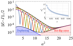
Figure 2: Diamond distance $\left\|\mathcal{E}-\mathcal{I}\right\|_{\diamond}/2$ calculated numerically from the $\mathcal{E}$ in Eq. (16) for logical subspace $s=0,1,2,3$ (blue, red, green and yellow curves, respectively) and analytical bounds $\Gamma_{\pm}$ (black), for $d=4$ and $\gamma=0.005$. The two types of errors in $\Gamma_{-}$, i.e. logical bit-flip error $\epsilon_{f}$ and logical dephasing $\epsilon_{d}$, are marked. The dashed purple and black curves show $\bar{\Gamma}$ and the minimum $\Gamma_{-}$, respectively. The inset shows $\alpha_{o}^{2}\left(\gamma\right)$ for $d=4$; analytical results (solid) from Eq. (22) agree with numerical calculations (circles).

Considering small logical bit-flip error and overlap between neighboring coherent states, to the leading order of error we can write $\mathcal{E}$ as a Pauli channel Sup

$$\mathcal{E}\left(\rho\right)\approx\left[1-\left(\epsilon_{f}+\epsilon_{d}\right)\right]\rho+\epsilon_{f}X\rho X+\epsilon_{d}Z\rho Z,$$ (17)

with logical bit-flip error due to excessive loss of (more than $d-1$) excitations

$$\epsilon_{f} = \stackrel{{\scriptstyle[}}{{k}}=0]{d-1}{\sum}T_{k+d},$$ (18)

and logical dephasing error induced by back-action

$$\epsilon_{d} = \frac{1}{2}e^{-4\alpha^{2}\sin^{2}\frac{\pi}{2d}}\left(e^{4\Delta\sin^{2}\frac{\pi}{2d}}-1\right)$$ (19)

$$-\frac{1}{2}e^{-4\alpha^{2}\sin^{2}\frac{\pi}{2d}}\sqrt{1-2e^{\mu}\cos\psi+e^{2\mu}}\cos\theta,$$

where $\mu=2\Delta\left(2\sin^{2}\frac{\pi}{2d}-\sin^{2}\frac{\pi}{d}\right)$, $\psi=\Delta(2\sin\frac{\pi}{d}-\sin\frac{2\pi}{d})$, $\theta=\frac{2s\pi}{d}-2\alpha^{2}\sin\frac{\pi}{d}+\arctan\frac{e^{\mu}\sin\psi}{1-e^{\mu}\cos\psi}$. With Eq. (16), we can quantify the residual decoherence after the QEC recovery using the diamond distance Sacchi (2005); Benenti and Strini (2010)

$$\Gamma\left(\alpha,\ d,\ \gamma,\ s\right)\equiv\left\|\mathcal{E}-\mathcal{I}\right\|_{\diamond}/2\approx\epsilon_{f}+\epsilon_{d}.$$ (20)

For given $\gamma$ and $d$, we may select coherent amplitude $\alpha$ and logical subspace $s$ to minimize $\left\|\mathcal{E}-\mathcal{I}\right\|_{\diamond}/2$. As illustrated in Fig. 2, for each fixed $s$-subspace encoding, the diamond distance oscillates with $\alpha^{2}$ and there is a set of $\alpha$ where the back-action induced dephasing reaches a local minimum, suppressed to $\mathcal{O}\left[\left(\Delta\pi^{2}/d^{2}\right)^{2}\right]$ Sup . In fact, each favorable combination of $s$ and $\alpha$ gives the same average excitation number for the logical states, $\left\langle C_{\alpha}^{s}\right|a^{\dagger}a\left|C_{\alpha}^{s}\right\rangle=\left\langle C_{\alpha}^{d+s}\right|a^{\dagger}a\left|C_{\alpha}^{d+s}\right\rangle$ (associated with the crossing points in Fig. 1(b)), while the residual back-action only comes from the difference in second and higher moments of $a^{\dagger}a$.

To estimate the minimum achievable error, we obtain analytical expressions for two approximate envelop functions

$$\Gamma_{\pm}\left(\alpha,\ \gamma,\ d\right) = \epsilon_{f}+\left.\epsilon_{d}\right|_{\cos\theta=\mp 1},$$ (21)

which provide upper and lower bounds on the diamond distance $\Gamma\left(\alpha,\ d,\ \gamma,\ s\right)$ for all $s$. As illustrated in Fig. 2, to achieve the minimum error $\Gamma_{-}$ (lower black curve), it is crucial to perform combined optimization of $\alpha$ and $s$. If we are non-selective in the logical subspace (i.e., averaging over all $s$) and only optimize the coherent amplitude $\alpha$, the averaged error is approximately $\Gamma_{+}/2$ (dashed purple curve), which can be an order of magnitude larger than $\Gamma_{-}$ for the parameter region of interest. Moreover, the combined optimization also leads to a smaller optimized coherent amplitude.

Using Eq. (21), we can estimate the optimal amplitude $\alpha_{o}$ by requiring the two competing errors be equal in $\Gamma_{-}$. For $\Delta\ll d$, we obtain the following approximate expression for $\alpha_{o}^{2}\left(d,\gamma\right)$ for $d>2$

$$\alpha_{o}^{2} \approx \frac{W\left[\frac{4\sin^{2}\left(\frac{\pi}{2d}\right)-\gamma}{\left(d-2\right)\gamma}\left(\frac{d!}{2}\frac{\pi^{4}}{d^{4}}\right)^{\frac{1}{d-2}}\right]}{\frac{4\sin^{2}\left(\frac{\pi}{2d}\right)-\gamma}{d-2}},$$ (22)

where $W$ is the Lambert W function $z=f^{-1}\left(ze^{z}\right)=W\left(ze^{z}\right)$. The inset of Fig. 2 shows that even at $d=4$, there is already good agreement between Eq. (22) and numerical results. Based on the estimated $\alpha_{o}$, we can identify the best combination of $\alpha^{*}$ and $s^{*}$ near the vicinity of the minimum $\Gamma_{-}$.

Application to repetitive correction.

So far we have considered the performance of cat codes for a single round of LBC followed by QEC recovery, and have identified the optimal amplitude $\alpha_{o}$ and logical subspace $s$ for given $d$ and $\gamma$. For practical applications, however, we may use multiple rounds of LBC and QEC recovery, and optimize the frequency of recovery to best maintain the coherence. In the following, we consider one-way QRs with cat codes Munro et al. (2012); Muralidharan et al. (2014) over transcontinental distances ($\geq 10^{3}\mathrm{km}$). We note that the effect of localized gates that induce photon loss can be treated similarly as coupling inefficiency and thus the results obtained below for one-way QRs are naturally applicable to localized repetitive QEC with leaky gates.

We introduce intermediate repeater stations with a small spacing $L_{0}$ ($\ll L_{\mathrm{att}}$), so that the fiber attenuation induced loss errors are correctable. Given near-unity coupling efficiency $\eta$ we have $\gamma\approx\tilde{L}_{0}+2\left(1-\eta\right)$, with $\tilde{L}_{0}=L_{0}/L_{\mathrm{att}}$ for the dimensionless repeater spacing. The goal is to minimize the effective error rate

$$\tau_{-}\left(\alpha,\ \tilde{L}_{0},\ d\right)=\Gamma_{-}\left(\alpha,\ \gamma,\ d\right)/\tilde{L}_{0}.$$ (23)

Fig. 3(a) shows the minimized effective error rate as a function of $d$ for $\eta=99.5\%$ with the corresponding optimized arc length between neighboring coherent states $\pi\alpha_{\mathrm{opt}}/d$. Note that the minimized error rate is anti-correlated with the arc length $\pi\alpha_{\mathrm{opt}}/d$, because increasing arc length suppresses the coherent component overlap and consequently reduces the back-action induced dephasing. For small $d$, the overall bit-flip error can be better suppressed by increasing $d$ to correct more excitation loss errors; for large $d$, however, the typical number of excitation losses is $\gamma\alpha^{2}\propto\gamma d^{2}$, which will exceed the capability of QEC. Hence, there is an optimized choice of $d$ that minimizes the overall error.

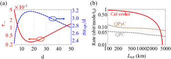
Figure 3: Optimized performance of cat codes for QRs with $\eta=99.5\%$ and comparison with selected DV schemes. (a). Minimum effective error rate $\tau_{-}$ (red) and associated optimum arc length $\frac{\pi\alpha_{\mathrm{opt}}}{d}$ (blue). (b). Optimized SKRPM over long distances for one-way QRs with cat codes (red solid), quantum polynomial codes Muralidharan et al. (2015) (brown dotted) and quantum parity code Muralidharan et al. (2014, 2016) (gray dashed). $t_{0}$ is the gate operation time taken as the same for three schemes.

For one-way QRs with cat codes, the entire repeater chain can be characterized by

$$\mathcal{E}^{N}=\left(\mathcal{R}\circ\mathcal{L}\right)^{N},$$ (24)

with $N=L_{\mathrm{tot}}/\left(\tilde{L}_{0}^{\mathrm{opt}}L_{\mathrm{att}}\right)$ intermediate repeater stations. More specifically, we consider a four-state quantum key distribution protocol. With $\mathcal{E}^{N}$ written as a $4\times 4$ matrix with entries $\mathcal{E}_{ij}^{N}$, quantum bit error rates in the Z- and X-basis can be derived as $Q_{Z}=\left(\mathcal{E}_{14}^{N}+\mathcal{E}_{41}^{N}\right)/2$ and $Q_{X}=\left[\left(\mathcal{E}_{11}^{N}+\mathcal{E}_{14}^{N}+\mathcal{E}_{41}^{N}+\mathcal{E}_{44}^{N}\right)-\left(\mathcal{E}_{22}^{N}+\mathcal{E}_{23}^{N}+\mathcal{E}_{32}^{N}+\mathcal{E}_{33}^{N}\right)\right]/4$ , respectively. Since using multiple modes may carry a large resource overhead, here we use the secure key rate per mode (SKRPM) to evaluate the performance of one-way QRs Namiki et al. (2016). For single-mode encoding schemes, the SKRPM is $\mathrm{Rate}=1-H\left(Q_{Z}\right)-H\left(Q_{X}\right)$, where $H\left(p\right)=-p\log_{2}p-\left(1-p\right)\log_{2}\left(1-p\right)$ is the binary entropy function Wang (2005). Fig. 3(b) shows the optimized SKRPM for one-way QRs with cat codes with $\eta=99.5\%$ for distributing quantum keys over long distances and, in comparison, the optimized SKRPM for multi-mode DV encoding quantum parity code (QPC) Muralidharan et al. (2014, 2016) and quantum polynomial code (QPyC) Muralidharan et al. (2015). With high coupling efficiency, as a single-mode encoding, cat codes outperform conventional DV quantum codes due to efficient use of the bosonic mode.

Conclusion and outlook.

We have investigated cat codes for protecting quantum states against bosonic excitation loss. At the encoded level, there are two major types of uncorrectable errors, logical bit-flip error, due to excessive excitation loss and logical dephasing error, induced by back-action. We have demonstrated that non-trivial combinations of coherent amplitude and logical subspace can efficiently suppress logical dephasing error, and lead to significantly improved QEC performance. We expect this feature of suppressed back-action from the environment to be observed for other approximate CV quantum codes as $\left\langle 0_{L}\right|a^{\dagger}a\left|0_{L}\right\rangle=\left\langle 1_{L}\right|a^{\dagger}a\left|1_{L}\right\rangle$ is satisfied and the balance between the back-action and excessive excitation loss could be useful for the optimization of their QEC capabilities. Comparison between cat codes and other known single-mode schemes, such as GKP codes Gottesman et al. (2001); Terhal and Duivenvoorden (2016); Terhal and Weigand (2016) and binomial codes Michael et al. (2016), over LBC could shed further light on the optimal construction of single-mode CV encodings. We notice that cat codes become less favorable, compared with conventional multi-mode schemes, in case of long communication distance (Fig. 3(b)) or high coupling loss Sup , as a result of high occupation of a single bosonic mode. This can motivate us to explore unconventional multi-mode CV encodings with multiple excitations per mode Harrington and Preskill (2001) that may asymptotically achieve the channel capacity of LBC.

As an application, we have explored one-way quantum communication over long distances with cat codes and found that given high-fidelity coupling into and out of the repeaters this single-mode continuous variable scheme can outperform conventional schemes with single excitation occupying multiple modes in terms of secure key rate per mode. With recent developments of efficient coupling between fiber and optical waveguide Tiecke et al. (2015), and high-fidelity frequency conversion between optical and microwave modes Andrews et al. (2014); O’Brien et al. (2014); Zou et al. (2016), we may envision realistic quantum repeaters consisting of superconducting circuits for error correction and optical-microwave quantum transducers to protect transmitted quantum information against optical loss in fiber channels.

We thank Kasper Duivenvoorden, Jungsang Kim, Norbert Lütkenhaus, Marios H. Michael, Ananda Roy, Chao Shen, Barbara Terhal, Hong Tang for stimulating discussions. We acknowledge support from the ARL-CDQI, ARO (W911NF-14-1-0011, W911NF-14-1-0563), ARO MURI (W911NF-16-1-0349), NSF (DMR-1609326, DGE-1122492), AFOSR MURI (FA9550-14-1- 0052, FA9550-14-1-0015), Alfred P. Sloan Foundation (BR2013-049), and Packard Foundation (2013-39273).

Note added: During the preparation of the manuscript, the authors became aware of a related work on cat codes Bergmann and van Loock (2016). Different from that work, here we have proposed a deterministic amplitude restoration for QEC recovery and investigated combined optimization of amplitude and logical subspace.

Supplementary Material

I Analysis of quantum channel $\mathcal{E}$ and diamond norm $\left\|\mathcal{E}-\mathcal{I}\right\|_{\diamond}$

In the following, we analytically show that $\mathcal{E}$ can be approximated as a Pauli channel and calculate the diamond norm $\left\|\mathcal{E}-\mathcal{I}\right\|_{\diamond}$. We begin by specifying two assumptions that are used throughout the analysis

1. $\epsilon_{f}=\stackrel{{\scriptstyle[}}{{k}}=0]{d-1}{\sum}T_{k+d}=\mathcal{O}\left(\frac{e^{-\Delta}\Delta^{d}}{d!}\right)\ll 1$, which physically implies that bit-flip error is considerably small.

2. Defining $\delta=\left|\Braket{\alpha}{\alpha e^{i\frac{\pi}{d}}}\right|=\left|\exp\left(\alpha^{2}e^{i\frac{\pi}{d}}-\alpha^{2}\right)\right|$, then $\delta\approx e^{-\frac{1}{2}\left(\frac{\pi\alpha}{d}\right)^{2}}\ll 1$, which physically implies that the overlap between neighboring coherent states is considerably small.

Then, the normalization factor

$$\mathcal{N}_{n}\left(\alpha\right) = \stackrel{{\scriptstyle[}}{{k}}=0]{2d-1}{\sum}\omega^{-kn}\exp\left[\left(\omega^{k}-1\right)\alpha^{2}\right]$$ (S.1)

$$= \stackrel{{\scriptstyle[}}{{j}}=0]{2d-1}{\sum}e^{-2\alpha^{2}\sin^{2}\frac{j\pi}{2d}}\cos\left(\frac{jn\pi}{d}-\alpha^{2}\sin\frac{j\pi}{d}\right)$$

$$= 1+\zeta_{n}\left(\alpha\right)+\mathcal{O}\left(\delta^{4}\right),$$

where $\zeta_{n}\left(\alpha\right)=2e^{-2\alpha^{2}\sin^{2}\frac{\pi}{2d}}\cos\left(\frac{n\pi}{d}-\alpha^{2}\sin\frac{\pi}{d}\right)=\mathcal{O}\left(\delta\right)$. With Approx. 1-2 and Eq. (S.1), we note

$$\stackrel{{\scriptstyle[}}{{k}}=0]{d-1}{\sum}T_{k+d}C_{sk}^{2} = \stackrel{{\scriptstyle[}}{{k}}=0]{d-1}{\sum}T_{k+d}\frac{\mathcal{N}_{s-k}\left(\alpha^{\prime}\right)}{\mathcal{N}_{d+s}\left(\alpha\right)}$$

$$= \frac{\stackrel{{\scriptstyle[}}{{k}}=0]{d-1}{\sum}T_{k+d}+\stackrel{{\scriptstyle[}}{{k}}=0]{d-1}{\sum}T_{k+d}\left[\mathcal{N}_{s-k}\left(\alpha^{\prime}\right)-1\right]}{1+\left[\mathcal{N}_{d+s}\left(\alpha\right)-1\right]}$$

$$= \frac{\stackrel{{\scriptstyle[}}{{k}}=0]{d-1}{\sum}T_{k+d}+\stackrel{{\scriptstyle[}}{{k}}=0]{d-1}{\sum}T_{k+d}\mathcal{O}\left(\delta\right)}{1+\mathcal{O}\left(\delta\right)}$$

$$= \epsilon_{f}+\mathcal{O}\left(\epsilon_{f}\delta\right).$$

Similarly, $\stackrel{{\scriptstyle[}}{{k}}=0]{d-1}{\sum}T_{k+d}B_{sk}C_{sk}=\epsilon_{f}+\mathcal{O}\left(\epsilon_{f}\delta\right)$ and $\stackrel{{\scriptstyle[}}{{k}}=0]{d-1}{\sum}T_{k+d}B_{sk}^{2}=\epsilon_{f}+\mathcal{O}\left(\epsilon_{f}\delta\right)$. Therefore, we may simplify $\mathcal{E}$ as

$$\mathcal{E} = \left(\begin{array}[]{cccc}\lambda_{1}&0&0&\epsilon_{f}\\ 0&\lambda_{2}&\epsilon_{f}&0\\ 0&\epsilon_{f}&\lambda_{2}&0\\ \epsilon_{f}&0&0&\lambda_{3}\end{array}\right)+\mathcal{O}\left(\epsilon_{f}\delta\right),$$ (S.6)

where $\lambda_{1}=\stackrel{{\scriptstyle[}}{{k}}=0]{d-1}{\sum}T_{k}A_{sk}^{2}$, $\lambda_{2}=\stackrel{{\scriptstyle[}}{{k}}=0]{d-1}{\sum}T_{k}A_{sk}D_{sk}$ and $\lambda_{3}=\stackrel{{\scriptstyle[}}{{k}}=0]{d-1}{\sum}T_{k}D_{sk}^{2}$, and the back-action coefficients are $A_{sk}=\sqrt{\mathcal{N}_{s-k}\left(\alpha^{\prime}\right)/\mathcal{N}_{s}\left(\alpha\right)}$, $B_{sk}=\sqrt{\mathcal{N}_{d+s-k}\left(\alpha^{\prime}\right)/\mathcal{N}_{s}\left(\alpha\right)}$, $C_{sk}=\sqrt{\mathcal{N}_{s-k}\left(\alpha^{\prime}\right)/\mathcal{N}_{d+s}\left(\alpha\right)}$ and $D_{sk}=\sqrt{\mathcal{N}_{d+s-k}\left(\alpha^{\prime}\right)/\mathcal{N}_{d+s}\left(\alpha\right)}$.

I.1 $\lambda_{1}$ and $\lambda_{3}$

First of all, we rewrite the expression of $\lambda_{1}$ as

$$1-\lambda_{1} = 1-\frac{\stackrel{{\scriptstyle[}}{{k}}=0]{d-1}{\sum}T_{k}\mathcal{N}_{s-k}\left(\alpha^{\prime}\right)}{\mathcal{N}_{s}\left(\alpha\right)}$$ (S.7)

$$= 1-\frac{\stackrel{{\scriptstyle[}}{{k}}=0]{d-1}{\sum}T_{k}+\stackrel{{\scriptstyle[}}{{k}}=0]{d-1}{\sum}T_{k}\left[\mathcal{N}_{s-k}\left(\alpha^{\prime}\right)-1\right]}{1+\left[\mathcal{N}_{s}\left(\alpha\right)-1\right]}.$$

Since $T_{k}=\stackrel{{\scriptstyle[}}{{m}}=0]{\infty}{\sum}\frac{e^{-\Delta}\Delta^{2md+k}}{\left(2md+k\right)!}$ and $\epsilon_{f}=1-\stackrel{{\scriptstyle[}}{{k}}=0]{d-1}{\sum}T_{k}$, we have

$$\stackrel{{\scriptstyle[}}{{k}}=0]{d-1}{\sum}T_{k}\left[\mathcal{N}_{s-k}\left(\alpha^{\prime}\right)-1\right] = \stackrel{{\scriptstyle[}}{{k}}=0]{d-1}{\sum}\stackrel{{\scriptstyle[}}{{m}}=0]{\infty}{\sum}\frac{e^{-\Delta}\Delta^{2md+k}}{\left(2md+k\right)!}\left[\mathcal{N}_{s-k}\left(\alpha^{\prime}\right)-1\right]$$ (S.8)

$$= \stackrel{{\scriptstyle[}}{{k}}=0]{\infty}{\sum}\frac{e^{-\Delta}\Delta^{k}}{k!}\stackrel{{\scriptstyle[}}{{j}}=1]{2d-1}{\sum}e^{-2\alpha^{\prime 2}\sin^{2}\frac{j\pi}{2d}}\cos\left[\frac{j\left(s-k\right)\pi}{d}-\alpha^{\prime 2}\sin\frac{j\pi}{d}\right]+\mathcal{O}\left(\epsilon_{f}\delta\right)$$

$$= \stackrel{{\scriptstyle[}}{{j}}=1]{2d-1}{\sum}e^{\alpha^{\prime 2}\cos\frac{j\pi}{d}-\alpha^{2}}\stackrel{{\scriptstyle[}}{{k}}=0]{\infty}{\sum}\frac{\Delta^{k}}{k!}\cos\left[\frac{j\left(s-k\right)\pi}{d}-\alpha^{\prime 2}\sin\frac{j\pi}{d}\right]+\mathcal{O}\left(\epsilon_{f}\delta\right)$$

$$= \stackrel{{\scriptstyle[}}{{j}}=1]{2d-1}{\sum}e^{\alpha^{\prime 2}\cos\frac{j\pi}{d}-\alpha^{2}}e^{\Delta\cos\frac{j\pi}{d}}\cos\left(\frac{js\pi}{d}-\alpha^{2}\sin\frac{j\pi}{d}\right)+\mathcal{O}\left(\epsilon_{f}\delta\right)$$

$$= \mathcal{N}_{s}\left(\alpha\right)-1+\mathcal{O}\left(\epsilon_{f}\delta\right),$$

where we use the equality

$$\stackrel{{\scriptstyle[}}{{k}}=0]{\infty}{\sum}\frac{\Delta^{k}}{k!}\cos\left[\frac{j\left(s-k\right)\pi}{d}-\alpha^{\prime 2}\sin\frac{j\pi}{d}\right] = e^{\Delta\cos\frac{j\pi}{d}}\cos\left(\frac{js\pi}{d}-\alpha^{2}\sin\frac{j\pi}{d}\right).$$

Therefore, we arrive at

$$1-\lambda_{1} = \frac{1+\left[\mathcal{N}_{s}\left(\alpha\right)-1\right]-\stackrel{{\scriptstyle[}}{{k}}=0]{d-1}{\sum}T_{k}-\stackrel{{\scriptstyle[}}{{k}}=0]{d-1}{\sum}T_{k}\left[\mathcal{N}_{s-k}\left(\alpha^{\prime}\right)-1\right]}{1+\left[\mathcal{N}_{s}\left(\alpha\right)-1\right]}$$ (S.9)

$$= \frac{\epsilon_{f}+\mathcal{O}\left(\epsilon_{f}\delta\right)}{1+\mathcal{O}\left(\delta\right)}$$

$$= \epsilon_{f}+\mathcal{O}\left(\epsilon_{f}\delta\right)$$

Similarly we can also obtain

$$1-\lambda_{3}=\epsilon_{f}+\mathcal{O}\left(\epsilon_{f}\delta\right).$$ (S.10)

I.2 $\lambda_{2}$

The expression of $\lambda_{2}$ is

$$1-\lambda_{2} = 1-\frac{\stackrel{{\scriptstyle[}}{{k}}=0]{d-1}{\sum}T_{k}\sqrt{\mathcal{N}_{s-k}\left(\alpha^{\prime}\right)\mathcal{N}_{d+s-k}\left(\alpha^{\prime}\right)}}{\sqrt{\mathcal{N}_{s}\left(\alpha\right)\mathcal{N}_{d+s}\left(\alpha\right)}}.$$ (S.11)

From Eq. (S.1) we know that

$$\mathcal{N}_{s}\left(\alpha\right) = 1+\zeta_{s}\left(\alpha\right)+\mathcal{O}\left(\delta^{4}\right),$$

$$\mathcal{N}_{d+s}\left(\alpha\right) = 1-\zeta_{s}\left(\alpha\right)+\mathcal{O}\left(\delta^{4}\right),$$

and

$$\sqrt{\mathcal{N}_{s}\left(\alpha\right)\mathcal{N}_{d+s}\left(\alpha\right)} = 1-\frac{\zeta_{s}\left(\alpha\right)^{2}}{2}+\mathcal{O}\left(\delta^{4}\right)$$ (S.12)

we have

$$1-\lambda_{2} = 1-\frac{\stackrel{{\scriptstyle[}}{{k}}=0]{d-1}{\sum}T_{k}\left[1-\frac{\zeta_{s-k}\left(\alpha^{\prime}\right)^{2}}{2}+\mathcal{O}\left(\delta^{4}\right)\right]}{1-\frac{\zeta_{s}\left(\alpha\right)^{2}}{2}+\mathcal{O}\left(\delta^{4}\right)}$$ (S.13)

$$= \frac{\epsilon_{f}-\frac{\zeta_{s}\left(\alpha\right)^{2}}{2}+\mathcal{O}\left(\delta^{4}\right)+\stackrel{{\scriptstyle[}}{{k}}=0]{d-1}{\sum}T_{k}\left[\frac{\zeta_{s-k}\left(\alpha^{\prime}\right)^{2}}{2}+\mathcal{O}\left(\delta^{4}\right)\right]}{1-\frac{\zeta_{s}\left(\alpha\right)^{2}}{2}+\mathcal{O}\left(\delta^{4}\right)}.$$

Similar to the approximation in Eq. (S.8), we have

$$\stackrel{{\scriptstyle[}}{{k}}=0]{d-1}{\sum}T_{k}\frac{\zeta_{s-k}\left(\alpha^{\prime}\right)^{2}}{2} = 2e^{-4\alpha^{\prime 2}\sin^{2}\frac{\pi}{2d}}\stackrel{{\scriptstyle[}}{{k}}=0]{\infty}{\sum}\frac{e^{-\Delta}\Delta^{k}}{k!}\cos^{2}\left[\frac{\left(s-k\right)\pi}{d}-\alpha^{\prime 2}\sin\frac{\pi}{d}\right]+\mathcal{O}\left(\epsilon_{f}\delta^{2}\right)$$ (S.14)

$$= e^{-4\alpha^{\prime 2}\sin^{2}\frac{\pi}{2d}}\left\{1+e^{-2\Delta\sin^{2}\frac{\pi}{d}}\cos\left[\frac{2s\pi}{d}-2\alpha^{\prime 2}\sin\frac{\pi}{d}-\Delta\sin\frac{2\pi}{d}\right]\right\}+\mathcal{O}\left(\epsilon_{f}\delta^{2}\right),$$

and hence

$$-\frac{\zeta_{s}\left(\alpha\right)^{2}}{2}+\stackrel{{\scriptstyle[}}{{k}}=0]{d-1}{\sum}T_{k}\frac{\zeta_{s+k}\left(\alpha^{\prime}\right)^{2}}{2} = e^{-4\alpha^{2}\sin^{2}\frac{\pi}{2d}}\left\{e^{4\Delta\sin^{2}\frac{\pi}{2d}}-1-\left[\cos\Phi-e^{\mu}\cos\left(\Phi+\psi\right)\right]\right\}+\mathcal{O}\left(\epsilon_{f}\delta^{2}\right)$$

$$= e^{-4\alpha^{2}\sin^{2}\frac{\pi}{2d}}\left[e^{4\Delta\sin^{2}\frac{\pi}{2d}}-1-\left(1-2e^{\mu}\cos\psi+e^{2\mu}\right)^{\frac{1}{2}}\cos\left(\Phi+\varphi\right)\right]+\mathcal{O}\left(\epsilon_{f}\delta^{2}\right)$$

where we denote $\mu=2\Delta\left(2\sin^{2}\frac{\pi}{2d}-\sin^{2}\frac{\pi}{d}\right)$, $\psi=\Delta(2\sin\frac{\pi}{d}-\sin\frac{2\pi}{d})$, $\Phi=\frac{2s\pi}{d}-2\alpha^{2}\sin\frac{\pi}{d}$ and $\varphi=\arctan\frac{e^{\mu}\sin\psi}{1-e^{\mu}\cos\psi}$. Therefore

$$1-\lambda_{2} = \epsilon_{f}+e^{-4\alpha^{2}\sin^{2}\frac{\pi}{2d}}\left[e^{4\Delta\sin^{2}\frac{\pi}{2d}}-1-\left(1-2e^{\mu}\cos\psi+e^{2\mu}\right)^{\frac{1}{2}}\cos\left(\Phi+\varphi\right)\right]+\mathcal{O}\left(\epsilon_{f}\delta^{2}\right).$$

$$\equiv \epsilon_{f}+2\epsilon_{d}+\mathcal{O}\left(\epsilon_{f}\delta^{2}\right).$$

Plugging the analytical expressions of $\lambda_{n}\ (n=1,2,3)$ into Eq. (S.6), we can approximate $\mathcal{E}$ as a qubit Pauli channel as in Eq. (16).

II Quantification of decoherence suppression

We quantify the improvement in suppressing decoherence using our approach by further simplifying $\Gamma_{-}=\epsilon_{f}+\frac{1}{2}e^{-4\alpha^{2}\sin^{2}\frac{\pi}{2d}}\left[e^{4\Delta\sin^{2}\frac{\pi}{2d}}-1-\left(1-2e^{\mu}\cos\psi+e^{2\mu}\right)^{\frac{1}{2}}\right]$. Considering $\frac{\pi}{d}\ll 1$, we shall approximate

$$e^{4\Delta\sin^{2}\frac{\pi}{2d}}-1 = \Delta\left(\frac{\pi}{d}\right)^{2}\left[1+\frac{1}{2}\left(\Delta\left(\frac{\pi}{d}\right)^{2}-\frac{1}{6}\right)\left(\frac{\pi}{d}\right)^{2}\right]+\mathcal{O}\left(\frac{\pi}{d}\right)^{6}$$

$$\left(1-2e^{\mu}\cos\psi+e^{2\mu}\right)^{\frac{1}{2}} = \Delta\left(\frac{\pi}{d}\right)^{2}\left[1-\frac{1}{2}\left(\Delta\left(\frac{\pi}{d}\right)^{2}+\frac{1}{6}\right)\left(\frac{\pi}{d}\right)^{2}\right]+\mathcal{O}\left(\frac{\pi}{d}\right)^{6},$$

and hence

$$\Gamma_{-}=\epsilon_{f}+\frac{1}{2}e^{-4\alpha^{2}\sin^{2}\frac{\pi}{2d}}\left[\Delta^{2}\left(\frac{\pi}{d}\right)^{4}+\mathcal{O}\left(\frac{\pi}{d}\right)^{6}\right].$$ (S.16)

On the other hand,

$$\bar{\Gamma} = \epsilon_{f}+\frac{1}{2}e^{-4\alpha^{2}\sin^{2}\frac{\pi}{2d}}\left(e^{4\Delta\sin^{2}\frac{\pi}{2d}}-1\right)$$ (S.17)

$$= \epsilon_{f}+\frac{1}{2}e^{-4\alpha^{2}\sin^{2}\frac{\pi}{2d}}\left[\Delta\left(\frac{\pi}{d}\right)^{2}+\mathcal{O}\left(\frac{\pi}{d}\right)^{4}\right].$$

At the regime where back-action induced dephasing dominates, we can see from Eq. (S.16-S.17) that the decoherence is reduced from $\mathcal{O}\left(\Delta\pi^{2}/d^{2}\right)$ to $\mathcal{O}\left[\left(\Delta\pi^{2}/d^{2}\right)^{2}\right]$.

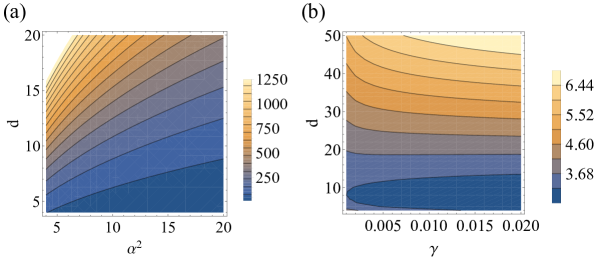
Figure S1: Improvement in suppressing decoherence using cat codes with the proposed recovery. (a). $\Delta\pi^{2}/d^{2}$ with $\gamma=0.005$. (b). $\bar{\Gamma}\left(\alpha_{subo},\gamma,d\right)/\Gamma_{-}\left(\alpha_{o},\gamma,d\right)$

In Fig. S1(a) we show $\frac{1}{\Delta\pi^{2}/d^{2}}$ with fixed $\gamma=0.005$, which demonstrates that, by incorporating our recovery, in the small $\alpha$ regime that is mostly relevant, the coherence duration of encoded states can be improved by orders of magnitude leading to substantial extension of the lifetime of cavity-based quantum memories and secure communication rate for quantum communication.

In the following, we look at the overall picture and investigate how much our approach at $\alpha_{o}$ outperforms the otherwise best strategy, which is to pick the $\alpha$ (denoted as $\alpha_{subo}$) corresponding to the crossing between $\frac{1}{2}e^{-4\alpha^{2}\sin^{2}\frac{\pi}{2d}}\left(e^{4\Delta\sin^{2}\frac{\pi}{2d}}-1\right)$ and $\epsilon_{f}$. We evaluate the ratio of $\bar{\Gamma}\left(\alpha_{subo},\gamma,d\right)$ and $\Gamma_{-}\left(\alpha_{o},\gamma,d\right)$ in Fig. S1(b) and observe a $3\sim 6$ times improvement in suppressing decoherence, depending on $d$ and $\gamma$. Noting that $\alpha_{subo}$ is always larger than $\alpha_{o}$, our approach works better in terms of both performance and feasibility.

III Repetitive correction with cat codes

We consider repetitive QEC with cat codes, the goal of which is to further extend the coherence duration of encoded quantum states to a total distance $L_{tot}$ for quantum communication or a total time of $T_{tot}$ for localized quantum memories. In this case the waiting period before each recovery, or equivalently the total number of recoveries, is also upon optimization. we consider quantum communication with QRs to showcase and optimize the effective error rate $\tau_{-}\left(\alpha,\tilde{L}_{0},d\right)=\Gamma_{-}\left(\alpha,\gamma,d\right)/\tilde{L}_{0}$ where $\tilde{L}_{0}$ is the dimensionless repeater spacing.

In Fig. S2(a), we show the optimized spacing $\tilde{L}_{0}^{opt}$ and associated bit-flip error rate $\epsilon_{f}$. We can see that $\tilde{L}_{0}^{opt}$ accounting for the loss induced by transmission is always smaller than the coupling loss $2\left(1-\eta\right)$ which is $0.01$ in this case. Therefore, we may approximately neglect how changing $\tilde{L}_{0}^{opt}$ affects $\gamma$ and only consider its effect on the total number of stations $N=\frac{L_{tot}}{\tilde{L}_{0}^{opt}L_{att}}$. In Fig. S2(b), the optimized secure key rates (per mode) over long distances for $\eta=99.4\%-99.6\%$ are shown. We can see that the performance of cat codes is sensitive to coupling efficiency due to the fact that the scheme uses only one mode. Nonetheless, moderate coupling efficiency, such as $\eta=99.5\%$, is already good for communication over $L_{tot}\approx 10^{3}\mathrm{km}$ and small improvement in $\eta$ can considerably increase the rate.

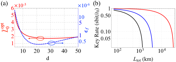
Figure S2: (a). Optimized spacing $\tilde{L}_{0,opt}$ (red) and associated bit-flip error rate per transmission $\epsilon_{f}$ (blue) with $\gamma=0.005$. (b). Optimized secure key rate with $\eta=99.4\%$ (black), $99.5\%$ (blue) and $99.6\%$ (red).