A Time-Dependent Wave-Thermoelastic Solid Interaction
This paper is dedicated to Wolfgang L. Wendland
on the occasion of his 80th birthday.)
Abstract
This paper presents a combined field and boundary integral equation method for solving the time-dependent scattering problem of a thermoelastic body immersed in a compressible, inviscid and homogeneous fluid. The approach here is a generalization of the coupling procedure employed by the authors for the treatment of the time-dependent fluid-structure interaction problem. Using an integral representation of the solution in the infinite exterior domain occupied by the fluid, the problem is reduced to one defined only over the finite region occupied by the solid, with nonlocal boundary conditions. The nonlocal boundary problem is analyzed with Lubich’s approach for time-dependent boundary integral equations. Existence and uniqueness results are established in terms of time-domain data with the aid of Laplace-domain techniques. Galerkin semi-discretization approximations are derived and error estimates are obtained. A full discretization based on the Convolution Quadrature method is also outlined. Some numerical experiments in 2D are also included in order to demonstrate the accuracy and efficiency of the procedure.
Key words: Fluid-structure interaction, Coupling BEM-FEM, Kirchhoff representation formula, Retarded potential, Time-domain boundary integral equation, Variational formulation, Wave scattering, Convolution quadrature.
Mathematics Subject Classifications: 35J20, 35L05, 45P05, 65N30, 65N38. ›
1 Introduction
The mathematical study of the thermodynamic response of a linearly elastic solid to mechanical strain dates back at least to Duhamel’s 1837 pioneering work [10] on thermoelastic materials where he proposed the constitutive relation linking the temperature variations and elastic strains with the thermoelastic stress now known as Duhamel-Neumann law [7, 32].
Kupradze’s encyclopedic works [23] can be considered the standard reference for a modern mathematical treatment of the purely thermoelastic problem. The dynamic problem is dealt with in more recent works like [34, 37] where the matrix of fundamental solutions for the dynamic equations is revisited, while [20, 21] provide generalized Kirchhoff-type formulas for thermoelastic solids.
In the case of the scattering of thermoelastic waves, major theoretical contributions have been made by Çakoni and Dassios in [6]. The unique solvability of a boundary integral formulation is established in [5] and the interaction of elastic and thermoelastic waves is explored for homogeneous materials in [8]. The study of time-harmonic interaction between a scalar field and a thermoelastic solid has been the subject of works like [27] where the interface is taken to be a plane, or [26, 22] where time-harmonic scattering by bounded obstacles is considered.
In this paper, we present a combined field and boundary integral method for a time-dependent fluid-thermoelastic solid interaction problem. The approach here is a generalization of the method employed by the authors for treating time-dependent fluid -structure interaction problems in [18, 17]. The present communication is an improvement over those previous efforts in the sense that it considers a more general constitutive law that accounts for the coupling between elastic and thermal effects. To our knowledge no attempt has been made to investigate with rigorous justifications the time-dependent acoustic scattering by a thermoelastic obstacle.
The setting is introduced in Section 2, along with the physical assumptions and the constitutive relation under consideration leading to the time-domain system of governing equations. The problem is then recast in Section 3 where the Laplace domain system is transformed into an equivalent integro-differential non-local problem that will be formulated variationally for discretization later on. The question of existence and uniqueness of the solutions to the non-local problem is dealt with on Section 4. The error analysis of the proposed discretization is addressed in Section 5, where semi-discrete error estimates for spatial discretization are provided.
The final Section 6 discusses the computational considerations related to the numerical solution of the discrete problem. A full discretization using Convolution Quadrature (CQ) in time is outlined and the coupling of boundary and finite elements for the spatial discretization is discussed. Convergence experiments in 2D are performed for test problems in both frequency and time domains as a demonstration of the applicability of the formulation which remains valid also in 3D. For time discretization both second order backward differentiation formula (BDF2) and Trapezoidal Rule CQ are used, providing evidence that the approximation is stable and of second order globally. Time-domain illustrative experiments using the proposed formulation are included.
In closing, we remark that for homogeneous thermoelastic solid medium, a pure boundary integral equation formulation may be adapted as in the fluid-structure interaction problem [17]. We will pursue these investigations in a separate communication.
2 Formulation of the problem
Consider a thermoelastic solid with constant density in an undeformed reference configuration and at thermal equilibrium at temperature . Under the action of external forces the body will be subject to internal stresses that will induce local variations of temperature. Reciprocally, if a heat source induces a change in temperature, the body will react by dilating or contracting and this will create internal stresses and deformations. We will denote by the elastic deformation with respect to the reference configuration and by the variation of temperature with respect to the equilibrium temperature. In the classical linear theory [23, 24], the coupling between the mechanic strain and the thermal gradient is modeled by the Duhamel-Neumann law which defines the thermoelastic stress and the thermoelastic heat flux (also known as free energy) as functions of the elastic displacement and the variation in temperature by
In the previous expressions
is the elastic strain tensor, is the identity matrix, is the thermal diffusivity coefficient, which from physical principles [14] is required to be positive, is the product of the volumetric thermal expansion coefficient and the bulk modulus of the material, and is given by the relation
Here the volumetric heat capacity is the ratio between the thermal diffusivity and the thermal conductivity, and it can also be expressed as the product of the mass density and the specific heat capacity. For the case of homogeneous isotropic material that we are considering, the elastic stiffness tensor is given by
where the constants and are Lamé’s second parameter and the shear modulus respectively, and is Kronecker’s delta.
We are concerned with a time-dependent direct scattering problem in fluid-thermoelastic solid interaction, which can be simply described as follows: an acoustic wave propagates in a fluid domain of infinite extent in which a bounded thermoelastic body is immersed. Throughout the paper, we let be the bounded domain in occupied by the thermoelastic body with a Lipschitz boundary and we let be its exterior, occupied by a compressible fluid. The problem is then to determine the scattered velocity potential in the fluid domain, the deformation of the solid and the variation of the temperature in the obstacle. It is assumed that .
The governing equations of the displacement field and temperature field are the thermo-elastodynamic equations:
| (2.1) | |||||||
| (2.2) |
where is a given positive final time, and as usual the symbol is the Lamé operator defined by
We remark that if the thermal effect is neglected () Duhamel-Neumann’s law reduces to the usual expression for Hooke’s law of the classical theory for an arbitrary isotropic medium (see, e.g. [7, 23]). In the thermoelastic medium, the given physical constants , are assumed to satisfy the inequalities:
In the fluid domain , we consider a barotropic and irrotational flow of an inviscid and compressible fluid with density as in [18]. The formulation can be presented in terms of a scalar potential such that the scattered velocity field and the pressure are given by
Then we arrive at the wave equation
| (2.3) |
where is the sound speed.
On the interface between the solid and the fluid we have the transmission conditions
| (2.4a) | ||||||
| (2.4b) | ||||||
| (2.4c) | ||||||
where is the exterior unit normal to , and denotes the given incident field, which is assumed to be supported away from at . Here and in the sequel, we adopt the notation that denotes the limit of the function on from respectively. Regarding the transmission conditions we remark that from the physical point of view, equation (2.4a) enforces the equilibrium of pressure at the solid-fluid interface, the condition (2.4b) expresses the continuity of the normal component of the velocity field, and (2.4c) refers to a thermally insulated body. We assume the causal initial conditions
| (2.5a) | ||||
| (2.5b) | ||||
We will study the the time-dependent scattering problem consisting of the partial differential equations (2.1)-(2.3) together with the transmission conditions (2.4a)-(2.4c) and the homogeneous initial conditions (2.5a)-(2.5b).
3 Reduction to a nonlocal problem
In order to apply Lubich’s approach as in the case of fluid-structure interaction [18, 17], we first need to transform the initial-boundary transmission problem (2.1)-(2.4c) in the Laplace domain. Then we reduce the corresponding problem to a nonlocal boundary value problem. We begin with the Laplace transform for a restricted class of distributions. Let be a Banach space and denote the Schwartz class of functions. We say that is a causal tempered distribution with values in if it is a continuous linear map such that
For such a distribution and
the Laplace transform of can be defined in a natural way by
where the integral must be understood in the sense of Bochner [35]. We remark that the Laplace transform can be defined for a much broader class of distributions [4, 9], but this restricted class suffices for the current application.
Let then
Then the initial-boundary transmission problem consisting of (2.1) - (2.4c) in the Laplace transformed domain becomes the following transmission boundary value problem:
| (3.1a) | ||||||
| (3.1b) | ||||||
| (3.1c) | ||||||
| (3.1d) | ||||||
| (3.1e) | ||||||
| (3.1f) | ||||||
We remark that (3.1) is an exterior scattering problem for which normally a radiation condition is needed in order to guarantee the uniqueness of the solution. However, in the present case no additional radiation condition is required and global behavior at infinity suffices.
To derive a proper nonlocal boundary problem, as usual, we begin via Green’s third identity with the representation of the solutions of (3.1c) in the form:
| (3.2) |
where and are the Cauchy data for in (3.1c) and and are the simple-layer and double-layer potentials, respectively defined by
| (3.3) | ||||||
| (3.4) |
Here
is the fundamental solution of the operator in (3.1c). By standard arguments in potential theory, we have the relations for the the Cauchy data and :
| (3.5) |
Here and are the four basic boundary integral operators familiar from potential theory [19] such that
By using the transmission condition (3.1e), we obtain from the second boundary integral equation in (3.5),
| (3.6) |
while the first boundary integral equation in (3.5) is simply
| (3.7) |
With the Cauchy data and as new unknowns, the partial differential equation (3.1c) in may be eliminated. This leads to a nonlocal boundary value problem in for the unknowns satisfying the partial differential equations (3.1a), (3.1b), and the boundary integral equations (3.6), (3.7) together with the conditions (3.1d) and (3.1f) on .
Here and in the sequel let and denote trace operators of the functions and their normal derivatives from inside and outside , respectively. We will use the symbol interchangeably to denote the scalar, vector, or Frobenius inner products of functions defined on the open set , while the angled brackets will be reserved for pairings between elements of the trace space and its dual. All the forms will be kept linear and conjugation will be done explicitly when needed. Finally, the space should be understood as the Cartesian product of copies of the standard scalar Sobolev space endowed with the natural product norm.
Let us first consider the unknowns . Then multiplying (3.1a) by the testing function and integrating by parts, we obtain the weak formulation of (3.1a):
| (3.8) |
where is the bilinear form defined by
| (3.9) |
In terms of the transmission condition (3.1d), we obtain from (3.8)
| (3.10) |
Similarly, multiplying (3.1b) by the test function , integrating by parts and making use of the condition (3.1f), we have
| (3.11) |
with
| (3.12) |
Now let
be the operators associated to the bilinear forms (3.9) and (3.12), respectively. Then from (3.10), (3.12), (3.6), and (3.7), the nonlocal problem may be formulated as a system of operator equations: Given data find such that
| (3.13) |
In the above expression denotes the transpose (row) of the outward unit normal (column) to , and data is given by
| (3.14) |
We have made use of the product spaces:
(i. e., is the dual of ). Our aim is to show that equation (3.13) has a unique solution in . We will do this in the next section.
4 Existence and uniqueness results
Before considering the existence and uniqueness results, we first discuss the invertibility of the operator in (3.13). We begin with the definitions of the following energy norms:
| (4.1) | |||||
| (4.2) | |||||
| (4.3) |
For the complex Laplace parameter we will denote
and will make use of the following equivalence relations for the norms
| (4.4) | |||
| (4.5) | |||
| (4.6) |
which can be obtained from the inequalities:
We remark that the norms and are equivalent to and , respectively, and so is the energy norm equivalent to the norm of by the second Korn inequality [11].
For the invertibility of , let us introduce the diagonal matrix :
| (4.7) |
and consider the modified operator
| (4.8) |
It will be clear that in order to show the invertibility of it suffices to prove that of . By the Gaussian elimination procedure (as in [25]), a simple computation shows that can be decomposed in the form:
| (4.9) |
where
with .
Since both and are invertible, the invertibility of will imply that of , but as in the time-dependent fluid-structure interaction [18], the operator matrix is indeed invertible. In fact, it is not difficult to show that the operator matrix is strongly elliptic [19, 33] in the sense that
| (4.10) |
for all , where is a constant depending only on the physical parameters and on the geometry of , and is the matrix defined by
The action of amounts only for a rotation that reveals the elliptic nature of the original system. As such, the analyticity of is immaterial, since only the inverse Laplace transform of is sought for. As for the proof of (4.10), we will just point out that it is simple to show that
| (4.11) | |||||
Further details are omitted, since a similar proof will be repeated when we discuss the existence and uniqueness results for the solution of the nonlocal problem (3.13).
We now return to the solutions of the modified system of equations (4.8) from (3.13):
| (4.12) |
Suppose that is a solution of (4.12). Let
| (4.13) |
Then is the solution of the transmission problem:
| (4.14) |
satisfying the following jump relations across ,
First, from (4.14) we see that
| (4.15) | |||||
| (4.16) | |||||
| (4.17) | |||||
| (4.18) |
Since , this means that is a solution of the homogeneous Dirichlet problem for the partial differential equation (4.14) in . Hence by the uniqueness of the the solution, we obtain in . Consequently, we have
| (4.19) |
Next, we consider the variational formulation of the problem for equations (4.14) , (4.15) and (4.16) together with the boundary conditions (4.17) and (3.1f). We seek a solution
with the corresponding test functions in the same function space. To derive the variational equations, we should keep in mind that the variational formulation should be formulated not in terms of the Cauchy data and directly, but only through the jumps and as indicated.
Let , we introduce the bilinear form
and its associated operator
Note that in these definitions the domain of integration is indicated explicitly. Using this notation we can use the first Green formula for equation (4.14) and condition (4.17) to obtain
| (4.20) |
Together with the weak formulations of (4.15) and (4.16), we arrive at the following variational formulation: Find satisfying
| (4.21) | |||||
We remark that by construction, it can be shown that as in [35] this variational problem is equivalent to the transmission problem defined by (4.14), (4.15), (4.16), and (4.17). The latter is equivalent to the nonlocal problem defined by (4.12), which is equivalent to (3.13). Consequently, the variational problem (4.21) is equivalent to the nonlocal problem (3.13). Hence for the existence of the solution of (3.13), it is sufficient to show the existence of the solution of (4.21).
We have the following basic results.
Theorem 4.1.
The variational problem (4.21) has a unique solution . Moreover, the following estimate holds:
| (4.22) |
where is a constant depending only on the physical parameters .
Proof.
Starting with the system (4.21), a simple computation shows that
| (4.23) |
On the other hand, it is not hard to verify that
| (4.24) | ||||
| (4.25) | ||||
| (4.26) |
Therefore, combining (4.24) - (4.26), substituting into (4.23) and recalling that , it follows that
However, from the definition we see that the left hand side of this expression satisfies
Consequently, we have the estimate
| (4.27) |
where is a constant depending only on the physical parameters . In deriving the estimate (4.27), we have tacitly applied the relations (4.4), (4.5) and (4.6). ∎
As we will see the estimate (4.27) will lead us to show the invertibility of the operator in (3.13) (or (4.12) rather). In fact, the following result holds for the operator of (4.12).
Theorem 4.2.
Let
Then is invertible . Moreover, we have the estimate:
| (4.28) |
where is a constant independent of and .
Proof.
It was pointed out in (4.19) that
Then we have the estimates (see, e.g. [18]):
| (4.29) |
Similarly, an application of Bamberger and Ha-Duong’s optimal lifting [1, 2] leads to the estimate
A detailed proof of this inequality can be found in [35, Proposition 2.5.2]. Thus, we can conclude that
| (4.30) |
From (4.29) and (4.30), we obtain the estimates
| (4.31) |
As a consequence of (4.22), it follows that
A simple manipulation shows that the left hand side of the previous expression is such that
which implies that
with constant independent of and . ∎
We remark that in view of (3.2), we see that and are solutions of the system
| (4.32) |
With the properties of solutions available in the transformed domains, we are now in a position to estimate the corresponding properties of solutions in the time domain based on Lubich’s Convolution Quadrature [30], introduced in the early 90’s for treating time-dependent boundary integral equations of convolution type.
An essential feature of this approach is that estimates of properties of solutions in the time domain are obtained without the need for applying the inverse Laplace transform. Instead, the crucial result described on Proposition 4.3 below is employed to retrieve time domain estimates from those obtained in the Laplace domain.
Before presenting the aforementioned result we must introduce some notation. For Banach spaces and , let denote the set of bounded linear operators from to . We say that an analytic function is an element of the class of symbols if there exist and such that
where is a non-increasing function such that
In order to make the statement of the time-domain estimates more compact, we will make use of the regularity spaces
| (4.33) |
where denotes a Banach space.
Remark: The proof of this result can be found in full detail in [35, Proposition 3.2.2].
As an immediate consequence of this result, we see from Theorem 4.2 that . Moreover, and and we thus have the estimate:
Theorem 4.4.
Let belong to . Then
and there exists depending only on the geometry such that
| (4.34) |
Similarly, in view of Theorem 4.1, applying Proposition 4.3 with to the elastic, thermal, and potential fields leads to:
Theorem 4.5.
Let and
Then belongs to and there holds the estimate
| (4.35) |
for some constant .
5 Semi-discrete error estimates
In this section, we discuss the results concerning the discretization of (3.13). We begin with the Galerkin semi discretization in space of the system of equations. Let
be families of finite dimensional subspaces. We say is a Galerkin solution of (3.13) if it satisfies the Galerkin equations:
| (5.1) |
for all . Again, we multiply (5.1) by the diagonal matrix in (4.7) and consider the Galerkin equations for the modified equation (4.12):
| (5.2) |
for all . Solutions of Galerkin equations of (5.2) can be established in the same manner as the exact solutions of the system (4.21). We will not repeat the process and consider only the error estimates here.
We note that if is a Galerkin solution of (5.2), then
| (5.3) |
satisfies
| (5.4) | ||||||
Now set
Here and in the sequel, the upper script ∘ will be used to denote the annihilator (or polar set) of a given Banach space. In this particular case,
Applying Green’s formula to (5.4), we obtain for ,
| (5.5) |
As a consequence, we see that satisfies the variational equations
| (5.6) | ||||||
For the error estimate, we need to compare with the exact solution of the transmission problem. The exact solution satisfies the variational equation (4.21), which can be put in the same form as (5.6) by choosing test functions in the discrete subspaces. This implies that
| (5.7) | ||||||
The significance of (5.7) is that it indicates that the Galerkin solutions are the best possible approximations of the exact solution in the finite dimensional subspaces with respect to the inner products defined by the underlying bilinear forms. However, it is worth emphasizing that the errors and do not belong to the discrete function spaces. In order to justify (5.7) as a proper variational formulation, we will make use of the spaces of constants and of infinitesimal rigid motions
| (5.8) | ||||
| (5.9) |
which in what follows will always be assumed to be contained on the discrete subspaces and respectively. We now define the elliptic projection on displacement fields
| (5.10) | |||||
This projection is well defined thanks to Korn’s second inequality and can be alternatively introduced as the orthogonal projection onto with respect to the non-standard (but equivalent) inner product in
where is the orthogonal projection onto . This implies that the approximation error is equivalent to the best approximation error in by elements of . Similarly, we can introduce a projection on the discrete scalar fields
| (5.11) | |||||
Note that the reason to introduce these projections is to avoid having additional mass terms arising from the full Sobolev norm in the associated error equations.
In terms of the elliptic projection , we can define
so that the error function can be decomposed as
As a consequence
We may decompose the error in a similar manner by letting
so that
Finally, we define
This leads to the variational formulation for the error functions .
Theorem 5.1.
The error functions satisfy the variational formulation
Where the bilinear form is defined by
| (5.12) |
and the functional is given by
| (5.13) |
Proof.
The bilinear form follows easily from the left hand side of (5.6) replacing by and taking special care of the term .
Following arguments similar as those employed in the proof of Theorem 4.1, we can obtain the error estimate. In the following, for simplicity, let
Theorem 5.2.
For , there holds the error estimate:
| (5.14) |
where the constant depends only on the geometry, and physical parameters.
Proof.
It is easy to see from the definition of the bilinear form in (5.12) that there is a constant C depending only on the geometry and physical parameters such that
| (5.15) |
We also need the estimate for the functional
| (5.16) |
For , we pick a lifting such that . Thus,
Since , it follows from equations (4.24)-(4.26) that
And the result follows from this relation and the observation that
∎
We are now in the position to establish the following result.
Corollary 5.3.
Regarding the proof of this result, we would only like to point out that the estimate (5.17a) follows from a combined application of (5.14) in Theorem 5.2, and (4.29) by making use of the jump condition . On the other hand, in order to establish the estimate (5.17b), one has to recall that and therefore an application of (4.30) combined with (5.14) yields the desired inequality.
Corollary 5.3 has the awkward aspect of being an error estimate where part of the right-hand side (the terms and ) does not converge to zero. We now clarify why this is not so. Consider the best approximation operators
If we create data for the problem so that the exact solution is , then the associated numerical solution will be the exact solution and there will be no error in the method. Therefore, by linearity, we can use as exact solution in Corollary 5.3 and the numerical solution will be . Consequently, we can substitute by in the right-hand-side of (5.17a)-(5.17b).
If we now apply Proposition 4.3 to Corollary 5.3, we may obtain the following estimates in the time domain.
Corollary 5.4.
If the exact solution quadruple satisfies
then
is causal and for
where
6 Computational Aspects
6.1 Convolution Quadrature
We present a very brief description of the procedure used to obtain a full discretization using multistep-based Convolution Quadrature. The process was devised by Christian Lubich [28, 29], and was designed employed originally for treating constitutional boundary integral equations [30, 31] and in recent times has become a very powerful tool for the discretization of time domain problems. The present description is by no means comprehensive and is provided only for the sake of completeness, the interested reader is refereed to [15], where very detailed descriptions of the theory and implementation for both multi-step and multi-stage flavors of Convolution Quadrature are given.
Suppose that
and let
be the basis functions of the spaces , and , respectively. We choose a time-step and let us consider the uniform grid in time for We define to be the stiffness matrix of equation (5.2). is a matrix valued function of whose structure is depicted in Figure 1.
The data are sampled in time and tested to define vectors :
where in Theorem 4.4. The CQ discretization of (5.2) starts with the Taylor expansion
| (6.1) |
where characterizes the underlying k- multistep method, and is, therefore, usually referred to as the characteristic function of the linear multistep method.
For the discretization of (5.2), we seek the sequence of vectors given by the recurrence:
| (6.2) |
The coefficients can be computed by means of Cauchy’s integral formula
For implementation purposes, the integration contour is taken to be a circle with radius dependent on the number of terms in the expansion and the specific value of the computer’s machine epsilon [15]. This choice of contour allows for fast and accurate computation of the coefficients exploiting the properties of the trapezoidal rule and the Fast Fourier Transform.
6.2 A combined approach for time evolution
The linear system arising from the discretization and depicted in Figure 1 can be thought of as having the block structure
where the sparse Finite Element block
contains mass and stiffness matrices as well as first order terms related to the elastic and thermal unknowns. The boundary element block contains the Galerkin discretization of the operators of the acoustic Calderón calculus and the coupling trace matrix is the discretization of the bilinear form arising from the duality pairing .
Even if a CQ approach can be applied to the entire system using the expansion (6.1) on the global matrix and solving the resulting linear system (5.14), it is a common practice to decouple the computations of the finite element and boundary element unknowns via a Schur complement strategy. The decoupled Boundary Element unknowns are then evolved in time using CQ (via (6.1) and (5.14)), while the same underlying multistep scheme is used for the Finite Element unknowns. This process was first described in [3] and is explained in detail in [16], where it is used in the context of for purely acoustic waves.
6.3 Numerical Experiments
In order to test numerically the formulations of the previous sections, computational convergence studies were performed in both frequency and time domains for 2D test problems. Moreover, we explore numerically the case when the Lamé parameters or the thermal diffusivity and expansion are non constant tensors. We emphasize that the goal of the computations presented here is mainly to provide a proof of concept of the suggested discretization and to highlight the fact that the discretization can be readily implemented with only minor additions to existing code. The previous analysis remains valid in 3D and the implementation of the discretization in that case can be done following completely analogous steps.
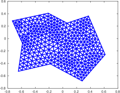
The computational domain. For the convergence studies, the interior domain where the thermoelastic equations were imposed was the polygon depicted in Figure 2. The domain was generated and meshed using Matlab’s pdetool. All the mesh refinements were done using the refinement capabilities of the pde toolbox.
Approximation errors. As a measurement of the accuracy of the approximations, the difference between the manufactured solution and the approximate Finite Element solutions was measured in the and norms for the elastic and thermal variables and . For the acoustic unknown , the approximate solution was sampled in 25 randomly placed points in and the maximum absolute difference with the exact solution was taken as a measure of the error. In the time domain experiments this measurements were done for the a final time .
Physical parameters. The following values of the physical parameters are functions only of space and were used equally for both series of experiments. They are chosen for validation and expository purposes only and do not correspond with any relevant physical material. For the entries of the tensors we make use of the symmetries and of Voigt’s notation [13] to shorten the subscripts.
-
1.
Density of the elastic solid and Lamé parameters
(6.3) -
2.
Thermal expansion tensor :
(6.4) -
3.
Thermal diffusivity tensor :
(6.5) -
4.
The components of the tensor were chose to be:
(6.6)
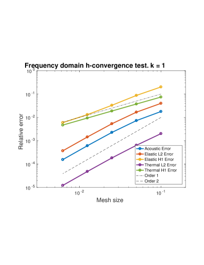
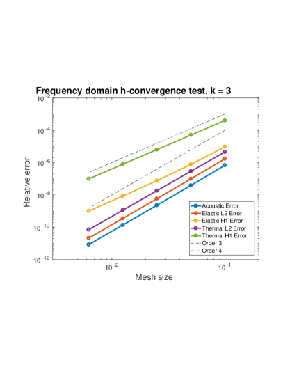
Convergence studies in the frequency domain. We first verify the results in the frequency domain. We proceed by the method of manufactured solutions using the functions
together with the parameters defined in (6.3) through (6.6). Right-hand side load vectors and boundary conditions were constructed accordingly.
For the numerical experiments, Lagrangian finite elements were used for the elastic and thermal unknowns, while Galerkin continuous/discontinuous Boundary Elements were used for the acoustic potential . Convergence studies for spatial refinements with a fixed polynomial degree (h-convergence) and increasing degree of polynomial approximation with a fixed mesh size (p-convergence) were performed for . The results of the mesh-refinement experiments are shown in Tables 2, 3, and 4. The table 5 contains the results for a fixed mesh with increasing polynomial degree for the basis functions. The convergence plots for all the simulations are displayed in Figure 3.
Convergence studies in the time domain. In a way analogous to the previous section, the numerical experiments were carried out using the physical parameters and coefficients given in (6.3) through (6.6) and with manufactured solutions using the functions
| where is the Laplace transform, the time factor is given by | |||||
| (6.8a) | |||||
and is the approximation to Heaviside’s step function
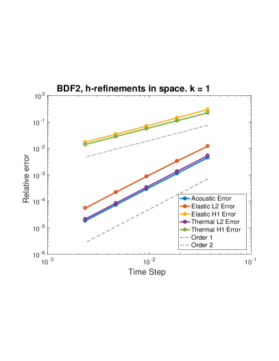
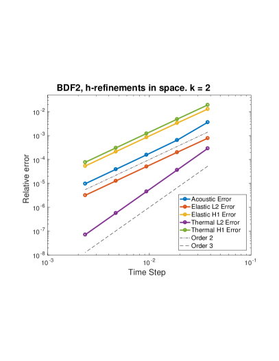
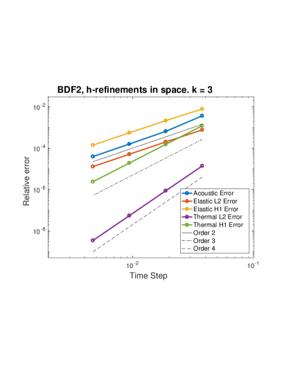
Two kinds of experiments were carried out using the same geometry as in the frequency domain. On the one hand, for a spatial discretization with fixed polynomial degree, successive dyadic refinements in both mesh size and time step were carried out (h-refinement). The experiment was repeated for polynomial degrees , and 3 starting with with a spatial mesh with parameter and time step .
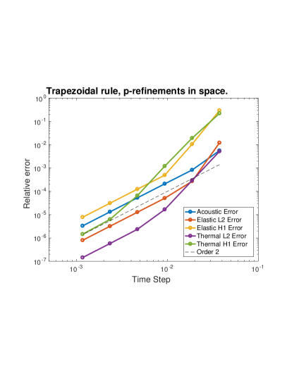
The second experiment corresponds to p-refinements in space and consisted in using a fixed spatial mesh, starting with a polynomial discretization of degree in space and a time step . With every successive dyadic refinement of , the degree of the polynomial interpolant was increased by one. The initial mesh size of corresponds to the second level of refinement used for the h-refinement experiments. This space-time refinement strategies highlight the global order of convergence of the method, which is expected to be asymptotically limited by the order of the multi-step scheme used for time discretization.
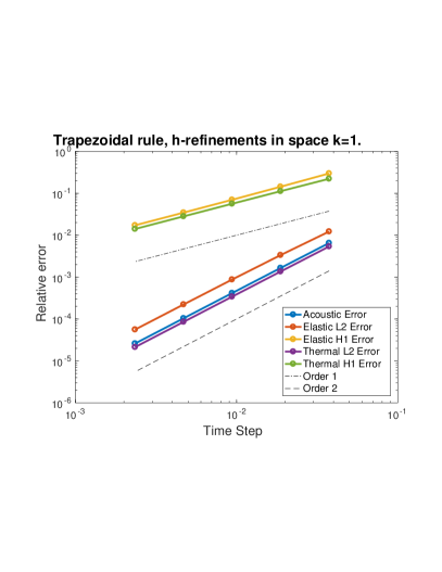
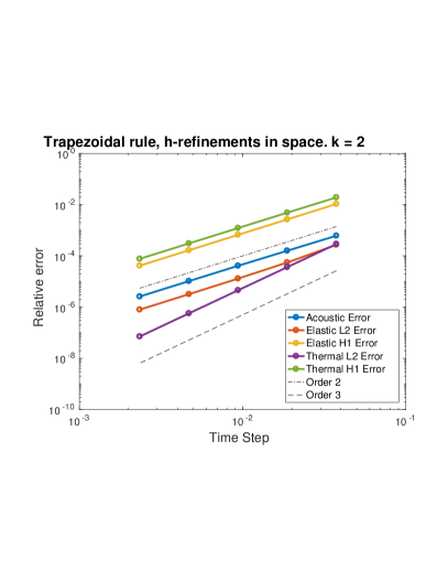
Both strategies were tried for BDF2 and Trapezoidal Rule based time discretizations. The results for the studies using BDF2 are shown in Tables 6, 7, 8 (h-refinement), and 9 (p-refinement). These results are summarized in the convergence plot of Figure 4. Similarly, the results for the experiments using Trapezoidal Rule time stepping are shown in Tables 10, 11, 12 (h-refinement), and 13 (p-refinement), all condensed on the convergence plots shown in Figure 5.
Depending on the refinement strategy, the number of degrees of freedom required to approximate to the system increases quickly, especially for h-refinements with higher order polynomial basis. Table 1 shows the number of unknowns associated to a single scalar FEM function represented in the grid shown in Figure 2. The increase in computational requirements imposed by h-refinement makes some asymptotic properties of the scheme difficult to observe following this strategy.
In particular, the smoothing properties of the parabolic part of the system introduce superconvergent behavior on the thermal unknowns during the pre-asymptotic regime. As can be seen in the p-refinement experiments (c.f. Figures 4 and 5, bottom right) the convergence stabilizes to the predicted rate for relatively small time step, after five refinement levels. The number of spatial degrees of freedom required to achieve such a discretization level by h-refinements causes the true convergence rate to be observable only using a p-refinement strategy.
Growth in FEM DOF Refinement Level Refinement Strategy 1 2 3 4 5 6 h-refinement, 108 394 1503 5869 23193 92209 h-refinement, 394 1503 5869 23193 92209 161225 h-refinement, 859 3328 13099 51973 207049 413537 p-refinement 108 394 859 1503 2326 3328
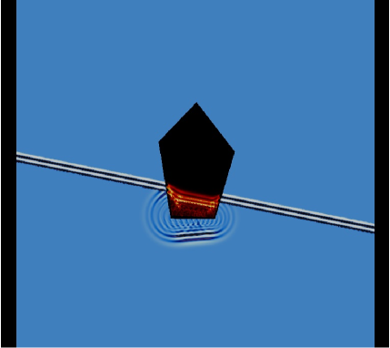
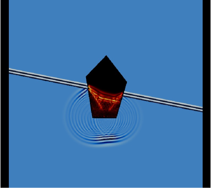
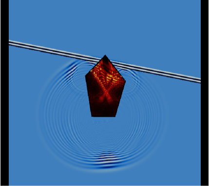
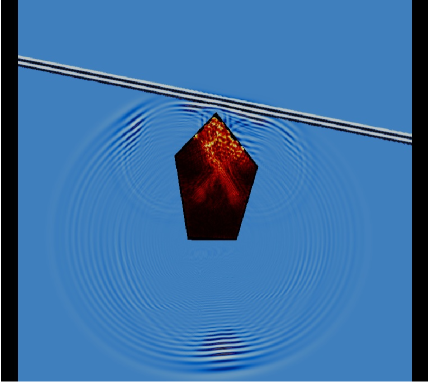
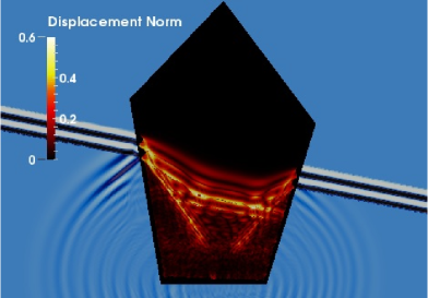
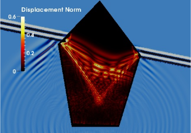
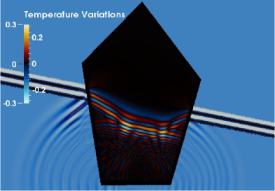
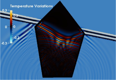
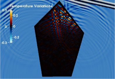
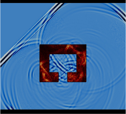
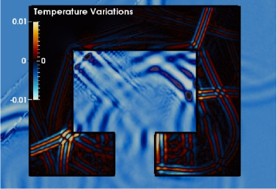
Examples. We now present a couple of illustrative examples in 2D. The first example shows the interaction between the plane wave
and a pentagonal scatterer with mass density given by
The values of the elastic parameters, thermic diffusivity , thermoelastic expansion tensors and were the same as those used for the convergence experiments in the previous paragraphs and given in equations (6.3)-(6.6). The simulation used Lagrangian finite elements on a grid with mesh parameter and 36096 elements. The inherited boundary element grid had 496 panels and a grid parameter of , and continuous/discontinuous Galerkin boundary elements were used. Trapezoidal rule-based discretization was applied in time with a time step . Some snapshots of the simulation are shown in Figures 6-8.
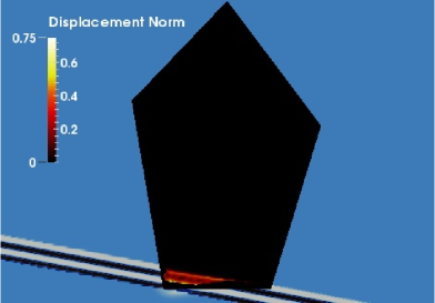
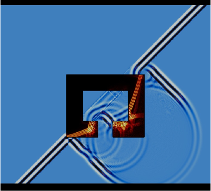
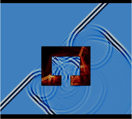
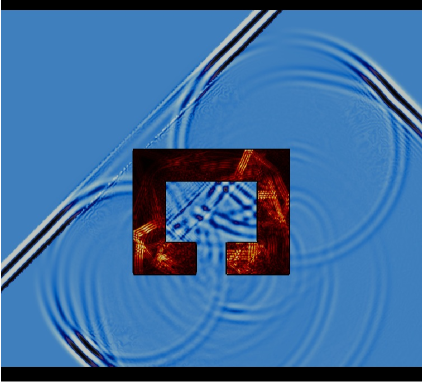
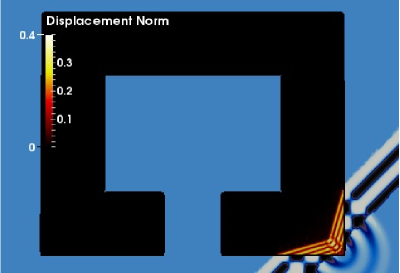
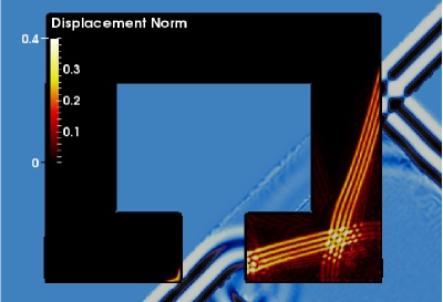
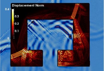
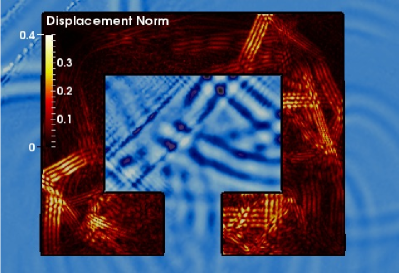
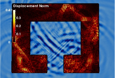
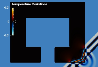
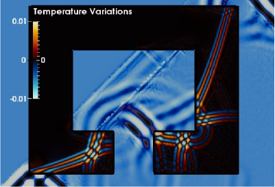
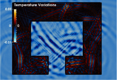
The second example is a trapping geometry with density and physical parameters given by (6.3)-(6.6). For this example Lagrangian elements were used on a grid with 2992 elements and mesh parameter , the acoustic equations were discretized with continuous/discontinuous Galerkin boundary elements on a mesh with 236 panels and mesh parameter . For time discretization trapezoidal rule-based CQ was used with a time step size of . Figures 9-11 show snapshots of the acoustic, elastic and temperature fields.
Acknowledgements.
The authors would like to thank the referees for their detailed comments and suggestions, which greatly improved the quality of this communication.
In respectful memory of Prof. Richard Weinacht.
References
- [1] A. Bamberger and T. Ha-Duong. Formulation Variationnelle Espace-Temps pour le Calcul par Potentiel Retardé de la Diffraction of d’une Onde Acoustique (I) Math. Meth. Appl.Sci, 8(3): 405–435, 1986.
- [2] A. Bamberger and T. Ha-Duong. Formulation Variationnelle pour le Calcul de la Diffraction of d’une Onde Acoustique par une Surface Rigide Math. Meth. Appl.Sci, 8(4): 598–608, 1986.
- [3] L. Banjai and S. Sauter. Rapid solution of the wave equation in unbounded domains. SIAM J. Numer. Anal., 47(1):227–249, 2008/09.
- [4] E. J. Beltrami and M. R. Wohlers. Distributions and the Boundary Values of Analytic Functions Academic Press, 1966.
- [5] F. Çakoni. Boundary integral method for thermoelastic screen scattering problem in . Mathematical Methods in the Applied Sciences, 23(5): 441–466. John Wiley & Sons, Ltd., 2000.
- [6] F. Çakoni and G. Dassios. The coated thermoelastic body within a low-frequency elastodynamic field, Int. J. Eng. Sci. 36, 1815–1838, 1998.
- [7] D. Carlson. Linear thermoelasticity. In Encyclopedia of Physics, Vol. VIa/2, C. Truesdell, ed., Springer-Verlag, New York, 1972.
- [8] G. Dassios and V. Kostopoulos. Scattering of elastic waves by a small thermoelastic body. Int. J. Eng. Sci., 32(10): 1593–1603, 1994.
- [9] R. Dautray and J.-L. Lions. Mathematical analysis and numerical methods for science and technology. Vol. 5. Springer-Verlag, Berlin, 1992. Evolution problems. I, With the collaboration of Michel Artola, Michel Cessenat and Hélène Lanchon, Translated from the French by Alan Craig.
- [10] Duhamel, J.-M.-C. Second mémoire sur les phénomènes thermo-mécaniques. J. de l’École Polytechnique, Tome 15, cahier 25, pp. 1–-57, 1837.
- [11] G. Fichera. Existence theorems in elasticity theory. 347–389, Volume 2 Handbuch der Physik. Springer, 1972.
- [12] T. Ha-Duong. On the transient acoustic scattering by a flat object. Japan Journal of Applied Mathematics, Vol. 7, No. 3: 489–513, 1990.
- [13] M.E. Gurtin. The linear theory of elasticity, Mechanics of Solids II, Encyclopedia of Physics, Springer, Berlin, 1972.
- [14] D.W. Hahn and M.N. Ozisik. Heat Conduction. Wiley, 2012.
- [15] M. Hassell and F.-J. Sayas. Convolution Quadrature for Wave Simulations. Springer SEMA-SIMAI Lecture Notes in Mathematics, 2016. To appear.
- [16] M. E. Hassell and F.-J. Sayas. A fully discrete BEM-FEM scheme for transient acoustic waves. Comput. Methods Appl. Mech. Engrg., 309:106 – 130, 2016.
- [17] George C. Hsiao, Tonatiuh Sánchez-Vizuet, and Francisco-Javier Sayas. Boundary and coupled boundary-finite element methods for transient wave-structure interaction. IMA Journal of Numerical Analysis, 37(1):237–265, 2016.
- [18] G.C. Hsiao, J.F. Sayas and R.J. Weinacht. A Time-Dependent Fluid-Structure Interaction. Math. Meth. Appl. Sci., DOI: 10.1002/sim.0000.
- [19] G.C. Hsiao and W.L. Wendland. Boundary Integral Equations, Applied Mathematical Sciences, 164 Springer, Berlin, 2008.
- [20] M. Jakubowska. Kirchhoff’s formula for thermoelastic solid. J. Therm. Stresses, 5(2): 127-144, 1982.
- [21] M. Jakubowska. Kirchhoff’s type formula in thermoelasticity with finite wave speeds. J. Therm. Stresses, 7(3–4): 259–283, 1984.
- [22] L. Jentsch and D. Natroshvili. Interaction between thermoelastic and scalar oscillation fields. Integr. Equat. Oper. Th., 28(3): 261–288, 1997.
- [23] V.D. Kupradze. Three-dimensional Problems of the Mathematical Theory of Elasticity and Thermoelasticity, North-Holland Series in Applied Mathematics and Mechanics, 164 North-Holland Publishing Company, Amsterdam, New York, Oxford, 1979.
- [24] L.D. Landau and E.M. Lifshitz and A.M. Kosevich and L.P. Pitaevskiĭ. Theory of Elasticity, volume 7 of the Course of theoretical physics. Butterworth-Heinemann, 1986.
- [25] A. R. Laliena and F.-J. Sayas. Theoretical aspects of the application of convolution quadrature to scattering off acoustic waves. Numer. Math. , 112: 637–678, 2009.
- [26] W.H. Lin and A.C. and Raptis. Thermoviscous effects on acoustic scattering by thermoelastic solid cylinders and spheres. J. Acoust. Soc. Am. 74(5): 1542–1554, 1983.
- [27] A.A. Lopat’ev. Effect of thermoelastic scattering in a liquid and solid body on the reflection of harmonic waves from a plane boundary of separation. Soviet Applied Mechanics, 15(1): 79–82, 1979.
- [28] Ch. Lubich. Convolution quadrature and discretized operational calculus, I. Numer. Math., 52(2): 129–145, 1988.
- [29] Ch. Lubich . Convolution quadrature and discretized operational calculus, II. Numer. Math., 52(4): 413–425, 1988.
- [30] Ch. Lubich . On the multistep time discretization of linear initial-boundary value problems and their boundary integral equations. Numer. Math., 67(3): 365–389, 1994.
- [31] Ch. Lubich and R. Schneider. Time discretization of parabolic boundary integral equations. Numer. Math., 63(4): 455–481, 1992.
- [32] G. Maugin. Continuum mechanics through the eighteenth and nineteenth centuries. Solid Mechanics and its Applications, 214. Springer, Cham, 2014.
- [33] C. Miranda. Partial Differential Equations of Elliptic Type, Springer, Berlin, 1970.
- [34] N. Ortner and P. Wagner. On the fundamental solution of the operator of dynamic linear thermoelasticity. J. Math. Anal. Appl., 170(2): 524–550, 1992.
- [35] F.-J. Sayas. Retarded potentials and time domain boundary integral equations: a road-map. Computational Mathematics, 50. Springer, 2016.
- [36] T. Sánchez-Vizuet. Integral and coupled integral-volume methods for transient problems in wave-structure interaction. PhD. Thesis. Department of Mathematical Sciences, University of Delaware, May, 2016.
- [37] P. Wagner, P. Fundamental Matrix of the system of dynamic linear thermoelasticity. J. Therm. Stresses, 17(4): 592–565, 1994.
e.c.r. e.c.r. e.c.r. e.c.r. e.c.r. 1 E-1 1.787 E-2 — 3.999 E-2 — 2.015 E-3 — 2.011 E-1 — 7.430 E-2 — 5.016 E-2 7.292 E-3 1.293 1.675 E-2 1.255 6.397 E-4 1.656 8.733 E-2 1.203 3.746 E-2 0.988 2.508 E-2 2.272 E-3 1.683 5.344 E-3 1.648 1.837 E-4 1.799 3.297 E-2 1.405 1.876 E-2 0.976 1.254 E-2 6.099 E-4 1.897 1.447 E-3 1.885 4.824 E-5 1.929 1.314 E-2 1.327 9.383 E-3 0.996 6.27 E-3 1.556 E-4 1.971 3.703 E-4 1.966 1.223 E-4 1.980 5.961 E-3 1.141 4.692 E-3 1.000
e.c.r. e.c.r. e.c.r. e.c.r. e.c.r. 1 E-1 7.926 E-5 — 1.284 E-4 — 9.742 E-5 — 3.514 E-3 — 6.446 E-3 — 5.016 E-2 6.676 E-6 3.570 1.181 E-5 3.442 1.214 E-5 3.004 8.708 E-4 2.013 1.630 E-3 1.983 2.508 E-2 5.590 E-7 3.578 1.207 E-6 3.290 1.517 E-6 3.000 2.172 E-4 2.003 4.093 E-4 1.993 1.254 E-2 4.630 E-8 3.594 1.331 E-7 3.181 1.897 E-7 2.999 5.426 E-5 2.001 5.426 E-5 1.997 6.27 E-3 3.793 E-9 3.609 1.550 E-8 3.103 2.373 E-8 2.999 1.356 E-8 2.001 2.566 E-5 1.999
e.c.r. e.c.r. e.c.r. e.c.r. e.c.r. 1 E-1 6.847 E-7 — 1.726 E-6 — 4.564 E-6 — 9.540 E-6 — 4.018 E-4 — 5.016 E-2 3.869 E-8 4.145 9.804 E-8 4.138 2.886 E-7 3.983 7.701 E-7 3.631 5.044 E-5 2.994 2.508 E-2 2.279 E-9 4.085 5.794 E-9 4.081 1.810 E-8 3.995 7.600 E-8 3.341 6.312 E-6 2.998 1.254 E-2 1.375 E-10 4.051 3.502 E-10 4.048 1.132 E-9 3.999 8.504 E-9 3.160 7.892 E-7 3.000 6.27 E-3 8.468 E-12 4.021 2.141 E-11 4.032 7.076 E-11 4.000 1.011 E-9 3.072 9.866 E-8 3.000
Ndof (degree) e.c.r. e.c.r. e.c.r. e.c.r. e.c.r. 108 (1) 1.787 E-2 — 3.999 E-2 — 2.015 E-3 — 2.011 E-1 — 7.430 E-2 — 394 (2) 7.926 E-5 — 1.284 E-4 — 9.742 E-5 — 3.514 E-3 — 6.446 E-3 — 859 (3) 6.848 E-7 — 1.726 E-6 — 4.564 E-6 — 9.540 E-6 — 4.018 E-4 — 1503 (4) 5.185 E-9 — 1.154 E-8 — 1.503 E-7 — 2.861 E-7 — 2.042 E-5 — 2326 (5) 1.241 E-10 — 3.533 E-10 — 5.814 E-9 — 9.008 E-9 — 8.133 E-7 —


BDF2. k=1 () e.c.r. e.c.r. e.c.r. e.c.r. e.c.r. 3.75 E-2 (1.000 E-1) 4.486 E-3 — 1.217 E-2 — 5.381 E-3 — 2.975 E-1 — 2.221 E-1 — 1.875 E-2 (5.016 E-2) 1.130 E-3 1.989 3.337 E-3 1.867 1.358 E-3 1.987 1.434 E-1 1.053 1.121 E-1 0.986 9.375 E-3 (2.508 E-2) 1.130 E-3 1.989 3.337 E-3 1.867 1.358 E-3 1.987 1.434 E-1 1.053 1.121 E-1 0.986 4.697 E-3 (1.254 E-2) 7.293 E-5 1.990 2.214 E-4 1.975 8.528 E-5 1.998 3.458 E-2 1.017 2.814 E-2 0.999 2.344 E-3 (6.270 E-3) 1.827 E-5 1.997 5.569 E-5 1.991 2.133 E-5 1.999 1.721 E-2 1.006 1.407 E-2 1.000
BDF2. k=2 () e.c.r. e.c.r. e.c.r. e.c.r. e.c.r. 3.75 E-2 (1.000 E-1) 3.624 E-3 — 7.798 E-4 — 2.917 E-4 — 1.297 E-2 — 1.934 E-2 — 1.875 E-2 (5.016 E-2) 6.471 E-4 2.486 2.004 E-4 1.960 3.640 E-5 3.002 3.370 E-3 1.944 4.890 E-3 1.983 9.375 E-3 (2.508 E-2) 1.571 E-4 2.043 5.062 E-5 1.985 4.550 E-6 3.000 8.524 E-4 1.983 1.228 E-3 1.993 4.697 E-3 (1.254 E-2) 3.891 E-5 2.013 1.271 E-5 1.994 5.692 E-7 2.999 2.137 E-4 1.996 3.076 E-4 1.997 2.344 E-3 (6.270 E-3) 9.701 E-6 2.004 3.182 E-6 1.998 7.119 E-8 2.999 5.347 E-5 1.999 7.697 E-5 1.999
BDF2. k=3 () e.c.r. e.c.r. e.c.r. e.c.r. e.c.r. 3.75 E-2 (1.000 E-1) 3.631 E-3 — 7.616 E-4 — 1.368 E-5 — 7.737 E-3 — 1.205 E-3 — 1.875 E-2 (5.016 E-2) 6.480 E-4 2.486 1.995 E-4 1.933 8.649 E-7 3.983 2.140 E-3 1.854 1.513 E-4 2.994 9.375 E-3 (2.508 E-2) 1.571 E-4 2.044 5.059 E-5 1.980 5.423 E-8 3.995 5.506 E-4 1.959 1.894 E-5 2.998 4.697 E-3 (1.254 E-2) 3.892 E-5 2.013 1.270 E-5 1.993 3.392 E-9 3.999 1.386 E-4 1.990 2.368 E-6 3.000
BDF2 (Ndof) e.c.r. e.c.r. e.c.r. e.c.r. e.c.r. 3.75 E-2 (108) 7.793 E-3 — 1.231 E-2 — 5.184 E-3 — 2.975 E-1 — 2.222 E-1 — 1.875 E-2 (394) 2.775 E-3 1.489 7.725 E-4 3.994 3.275 E-4 3.984 1.258 E-2 4.563 1.940 E-2 3.518 9.375 E-3 (859) 7.955 E-4 1.803 1.980 E-4 1.964 4.061 E-5 3.012 1.916 E-3 2.715 1.265 E-3 3.938 4.687 E-3 (1503) 2.072 E-4 1.941 5.035 E-5 1.975 9.408 E-6 2.110 4.905 E-4 1.966 1.125 E-4 3.489 2.344 E-3 (2326) 5.258 E-5 1.978 1.267 E-5 1.991 2.329 E-6 2.014 1.236 E-4 1.988 2.355 E-5 2.259 1.172 E-3 (3328) 1.323 E-5 1.991 3.175 E-6 1.996 5.795 E-7 2.007 3.100 E-5 1.995 5.825 E-6 2.015

Trapezoidal Rule. k=1 () e.c.r. e.c.r. e.c.r. e.c.r. e.c.r. 3.75 E-2 (1.000 E-1) 6.497 E-3 — 1.222 E-2 — 5.381 E-3 — 2.977 E-1 — 2.221 E-1 — 1.875 E-2 (5.016 E-2) 1.648 E-3 1.979 3.347 E-3 1.868 1.358 E-3 1.987 1.434 E-1 1.054 1.121 E-1 0.986 9.375 E-3 (2.508 E-2) 4.145 E-4 1.991 8.731 E-4 1.939 3.407 E-4 1.995 6.996 E-2 1.036 5.624 E-2 0.996 4.697 E-3 (1.254 E-2) 1.038 E-4 1.997 2.220 E-4 1.975 8.528 E-5 1.998 3.458 E-2 1.017 2.814 E-2 0.999 2.344 E-3 (6.270 E-3) 2.596 E-5 1.999 5.585 E-5 1.991 2.133 E-5 1.999 1.721 E-2 1.006 1.407 E-2 1.000
Trapezoidal Rule. k=2 () e.c.r. e.c.r. e.c.r. e.c.r. e.c.r. 3.75 E-2 (1.000 E-1) 6.150 E-4 — 2.709 E-4 — 2.917 E-4 — 1.069E-2 — 1.934E-2 — 1.875 E-2 (5.016 E-2) 1.594 E-4 1.948 5.531 E-5 2.292 3.640 E-5 3.002 2.668 E-3 2.002 4.890 E-3 1.983 9.375 E-3 (2.508 E-2) 4.114 E-5 1.954 1.301 E-5 2.088 4.550 E-6 3.000 6.662 E-4 2.002 1.228 E-3 1.993 4.697 E-3 (1.254 E-2) 1.036 E-5 1.989 3.202 E-6 2.022 5.692 E-7 2.999 1.664 E-4 2.001 3.076 E-4 1.997 2.344 E-3 (6.270 E-3) 2.596 E-6 1.997 7.974 E-7 2.005 7.119 E-8 2.999 4.159 E-5 2.001 7.697 E-5 1.999
Trapezoidal Rule. k=3 () e.c.r. e.c.r. e.c.r. e.c.r. e.c.r. 3.75 E-2 (1.000 E-1) 6.108 E-4 — 2.027 E-4 — 1.368 E-5 — 2.204 E-3 — 1.205 E-3 — 1.875 E-2 (5.016 E-2) 1.601 E-4 1.932 5.090 E-5 1.994 8.650 E-7 3.983 5.550 E-4 1.990 1.513 E-4 2.994 9.375 E-3 (2.508 E-2) 4.122 E-5 1.958 1.274 E-5 1.998 5.424 E-8 3.995 1.390 E-4 1.998 1.894 E-5 2.998 4.697 E-3 (1.254 E-2) 1.037 E-5 1.991 3.186 E-6 2.000 3.392 E-9 3.999 3.475 E-5 1.999 2.368 E-6 3.000
Trapezoidal Rule (Ndof) e.c.r. e.c.r. e.c.r. e.c.r. e.c.r. 3.75 E-2 (108) 5.620 E-3 — 1.218 E-2 — 5.213 E-3 — 2.976 E-1 — 2.221 E-1 — 1.875 E-2 (394) 8.283 E-4 2.762 2.713 E-4 5.489 2.934 E-4 4.151 1.064 E-2 4.805 1.934 E-2 3.522 9.375 E-3 (859) 2.107 E-4 1.975 5.085 E-5 2.416 1.660 E-5 4.144 4.958 E-4 4.424 1.209 E-3 4.000 4.687 E-3 (1503) 5.278 E-5 1.997 1.272 E-5 1.999 2.349 E-6 2.821 1.242 E-4 1.997 6.549 E-5 4.206 2.344 E-3 (2326) 1.320 E-5 1.996 3.184 E-6 1.999 5.770 E-7 2.026 3.107 E-5 1.999 6.286 E-6 3.381 1.172 E-3 (3328) 3.300 E-6 2.000 7.956 E-7 2.000 1.442 E-7 2.001 7.770 E-6 2.000 1.451 E-6 2.115