Exact distributions of cover times for $N$ independent random walkers in one dimension

Abstract

We study the probability density function (PDF) of the cover time $t_{c}$ of a finite interval of size $L$, by $N$ independent one-dimensional Brownian motions, each with diffusion constant $D$. The cover time $t_{c}$ is the minimum time needed such that each point of the entire interval is visited by at least one of the $N$ walkers. We derive exact results for the full PDF of $t_{c}$ for arbitrary $N\geq 1$, for both reflecting and periodic boundary conditions. The PDFs depend explicitly on $N$ and on the boundary conditions. In the limit of large $N$, we show that $t_{c}$ approaches its average value $\langle t_{c}\rangle\approx L^{2}/(16\,D\,\ln N)$, with fluctuations vanishing as $1/(\ln N)^{2}$. We also compute the centered and scaled limiting distributions for large $N$ for both boundary conditions and show that they are given by nontrivial $N$-independent scaling functions.

Stochastic search processes are ubiquitous in nature Benichou:2011fy . These include animals foraging for food Viswanathan:1996fr ; Viswanathan:1999kf ; Viswanathan-book , various biochemical reactions Schlesinger ; Luz:2009bb such as proteins searching for specific DNA sequences to bind Berg ; Mirny ; Gorman_review ; Gorman_stepping or sperm cells searching for an oocyte to fertilize eisenbach ; Redner_Meerson . Several of these stochastic search processes are often modeled by a single searcher performing a simple random walk (RW) Benichou:2011fy ; Luz:2009bb . In many situations, the search takes place in a confined domain as the targets are typical scattered over the entire domain. Finding all these targets therefore requires an exhaustive exploration of this confined domain. In this context, an important observable that characterizes the efficiency of the search process is the cover time $t_{c}$, i.e., the minimum time needed by the RW to visit all sites of this domain at least once Chupeau:2015gp . The cover time of a single random walker has also an important application in computer science, for instance for generating random spanning trees (with uniform measure) on an arbitrary connected and undirected graph $G$ Broder89 ; Aldous90 .

Computing analytically the statistics of $t_{c}$ for a given confined domain has remained an outstanding challenge in RW theory. Most previous studies focused on calculating the mean cover time on regular lattices, graphs and networks Aldous83 ; Broder_Karlin ; Yokoi:1990vq ; hilhorst ; Hemmer:1998es ; dembo ; networks ; ding . Very recently, Chupeau et al. studied the full distribution of the cover time on a finite graph by a transient RW, i.e., a walker that escapes to infinity with a non-zero probability in the unbounded domain Chupeau:2015gp . This includes in particular RWs on regular lattice in dimensions $d>2$ (see also Belius ). For such transient RWs, Chupeau et al. found a rather robust result Chupeau:2015gp , namely that the distribution of $t_{c}$, appropriately centered and scaled, approaches a Gumbel distribution, irrespective of the topology of the graph as well as its boundary conditions. An important exception to this class of transient walkers is a RW in one or two dimensions, where the walker is recurrent (i.e., starting from a given site, it comes back to it with probability one). It is thus natural to investigate the distribution of $t_{c}$ for a RW in one or two dimensions. In particular, on a finite segment in $d=1$, is the scaled distribution of $t_{c}$ still given by a Gumbel law or is it something completely different? This question is clearly relevant for any process modeled by a $1d$ RW in a finite domain, for instance for proteins searching for a binding site on a DNA strand Berg ; Gorman_review . Another important question concerns the role of the boundary conditions on the confined domain: how sensitive is the distribution of $t_{c}$ to the boundary conditions, in the limit of a large domain? In $d=1$, while the mean cover time $\langle t_{c}\rangle$ is known exactly for a RW on a finite interval of size $L$, for both reflecting and periodic boundary conditions, computing the full distribution for these two boundary conditions has remained an outstanding challenge.

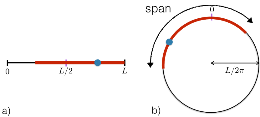
Figure 1: (Color online) a) Brownian motion with reflecting boundary conditions (RBC) at $x=0$ and $x=L$. The thick (red) region indicates the space already covered by the walker up to time $t$, starting at $x_{0}=L/2$. The circle denotes the current position, at time $t$, of the walker. b) The same walker on a ring, i.e., with periodic boundary conditions (PBC), starting at $0$. The thick (red) region, indicating the covered space up to time $t$, is equivalent to the span ${\cal S}(t)$ (the spatial extent of the visited region) of a walker on the infinite line. In both cases, the cover time $t_{c}$ is the first time at which the entire domain becomes red.

In this Letter, we present exact results for the full distribution of $t_{c}$ in $d=1$ for a RW in the Brownian limit (i.e., the long time scaling limit of a discrete-time RW on a lattice), on a finite interval of size $L$ for both reflecting (RBC) and periodic (PBC) boundary conditions (see Fig. 1). In the case of PBC, the RW takes place on a ring of size $L$ and evidently the distribution of $t_{c}$ is independent of the starting point, while it depends explicitly on the starting point $x_{0}\in[0,L]$ in the case of RBC. In the latter case, for simplicity, we present the results only when the walker starts at the center of the interval, i.e., at $x_{0}=L/2$. We show that, in the Brownian limit (with a diffusion constant $D$), the probability density function (PDF) of $t_{c}$ is given by

$$\mathrm{Prob.}[t_{c}=t|L]=\frac{4D}{L^{2}}\,f_{1}^{\mathrm{R|P}}\left(\frac{4D\,t}{L^{2}}\right),$$ (1)

where $\mathrm{R|P}$ denotes respectively the RBC and the PBC. The exact scaling functions $f_{1}^{\rm R}(x)$ and $f_{1}^{\rm P}(x)$ are given respectively in Eqs. (10) and (14), along with their asymptotics in Eqs. (11) and (15). Plots of these two scaling functions are shown in Fig. 2.

Another interesting question concerns the statistics of the cover time $t_{c}$ where there are $N$ independent walkers. This problem of multiple independent random walkers naturally arises in various search problems where there is a team of $N$ independent searchers, as opposed to a single searcher. Various observables associated with this multiple random walker process have been studied over the last few decades, such as the first passage time to the origin Redner2001 ; our_review ; oshanin ; debacco , the number of distinct and common sites visited by these walkers larralde:1992 ; Yuste ; Tamm ; Kundu:2013bk ; Turban , the statistics of the maximum displacement convex_hull_PRL ; convex_hull_JSP ; Paul ; Anupam , the statistics of records records , etc. For $N$ walkers, the cover time $t_{c}$ is the minimum time needed for all sites to be visited at least once by at least one of the walkers. In the literature, only the mean cover time was computed and that too only for $N=2$ with PBC in $1d$ Hemmer:1998es . It is evident that the average cover time will decrease with increasing $N$, but how does it decrease for large $N$? In this Letter, we generalize our result for the cover time distribution for one walker to arbitrary $N$ walkers in $1d$, both for RBC and PBC (for a plot of these distributions for different $N$, see Fig. 3). In particular, we show that the mean cover time, for both boundary conditions, decreases for large $N$ as

$$\frac{4D\,\langle t_{c}\rangle}{L^{2}}\approx\frac{1}{4\ln N}\;.$$ (2)

However, it turns out that the fluctuations around the mean are sensitive to the boundary conditions. Indeed we show that for large $N$, the random variable $t_{c}$ approaches to

$$\frac{4D\,t_{c}}{L^{2}}\approx\frac{1}{4\ln N}-\frac{1}{4(\ln N)^{2}}\,\chi_{\rm R,P}\;,$$ (3)

where $\chi_{\rm R}$ and $\chi_{\rm P}$ are two $N$-independent distinct random variables with non-trivial PDFs given respectively by (with $x\in(-\infty,+\infty)$)

$${\rm Prob.}[\chi_{\rm R}=x]=g_{\rm R}(x)=2\,e^{-x-e^{-x}}\left(1-e^{-e^{-x}}\right)$$ (4)

plotted in Fig. 4, and

$${\rm Prob.}[\chi_{\rm P}=x]=g_{\rm P}(x)=4\,e^{-2x}\,K_{0}(2\,e^{-x})$$ (5)

where $K_{0}$ is the modified Bessel function. The function $g_{\rm P}(x)$ is plotted in Fig. 4.

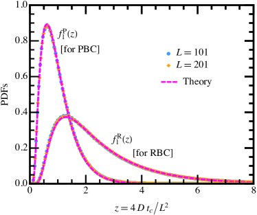
Figure 2: (Color online). The PDFs of the scaled cover time for a single lattice RW with RBC and PBC for sizes $L=101$ (blue) and $L=201$ (orange). The collapsed scaling data are compared to theoretical scaling functions (dashed lines) in the Brownian limit in Eq. (1) with $D=1/2$, where $f_{1}^{\rm R|P}(z)$ are given respectively in Eqs. (10) and (14).

Single walker (reflecting case).— Let us start by first considering the case of a single Brownian motion on the interval $[0,L]$ starting at $x_{0}$, with RBC at $x=0$ and $x=L$. The cover time $t_{c}$ in this case is clearly the first time when the walker has hit both boundaries at $x=0$ and $x=L$. It is useful to consider the cumulative distribution ${\rm Prob.}[t_{c}>t|x_{0}]$. If $t_{c}>t$, this means that at time $t$ one of the boundaries has not been hit up to time $t$. This means that ${\rm Prob.}[t_{c}>t|x_{0}]={\rm Prob.}[L\;{\rm\;is\;unhit\;up\;to\;time\;}t]+{\rm Prob.}[0\;{\rm is\;unhit\;up\;to\;time\;}t]-{\rm Prob.}[{\rm both\;are\;unhit\;up\;to\;time\;}t]$. All the three probabilities can be computed by solving the standard backward Fokker-Planck equation for the survival probability $S(x_{0},t)$ ($x_{0}$ being the starting position of the walker)

$$\frac{\partial S(x_{0},t)}{\partial t}=D\frac{\partial^{2}S(x_{0},t)}{\partial x_{0}^{2}}\;$$ (6)

with appropriate boundary conditions at $x_{0}=0$ and $x_{0}=L$. For example, ${\rm Prob.}[L\;{\rm\;is\;unhit\;up\;to\;time\;}t]=S_{\rm AR}(x_{0},t)$ where the subscript ${\rm A}$ indicates an absorbing boundary condition at $x_{0}=L$ (i.e., $S(x_{0}=L,t)=0$), while the subscript ${\rm R}$ refers to the reflecting boundary condition at $x_{0}=0$, (i.e., $\partial_{x_{0}}S(x_{0},t)|_{x_{0}=0}=0$) Redner2001 ; satya_review ; our_review . Hence we have

$${\rm Prob.}[t_{c}>t|x_{0}]=S_{\rm AR}(x_{0},t)+S_{\rm RA}(x_{0},t)-S_{\rm AA}(x_{0},t)\;,$$ (7)

where the subscripts refer to the boundary conditions. These survival probabilities can be computed exactly from Eq. (27) using standard methods Redner2001 ; our_review ; chupeau_convex , for instance either by expanding into Fourier modes (satisfying the appropriate boundary conditions) or equivalently by taking a Laplace transform with respect to time $t$ (for details, see SM ). For convenience, we will choose $x_{0}=L/2$, for which by symmetry $S_{\rm AR}(x_{0}=L/2,t)=S_{\rm RA}(x_{0}=L/2,t)$. For this choice, one can show that $S_{\text{AA}}(L/2,t)=S_{1}(4Dt/L^{2})$ and $S_{\text{AR}}(L/2,t)=S_{\text{RA}}(L/2,t)=S_{2}(4Dt/L^{2})$, where

$$S_{1}(z)=\frac{4}{\pi}\sum_{n=0}^{\infty}\frac{(-1)^{n}}{(2n+1)}\,e^{-(2n+1)^{2}\pi^{2}z/4}\;,$$ (8)

and

$$S_{2}(z)~{}=\frac{4}{\pi}\sum_{n=0}^{\infty}\frac{(-1)^{n}\cos[(2n+1)\pi/4]}{(2n+1)}\,e^{-(2n+1)^{2}\pi^{2}z/16}\;.$$ (9)

Hence we have $\mathrm{Prob.}[t_{c}>t|L]=F_{1}(4Dt/L^{2})$, where the scaling function $F_{1}(z)=2S_{2}(z)-S_{1}(z)$. Taking derivative with respect to $z$ yields the PDF in Eq. (1) with the scaling function $f^{\rm R}_{1}(z)$ given explicitly by

$$f_{1}^{\rm R}(z)=S^{\prime}_{1}(z)-2\,S^{\prime}_{2}(z)\;,$$ (10)

where $S_{1}(z)$ and $S_{2}(z)$ are given in Eqs. (8) and (9). The tails of the scaling function are given explicitly by (see Supp. Mat. SM )

$$f_{1}^{\mathrm{R}}(z)\sim\begin{cases}(6/\sqrt{\pi})z^{-3/2}e^{-9/(4z)}&\text{as}~{}z\to 0,\\ \pi/\bigl{(}2\sqrt{2}\bigr{)}\,e^{-\pi^{2}z/16}&\text{as}~{}z\to\infty.\end{cases}$$ (11)

A plot of this scaling function is shown in Fig. 2, where it is also compared to the simulation results. Simulations were done for a RW on a lattice of $L=101$ and $L=201$ sites with reflecting boundary conditions, which in the long time limit collapses to the Brownian scaling function in Eqs. (1) and (10).

Single walker (periodic case).— We now consider the cover time for a single RW on a ring of length $L$. In this case, the distribution of $t_{c}$ is independent of $x_{0}$, which we take it to be at $0$ (see Fig. 1 b)). We first show that the cumulative probability ${\rm Prob.}[t_{c}>t|L]$ on the ring can be mapped exactly onto the cumulative distribution of the span ${\cal S}(t)$ of the walker at time $t$ on an infinite line – the span being the length of the covered region by the walker up to time $t$. The probability that $t_{c}>t$ indicates that at time $t$ the ring has not been covered by the walker (see Fig. 1 b)). Since the ring has not been fully traversed at time $t$, the walker does not realize that it is on a ring. Thus one can think of the walk taking place on an infinite line and ${\rm Prob.}[t_{c}>t|L]$ on the ring is just the probability that the span ${\cal S}(t)$ of the walker on the infinite line is less than $L$, i.e., one has the exact relation (see Fig. 1 b))

$${\rm Prob.}[t_{c}>t|L]={\rm Prob.}[{\cal S}(t)<L]\;.$$ (12)

The PDF of the span ${\cal S}(t)$ on the infinite line is known hughes_book , ${\rm Prob.}[{\cal S}(t)=s]=(1/\sqrt{4Dt})h_{1}(s/\sqrt{4Dt})$ where

$$h_{1}(y)=\frac{8}{\sqrt{\pi}}\sum_{m=1}^{\infty}(-1)^{m+1}m^{2}e^{-m^{2}\,y^{2}}\;.$$ (13)

Therefore, taking derivative of Eq. (12) with respect to $t$, we obtain the PDF of the cover time on a ring as in Eq. (1) where the scaling function $f_{1}^{\rm P}(z)=1/(2\,z^{3/2})h_{1}(1/\sqrt{z})$. Using the explicit expression of $h_{1}(y)$ in Eq. (13) we then get

$$f_{1}^{\rm P}(z)=\frac{4}{\sqrt{\pi}z^{3/2}}\sum_{m=1}^{\infty}(-1)^{m+1}m^{2}e^{-m^{2}/z}\;.$$ (14)

The tails of this function are given by (see Supp. Mat. SM )

$$f_{1}^{\mathrm{P}}(z)\sim\begin{cases}\bigl{(}4/\sqrt{\pi}\bigr{)}z^{-3/2}e^{-1/z}&\text{as}~{}z\to 0,\\ \pi^{2}z\,e^{-\pi^{2}z/4}&\text{as}~{}z\to\infty.\end{cases}$$ (15)

For a plot of this scaling function, see Fig. 2.

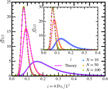
Figure 3: (Color online). Main: The PDFs of the scaled cover time (16) for different $N$ with RBC. For each $N$, the numerical results were obtained for lattice RW of size $L=201$ as in Fig. 2. The (magenta) dashed lines are the exact theoretical scaling functions in the Brownian limit with $D=1/2$, and are given by $f_{N}^{\rm R}(z)$ in Eq. (17). Inset: Same data as shown in the main panel but for PBC. The (magenta) dashed lines correspond to the exact theoretical results given by $f_{N}^{\rm P}(z)$ in (24).

Multiple walkers (reflecting case). — Here we consider, for simplicity, $N$ independent walkers all starting at the same point $x_{0}$. Using the mutual independence of the $N$ walkers, the cumulative cover time distribution for $N$ walkers is clearly given by ${\rm Prob.}[t_{c}>t|x_{0},N]=[S_{\text{AR}}(x_{0},t)]^{N}+[S_{\text{RA}}(x_{0},t)]^{N}-[S_{\text{AA}}(x_{0},t)]^{N}$. Choosing as before $x_{0}=L/2$, we find that

$$\mathrm{Prob.}[t_{c}=t|x_{0}=L/2,N]=\frac{4D}{L^{2}}\,f_{N}^{\mathrm{R}}\left(\frac{4Dt}{L^{2}}\right),$$ (16)

with the superscript $\mathrm{R}$ denoting RBC and the scaling function given by

$$f_{N}^{\mathrm{R}}(z)=-F_{N}^{\prime}(z)\;,\;{\rm where}\;\;F_{N}(z)=2\bigl{[}S_{2}(z)\bigr{]}^{N}-\bigl{[}S_{1}(z)\bigr{]}^{N}\;,$$ (17)

where $S_{1,2}(z)$ are given in Eqs. (8) and (9). A plot of this function for different values of $N$ is shown in the main panel of Fig. 3 where it is compared to simulations, with an excellent agreement. For $N\geq 2$, the asymptotics of $f_{N}^{\mathrm{R}}(z)$ are given by

$$f_{N}^{\mathrm{R}}(z)\sim\begin{cases}2N(N-1)/(\pi z)\,e^{-1/(2z)}&\text{as}~{}z\to 0,\\ (N\pi^{2}/8)(2\sqrt{2}/\pi)^{N}\,e^{-N\pi^{2}z/16}&\text{as}~{}z\to\infty\;.\end{cases}$$ (18)

Note that the small $z$ asymptotics of $f_{N}^{\rm R}(z)$ are quite different for $N=1$ (11) and $N\geq 2$ (18).

One naturally wonders whether there exists a limiting distribution of $t_{c}$ for large $N$. We first estimate the mean cover time $4D\langle t_{c}\rangle/L^{2}=\int_{0}^{\infty}F_{N}(z)\,dz$, where $F_{N}(z)$ is the cumulative scaling function given in Eq. (17). For large $N$, one expects that $\langle t_{c}\rangle$ is small. Hence, the integral $\int_{0}^{\infty}F_{N}(z)\,dz$ is dominated by the small $z$ behavior of $F_{N}(z)$. For small $z$, one can show from Eqs. (8) and (9) using Poisson summation formula (see SM for details), that $S_{1}(z)\sim 1-4\sqrt{z/\pi}\,e^{-1/(4z)}$ and $S_{2}(z)\sim 1-2\sqrt{z/\pi}\,e^{-1/(4z)}$. Substituting this behavior in Eq. (17) and exponentiating for large $N$ we get

$$F_{N}(z)\approx 2\,e^{-u_{N}(z)}-e^{-2\,u_{N}(z)}\;,\;u_{N}(z)=\frac{2\sqrt{z}}{\sqrt{\pi}}N\,e^{-1/(4z)}\;.\;$$ (19)

Therefore $F_{N}(z)\sim 1$ as long as $u_{N}(z)\ll 1$ (which happens for $z<1/(4\ln N)$), while $F_{N}(z)$ is exponentially small in $N$ for $z>1/(4\ln N)$. Hence, to leading order for large $N$, $4D\langle t_{c}\rangle/L^{2}=\int_{0}^{\infty}F_{N}(z)\,dz\approx 1/(4\ln N)$, as announced in Eq. (2). In addition, we can also compute the limiting distribution from Eq. (19) by expanding around $z=1/(4\ln N)$. We set $z=1/(4\ln N)-x/(4(\ln N)^{2})$, where we assume that the scaled fluctuation $x$ is of order ${\cal O}(1)$. Substituting this $z$ in $u_{N}(z)$ in Eq. (19) and expanding for large $N$, one gets to leading order $u_{N}(z)\approx e^{-x}$. Hence, in this limit, one obtains $F_{N}(z)\to 2\,e^{-e^{-x}}-e^{-2\,e^{-x}}$. Taking derivative with respect to $x$ gives the limiting PDF of $t_{c}$ as announced in Eq. (4).

Multiple walkers (periodic case) — We now consider $N$ independent walkers on a ring of size $L$, all starting at the same point $0$. As in the $N=1$ case discussed earlier, the cumulative cover time distribution is exactly related to the cumulative distribution of the span ${\cal S}_{N}(t)$ of $N$ walkers on an infinite line, all starting at the same point, via the relation

$${\rm Prob.}[t_{c}>t|L,N]={\rm Prob.}[{\cal S}_{N}(t)<L]\;.$$ (20)

The study of the PDF of ${\cal S}_{N}(t)$ was initiated in Ref. larralde:1992 and was recently computed exactly for all $N$ in Kundu:2013bk . It was shown in Ref. Kundu:2013bk that ${\rm Prob.}[{\cal S}_{N}(t)=s]=(1/\sqrt{4Dt})h_{N}(s/\sqrt{4Dt})$ where the $N$-dependent scaling function $h_{N}(y)$ is given by

$$h_{N}(y)=\int_{0}^{\infty}dl_{1}\int_{0}^{\infty}dl_{2}~{}\delta(y-l_{1}-l_{2})\frac{\partial^{2}g^{N}}{\partial l_{1}\partial l_{2}}\;.$$ (21)

Here $g(l_{1},l_{2})$ is the scaled cumulative joint distribution of the maximum and the minimum of a single BM, starting at the origin on an infinite line and is given by Kundu:2013bk :

$$g(l_{1},l_{2})=\frac{4}{\pi}\sum_{n=0}^{\infty}\frac{1}{2n+1}~{}\text{{sin}}\left[\frac{(2\,n+1)\pi l_{2}}{{l_{1}}+l_{2}}\right]e^{-\left[\frac{(2n+1)\pi}{2(l_{1}+l_{2})}\right]^{2}}.$$ (22)

As in the case of $N=1$, taking derivative of Eq. (20) with respect to $t$, we get

$$\mathrm{Prob.}[t_{c}=t|L,N]=\frac{4D}{L^{2}}\,f_{N}^{\mathrm{P}}\left(\frac{4Dt}{L^{2}}\right),$$ (23)

with the superscript ${\rm P}$ denoting PBC. The scaling function $f_{N}^{\rm P}(z)$ is given by

$$f_{N}^{\rm P}(z)=\frac{1}{2\,z^{3/2}}\,h_{N}\left(\frac{1}{\sqrt{z}}\right)\;,$$ (24)

where $h_{N}(y)$ is given in Eq. (21). In the inset of Fig. 3, we show a plot of $f_{N}^{\rm P}(z)$ for different $N$ and compare it to numerical results. The asymptotic tails of $f_{N}^{\rm P}(z)$ for $N\geq 2$ are given by

$$f_{N}^{\mathrm{P}}(z)\sim\begin{cases}\sqrt{2}N(N-1)/(\sqrt{\pi}z^{3/2})\,e^{-1/(2z)}&\text{as}~{}z\to 0,\\ (a_{N}\,z/2)\,e^{-N\pi^{2}z/4}&\text{as}~{}z\to\infty\;,\end{cases}$$ (25)

where $a_{N}$ can be computed explicitly (see SM ). As in the reflecting case (18), the behavior for $z\to 0$ is quite different for $N=1$ and $N\geq 2$.

We now turn to the limiting distribution of $t_{c}$ for large $N$ for PBC. In the context of the span distribution, the limiting form of the scaling function $h_{N}(y)$ was already analyzed for large $N$ in Ref. Kundu:2013bk and it was found that

$$h_{N}(y)\approx 2\,\sqrt{\ln N}\,{\cal D}\left(2\,\sqrt{\ln N}\,(y-2\,\sqrt{\ln N})\right)\;,$$ (26)

where the function ${\cal D}(s)=2\,e^{-s}\,K_{0}(2e^{-s/2})$ was obtained as a convolution of two Gumbel laws. Substituting this result (26) in Eq. (24) one finds that this function $f_{N}^{\rm P}(z)$ has a sharp peak at $z=1/(4\ln N)$. To analyze the large $N$ scaling limit of $f_{N}^{\rm P}(z)$, we set $z=1/(4\ln N)-x/(4(\ln N)^{2})$ as in the reflecting case. Expanding for large $N$, we get $f_{N}^{\rm P}(z)\approx 8(\ln N)^{2}{\cal D}(2\,x)$. Using $dz=dx/(4(\ln N)^{2})$, one immediately obtains the results for the periodic case announced in Eqs. (3) and (5).

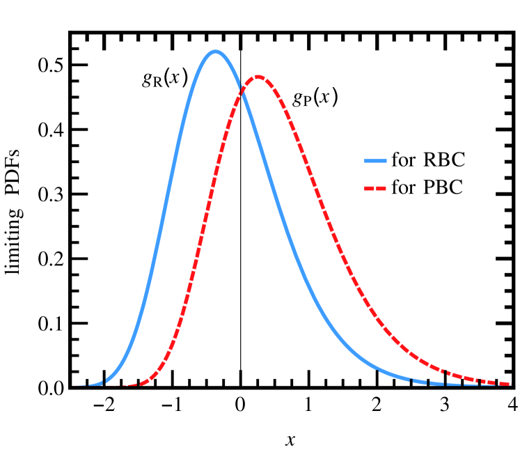
Figure 4: Plot of the limiting PDFs of $t_{c}$ (for $N$ RWs in the limit of large $N$) $g_{\rm R}(x)$ (for RBC) and $g_{\rm P}(x)$ (for PBC) given respectively in Eqs. (4) and (5).

Conclusion.— We have obtained the full PDF of the cover time $t_{c}$ for $N$ independent Brownian motions in one dimension, both for reflecting and periodic boundary conditions. Previously, only the first moment of $t_{c}$ was known in $1d$ for $N=1$ and $N=2$. Our results provide the first instance of exact cover time distributions for recurrent random walks, demonstrating clearly that this is different from a Gumbel law found recently for transient (i.e., non-recurrent) walks Chupeau:2015gp ; Belius . In addition, we have shown that in the limit of large $N$, the random variable $t_{c}$ approaches its average value $\langle t_{c}\rangle\approx L^{2}/(16\,D\,\ln N)$, with fluctuations decaying as $1/(\ln N)^{2}$. The centered and scaled distributions converge to two distinct and nontrivial $N$-independent scaling functions $g_{\rm R}(x)$ and $g_{\rm P}(x)$ given respectively in Eqs. (4) and (5) and plotted in Fig. 4. Another instance of recurrent RW is in $d=2$ for which the average value of $t_{c}$ has been well studied Aldous83 ; Broder_Karlin ; hilhorst ; dembo ; ding . However, determining its full PDF in $d=2$ for one or multiple ($N\geq 2$) walkers remains an outstanding challenge.

We thank the Indo-French Centre for the Promotion of Advanced Research under Project Number 5604-E.

Supplementary Material

We give some details about the results presented in the Letter not shown, for clarity, in the main text.

Reflecting boundary conditions (RBC). We compute the survival probability $S(x_{0},t)$ up to time $t$ of a $1d$ Brownian motion in $[0,L]$ starting at the initial position $x_{0}\in[0,L]$. It satisfies the backward Fokker-Planck equation our_review_app ; Redner2001_app

$$\frac{\partial S(x_{0},t)}{\partial t}=D\frac{\partial^{2}S(x_{0},t)}{\partial x_{0}^{2}},$$ (27)

where $D$ is the diffusion constant. This equation holds for $x_{0}\in[0,L]$, with the initial condition $S(x_{0},0)=1$ for $0<x_{0}<L$. We consider three different boundary conditions, as needed in the text. For example we denote by $S_{\rm AR}(x_{0},t)$ the survival probability corresponding to boundary conditions: absorbing (at $x_{0}=0$) and reflecting (at $x_{0}=L$). Similarly, we will also compute $S_{\rm RA}(x_{0},t)$ and $S_{\rm AA}(x_{0},t)$. By taking Laplace transform $\tilde{S}(x_{0},\lambda)=\int_{0}^{\infty}e^{-\lambda t}S(x_{0},t)\,dt$ in Eq. (27), and using the initial condition $S(x_{0},0)=1$, yields an ordinary differential equation

$$D\frac{d^{2}\tilde{S}(x_{0},\lambda)}{dx_{0}^{2}}-\lambda\tilde{S}(x_{0},\lambda)=-1\;.$$ (28)

This differential equation can be trivially solved with the appropriate boundary conditions at $x_{0}=0$ and $x_{0}=L$. For simplicity, we choose $x_{0}=L/2$. In this case we obtain

$$S_{\text{AA}}(L/2,t)=S_{1}\left(\frac{4Dt}{L^{2}}\right),$$ (29)

$$S_{\text{AR}}(L/2,t)=S_{\text{RA}}(L/2,t)=S_{2}\left(\frac{4Dt}{L^{2}}\right),$$ (30)

where

$$\int_{0}^{\infty}S_{1}(z)e^{-\lambda z}\,dz =\frac{1}{\lambda}\left[1-\frac{1}{\cosh\sqrt{\lambda}}\right],$$ (31)

$$\int_{0}^{\infty}S_{2}(z)e^{-\lambda z}\,dz =\frac{1}{\lambda}\left[1-\frac{\cosh\sqrt{\lambda}}{\cosh 2\sqrt{\lambda}}\right].$$ (32)

These Laplace transforms can be inverted by using the standard Bromwich contour in the complex $\lambda$-plane and calculating the residues at the poles. This gives the results announced in Eqs. (8) and (9) in the text:

$$S_{1}(z)=\frac{4}{\pi}\sum_{n=0}^{\infty}\frac{(-1)^{n}}{(2n+1)}\,e^{-(2n+1)^{2}\pi^{2}z/4}\;,$$ (33)

and

$$S_{2}(z)~{}=\frac{4}{\pi}\sum_{n=0}^{\infty}\frac{(-1)^{n}\cos[(2n+1)\pi/4]}{(2n+1)}\,e^{-(2n+1)^{2}\pi^{2}z/16}\;\;.$$ (34)

These series representations are very useful for calculating the large $z$ asymptotics, where only the $n=0$ term gives the leading contribution. For example, from Eq. (10) in the text and the $n=0$ terms in $S_{1}(z)$ and $S_{2}(z)$ in Eqs. (33) and (34), it gives the large $z$ asymptotics of $f_{1}^{\rm R}(z)$ in Eq. (11) in the text. Similarly, for $N$ walkers, the large $z$ asymptotics of the scaling function $f_{N}^{\rm R}(z)$ defined in Eq. (17) of the text can be derived from the leading $n=0$ term and this gives the second line of Eq. (18) of the text.

However, for small $z$, it is harder to compute the tail from the series representations in (33) and (34). In that case, one can use an alternative representation that can be obtained via the Poisson summation formula Poisson . Equivalently, we can derive it by inserting the following identity

$$\frac{1}{\cosh(p\sqrt{\lambda})}=2\sum_{n=0}^{\infty}(-1)^{n}e^{-(2n+1)p\sqrt{\lambda}},$$ (35)

in Eqs. (31) and (32) and then inverting the Laplace transform term by term. This gives, after straightforward algebra

$$S_{1}(z) =1-2\sum_{n=0}^{\infty}(-1)^{n}\mathrm{erfc}\left(\frac{2n+1}{2\sqrt{z}}\right),$$ (36)

$$S_{2}(z) =1-\sum_{n=0}^{\infty}\left(\sin\frac{n\pi}{2}+\cos\frac{n\pi}{2}\right)\mathrm{erfc}\left(\frac{2n+1}{2\sqrt{z}}\right)\;,$$ (37)

where $\mathrm{erfc}{(x)}=({2}/{\sqrt{\pi}})\int_{x}^{\infty}e^{-u^{2}}\,du$. Note that $\mathrm{erfc}{(x)}\approx e^{-x^{2}}/(x\sqrt{\pi})$ as $x\to\infty$. Consequently, for small $z$, keeping only terms up to $n=1$ in the sums in Eqs. (36) and (37) (higher order terms only give subleading corrections), gives

$$S_{1}(z)\approx 1-\frac{4\sqrt{z}}{\sqrt{\pi}}\,e^{-\frac{1}{4z}}+\frac{4\sqrt{z}}{3\sqrt{\pi}}\,e^{-\frac{9}{4z}}\;,$$ (38)

$$S_{2}(z)\approx 1-\frac{2\sqrt{z}}{\sqrt{\pi}}\,e^{-\frac{1}{4z}}-\frac{2\sqrt{z}}{3\sqrt{\pi}}\,e^{-\frac{9}{4z}}\;.$$ (39)

Consequently, the scaling function for the cover time PDF, $f_{1}^{\rm R}(z)=S_{1}^{\prime}(z)-2S_{2}^{\prime}(z)$, has the asymptotics announced in Eq. (11) of the text. Note that, for small $z$, the leading term $\propto e^{-1/(4z)}$ actually cancels in $f_{1}^{\rm R}(z)=S_{1}^{\prime}(z)-2S_{2}^{\prime}(z)$. Similarly, for $N$ walkers ($N\geq 2$), using Eq. (17) for $f_{N}^{\rm R}(z)$ in the text and the above properties in (38) and (39) we get the small $z$ asymptotics in the first line of Eq. (18) in the text. Note that the leading small $z$ behavior of $f_{N}^{\rm R}(z)$ is rather different for $N=1$ and $N\geq 2$.

Periodic boundary conditions (PBC). We start with the scaling function $f_{1}^{\rm P}(z)$ given in Eq. (14) in the text:

$$f_{1}^{\rm P}(z)=\frac{4}{\sqrt{\pi}z^{3/2}}\sum_{m=1}^{\infty}(-1)^{m+1}m^{2}e^{-m^{2}/z}\;.$$ (40)

This formula is useful for the small $z$ asymptotics. Indeed, keeping the $m=1$ term in (40) gives the first line of Eq. (15) in the text. However, this representation is not very convenient to derive the large $z$ asymptotics. For this, we could use the following identity:

$$1+2\sum_{m=1}^{\infty}(-1)^{m}e^{-m^{2}x}=2\sqrt{\frac{\pi}{x}}\sum_{n=0}^{\infty}e^{-\frac{\pi^{2}}{x}(n+1/2)^{2}}\;,\;\;\;\;x>0\;,$$ (41)

which can be easily derived from the Poisson summation formula Poisson . Taking derivative with respect to $x$ on both sides and setting $x=1/z$ one obtains

$$f_{1}^{\rm P}(z)=\sum_{n=0}^{\infty}\left[(2n+1)^{2}\,\pi^{2}\,z-2\right]e^{-\pi^{2}\,(n+1/2)^{2}\,z}\;.$$ (42)

For large $z$, the $n=0$ term provides the most dominant contribution, which gives the second line of Eq. (15) in the text. Using similar series representations for the function $g(l_{1},l_{2})$ defined in Eq. (22) in the text, and using results from Ref. Kundu_app for the asymptotics of $h_{N}(y)$, one obtains the asymptotic results announced in Eq. (25) of the text with the coefficient

$$a_{N}=4\pi^{3/2}N(N-1)~{}\left(4/\pi\right)^{N-2}~{}\Gamma([N-1]/2)/\Gamma(N/2)\;.$$ (43)

In particular one can check that $a_{1}=2\pi^{2}$, in agreement with the second line of Eq. (15) in the text.

References

- (1) O. Bénichou, C. Loverdo, M. Moreau, and R. Voituriez, Rev. Mod. Phys. 83, 81 (2011).
- (2) G. M. Viswanathan, V. Afanasyev, S. V. Buldyrev, E. J. Murphy, P. A. Prince, and H. E. Stanley, Nature 381, 413 (1996).
- (3) G. M. Viswanathan, S. V. Buldyrev, S. Havlin, M. G. E. da Luz, E. P. Raposo, and H. E. Stanley, Nature 401, 911 (1999).
- (4) G. M. Viswanathan, M. G. E. da Luz, E. P. Raposo, and H.E. Stanley, The Physics of Foraging (Cambridge Univ. Press, Cambridge, 2011).
- (5) M. F. Shlesinger, J. Phys. A: Math. Theor. 42, 434001 (2009).
- (6) For various stochastic search problems, see the special issue: The Random Search Problem: Trends And Perspectives, Eds. M. G. E. D. Luz, A. Grosberg, E. P. Raposo, and G. M. Viswanathan, J. Phys. A: Math. and Theor. 42, 430301-434017 (2009).
- (7) O. G. Berg, R. B. Winter, and P. H. Von Hippel, Biochemistry-US 20, 6929 (1981).
- (8) L. Mirny, Nature Phys. 4, 93 (2008).
- (9) J. Gorman, and E. C. Greene, Nat. Struct. Mol. Biol. 15, 768 (2008).
- (10) J. Gorman, A. J. Plys, M. L. Visnapuu, E. Alani, and E. C. Greene, Nat. Struct. Mol. Biol. 17, 932 (2010).
- (11) M. Eisenbach, and L. C. Giojalas, Nat. Rev. Mol. Cell Biol. 7, 276 (2006).
- (12) B. Meerson, and S. Redner, Phys. Rev. Lett. 114, 198101 (2015).
- (13) M. Chupeau, O. Bénichou, and R. Voituriez, Nat. Phys. 11, 844 (2015).
- (14) A. Z. Broder, in Proceedings of the Thirtieth Annual IEEE Symposium on Foundations of Computer Science, (IEEE, New York, 1989), p. 442.
- (15) D. J. Aldous, SIAM J. Discrete Math. 3,450 (1990).
- (16) D. J. Aldous, Z. Wahrscheinlichkeit 62, 36 (1983).
- (17) A. Z. Broder, and A. R. Karlin, J. Theor. Proba. 2, 101 (1989).
- (18) C. O. Yokoi, A. Hernández-Machado, and L. Ramírez-Piscina, Phys. Lett. A 145, 82 (1990).
- (19) M. J. A. M. Brummelhuis, and H. J .Hilhorst, Physica A 176, 387 (1991).
- (20) P. C. Hemmer, and S. Hemmer, Physica A 251, 245 (1998).
- (21) A. Dembo, Y. Peres, J. Rosen, and O. Zeitouni, Ann. Math. 160, 433 (2004).
- (22) N. Zlatanov, L. Kocarev, Phys. Rev. E 80, 041102 (2009).
- (23) J. Ding, Electron. J. Probab. 17, 1 (2012).
- (24) D. Belius, Probab. Theory Related Fields 157, 635 (2013).
- (25) S. Redner, A Guide to First-Passage Processes (Cambridge University Press, Cambridge, England, 2001).
- (26) A. J. Bray, S. N. Majumdar, and G. Schehr, Adv. Phys. 62, 225 (2013).
- (27) C. Mejia-Monasterio, G. Oshanin, and G. Schehr, J. Stat. Mech. P06022 (2011).
- (28) U. Bhat, C. De Bacco, and S. Redner, J. Stat. Mech. P083401 (2016).
- (29) H. Larralde, P. Trunfio, S. Hamlin, H. E. Stanley, and G. H. Weiss, Nature (London) 355, 423 (1992).
- (30) L. Acedo, and S. B. Yuste, Recent Res. Devel. Stat. Phys. 2, 83 (2002).
- (31) S. N. Majumdar, and M. Tamm, Phys. Rev. E 86, 021135 (2012).
- (32) A. Kundu, S. N. Majumdar, and G. Schehr, Phys. Rev. Lett. 110, 220602 (2013).
- (33) L. Turban, J. Phys. A 47, 385004 (2014).
- (34) J. Randon-Furling, S. N. Majumdar, and A. Comtet, Phys. Rev. Lett. 103, 140602 (2009).
- (35) S. N. Majumdar, A. Comtet, and J. Randon-Furling, J. Stat. Phys, 138, 955 (2010).
- (36) P. L. Krapivsky, S. N. Majumdar, and A. Rosso, J. Phys. A: Math. Theor. 43, 315001 (2010).
- (37) A. Kundu, S. N. Majumdar, and G. Schehr, J. Stat. Phys. 157, 124 (2014).
- (38) G. Wergen, S. N. Majumdar, and G. Schehr, Phys. Rev. E 86, 011119 (2012).
- (39) B. D. Hughes, Random walks and random environments, Clarendon Press Oxford, (1995), see formula (6.331) p. 384.
- (40) See Supplemental Material for details.
- (41) S. N. Majumdar, Curr. Sci. 77, 370 (1999).
- (42) M. Chupeau, O. Bénichou, and S. N. Majumdar, Phys. Rev. E 91, 050104 (2015).

References

- (1) A. J. Bray, S. N. Majumdar, and G. Schehr, Adv. Phys. 62, 225 (2013).
- (2) S. Redner, A Guide to First-Passage Processes (Cambridge University Press, Cambridge, England, 2001).
- (3) See https://en.wikipedia.org/wiki/Poisson_summation_formula
- (4) A. Kundu, S. N. Majumdar, and G. Schehr, Phys. Rev. Lett. 110, 220602 (2013).