Cosmic ray heating in cool core clusters – II. Self-regulation cycle and non-thermal emission

Abstract

Self-regulated feedback by active galactic nuclei (AGNs) appears to be critical in balancing radiative cooling of the low-entropy gas at the centres of galaxy clusters and in regulating star formation in central galaxies. In a companion paper, we found steady-state solutions of the hydrodynamic equations that are coupled to the cosmic ray (CR) energy equation for a large cluster sample. In those solutions, radiative cooling in the central region is balanced by streaming CRs through the generation and dissipation of resonantly generated Alfvén waves and by thermal conduction at large radii. Here, we demonstrate that the predicted non-thermal emission resulting from hadronic CR interactions in the intra cluster medium exceeds observational radio (and gamma-ray) data in a subsample of clusters that host radio mini halos (RMHs). In contrast, the predicted non-thermal emission is well below observational data in cooling galaxy clusters without RMHs. These are characterized by exceptionally large AGN radio fluxes, indicating high CR yields and associated CR heating rates. We suggest a self-regulation cycle of AGN feedback in which non-RMH clusters are heated by streaming CRs homogeneously throughout the central cooling region. We predict radio micro halos surrounding the AGNs of these CR-heated clusters in which the primary emission may predominate the hadronically generated emission. Once the CR population has streamed sufficiently far and lost enough energy, the cooling rate increases, which explains the increased star formation rates in clusters hosting RMHs. Those could be powered hadronically by CRs that have previously heated the cluster core.

1 Introduction

The central cooling time of the intracluster medium (ICM) of approximately half of all galaxy clusters is less than 1 Gyr, establishing a population of cool core (CC) clusters (Cavagnolo et al., 2009; Hudson et al., 2010). Since this cooling time falls below the cluster formation time by up to an order of magnitude, a copious amount of cold gas is expected to precipitate from the hot gaseous atmospheres and to form stars at rates up to several hundred $\mathrm{M}_{\odot}~{}\mathrm{yr}^{-1}$ (see Peterson & Fabian, 2006, for a review). The absence of radiative cooling and star formation at the predicted high rates calls for a heating mechanism that stabilizes the system. A promising framework is provided by energy feedback from an active galactic nucleus (AGN) at the cluster centre that accretes cooling gas and launches relativistic jets, which inflate radio lobes that are co-localized with the cavities seen in the X-ray maps. As the energy is transferred to the surrounding gas, this offsets radiative cooling until the heating reservoir is exhausted and the cooling gas can fuel the central AGN again, thus establishing a tightly self-regulated feedback loop. However, there has been little direct evidence supporting the existence of this hypothetical feedback cycle. In this paper, we will provide empirical evidence for such a self-regulating heating/cooling cycle and present a theoretical model to explain the underlying physics.

Because the energetics of AGN feedback is more than sufficient to balance radiative cooling, it has been suggested that AGN feedback can transform CC into non-CC clusters (Guo & Oh, 2009; Guo & Mathews, 2010). However, correlating the cavity enthalpy with the central gas entropy demonstrates that CC clusters cannot be transformed into non-CC clusters on the buoyancy time-scale due to the weak coupling of the mechanical to internal energy of the cluster gas (Pfrommer et al., 2012). This calls for a process that operates on a slower time-scale than the sound crossing time. Several physical processes associated with the rising radio lobes have been proposed to be responsible for the heating, including mixing (Kim & Narayan, 2003; Yang & Reynolds, 2016b), redistribution of heat by buoyancy-induced turbulent convection (Chandran & Rasera, 2007; Sharma et al., 2009) and dissipation of mechanical heating by outflows, lobes or sound waves from the central AGN (e.g., Churazov et al., 2001; Brüggen & Kaiser, 2002; Ruszkowski & Begelman, 2002; Gaspari et al., 2012). Also the role of thermal conduction in combination with AGN feedback has been explored (Kannan et al., 2016; Yang & Reynolds, 2016a).

As those jet-inflated lobes rise in the cluster potential, they excite gravity modes (Reynolds et al., 2015), which successively decay and generate turbulence that dissipates and heats the cluster gas (e.g., Zhuravleva et al., 2014). Recent micro-calorimetric X-ray observations of the core of the Perseus cluster find a low ratio of the turbulent-to-thermal pressure of 4% (Hitomi Collaboration et al., 2016). Such low-velocity turbulence cannot propagate far from the excitation site without being replenished, requiring turbulence to be generated in situ throughout the core or to be transported (non-thermally) from the radio lobes.

There is an alternative that explains the slow dissipation rate (acting on the Alfvén crossing time) and operates homogeneously throughout the cluster core. Relativistic particles (called cosmic rays, CRs) that are accelerated in the relativistic jet are likely mixed into the ambient thermal plasma during the buoyant rise of radio lobes (Sijacki et al., 2008; Guo & Mathews, 2011; Pfrommer, 2013). As they propagate from the injection site, they are following the ubiquitous magnetic fields (Kuchar & Enßlin, 2011) that redistribute their momenta to homogeneously fill the central core before they propagate towards larger radii. Fast-streaming CRs along the magnetic field excite Alfvén waves through the “streaming instability” (Kulsrud & Pearce, 1969). Scattering on this wave field limits the macroscopic speed of GeV CRs to velocities of order the Alfvén speed. Non-linear Landau damping of these Alfvén waves provides a means of transferring CR energy to the cooling gas. This may provide an efficient mechanism of suppressing the cooling catastrophe of cooling cores (Loewenstein et al., 1991; Guo & Oh, 2008; Enßlin et al., 2011; Fujita & Ohira, 2011; Pfrommer, 2013; Wiener et al., 2013).

To scrutinize this model, we compiled a large sample of 39 CC clusters in our first companion paper (Jacob & Pfrommer, 2017, hereafter JP17) and found steady-state solutions that match all observed density and temperature profiles well. In those models radiative cooling is balanced by CR heating in the cluster centres and by thermal conduction on larger scales. Most importantly we found a continuous sequence of cooling properties in our sample: clusters hosting radio mini halos (RMHs) are characterized by the largest cooling radii, star formation and mass deposition rates and thus signal the presence of a higher cooling activity. Correspondingly, more CRs are needed to balance cooling in those clusters.

RMHs are radio-emitting diffuse sources with typical radial extensions of 100 to 200 kpc that are centred on some CC clusters (Giacintucci et al., 2014). The detection of unpolarized radio synchrotron emission from RMHs proves the existence of volume-filling magnetic fields and CR electrons in the cooling regions of those clusters. In contrast, Mpc-sized giant radio halos occur in a fraction of X-ray luminous non-CC clusters that are currently merging with another cluster (see e.g. Feretti et al., 2012, for a review).

In this second paper about CR heating in CC clusters, we assess the viability of our steady-state solutions by comparing the resulting non-thermal radio and gamma-ray emission to observational data (similarly to Pfrommer & Enßlin, 2004b; Colafrancesco & Marchegiani, 2008; Fujita & Ohira, 2012, 2013). As CR protons interact inelastically with the ambient gas protons, they produce primarily pions (provided their energy exceeds the kinematic threshold of the reaction). Neutral pions decay into gamma-rays and charged pions produce secondary positrons and electrons that emit radio-synchrotron radiation. Confronting our model predictions with data enables us to put forward an observationally supported model for self-regulated feedback heating, in which an individual cluster is either stably heated, predominantly cooling, or is transitioning from one state to the other.

Our paper is structured as follows. In Section 2, we briefly discuss the cluster sample and the density and CR pressure profiles that we base our analysis on. In Sections 3 and 4, we compare the non-thermal emission of our steady-state solutions to observational radio and gamma-ray data, respectively. In Section 5, we present the emerging picture of the self-regulation cycle of CC clusters and conclude in Section 6.

Throughout this paper, we use a standard cosmology with a present-day Hubble factor $H_{0}=70~{}\mathrm{km~{}s}^{-1}\mathrm{Mpc}^{-1}$, and density parameters of matter, $\Omega_{\mathrm{m}}=0.3$, and due to a cosmological constant, $\Omega_{\Lambda}=0.7$.

2 Cluster Properties

Our analysis is based on the cluster sample in JP17. Here, we briefly introduce and characterize this sample, describe fits to the density profiles and show the employed CR pressure profiles.

2.1 Sample selection

Our cluster sample consists of 39 CC clusters from the Archive of Chandra Cluster Entropy Profile Tables, ACCEPT (Cavagnolo et al., 2009) and has been detailed in JP17; here we only provide an overview of the selection criteria. The clusters are chosen such that they either show non-thermal emission or are promising targets for such an emission component. In particular, the sample includes the 15 clusters with a confirmed RMH in Giacintucci et al. (2014). Most of the remaining clusters are selected due to the high expected gamma-ray emission from pion decay (Pinzke et al., 2011). Since these predictions derive from observed density profiles and a universal, simulation-based CR model (Pinzke & Pfrommer, 2010), they also represent the X-ray brightest CCs for which Chandra data is available in the ACCEPT data base. Table 1 lists the clusters in our sample together with the observed quantities from the literature that are relevant for our analysis.

The redshift distribution of this sample is not homogeneous since clusters with RMHs have larger redshifts than most clusters without an RMH (shown in fig. 1 in JP17). This is likely due to a selection bias that results from an inherent surface brightness limit of a typical RMH observation, which favours more compact, massive clusters at intermediate redshifts. However, most clusters in our sample have similar masses (within a factor of four), independent of whether they host an RMH or not, and we have only a few outliers at the low- and high-mass ends. To highlight the unbiased sample, we analyse our core sample that is almost unbiased in mass and display the outliers for visual purposes in more transparent colours where appropriate.

We further characterize our sample in Fig. 1 by showing the bolometric X-ray luminosity of all ACCEPT clusters as a function of the X-ray temperature (an observational proxy for cluster mass). We highlight the CC clusters of our sample with RMHs (blue circles) and the clusters without RMHs (red diamonds). More transparent colours indicate our low- or high-mass clusters, respectively. The figure shows that the selected clusters span the whole parameter range that is covered by the ACCEPT sample. Still, clusters with an RMH have systematically higher bolometric luminosities than clusters without RMHs.

While our unbiased cluster sample (full colours) spans a narrow range in $M_{200}$ and $T_{\mathrm{X}}$ of a factor of three, the bolometric X-ray luminosity varies by over two orders of magnitudes, indicating the enormous variance in core densities. CC clusters (including our entire sample) populate the upper envelope of the $L_{\mathrm{bol}}$–$T_{\mathrm{X}}$ relation due to the higher than average density of these systems at fixed cluster mass.

Table 1: Cluster sample.

Cluster	$z$(1)	$M_{200}^{\mathrm{(2)}}$	$kT_{\mathrm{X}}^{\mathrm{(1)}}$	SFR${}_{\mathrm{IR}}^{\mathrm{(3)}}$	$r_{\mathrm{cool}}^{\mathrm{(4)}}$	$F_{\nu,\mathrm{NVSS}}^{\mathrm{(5)}}$	$F_{\nu,\mathrm{mod}}$	$F_{\gamma,\mathrm{obs}}^{\mathrm{(6)}}$	$F_{\gamma,\mathrm{mod}}$	$F_{\gamma,>1\mathrm{~{}GeV}}$
		$\left(\times 10^{14}\right)$						$\left(\times 10^{-11}\right)$	$\left(\times 10^{-11}\right)$	$\left(\times 10^{-11}\right)$
		$\mathrm{~{}M_{\odot}}$	keV	$\mathrm{M_{\odot}\;yr^{-1}}$	kpc	mJy	mJy	$\mathrm{ph\,cm^{-2}\,s^{-1}\!\!\!}$	$\mathrm{ph\,cm^{-2}\,s^{-1}\!\!\!}$	$\mathrm{ph\,cm^{-2}\,s^{-1}}\!\!\!$
A 3112	0.0720	6.5a	4.28	4.2a	19.8	…000	9.16$\times$101	27.3a00	1.75	1.75
MKW3S	0.0450	5.1a	3.50	…	6.6	${}^{\mathrm{a\,}}$1.15$\times$105	8.79$\times$105	….00	…	0.50
Virgo (M87)	0.0044	1.4b	2.50	0.24b	9.5	${}^{\mathrm{a\,}}$1.39$\times$105	1.25$\times$101	135b.000	51.52	51.52
A 2052	0.0353	4.4a	2.98	1.4a	15.0	${}^{\mathrm{a\,}}$5.50$\times$103	8.43$\times$105	24c.000	2.88	0.80
Centaurus	0.0109	5.3a	3.96	0.18b	10.9	${}^{\mathrm{a\,}}$3.80$\times$103	7.11$\times$105	801d.000	25.30	5.12
Hydra A	0.0549	6.2a	4.30	3.77b	18.9	${}^{\mathrm{a\,}}$4.08$\times$104	1.00$\times$102	19.6a00	3.17	3.17
A 4059	0.0475	6.6a	4.69	0.57b	7.3	${}^{\mathrm{a\,}}$1.28$\times$103	3.99$\times$105	9.1a00	0.25	0.25
A 262	0.0164	1.9a	2.18	0.54a	5.8	${}^{\mathrm{a\,}}$6.57$\times$101	0.22$\times$105	9.3a00	0.13	0.13
A 3581	0.0218	1.8a	2.10	…	12.9	${}^{\mathrm{b\,}}$6.46$\times$102	2.27$\times$105	110c.000	1.69	0.47
A 2199	0.0300	6.4a	4.14	0.58b	13.1	${}^{\mathrm{a\,}}$3.58$\times$103	3.47$\times$101	19.8a00	4.74	4.74
A 1644	0.0471	10.0a	4.60	…	9.1	${}^{\mathrm{b\,}}$9.84$\times$101	1.07$\times$105	16a.000	0.10	0.10
MKW 4	0.0198	1.4a	2.16	0.03b	7.6	${}^{\mathrm{b\,}}$1.71$\times$101	0.36$\times$105	….00	…	0.13
A 539	0.0288	4.4a	3.24	…	2.5	${}^{\mathrm{b\,}}$6.30$\times$103	0.14$\times$105	….00	…	0.05
A 1795	0.0625	12.8a	7.80	…	20.0	${}^{\mathrm{a\,}}$9.25$\times$102	1.23$\times$102	5.8a00	3.33	3.33
A 2597	0.0854	5.7a	3.58	3.23b	34.1	${}^{\mathrm{a\,}}$1.88$\times$103	2.59$\times$102	4.400	3.33	3.33
A 133	0.0558	6.5a	3.71	…	18.7	${}^{\mathrm{a\,}}$1.67$\times$102	2.78$\times$101	7.6a00	0.96	0.96
A 496	0.0328	7.1a	3.89	…	17.0	${}^{\mathrm{b\,}}$1.21$\times$102	2.05$\times$101	25.2a00	1.45	1.45
A 907	0.1527	6.4c	5.04	…	8.5	${}^{\mathrm{b\,}}$6.86$\times$101	2.48$\times$101	….00	…	0.22
PKS 0745	0.1028	9.8a	8.50	17.2a	44.5	${}^{\mathrm{b\,}}$2.37$\times$103	1.37$\times$103	82c.000	45.26	12.65
AWM 7	0.0172	7.2a	3.71	…	5.4	${}^{\mathrm{b\,}}$2.90$\times$103	1.73$\times$105	384d.000	4.73	0.96
ZwCl 1742	0.0757	13.1a	4.40	2.02b	13.4	${}^{\mathrm{b\,}}$9.12$\times$101	5.82$\times$101	10.4a00	1.16	1.16
A 1991	0.0587	0.9c	5.40	…	17.8	${}^{\mathrm{b\,}}$3.90$\times$101	2.52$\times$101	….00	…	0.83
A 383	0.1871	5.0c	3.93	5.58b	32.5	${}^{\mathrm{c\,}}$4.09$\times$101	9.79$\times$101	….00	…	0.60
A 85	0.0558	10.9a	6.90	0.61b	20.0	${}^{\mathrm{b\,}}$5.67$\times$101	1.91$\times$102	18a.000	5.91	5.91
Perseus (A 426)	0.0179	8.6a	6.79	34.46b	34.2	${}^{\mathrm{a\,}}$2.28$\times$104	1.10$\times$102	0.014e	0.003	38.27
A 2029	0.0765	12.9a	7.38	…	24.5	${}^{\mathrm{b\,}}$5.28$\times$102	2.56$\times$102	328d.000	23.14	4.68
A 2390	0.2301	24.8d	9.16	40.6b	18.9	${}^{\mathrm{b\,}}$2.35$\times$102	2.37$\times$102	43c.000	4.73	1.32
A 478	0.0883	11.7a	7.07	2.39b	32.0	${}^{\mathrm{a\,}}$3.69$\times$101	2.15$\times$102	12.7a00	2.63	2.63
2A 0335+096	0.0347	4.5a	2.88	7c.00	31.4	${}^{\mathrm{a\,}}$3.67$\times$101	3.31$\times$102	6.7a00	15.53	15.53
A 2204	0.1524	8.3a	6.97	14.7a	41.1	${}^{\mathrm{c\,}}$6.93$\times$101	7.51$\times$102	13c.000	15.53	4.34
Ophiuchus	0.0280	40.5a	11.79	…	13.3	${}^{\mathrm{b\,}}$2.88$\times$101	3.51$\times$102	2622d.000	336.41	68.01
ZwCl 3146	0.2900	12.5c	12.80	65.51b	43.8	${}^{\mathrm{d\,}}$9.58$\times$101	1.21$\times$103	….00	…	3.85
MS 1455.0+2232	0.2590	4.8c	4.51	9.46b	44.6	${}^{\mathrm{d\,}}$1.93$\times$101	2.62$\times$102	….00	…	0.97
RX J1720.1+2638	0.1640	8.7c	5.55	…	32.5	${}^{\mathrm{d\,}}$8.77$\times$101	1.35$\times$103	….00	…	9.42
A 1835	0.2532	17.5d	7.65	235.37b	49.2	${}^{\mathrm{c\,}}$3.93$\times$101	1.12$\times$103	….00	…	5.02
RX J1532.9+3021	0.3450	7.9c	5.44	97a.00	51.1	${}^{\mathrm{c\,}}$2.28$\times$101	7.99$\times$102	….00	…	2.26
RX J1504.1-0248	0.2150	15.1c	8.90	140d.00	57.0	${}^{\mathrm{b\,}}$6.05$\times$101	2.19$\times$103	96c.000	33.70	9.42
RBS 0797	0.3540	9.7c	6.43	…	51.5	${}^{\mathrm{a\,}}$2.17$\times$101	9.21$\times$102	….00	…	2.26
RX J1347.5-1145	0.4510	26.1c	10.88	…	37.8	${}^{\mathrm{d\,}}$4.59$\times$101	3.00$\times$103	257d.000	24.90	5.03

• (1) Taken from the ACCEPT homepage (Cavagnolo et al., 2009)

• (2) a) Pinzke et al. (2011) b) Urban et al. (2011) c) $M_{500}$ from Laganá et al. (2013) d) $M_{500}$ from Ettori et al. (2010), for c) and d) we use $M_{200}=200\times 4\pi\rho_{\mathrm{crit}}r_{200}^{3}/3$

• (3) a) O’Dea et al. (2008) b) Hoffer et al. (2012) c) Donahue et al. (2007) d) Ogrean et al. (2010)

• (4) We define the cooling radius $r_{\mathrm{cool}}$ as the radius where the cooling time is $1\mathrm{~{}Gyr}$.

• (5) a) Bîrzan et al. (2004) b) sources from the NVSS Source catalogue browser with distance to ACCEPT coordinates $<15\mathrm{~{}arcsec}$, except for A 539 ($1.08\mathrm{~{}arcmin}$) and MKW 4 ($1.32\mathrm{~{}arcmin}$) c) Sayers et al. (2013) d) Coble et al. (2007)

• (6) a) Ackermann et al. (2014) ($>1\mathrm{~{}GeV}$) b) Abdo et al. (2009) ($>1\mathrm{~{}GeV}$) c) Dutson et al. (2013) ($>0.3\mathrm{~{}GeV}$) d) Ackermann et al. (2010) ($0.2-100\mathrm{~{}GeV}$) e) Aleksić et al. (2012) ($>1\mathrm{~{}TeV}$); these values are upper limits except for Virgo/M87 (Abdo et al., 2009)

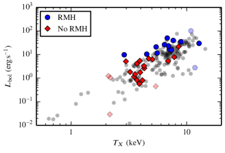
Figure 1: Bolometric X-ray luminosity and X-ray temperature (as an observational proxy for cluster mass) of all clusters in the ACCEPT data base (grey data points). Clusters of our sample are highlighted with blue circles if they host an RMH and with red diamonds if not. Remarkably, clusters with an RMH have typically higher bolometric luminosities than clusters without RMHs. Clusters at the low- and high-mass end (that do not belong to our core sample) are shown with transparent colours.

2.2 Density profiles

The non-thermal radio and gamma-ray emission depend on the density profiles of the clusters, either directly since the hadronic reaction is a two-body process with an emissivity that scales with the product of gas and CR density or indirectly through the magnetic field, which assumes a density dependence through the magnetic flux-freezing condition. Here, we use fits to observationally inferred density profiles. If we were to use the density profiles of our steady-state solutions as derived in JP17, this would only result in small changes and have no influences on our conclusions.

For 15 clusters, we use the fits by Vikhlinin et al. (2006) and Landry et al. (2013) who use the formula

$$n_{\mathrm{p}}n_{\mathrm{e}}=\frac{n_{0}^{2}\,\left(r/r_{\mathrm{c}}\right)^{-\alpha}}{\left[1+\left(r/r_{\mathrm{c}}\right)^{2}\right]^{3\beta-\alpha/2}}\frac{1}{\left[1+\left(r/r_{\mathrm{s}}\right)^{\gamma}\right]^{\varepsilon/\gamma}}+\frac{n_{\mathrm{02}}^{2}}{\left[1+\left(r/r_{\mathrm{c2}}\right)^{2}\right]^{3\beta_{2}}},$$ (1)

where $n_{\mathrm{e}}/n_{\mathrm{p}}=1.19$ (see also Appendix B.1).

We obtain the density profiles for the remaining clusters by performing our own fits. To this end, we use the data points provided on the ACCEPT homepage. Since the Chandra data only cover the centres of most clusters, we find that a single beta profile is sufficient to describe the data and adopt the following profile

$$n_{\mathrm{e}}=n_{0}\left[1+\left(r/r_{\mathrm{c}}\right)^{2}\right]^{-3\beta/2}$$ (2)

in a suitable radial range. The fit results together with the radial range of applicability can be found in Appendix A in Table 4.

2.3 CR pressure profiles

We use a CR population that is able to balance radiative cooling in the centres of CC clusters through the excitation of Alfvén waves. These waves get dissipated, which implies a volumetric heating rate (Wentzel, 1971)

$$\mathcal{H}_{\mathrm{cr}}=-\mn@boldsymbol{\upsilon}_{\mathrm{st}}\mn@boldsymbol{\cdot\nabla}P_{\mathrm{cr}}.$$ (3)

Here, $P_{\mathrm{cr}}$ is the CR pressure and the streaming velocity is given by

$$\mn@boldsymbol{\upsilon}_{\mathrm{st}}=-\mathrm{sgn}(\mn@boldsymbol{B\cdot\nabla}P_{\mathrm{cr}})\mn@boldsymbol{\upsilon}_{\mathrm{A}},$$ (4)

where $\mn@boldsymbol{B}$ is the magnetic field, $\mn@boldsymbol{\upsilon}_{\mathrm{A}}=\mn@boldsymbol{B}/\sqrt{4\uppi\rho}$ is the Alfvén velocity and $\rho$ is the mass density.

Such a CR population is described by the steady-state solutions from JP17, which are obtained by solving the hydrodynamic equations that are coupled to the CR energy equation. In those solutions, radiative cooling is balanced by thermal conduction at large scales and CR heating in the central regions, giving rise to a small mass deposition rate of cooling gas that precipitates out of the hot atmosphere at a level that is typically 10 per cent of the observed infrared (IR) star formation rate (SFR). The resulting CR pressure profiles approximately follow the thermal pressure profiles in the central region (i.e., $X_{\mathrm{cr}}\equiv P_{\mathrm{cr}}/P_{\mathrm{th}}\approx\mathrm{const.}$) and fall off rapidly outside the radius at which conductive heating starts to dominate. The model parameters are chosen such that the solutions are physical and that the radial extent over which CR heating dominates is maximized (for more detail please refer to JP17).

The steady-state solutions are only valid in a certain radial range, i.e., between the radii $r_{\mathrm{in}}$ and $r_{\mathrm{out}}$. To determine the non-thermal emission, we extend the solutions to the centre of the cluster with a constant value. Since the outer radius can vary substantially from cluster to cluster, we extrapolate the profile to $200\mathrm{~{}kpc}$ if $r_{\mathrm{out}}$ is smaller than that, which is the case for 25 out of 39 clusters. Beyond $200\mathrm{~{}kpc}$, the CR pressure has typically dropped significantly, such that the hadronically induced fluxes are fully determined by the emission at smaller radii and the exact cut-off radius becomes unimportant. For the extrapolation to larger radii, we use a power law. The final CR pressure profile is then given by

$$P_{\mathrm{cr,ex}}(r)=\begin{cases}P_{\mathrm{cr}}(r_{\mathrm{in}})&r<r_{\mathrm{in}}\\ P_{\mathrm{cr}}(r)&r_{\mathrm{in}}<r<r_{\mathrm{out}}\\ P_{\mathrm{cr}}(r_{\mathrm{out}})\left(\frac{r}{r_{\mathrm{out}}}\right)^{\alpha_{P_{\mathrm{cr}}}}&r>r_{\mathrm{out}}\end{cases}$$ (5)

with $\alpha_{P_{\mathrm{cr}}}=\left.\mathrm{d}\ln P_{\mathrm{cr}}/\mathrm{d}\ln r\right|_{r_{\mathrm{out}}}$.

3 Radio emission

Hadronic interactions between relativistic CRs and the ambient cluster medium lead to secondary electrons and hence synchrotron emission. Here, we compare the modelled radio emission of our steady-state CR population to observed data by the NRAO VLA Sky Survey (NVSS, Condon et al., 1998) as well as RMHs.

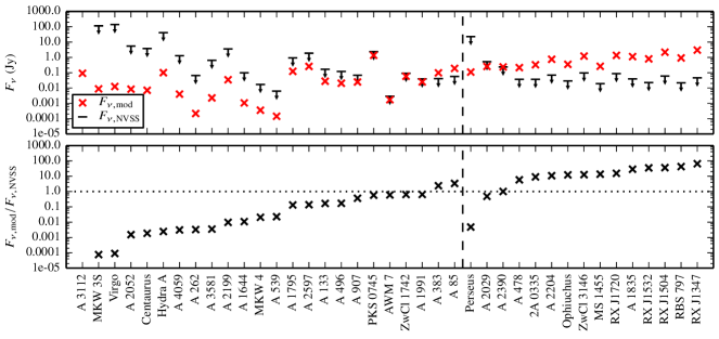
Figure 2: Comparison between the predicted secondary radio flux of our steady-state solutions and the 1.4 GHz flux measured by NVSS. Because the radio emission observed by NVSS likely acquires a partial contribution from primary accelerated CR electrons, it represents an upper limit to the hadronically generated secondary radio emission. The top panel shows the absolute flux values of a new predicted class of radio micro halos (left to the dashed line). In the bottom panel, we display the ratio of predicted to observed flux. For most clusters without RMHs the predicted flux is smaller than the flux observed by NVSS, whereas for RMH clusters the predicted flux is generally in conflict with the data. This excludes CR pressures at a level required to stably balance radiative cooling in most clusters hosting an RMH.

3.1 Emissivity

We calculate the radio emission closely following Pfrommer et al. (2008). For brevity, we only introduce the most important concepts here and provide the complete description in Appendix B.

The distribution of protons, which we describe in terms of the dimensionless proton momentum $p_{\mathrm{p}}=P_{\mathrm{p}}/(m_{\mathrm{p}}c)$, is given by

$$f_{\mathrm{p}}(p_{\mathrm{p}})=\frac{\mathrm{d}N}{\mathrm{d}p_{\mathrm{p}}\mathrm{d}V}=C_{\mathrm{p}}(r)p_{\mathrm{p}}^{-\alpha_{\mathrm{p}}}\theta(p_{\mathrm{p}}-q_{\mathrm{p}}).$$ (6)

It represents a power-law in momentum with spectral index $\alpha_{\mathrm{p}}=2.4$. Such a spectral index is expected for a CR population that was injected by an AGN and may have experienced a mild spectral steepening as a result of outwards streaming (Wiener et al., 2013). We enforce a lower momentum cut-off at $q_{\mathrm{p}}=0.5$ with the Heaviside step function $\theta(x)$. We denote the normalization by $C_{\mathrm{p}}(r)$ and specify it with the steady-state solutions for the CR pressure.

Hadronic CR proton interactions with the ICM produce secondary electrons. If radiative losses are taken into account, this population of secondary electrons reaches a steady state with a spectral index that is steepened by one, $\alpha_{\mathrm{e}}=\alpha_{\mathrm{p}}+1$ (Sarazin, 1999). The corresponding secondary synchrotron emissivity $j_{\nu}$ at frequency $\nu$ per steradian is given by

$$j_{\nu}=\frac{A_{\nu}}{4\pi}C_{\mathrm{p}}n_{\mathrm{N}}\frac{e_{B}}{e_{B}+e_{\mathrm{rad}}}\left(\frac{e_{B}}{e_{B_{\mathrm{c}}}}\right)^{(\alpha_{\nu}-1)/2}.$$ (7)

The emissivity depends on the normalization of the CR protons $C_{\mathrm{p}}$ and on the nucleon density $n_{\mathrm{N}}$, which is proportional to the electron number density introduced in Section 2.2. Moreover, it depends on the frequency-dependent normalization factor, $A_{\nu}$, the magnetic energy density, $e_{B}$, the energy density in radiation, $e_{\mathrm{rad}}$, a frequency dependent characteristic magnetic field strength, $e_{B_{\mathrm{c}}}$, and the radio spectral index $\alpha_{\nu}=(\alpha_{\mathrm{e}}-1)/2$.

Assuming an isotropic distribution of the CR electrons’ pitch angles, the synchrotron emissivity can be written in terms of the magnetic energy density $e_{B}=B^{2}/(8\pi)$. We parametrize the magnetic field strength as in JP17, which is motivated by analyses of deprojected Faraday rotation measure maps and minimum field estimates by radio observations with the LOw Frequency ARray (Vogt & Enßlin, 2005; Kuchar & Enßlin, 2011; de Gasperin et al., 2012),

$$B(r)=B_{0}\left(\frac{n_{\mathrm{e}}(r)}{0.01\mathrm{~{}cm^{-3}}}\right)^{\alpha_{B}}.$$ (8)

We adopt a magnetic field normalization $B_{0}=10\,\mathrm{\mu G}$ and a power law index of $\alpha_{B}=0.5$. This choice implies a radially constant Alfvén speed $\upsilon_{\mathrm{A}}$.

Additionally, the energy density from radiation fields attains contributions from the cosmic microwave background (CMB) and from stars and dust (SD) in the central galaxy, $e_{\mathrm{rad}}$. As a result, the synchrotron emissivity is modified because these emitting CR electrons suffer additional energy losses from inverse Compton scattering on the total radiation field. In the regime of weak fields ($e_{B}\ll e_{\mathrm{rad}}$), the emissivity strongly depends on the magnetic field strength (see equation 7). The radiation from stars and dust predominates within the central galaxy and exceeds the magnetic energy density up to a radius of $20$ – $40\mathrm{~{}kpc}$, depending on the particular cluster (see Fig. 10). At larger radii, the magnetic field starts to predominate as long as its energy density exceeds the energy density of the cosmic microwave background, $\varepsilon_{B}>\varepsilon_{\mathrm{CMB}}$, which is the case for $n_{\mathrm{e}}\gtrsim 10^{-3}\,\mathrm{cm}^{-3}$ or equivalently most of the cool core regions studied in this work ($r\lesssim 130--200$ kpc according to Fig. 10).

The emissivity scales with frequency as $j_{\nu}\propto\nu^{-\alpha_{\nu}}$. Here, $\alpha_{\nu}=(\alpha_{\mathrm{e}}-1)/2=1.2$, which is encapsulated in $e_{B_{\mathrm{c}}}$ and $A_{\nu}$. In the limit of large magnetic fields ($e_{B}\gg e_{\mathrm{rad}}$), the electrons loose all their energy to synchrotron radiation and not by inverse Compton scattering. Thus, to good approximation we can neglect the energy density in radiation in Equation (7). In this case, we obtain a weak scaling of the emissivity with magnetic field strength since then $j_{\nu}\propto\varepsilon_{B}^{(\alpha_{\nu}-1)/2}\approx\varepsilon_{B}^{0.1}$ for our choice of $\alpha_{\mathrm{e}}$. Because most of the secondary synchrotron emission is collected from radii between 20 and 100 kpc for which we are clearly in the magnetically dominated emission regime, the emissivity is mostly insensitive to the exact value of magnetic field strength and is thus directly proportional to the normalization of the CR distribution.

Using this emissivity, we can calculate theoretically expected surface brightness profiles, luminosities and fluxes for the available observations. In the main text, we focus on fluxes and surface brightness profiles, which we can directly compare to observations, and discuss the luminosities in Appendix C.

3.2 Comparison with NVSS data

We first compare the emission from the steady state CR population to the data from the NVSS. This survey detects point sources at 1.4 GHz with a restored beam of $45\mathrm{~{}arcsec}$ full width half-maximum (FWHM). These data include emission by primary electrons that are accelerated by the AGN combined with the secondary electrons injected in hadronic interactions between CRs and thermal protons. Therefore, the NVSS data have to be considered as upper limits for our purpose.

We track the radial extent of the CR population to a maximum radius of $r_{\mathrm{max},\parallel}=\max\left\{r_{\mathrm{out}},200\mathrm{~{}kpc}\right\}$. This choice ensures that we account for the entire CR energy in our non-thermal emission because in most clusters, the CR pressure drops steeply at radii well below $200\mathrm{~{}kpc}$ as a result of CR streaming. Moreover, this characteristic radius corresponds to a typical radial extent of an RMH. We verified that the radio flux does not depend on the precise choice of this radius because it is dominated by the central regions. However, $r_{\mathrm{max},\parallel}$ subtends an angle on the sky that is larger than the NVSS beam width for all clusters.

Hence for the flux calculations, we first project the emissivity along the radial direction and obtain the surface brightness as

$$S_{\nu}(r_{\bot})=2\int_{r_{\bot}}^{r_{\mathrm{max,\parallel}}}\mathrm{d}r\frac{rj_{\nu}(r)}{\sqrt{r^{2}-r_{\bot}^{2}}}.$$ (9)

To determine the fluxes as seen by NVSS, we cut out a cylinder with radius $r_{\mathrm{max},\bot}$ that corresponds to $22.5\mathrm{~{}arcsec}$, half of the FWHM of the beam, such that

$$F_{\nu}=2\pi\int_{0}^{r_{\mathrm{max},\bot}}\mathrm{d}r_{\bot}r_{\bot}S_{\nu}\left(r_{\bot}\right).$$ (10)

We present the resulting fluxes together with the observations in Fig. 2 and list them in Table 1.

In the upper panel of Fig. 2, we show the absolute values of the predicted flux at 1.4 GHz as well as the radio fluxes observed by NVSS. The bottom panel shows their ratio. We separate clusters with and without an RMH and order each group according to the flux ratio. The upper panel shows that the predicted fluxes span orders of magnitude ranging from $10^{-4}$ to $10\mathrm{~{}Jy}$. The synchrotron flux predictions for clusters without an RMH are significantly smaller than for clusters hosting an RMH, whereas the fluxes from NVSS are often larger for clusters without RMHs.

There is an even stronger correlation in the flux ratios. Due to our ordering of the clusters, the flux ratio increases from left to right. Interestingly, the flux ratios for clusters with an RMH are generally much larger than for clusters without an RMH. Moreover, there is a smooth transition from the clusters without to the clusters with an RMH. An exception is Perseus with a very small flux ratio. The reason for this is the exceptionally strong NVSS source Perseus A since the predicted flux is in line with that of the other clusters.

We find that most flux ratios in clusters without an RMH are smaller than unity but almost exclusively exceed unity in RMH clusters. Thus, the level of CR pressure required to stably heat the interiors is in conflict with radio observations for RMH clusters while the secondary radio emission resulting from hadronic CR interactions is well below the observed fluxes in clusters without RMHs. Together with the gradual transition between the two populations this may indicate a self-regulated feedback loop. On the one side, the cooling gas in non-RMH clusters may be stably balanced by CR heating, while RMH clusters appear to be out of balance and predominantly cooling. This interpretation is further discussed in Section 5.

Table 2: Properties of the radio mini halos.

Cluster	$r_{\mathrm{RMH}}^{\mathrm{(1)}}$	$F_{\mathrm{RMH,obs}}^{\mathrm{(1,2)}}$	$F_{\mathrm{RMH,mod}}^{\mathrm{(2)}}$
	kpc	mJy	mJy
Perseus (A 426)	130	3020	4914
A 2029	270	19.5	728
A 2390	250	28.3	348
A 478	160	16.6	411
2A 0335+096	70	21.1	1475
A 2204	50	8.6	688
Ophiuchus	250	83.4	8718
ZwCl 3146	90	5.2	1184
MS 1455.0+2232	120	8.5	288
RX J1720.1+2638	140	72.0	1989
A 1835	240	6.1	1449
RX J1532.9+3021	100	7.5	782
RX J1504.1-0248	140	20.0	2637
RBS 0797	120	5.2	946
RX J1347.5-1145	320	34.1	3221

• (1) Giacintucci et al. (2014) and references therein

• (2) All fluxes correspond to $\nu=1.4\mathrm{~{}GHz}$.

3.3 Radio mini halos

The sources detected by the NVSS are point sources and can only be upper limits for our predictions since they also include primary emission from the central galaxy and its AGN. The observed RMHs allow us to test the extended radio emission from a CR population that is able to balance cooling. To this end, we study the fluxes of all RMHs and compare the surface brightness profiles of individual clusters to the observations by Murgia et al. (2009). In the end, we discuss the robustness of our conclusions with respect to changes in the parametrization of the magnetic field.

3.3.1 RMH fluxes

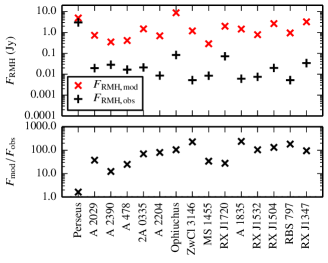
Figure 3: Comparison between the predicted fluxes for the RMHs and the observations from Giacintucci et al. (2014). All predicted secondary radio fluxes exceed the observations by a substantial margin (with the exception of Perseus that is only barely excluded). Thus, this excludes CR pressures at a level that is required to stably balance radiative cooling in the central cluster regions exhibiting an RMH.

Here, we compare our modelled secondary RMH fluxes to the observed values at $1.4\mathrm{~{}GHz}$ in Giacintucci et al. (2014). The hadronically induced RMH fluxes at this frequency from our CR population are determined as in Section 3.2. In contrast to the previous calculation, we now integrate the radio flux out to the radius $r_{\mathrm{max,\bot}}=\min\left\{r_{\mathrm{RMH}},r_{\mathrm{max,\parallel}}\right\}$. The radius $r_{\mathrm{RMH}}$ denotes the (average) radius of the RMH as determined by Giacintucci et al. (2014, see Table 2).

We show the results in Fig. 3. The upper panel displays the model predictions and observational fluxes, the lower panel their ratio. Clearly, the predicted flux exceeds the observed flux in all clusters by up to three orders of magnitude. This demonstrates that the secondary radio emission from a CR population that is able to balance radiative cooling is excluded by data. Conversely, this also means that if RMHs are powered by hadronic CR interactions, those CRs have insufficient pressure to heat the cluster gas.

While Perseus is formally excluded based on a moderate overproduction of the RMH flux by a factor of 1.6, uncertainties in the magnetic field model and the extent of the CR distribution along the line of sight could make it consistent with the observational RMH data.

3.3.2 Surface brightness profiles

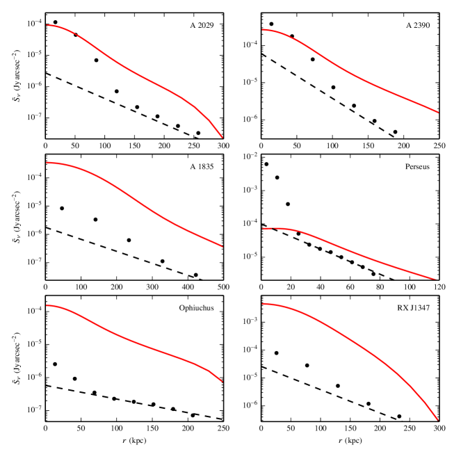
Figure 4: We compare the predicted radio surface brightness profiles of secondary synchrotron emission (red) to data from Murgia et al. (2009) (black data points). The black dashed lines show their fits to the emission from the RMH after modelling the central AGN emission. The expected emission exceeds the observed data by up to two orders of magnitudes, which indicates that CR heating is not viable in those clusters at all scales (with the exception of Perseus that is only marginally excluded).

Murgia et al. (2009) analyse the surface brightness profiles of a sample of clusters with radio halos and RMHs. Six of their clusters also coincide with members of our sample so that we can test our model profiles. The surface brightness is in principle given by Equation (9), but for better comparison we smooth our brightness profiles to the resolution of the Very Large Array observations at 1.4 GHz as described in Murgia et al. (2009). Therefore, we convolve the surface brightness with a Gaussian beam of standard deviation $\sigma=\mathrm{FWHM}_{\mathrm{beam}}/(2\sqrt{2\log(2)})$,

$$\tilde{S}_{\nu}(r) = \!\frac{1}{2\pi\sigma^{2}}\int\mathrm{d}^{2}x^{\prime}S_{\nu}(|\mn@boldsymbol{x^{\prime}}|)\exp\left(-\frac{(\mn@boldsymbol{x}-\mn@boldsymbol{x^{\prime}})^{2}}{2\sigma^{2}}\right)$$

$$= \!\frac{1}{\sigma^{2}}\int_{0}^{\infty}\mathrm{d}xxS_{\nu}(x)\exp\left(-\frac{x^{2}+r^{2}}{2\sigma^{2}}\right)I_{0}\left(\frac{rx}{\sigma^{2}}\right),$$

where $I_{0}(x)$ denotes a modified Bessel function of the first kind. For the convolution, we assume that the surface brightness profile has dropped to zero beyond $r_{\mathrm{max,\parallel}}$.

In Fig. 4, we compare the expected surface brightness profiles (red) to the radio data (black dots) of Murgia et al. (2009). These data contain the central radio source and the RMH. After modelling the central AGN, the RMH contribution is shown as black dashed lines, which take the form of exponential profiles (Murgia et al., 2009). The modelled secondary profiles exceed the observed RMH profiles by a factor of two in Perseus and up to two orders of magnitude in RX J1347. In three cases the profiles exceed even the emission from the central galaxy. This demonstrates that the emission from a CR population that is able to balance radiative cooling would overproduce the radio emission in the core region delineated by the RMH emission, at least in those six clusters.

Hence, our predictions generally surpass the limits set by radio observations in clusters hosting an RMH, irrespective of whether we use NVSS data, RMH fluxes or surface brightness profiles. Perseus and A2390 are only excluded by a factor of a few to several and represent thus transitional objects. These systems can be made consistent with the observational radio data by either lowering $X_{\mathrm{cr}}$ and increasing $B_{0}$ by the same factor or by truncating the CR distribution along the line of sight, which would lower the predicted radio flux without affecting the central heating rate. With the exception of those clusters, CR heating plays no central role in balancing radiative cooling in RMH-hosting clusters. Before we turn our attention to the gamma-ray emission, we assess the robustness of our conclusions when varying the magnetic field model.

3.3.3 Modifying the magnetic field

Aside from the CR population, the CR heating rate and the radio emissivity depend on the magnetic field strength. In our model, we fix the normalization at $B_{0}=10\mathrm{~{}\mu G}$ at $n_{\mathrm{e}}=10^{-2}\,\mathrm{cm}^{-3}$ (see Section 3.1). Here, we investigate whether it is possible to find a combination of magnetic field and CR pressure that reproduces the RMH fluxes and still balances radiative cooling.

In the limit of strong magnetic fields ($\varepsilon_{B}\gg\varepsilon_{\mathrm{CMB}}$), the emissivity is proportional to $j_{\nu}\propto C_{\mathrm{p}}B^{\alpha_{\nu}-1}$. For our choices of the spectral index, $\alpha_{\nu}=1.2$ (see Appendix B.1), which means that the dependence of $j_{\nu}$ on the magnetic field is extremely weak. Hence, the emissivity and therefore surface brightness profiles and fluxes depend almost entirely on the CR population. In order to meet the fluxes from the RMH, we would need to reduce the number of CRs by at least a factor of 10 for most clusters (barring Perseus). If the shape of the CR profile remains the same, the CR heating rate is proportional to $\mathcal{H}_{\mathrm{cr}}\propto BC_{\mathrm{p}}$. To achieve the same amount of CR heating with the reduced CR population, we would thus have to increase the magnetic field by a factor of 10. However, magnetic fields of $B_{0}\approx 100\mathrm{~{}\mu G}$ or higher would imply a plasma $\beta$ factor (i.e., the ratio of thermal-to-magnetic pressure) of 0.1 instead of the observed values that are of order or larger than 20 in cool core regions. Such a strong magnetic field is excluded by Faraday rotation measurements and minimum energy arguments (Vogt & Enßlin, 2005; Kuchar & Enßlin, 2011; de Gasperin et al., 2012) and would be impossible to grow and maintain with a (turbulent) magnetic dynamo in the presence of a small turbulent-to-thermal energy density ratio of 4 per cent (Hitomi Collaboration et al., 2016).

For that reason, it is not possible to simultaneously reproduce the RMH fluxes and heat the cluster gas with CRs in the entire cool core region. One resort would be to refrain from maximal CR models that heat the entire radio emitting region of RMHs. Instead, we could concentrate on CR heating models for the central region that would dramatically reduce the required amount of CR energy and by extension also the level of secondary radio emission to get into agreement with RMH data. However, as we will discuss in Section 5, we present an alternative scenario that argues for a heating/cooling imbalance in RMH clusters, which show strong signs of cooling and star formation and for a stable balance in clusters without an observable RMH.

4 Gamma-ray emission

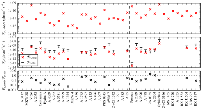
Figure 5: Comparison between the predicted gamma-ray flux as a result of hadronically induced pion decay and the constraints from observations. The top panel shows the predicted flux above $1\;\mathrm{GeV}$ for all clusters. In the middle panel we compare our predictions to the upper limits from Ackermann et al. (2014), Ackermann et al. (2010), Aleksić et al. (2012, Perseus) and Dutson et al. (2013) and the gamma-ray detection in the Virgo cluster (Abdo et al., 2009). We always compute the gamma-ray flux in the data-equivalent energy band (see Table 1 for details). The bottom panel illustrates the ratio between the predicted flux and the upper limits, indicating that present-day gamma-ray observations are not sensitive enough to seriously challenge the CR heating model (with the exceptions of 2A 0335 and A 2204, in which the CR heating model can be excluded based on gamma-ray observations).

Hadronic interactions between CRs and thermal protons produce neutral pions that decay into gamma-ray photons with a distinctive spectral signature in the differential source function that peaks at energies of half the pions’ rest mass. We use upper limits to the extended gamma-ray emission of galaxy clusters from Fermi and MAGIC to probe our model.

4.1 Pion decay luminosity

We follow Pfrommer et al. (2008) to determine the gamma-ray fluxes. Here, $s_{\gamma}(E_{\gamma})$ denotes the gamma-ray source function as a function of energy. The omnidirectional integrated gamma-ray source density between two energies $E_{1}$ and $E_{2}$ in units of photons per energy, per unit time, and per unit volume is then given by

$$\lambda_{\gamma}=\int_{E_{1}}^{E_{2}}\mathrm{d}E_{\gamma}s_{\gamma}(E_{\gamma}).$$ (12)

A detailed description of this formalism and the source function can be found in Appendix B.2. Integrating $\lambda_{\gamma}$ over the cluster volume yields the photon luminosity per unit time

$$\mathcal{L}_{\gamma}=\int\mathrm{d}V\lambda_{\gamma}=4\pi\int_{0}^{r_{\mathrm{max,\gamma}}}\lambda_{\gamma}r^{2}\mathrm{d}r,$$ (13)

where we use $r_{\mathrm{max,\gamma}}=\max\left\{r_{\mathrm{out}},200\mathrm{~{}kpc}\right\}$ as the upper integration limit. While the gamma-ray luminosity scales with cluster mass, there is an enormous range in non-thermal luminosity at fixed mass due to the large variance in gas density across our sample (see Fig. 11). The latter effect dominates the variance of the gamma-ray luminosity in our core sample as we quantitatively discuss in Appendix C. We obtain the gamma-ray fluence from the luminosity via

$$\mathcal{F}_{\gamma}=\frac{\mathcal{L}_{\gamma}}{4\pi D_{\mathrm{lum}}^{2}}$$ (14)

with the luminosity distance $D_{\mathrm{lum}}$.

4.2 Comparison with gamma-ray limits

We show the gamma-ray fluence above $1\mathrm{~{}GeV}$ for all clusters in the upper panel of Fig. 5 (see Table 1 for numerical values). The values are spread over three orders of magnitude between $10^{-12}$ and $10^{-9}\mathrm{~{}ph\,cm^{-2}\,s^{-1}}$. The fluences of clusters with an RMH are somewhat higher that for cluster without an RMH, with median values of $4\times 10^{-11}$ and $1\times 10^{-11}\mathrm{~{}ph\,cm^{-2}\,s^{-1}}$, respectively. This difference is smaller than the difference in gamma-ray luminosity of the two subsamples, because RMH clusters are on average at higher redshifts that partially compensates the larger luminosity (see Fig. 11).

Additionally, we compare our model fluences to observations. To this end, we employ the upper limits from Ackermann et al. (2010) who analyse data from the Fermi satellite for individual clusters. We also consider stacked Fermi limits provided by Ackermann et al. (2014) and Dutson et al. (2013), and we use Fermi observations of the Virgo cluster (Abdo et al., 2009) as well as MAGIC observations of the Perseus cluster (Aleksić et al., 2012). Note that all values are upper limits except for the Virgo cluster/M87.

Since these authors report their upper limits for different energy bands, we have to choose a data-equivalent energy band from $E_{1}$ to $E_{2}$ in Equation (12). In the middle panel of Fig. 5 we compare those observational gamma-ray limits to our predictions and show the ratio of predicted-to-expected gamma-ray emission in the bottom panel (upper limits and data-equivalent energy ranges are shown in Table 1). While the expectations for most clusters are below the upper limits, there are two clusters (2A 0335 and A 2204) that exceed the observational constraints. In those clusters, we can exclude the CR heating model based on gamma-ray observations alone. However, both of these clusters host an RMH for which our model is already excluded by the radio data. Hence, we conclude that while gamma-ray predictions come close to observational limits, present-day gamma-ray observations are not sensitive enough to seriously challenge the CR heating model.

Notable are the results for the Virgo cluster. Pfrommer (2013) constructs a CR population that simultaneously matches the observed gamma-ray emission and is able to stably balance radiative cooling while adopting a constant CR-to-thermal pressure ratio $X_{\mathrm{cr}}$ throughout the observed radio micro-halo (i.e., for $r<35$ kpc). Our steady-state model has also been constructed to offset radiative cooling but falls short of the observed gamma-ray emission by a factor of $2.6$. This is mainly because conductive heating starts to balance radiative cooling in our steady-state solution at radii $r\gtrsim 20$ kpc and causes the $X_{\mathrm{cr}}$ profile to steeply drop at this radius. Hence, the resulting hadronic gamma-ray emission falls short of the value it would have if conductive heating were absent. Moreover, in this work, we employ a slightly higher magnetic field, which translates to a slightly lower CR pressure for the identical heating rate, and a different cooling profile (which we infer from the ACCEPT data base).

The second cluster that has been studied in detail is the Perseus cluster. Here, we compare our model to TeV gamma-ray observations. At these energies the flux from the central galaxy NGC 1275 has dropped significantly so that gamma-rays from decaying pions should become dominant (Aleksić et al., 2012). The chosen energy range also explains the small absolute values for the gamma-ray fluence in Perseus. Although our model agrees with the current limits, we note that possible spectral steepening associated with CR streaming (Wiener et al., 2013) could weaken the MAGIC gamma-ray limit that assumes a single power-law spectrum to TeV energies (Ahnen et al., 2016).

5 Emerging picture

5.1 A self-regulated scenario for CR heating, cooling, and star formation

What is the conclusion of this at first sight disparate result that CR heating is excluded as the predominant source of heating in clusters that manifestly show non-thermal emission in form of RMHs? Let us summarize the main findings:

1. Our steady-state solutions of JP17 demonstrate that radiative cooling can be balanced by CR heating in the central region and by thermal conduction in the outer region. The resulting CR-to-thermal pressure in the central region attains values of $X_{\mathrm{cr}}\approx 0.05-0.1$ for clusters without an RMH, and shows systematically higher values of $X_{\mathrm{cr}}\approx 0.1-0.25$ for clusters with RMHs.

2. The level of hadronic radio and gamma-ray fluxes of our steady-state solutions is higher in clusters hosting an RMH because of the higher target density in RMH clusters (see Fig. 6) and excluded by observed NVSS and RMH fluxes.

3. In contrast, the predicted non-thermal emission is below observational radio and gamma-ray data in cooling galaxy clusters without RMHs (with the exception of A 383 and A 85).

4. Most importantly, the ratio of predicted-to-observed NVSS flux is dramatically increased in RMH clusters, the median of the flux ratio for both populations differs by a factor of a few hundred. In addition to the increased secondary flux noted in point (ii), the radio emission of the central AGN in clusters without a detected RMH is on average also much stronger. Because the AGN radio emission is a proxy for CR injection, this implies a significantly increased CR yield in the centre of those clusters. In particular, the predicted-to-observed NVSS flux ratio shows a continuous sequence from $10^{-4}$ at the lower end of non-RMH clusters to 100 for the upper end of RMH clusters (bottom panel in Fig. 2).

These different findings can be put together in form of a self-regulation scenario of AGN feedback in CC clusters for which we will provide further evidence below. A strong AGN radio emission signals the abundant injection of CRs into the centre. As these CRs stream outwards they can balance radiative cooling via Alfvén wave heating in the central regions while conductive heating takes over at larger radii. Here, the streaming CRs can heat the ICM homogeneously and locally stable (Pfrommer, 2013) by generating resonantly Alfvén waves so that mass deposition rates drop below $1~{}\mathrm{M}_{\odot}~{}\mathrm{yr}^{-1}$ (JP17).

Observationally, these CR heated systems could be associated with CC clusters that do not have an observable radio mini halo. Instead, we predict a new class of radio micro halos, that is associated with the radio synchrotron emission of primary and secondary CR electrons surrounding the central AGN. Radio micro halos have thus far escaped detection due to the small extent of the micro halo up to a few tens of kpcs and the large dynamic flux range of the jet and halo emission. An exception that supports this hypothesis is the only known micro halo in M87, the centre of the Virgo cluster, which can only be observed due to its close proximity of 17 Mpc. The expected hadronic gamma-ray emission can be identified with the low state of M87 (Pfrommer, 2013, see also Fig. 5).

Once the CR population has streamed sufficiently far from the centre and lost enough energy in exciting Alfvén waves, the gas cooling rate increases to values above $1~{}\mathrm{M}_{\odot}~{}\mathrm{yr}^{-1}$ that should also fuel star formation. Hence, this picture would predict enhanced levels of star formation in clusters in which CR heating ceases to be efficient, namely in those that are hosting an RMH. Our self-regulation scenario of CR-induced heating not only predicts stably heated clusters on the one side and cooling systems with abundant star formation on the other side, but also systems transitioning from one state to the other, such as the Perseus cluster, A 85, or A 383.

5.2 Supporting evidence for this picture

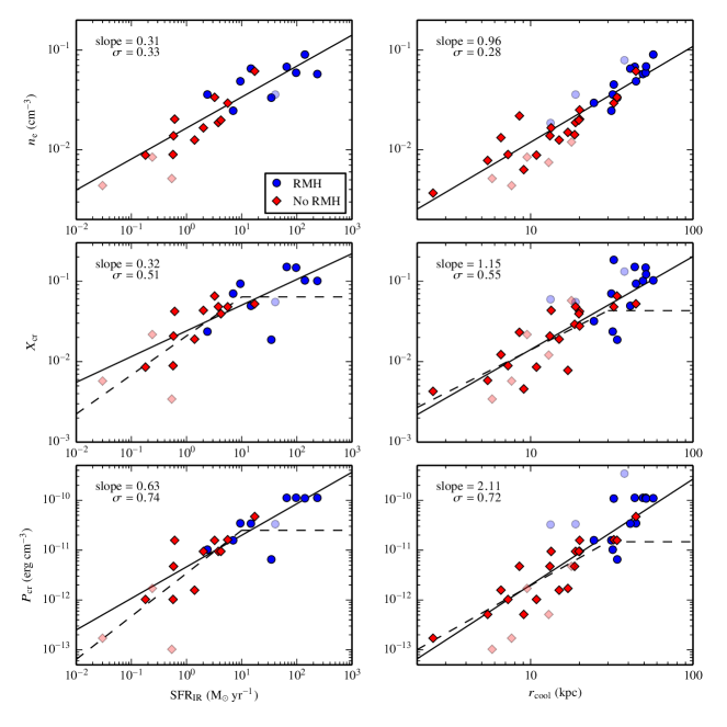
Figure 6: Relations between density (top), ratio of CR-to-thermal pressure (middle) and CR pressure (bottom) at a reference radius of $30\mathrm{~{}kpc}$ with the observed IR SFRs (left) and the cooling radius (right). The black lines are best-fitting power-law relations to our cluster core sample (full coloured data points). The more transparent data points denote clusters at the low- and high-mass end of our sample and are only shown for visual purposes. The slope and the vertical log-normal scatter $\sigma$ of the fit are indicated in the upper left of each panel. RMH clusters populate the upper end of these correlations, which is characterized by large SFRs and cooling radii. The top two panels represent purely observational correlations while the middle and bottom panels employ the CR and thermal pressure profiles of the steady-state solutions of JP17. Since for some clusters those solutions are excluded by radio data (see text), the dashed lines show fits to the remaining data points.

Table 3: Fit results for the correlations of the unbiased sample shown in Fig. 6 using a power-law relation of the form $y(x)=ax^{b}$, where $y(x)$ is specified in the first column.⁽¹⁾

	$a$	$b$	$\sigma$
$n_{\mathrm{e}}$(SFR)	$(1.6\pm 0.2)\times 10^{-2\hphantom{0}}$	$0.31\pm 0.04$	$0.33$
$kT$(SFR)	$(3.6\pm 0.2)\hphantom{\;\times\,10^{-13}}$	$0.06\pm 0.02$	$0.18$
$X_{\mathrm{cr}}$(SFR)	$(2.4\pm 0.4)\times 10^{-2\hphantom{0}}$	$0.32\pm 0.06$	$0.51$
$X_{\mathrm{cr}}$(SFR)val	$(2.1\pm 0.3)\times 10^{-2\hphantom{0}}$	$\hphantom{0}0.5\pm 0.1\hphantom{0}$	$0.37$
$P_{\mathrm{cr}}$(SFR)	$\hphantom{.0}(5\pm 1)\hphantom{.0}\times 10^{-12}$	$0.63\pm 0.09$	$0.74$
$P_{\mathrm{cr}}$(SFR)val	$(3.4\pm 0.8)\times 10^{-12}$	$\hphantom{0}0.9\pm 0.2\hphantom{0}$	$0.57$
$n_{\mathrm{e}}$ ($r_{\mathrm{cool}}$)	$(1.3\pm 0.3)\times 10^{-3\hphantom{0}}$	$0.96\pm 0.07$	$0.28$
$kT$ ($r_{\mathrm{cool}}$)	$(2.5\pm 0.4)\hphantom{\;\times\,10^{-4\hphantom{0}}}$	$0.15\pm 0.05$	$0.19$
$X_{\mathrm{cr}}$($r_{\mathrm{cool}}$)	$(1.0\pm 0.4)\times 10^{-3\hphantom{0}}$	$\hphantom{0}1.2\pm 0.1\hphantom{0}$	$0.55$
$X_{\mathrm{cr}}$($r_{\mathrm{cool}}$)val	$(1.3\pm 0.7)\times 10^{-3\hphantom{0}}$	$\hphantom{0}1.0\pm 0.2\hphantom{0}$	$0.52$
$P_{\mathrm{cr}}$($r_{\mathrm{cool}}$)	$(1.5\pm 0.8)\times 10^{-14}$	$\hphantom{0}2.1\pm 0.2\hphantom{0}$	$0.72$
$P_{\mathrm{cr}}$($r_{\mathrm{cool}}$)val	$\hphantom{0}(3\pm 2)\hphantom{.0}\times 10^{-14}$	$\hphantom{0}1.8\pm 0.3\hphantom{0}$	$0.68$

(1) These fits were performed in logarithmic space, the scatter $\sigma$ was obtained assuming a normal distribution for the deviation of the logarithm of the data to the mean relation. SFRs are given in $\mathrm{M_{\odot}\;yr^{-1}}$ and cooling radii in kpc. Densities are measured in $\mathrm{cm^{-3}}$, temperatures in keV and CR pressures in $\mathrm{erg\;cm^{-3}}$. The subscript “val” indicates the relations of the subsample of clusters for which our model is valid (dashed lines in Fig. 6).

To test this hypothesis, we scrutinize the cluster profiles for signs of such a cycle. To this end, we study observed quantities such as densities and SFRs as well as quantities that are predicted by the steady-state solutions such as the required CR pressures to balance radiative cooling.

First, we correlate the observed electron number density at a reference radius of $30\mathrm{~{}kpc}$ to the observed SFRs (top left panel of Fig. 6) and the cooling radius (top right panel). We find clear correlations of the form $n_{\mathrm{e}}\propto\mathrm{SFR}^{0.31}$ and $n_{\mathrm{e}}\propto r_{\mathrm{cool}}^{0.96}$. The log-normal scatter of these relations is $\sigma=0.33$ and $0.28$, respectively (see Table 3, for the fit parameters of the relation). Note that we exclude clusters at the low- and high-mass end of our sample (shown with transparent colours) for the fit. Most importantly, clusters hosting an RMH populate the upper end of the correlation that is characterized by the largest SFRs and cooling radii, i.e., RMHs signal cluster cores with enhanced cooling activity.

In order to connect these empirical findings to our theoretically motivated steady state solutions, we also determine the ratio of CR-to-thermal pressure inferred from our steady state solutions (JP17) at a reference radius of $30\mathrm{~{}kpc}$ and correlate it to the observed SFRs and the cooling radius (middle panels of Fig. 6). We see a correlation that has a similar dependence on SFR and $r_{\mathrm{cool}}$, albeit with a larger scatter. Dashed lines indicate the relations if only clusters are considered in which our model is valid, i.e., if we exclude clusters that host an RMH as well as A 383 and A 85. With the smaller sample, the relation is somewhat steeper for the SFRs but remarkably similar for the cooling radius. Clusters with an RMH require higher values of $X_{\mathrm{cr}}$ than clusters without RMHs to balance the enhanced cooling rates.

Last, we relate the CR pressure from the steady-state solutions at a reference radius of $30\mathrm{~{}kpc}$ to the observed SFR and cooling radius (bottom panels of Fig. 6). Since $P_{\mathrm{cr}}\propto X_{\mathrm{cr}}n_{\mathrm{e}}kT$ and the correlation of $kT$ with SFR and cooling radius shows no clear trends (see Table 3), we expect that the dependence of the CR pressure on SFR and cooling radius derive from the previous relations. Indeed, we obtain such steeper relations with a slope that is approximately given by the sum of the slopes for the density and $X_{\mathrm{cr}}$ relations. We find values of $0.63$ and $2.11$ for the scaling of $P_{\mathrm{cr}}$ with SFR and cooling radius, respectively. However, the correlations of the CR pressures show the largest scatter. As expected, clusters with an RMH have higher values for the CR pressure than clusters without RMHs. Dashed lines indicate again the results for the sample in which our steady-state solutions are in agreement with the observational radio (and gamma-ray) data.

In order to interpret these relations, we show in Fig. 7 the fit to the density profiles of five representative clusters along the correlations shown in Fig. 6, with a wide distribution in SFRs (RX J1504.1, ZwCl 3146, A 3112, Centaurus, MKW 4, moving from high to low SFRs). Note that the cluster with the lowest SFR is not part of our core sample due to its low virial mass. For each cluster the squares indicate the density at the reference radius of $30\mathrm{~{}kpc}$ and the circle marks the cooling radius $r_{\mathrm{cool}}$. Clearly, higher densities imply larger cooling rates and thus larger cooling radii. This puts a higher demand on the heating rate to balance the much increased cooling rate. Because these higher densities correlate with an increased SFR, the balance is apparently unsuccessful. This implies that these clusters are currently not stably heated but can cool to some extent. Hence, it might not be necessary for potential heating mechanisms to (fully) counteract radiative cooling in those clusters.

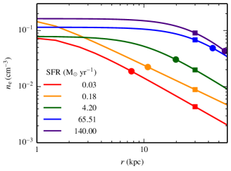
Figure 7: Representative electron number density profiles of five clusters with different SFRs, which are distributed along the correlation shown in Fig. 6. Note that the cluster with the lowest SFR is at the low-mass end and not part of our cluster core sample. The squares indicate the density at a reference radius of $30\mathrm{~{}kpc}$ whereas the circles denote the density at the cooling radius, $r_{\rm cool}$, of these systems.

As we demonstrate, CR heating is a prime candidate for providing the necessary heating rate: clusters with low SFRs can be CR heated unlike clusters with high SFRs. This is emphasized in Fig. 8 where we compare the ratio of modelled radio flux-to-NVSS flux with the SFR (left) and with the cooling radius (right). The figure shows that the flux ratio increases with SFR and cooling radius. Since the ratio of predicted-to-observed radio flux is a measure for the applicability of our model, this demonstrates that CR heating is viable in clusters with low SFRs and not applicable in clusters with higher SFRs. These results support the picture of a CR heating–radiative cooling cycle.

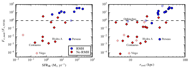
Figure 8: A measurement of the applicability of our model is the ratio of the modelled-to-observed NVSS flux. The modelled 1.4 GHz radio flux derives from the hadronically generated synchrotron emission of our steady-state CR population that stably balances radiative cooling. Here, we compare the flux ratio to the observed SFRs (left) and cooling radii (right) and separate clusters with and without an RMH by colour. Clusters with higher SFRs can not be successfully heated by streaming CRs while this is a likely possibility for clusters with lower SFRs, as expected for a self-regulated heating-cooling cycle.

A note on time-scales is in order since our picture requires that the density profile of the clusters is transformed within a heating cycle. The density profile can only rearrange itself on a dynamical (free-fall) time, $\tau_{\mathrm{ff}}=\sqrt{3\pi/(32G\rho)}\approx 7\times 10^{7}\mathrm{~{}yr}$, assuming a typical total mass density of $\rho=9\times 10^{-25}\mathrm{~{}g\,cm^{-3}}$. (We obtained this density scale by solving the equation for hydrostatic equilibrium of our steady-state solutions.) This time-scale is of the same order as typical AGN duty cycles, which range from a few times $10^{7}~{}\mathrm{yr}$ to a few times $10^{8}~{}\mathrm{yr}$ (Alexander & Leahy, 1987; McNamara et al., 2005; Nulsen et al., 2005; Shabala et al., 2008). One could imagine that the rearrangement of the density profile is modulated by a few to several short-duration AGN feedback cycles that maintain a quasi-steady CR flux on the longer time-scale. We will study the consequences of these considerations in future work using numerical three-dimensional magneto-hydrodynamical simulations with CR physics that is coupled to AGN feedback (Pfrommer et al., 2017).

Despite these favourable results for a CR regulated feedback cycle, we can not exclude that such a cycle can be driven by another heating mechanism like mixing (Brüggen & Kaiser, 2002; Hillel & Soker, 2016; Yang & Reynolds, 2016b), sound or shock waves (Fabian et al., 2003; Fabian et al., 2006, 2017) although similarly thorough statistical studies as we present here would have to be conducted for the alternative scenarios.

5.3 Origin of RMHs

We saw that RMHs are lighthouses signalling an increased cooling and SFR in CC clusters. Is there also a causal connection between RMHs and increased cooling rates? While we have seen that streaming CRs are not abundant enough in the radio emitting volume of RMHs to balance radiative cooling, they could still be energetic enough to power the observed radio emission via the injection of secondary electrons.

To test this hypothesis, we take the spatial CR pressure profile of our steady state solution of a non-RMH cluster that is just compatible with being CR heated and on its way to become a transitional object. Such clusters are characterized by a comparably large CR-to-thermal pressure ratio of $X_{\mathrm{cr}}\approx 0.06$ (Fig. 6). As the cluster is transforming into a stronger cooling CC system, the CR population is transported outwards by streaming.

Additionally, a large number of CC clusters show spiral contact discontinuities in the X-ray surface brightness maps, indicating sloshing or swirling gas motions induced by minor mergers, and implying also advective CR transport by turbulence (Markevitch & Vikhlinin, 2007; Simionescu et al., 2012; ZuHone et al., 2013). Advective compression or expansion by means of gas motions yield adiabatic gains or losses of the CR distribution, respectively. Interestingly, the process of CR streaming is also a purely adiabatic process from the perspective of the CRs (Enßlin et al., 2011; Pfrommer et al., 2017). While dissipation of the excited Alfvén waves is not a reversible process, the energy transferred to the wave fields originates from adiabatic work done by the expanding CR population on the wave frame.

To estimate the net CR pressure losses during the outwards streaming and formation of RMHs, we only need to consider the adiabatic CR losses across a density contrast $\delta$, which is given by

$$P_{\mathrm{cr},2}=P_{\mathrm{cr},1}\delta^{\gamma_{\mathrm{cr}}}.$$ (15)

This implies a decrease of the CR pressure (in the Lagrangian wave frame) by a factor ranging from 2.5 to 20 for a density contrast $\delta=0.5$ – 0.1. We cannot uniquely relate this result to the change of CR pressure at a fixed point in space, since this depends on the time-dependent injection rate of CRs by the AGN at the centre and on the ratio of streaming-to-turbulent advection time-scales $\gamma_{\mathrm{tu}}=\tau_{\mathrm{st}}/\tau_{\mathrm{tu}}$ (Enßlin et al., 2011). Without further driving the sloshing motions that drive turbulent advection start to cease and streaming becomes more important in comparison to advection such that $\gamma_{\mathrm{tu}}$ drops. If we assume negligible central injection, the outwards streaming CRs cause the CR pressure profile to flatten. However, the steep density profiles of CCs translate into steep CR pressure profiles, which remain steep despite the increasing importance of streaming. Even a value of $\gamma_{\mathrm{tu}}=2$ shows an almost invariant CR profile (see fig. 1 in Zandanel et al. 2014) and thus, the shape of the $X_{\mathrm{cr}}$ profile remains approximately constant. This might explain how the approximately constant $X_{\mathrm{cr}}$ profiles of our steady state solutions can be transformed into the equally flat $X_{\mathrm{cr}}$ profiles that are inferred from the emission profiles of RMHs (Pfrommer & Enßlin, 2004a; Zandanel et al., 2014). As a result, the CR-to-thermal pressure ratio $X_{\mathrm{cr}}$ at a given point in space is expected to drop by a factor of a few to about 100, depending on the time-dependent CR injection rate and $\gamma_{\mathrm{tu}}$. This range is in line with estimates for RMHs, that require values of $X_{\mathrm{cr}}=3\times 10^{-4}$ (Ophiuchus) to 0.02 (Perseus, see figure 2 in Zandanel et al. 2014). This plausibility estimate suggests that RMHs could be powered hadronically by CRs that have heated the cluster core in the past.

We complement these energetic estimates of CR streaming by calculating spectra of RMHs and our predicted radio micro halos. Similar to the flux calculations in Section 3, we first project the emissivity along the line of sight, assuming a radial extent of $r_{\mathrm{max,\parallel}}=\max\left\{r_{\mathrm{out}},200\mathrm{~{}kpc}\right\}$. In contrast to the previous calculations, here we cut out a hollow cylinder with inner radius $r_{\mathrm{min,\bot}}=2.5\mathrm{~{}kpc}$ and outer radius $r_{\mathrm{max,\bot}}=\min\left\{r_{\mathrm{RMH}},r_{\mathrm{max,\parallel}}\right\}$. Note that here we adopt $r_{\mathrm{RMH}}=34\mathrm{~{}kpc}$ for the Virgo cluster (de Gasperin et al., 2012). This procedure attempts to mock observational determinations of RMH fluxes, which are often dominated in the cluster centre by the radio jet emission. The outer radius is chosen such that it mimics the extent of observed RMHs.

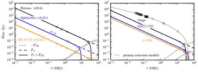
Figure 9: Spectra of three RMHs (left) and three predicted radio micro halos (right). The data for the RMHs are taken from Sijbring (1993, Perseus), Murgia et al. (2010, Ophiuchus) and Giacintucci et al. (2014, RX J1532), and the data for M87 is taken from the halo region of de Gasperin et al. (2012); the grey spectrum is the modelled primary synchrotron emission, assuming a continuous injection that was switched off after a certain time (de Gasperin et al., 2012; Pfrommer, 2013). Dashed lines correspond to unattenuated RMH fluxes, scaled to the 1.4 GHz flux by a scaling factor indicated in the left-hand panel. Dotted lines show the negative flux decrement due to the thermal Sunyaev–Zel’dovich effect. This induces a cut-off to the observable radio spectrum, indicated by the solid lines.

In Fig. 9, we compare the resulting spectra of observed RMHs and the predicted radio micro halos. Dashed lines show the unattenuated radio fluxes, scaled to the 1.4 GHz flux by a scaling factor indicated in the left-hand panel. Dotted lines show the negative flux decrement due to the thermal Sunyaev–Zel’dovich effect, which we determine as in Enßlin (2002). This induces a cut-off to the observable RMH spectra, indicated by the solid lines. The radio micro halo of M87 (black data points from de Gasperin et al., 2012) is presumably generated by primary accelerated CR electrons that have escaped from the bubbles. This component was modelled assuming a continuous injection that was switched off after a certain time (grey solid line). This causes the spectrum to drop exponentially above a break frequency, which corresponds to the cooling time since the switch-off. Despite the harder intrinsic spectrum of the hadronically induced secondary component (black solid line) in comparison to the convex curvature of the primary component, the presence of the Sunyaev–Zel’dovich cut-off precludes a detection of the subdominant hadronic component in M87.

There is a significant range of radio mini and micro halo fluxes (Figs 3 and 9). Especially the comparably tight range of RMH redshifts and thus luminosity distances also implies a range in luminosities. This matches our picture in which RMHs serve as sign posts of the upper end of a continuous sequence in cooling properties. The observed range of gas densities and CR pressures causes the observed diversity of radio luminosities.

6 Conclusions

CR heating has recently re-emerged as an attractive scenario for mediating energetic feedback by AGNs at the centres of galaxy clusters (Guo & Oh, 2008; Enßlin et al., 2011; Fujita & Ohira, 2011; Wiener et al., 2013; Pfrommer, 2013). However, all theoretical studies to date have concentrated on individual objects or a very small sample size, precluding statistically sound conclusions on any heating model.

In this sequence of two papers, we have selected a rich sample of 39 CC clusters and found steady-state solutions of the hydrodynamic equations coupled to the CR energy equation. In those, radiative cooling is balanced by thermal conduction at large scales and by CR heating in the central regions.

We find that those solutions are ruled out in a subsample of clusters that host RMHs because the predicted hadronically induced non-thermal emission exceeds observational radio and (some) gamma-ray data. On the contrary, the predicted non-thermal emission respects observational radio data in CC clusters without RMHs (with the exception of A 383 and A 85, in which the CR-heating solution is barely ruled out). Those non-RMH clusters show exceptionally large AGN radio fluxes, which should be accompanied by an abundant injection of CRs and – by extension – should give rise to a large CR heating rate.

This enables us for the first time to put forward a statistically rooted, self-regulated model of AGN feedback. We propose that non-RMH clusters are heated by streaming CRs homogeneously throughout the cooling region through the generation and dissipation of Alfvén waves. On the contrary, CR heating appears to be insufficient to fully balance the enhanced cooling in RMH clusters. These clusters are also characterized by large SFRs, questioning the presence of a stable heating mechanism that balances the cooling rate. In those systems, thermal conduction should still regulate radiative cooling on large scales, which however is unable to adjust to local thermal fluctuations in the cooling rate because of the strong temperature dependence of the conductivity and may give rise to local thermal instability. However, there will still be some residual level of CR heating in those cooling systems that quenches radiative cooling but is not able to completely offset it.

We emphasize that our self-regulation scenario of CR-induced heating not only predicts stably heated clusters and cooling clusters with abundant star formation, but also systems transitioning from one state to the other, a prominent example of which appears to be the Perseus cluster.

We predict radio micro halos of scales up to a few kpcs surrounding the AGNs of these CR-heated clusters, resembling the diffuse radio emission around Virgo’s central galaxy, M87. Once the CR population has streamed sufficiently far from the centre, it has lost enough energy so that its heating rate is unable to balance radiative cooling any more. As a result star formation increases in clusters that we empirically identify to host an RMH. We suggest that the CR population that has heated the cluster core in the past is now injecting secondary electrons that power the RMH.

Our new picture makes a number of novel predictions that allow scrutinizing it.

1. We predict the presence of radio micro halos associated with all CC clusters that host no classic RMH and have small SFRs (or alternatively H$\alpha$ luminosities, Voit et al., 2008). While this secondary emission component is expected to have a harder spectrum in comparison to the convexly curved, primary radio emission, we find that the negative flux decrement owing to the thermal Sunyaev–Zel’dovich effect typically cuts these emission components off at high frequencies ($\nu\gtrsim 10-50$ GHz). In Virgo, the primary emission component predominates the hadronically induced secondary emission at all observable radio emission frequencies. Hence, we envision the harder secondary emission to predominate the primary component only in those cases where the latter has already cooled sufficiently down, i.e., at late times after the release of the CR electrons from the bubbles or at larger cluster-centric radii.

2. We predict an observable steady-state gamma-ray signal resulting from hadronic CR interactions with the ICM. The spectral index that is expected to be correlated to the injection (electron and proton) index that can be probed at small radii with low-frequency radio observations (Pfrommer, 2013).

Future magneto-hydrodynamic, three-dimensional cosmological simulations that follow CR physics are necessary to study possible time-dependent effects of the suggested scenario such as the impact of CR duty cycles on the heating rates and to address non-spherical geometries associated with the rising AGN bubbles.

Appendix A Density fits

In Table 4 we list the fit parameters of the density profile for the 24 clusters for which we performed our own fits.

Table 4: Parameters for density profiles.

Cluster	$r_{\mathrm{cut,}n_{\mathrm{e}}}^{\mathrm{(1)}}$	$n_{0}$	$\beta$	$r_{\mathrm{c}}$
	(kpc)	($\mathrm{cm}^{-3}$)		(kpc)
Centaurus	62	0.225	0.30	0.9
Hydra A	296	0.067	0.40	11.2
Virgo	44	0.230	0.29	0.6
A 85	248	0.089	0.34	7.2
A 496	79	0.088	0.32	4.9
A 539	311	0.068	0.24	0.5(2)
A 1644	284	0.051	0.26	2.1
A 2052	112	0.027	0.41	18.7
A 2199	84	0.101	0.25	2.2
A 2597	87	0.083	0.43	17.0
A 3112	226	0.079	0.40	10.2
A 3581	105	0.043	0.39	6.9
A 4059	213	0.053	0.29	3.9
AWM 7	78	0.113	0.22	0.5(2)
MKW 3S	386	0.027	0.45	21.9
PKS 0745	496	0.112	0.52	28.0
ZwCl 1742	343	0.029	0.56	30.3
Ophiuchus	257	0.463	0.26	0.5(2)
Perseus	114	0.049	0.62	42.4
2A 0335	148	0.095	0.45	12.0
RBS 797	537	0.101	0.65	43.2
RX J1347	988	0.103	0.65	54.3
RX J1504	587	0.163	0.62	31.8
RX J1532	477	0.091	0.62	38.9

• (1) Maximal radius that we include in fit.

• (2) Parameter fixed during the fit.

Appendix B Calculate non-thermal emission

B.1 Radio emission

We calculate the radio emission from secondary electrons following Pfrommer et al. (2008). Therefore, we model the CR proton population as

$$f_{\mathrm{p}}(p_{\mathrm{p}})=\frac{\mathrm{d}N}{\mathrm{d}p_{\mathrm{p}}\mathrm{d}V}=C_{\mathrm{p}}p_{\mathrm{p}}^{-\alpha_{\mathrm{p}}}\theta(p_{\mathrm{p}}-q_{\mathrm{p}})$$ (16)

where $p_{\mathrm{p}}=P_{\mathrm{p}}/(m_{\mathrm{p}}c)$ is the dimensionless proton momentum. The CR spectrum is a power law in momentum with spectral index $\alpha_{\mathrm{p}}=2.4$. $\theta(x)$ denotes the Heaviside step function, which imposes a lower momentum cut-off at $q_{\mathrm{p}}=0.5$. $C_{\mathrm{p}}$ describes the normalization, which we obtain from the CR pressure as (Enßlin et al., 2007; Pfrommer et al., 2008)

$$C_{\mathrm{p}}(r)=\frac{6P_{\mathrm{cr,ex}}(r)}{m_{\mathrm{p}}c^{2}}\left[\mathcal{B}_{\frac{1}{1+q_{\mathrm{p}}^{2}}}\left(\frac{\alpha_{\mathrm{p}}-2}{2},\frac{3-\alpha_{\mathrm{p}}}{2}\right)\right]^{-1}.$$ (17)

Here, $\mathcal{B}_{x}(a,b)$ denotes the incomplete beta function and we use the extrapolated CR pressure profile, $P_{\mathrm{cr,ex}}(r)$, from the steady state solutions (see Equation 5).

This CR population interacts hadronically with the nucleons in the ICM and produces pions. The charged pions decay into muons and eventually into electrons. The resulting electron distribution in steady state, where hadronic injection balances radiative cooling, can again be described by a power-law spectrum in momentum with spectral index $\alpha_{\mathrm{e}}=\alpha_{\mathrm{p}}+1$. The resulting synchrotron emissivity at frequency $\nu$ per steradian by a secondary population of CR electrons with an isotropic distribution of pitch angles is given by

$$j_{\nu}=\frac{A_{\nu}}{4\pi}C_{\mathrm{p}}n_{\mathrm{N}}\frac{e_{B}}{e_{B}+e_{\mathrm{rad}}}\left(\frac{e_{B}}{e_{B_{\mathrm{c}}}}\right)^{\left(\alpha_{\nu}-1\right)/2}$$ (18)

where $C_{\mathrm{p}}$ is the normalization of the proton spectrum and $n_{\mathrm{N}}=n_{\mathrm{H}}+4n_{\mathrm{He}}=\rho/m_{\mathrm{p}}$ the nucleon number density. The nucleon number density is related to the electron number density by $n_{\mathrm{N}}=\mu_{\mathrm{e}}n_{\mathrm{e}}$. We use our fits to the ACCEPT data to describe $n_{\mathrm{e}}$ (see Section 2.2) and a mean molecular weight per electron of $\mu_{\mathrm{e}}=1.18$. This corresponds to a composition of the ICM with hydrogen mass fraction $X=0.7$ and helium mass fraction $Y=0.28$.

The quantities $e_{B}$, $e_{\mathrm{rad}}$ and $e_{B_{\mathrm{c}}}$ describe the energy densities that are relevant for synchrotron radiation. $e_{B}=B^{2}/(8\pi)$ denotes the magnetic energy density that we parametrize in equation 8. Inverse Compton scattering on radiation fields cools the electron population and is thus important for determining its steady state distribution. The total radiation field in galaxy clusters is composed of CMB photons and the emission from dust and stars such that $e_{\mathrm{rad}}=e_{\mathrm{CMB}}+e_{\mathrm{SD}}$. Here, we treat the energy density of CMB photons with an equivalent magnetic field of $B_{\mathrm{CMB}}=3.24(1+z)^{2}\mathrm{~{}\mu G}$ (Pfrommer et al., 2008). For the emission from stars and dust, we employ the model by Pinzke et al. (2011).

In Fig. 10 we show radial profiles of $e_{B}$, $e_{\mathrm{CMB}}$ and $e_{\mathrm{SD}}$ for our entire cluster sample. At small radii the SD radiation energy density predominates and starts to fall below the magnetic energy density at radii ranging from 20 to 40 kpc, depending on the particular cluster. Because we are looking at nearby clusters ($z<0.45$) and use a comparably strong magnetic field, which is in agreement with Faraday rotation measurements of CCs, the energy density of the CMB never predominates in the core region ($r<100$ kpc) and remains subdominant out to radii of 200 kpc for most clusters.

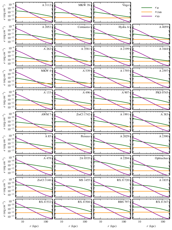
Figure 10: Energy density profiles of the magnetic field, the CMB, and the radiation field emitted by stars and dust. The clusters are ordered by row, starting with non-RMH clusters and followed by RMH-hosting clusters from Perseus onward.

The frequency dependence of the synchrotron emission is encapsulated in $e_{B_{\mathrm{c}}}=B_{\mathrm{c}}^{2}/(8\pi)$ where $B_{\mathrm{c}}=31\nu\mathrm{~{}GHz^{-1}\mu G}$. The index $\alpha_{\nu}$ is related to the spectral index of the electron distribution by $\alpha_{\nu}=(\alpha_{\mathrm{e}}-1)/2$.

The remaining constant $A_{\nu}$ is given by

$$A_{\nu}=4\pi A_{\mathrm{E}_{\mathrm{synch}}}\frac{16^{2-\alpha_{\mathrm{e}}}\sigma_{\mathrm{pp}}m_{\mathrm{e}}c^{2}}{(\alpha_{\mathrm{e}}-2)\sigma_{\mathrm{T}}e_{B_{\mathrm{c}}}}\left(\frac{m_{\mathrm{p}}}{m_{\mathrm{e}}}\right)^{\alpha_{\mathrm{e}}-2}\left(\frac{m_{\mathrm{e}}c^{2}}{\mathrm{GeV}}\right)^{\alpha_{\mathrm{e}}-1}$$ (19)

with the Thomson cross-section $\sigma_{\mathrm{T}}$ and the effective proton–proton cross-section $\sigma_{\mathrm{pp}}$, which is described as (Pfrommer & Enßlin, 2004b)

$$\sigma_{\mathrm{pp}}=32\left(0.96+\mathrm{e}^{4.4-2.4(\alpha_{\mathrm{e}}-1)}\right).$$ (20)

$A_{\mathrm{E}_{\mathrm{synch}}}$ is given by

$$A_{\mathrm{E}_{\mathrm{synch}}}=\frac{\sqrt{3\pi}}{32\pi}\frac{B_{\mathrm{c}}e^{3}}{m_{\mathrm{e}}c^{2}}\frac{\alpha_{\mathrm{e}}+\frac{7}{3}}{\alpha_{\mathrm{e}}+1}\frac{\Gamma\left(\frac{3\alpha_{\mathrm{e}}-1}{12}\right)\Gamma\left(\frac{3\alpha_{\mathrm{e}}+7}{12}\right)\Gamma\left(\frac{\alpha_{\mathrm{e}}+5}{4}\right)}{\Gamma\left(\frac{\alpha_{\mathrm{e}}+7}{4}\right)}.$$ (21)

B.2 Gamma-ray emission

The source density for gamma-rays from pion decay as a function of energy is denoted by $s_{\gamma}(E_{\gamma})$. Thus, the number of photons emitted per unit time and area between the energies $E_{1}$ and $E_{2}$ is given by

$$\begin{split}\lambda_{\gamma}&=\int_{E_{1}}^{E_{2}}\mathrm{d}E_{\gamma}s_{\gamma}(E_{\gamma})\\ &=\frac{4C_{\mathrm{p}}}{3\alpha_{\mathrm{p}}\delta_{\gamma}}\frac{m_{\pi^{0}}c\sigma_{\mathrm{pp}}n_{\mathrm{N}}}{m_{\mathrm{p}}}\left(\frac{m_{\mathrm{p}}}{2m_{\pi^{0}}}\right)^{\alpha_{\mathrm{p}}}\left[\mathcal{B}_{x}\left(\frac{\alpha_{\mathrm{p}}+1}{2\delta_{\gamma}},\frac{\alpha_{\mathrm{p}}-1}{1\delta_{\gamma}}\right)\right]_{x_{1}}^{x_{2}}.\end{split}$$ (22)

In the last step, we have substituted the source function with the detailed description from Pfrommer et al. (2008), which assumes that the CR population can be described as in Equation (16). The source function depends primarily on the normalization of the CR population, $C_{\mathrm{p}}(r)$, and the target density, $n_{\mathrm{N}}(r)$. As described in the case of the radio emissivity, we obtain $C_{\mathrm{p}}(r)$ from the CR pressure profile and $n_{\mathrm{N}}(r)$ from fits to observational data. We adopt a spectral index for the CR proton population of $\alpha_{\mathrm{p}}=2.4$. The shape factor $\delta_{\gamma}$ depends on the spectral index and is given by

$$\delta_{\gamma}\approx 0.14\alpha_{\mathrm{p}}^{-1.6}+0.44.$$ (23)

The effective proton–proton cross-section $\sigma_{\mathrm{pp}}$ is the same as in Equation (20). The neutral pion and proton masses are denoted by $m_{\pi^{0}}$ and $m_{\mathrm{p}}$, respectively. The last factor contains the incomplete beta function $\mathcal{B}_{x}(a,b)$ and is evaluated at $x_{1}$ and $x_{2}$ with

$$x_{i}=\left[1+\left(\frac{m_{\pi^{0}}c^{2}}{2E_{i}}\right)^{2\delta_{\gamma}}\right]^{-1}.$$ (24)

Luminosities and fluences are obtained via Equations (13) and (14), respectively.

Appendix C Non-thermal luminosities

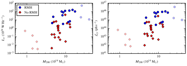
Figure 11: Scaling relations of hadronically induced non-thermal luminosities and cluster masses. We show the 1.4 GHz radio luminosity due to secondary electrons (left) and the pion-decay gamma-ray luminosity above 1 GeV (right). Clusters hosting an RMH (shown with blue circles) populate the upper envelope of these relations. Clearly, both luminosities scale with cluster mass. However, there is an enormous scatter in non-thermal luminosity at fixed mass due to the large variance in gas density across our sample. The latter effect dominates the variance of non-thermal luminosities in our core sample (shown with full colours).

We show scaling relations of hadronically induced non-thermal luminosities and cluster masses in Fig. 11. We show separately radio luminosities emitted by secondary CR electrons and gamma-ray emission due to decaying neutral pions. Assuming that CRs are accelerated at cosmological structure formation shocks during cosmic history and advectively transported into clusters, the non-thermal cluster luminosity scales with the virial mass of clusters as $M_{200}^{\alpha_{M}}$ with $\alpha_{M}\approx 1.4$ (Pfrommer, 2008; Pinzke et al., 2011, excluding the signal from the cluster galaxies). We find a similarly strong scaling with cluster mass. However, this scaling with cluster mass is accompanied with an enormous scatter in non-thermal luminosity at fixed mass due to the large variance in gas density across our sample. The latter effect dominates the variance of non-thermal luminosities in our core sample.

To understand the origin of this scatter, we examine the scaling of the non-thermal luminosity, $\mathcal{L}_{\mathrm{nt}}\propto\int P_{\mathrm{cr}}nf(B)\mathrm{d}V=\int X_{\mathrm{cr}}n^{2}kTf(B)\mathrm{d}V$, where $f(B)=1$ for the gamma-ray luminosity and $f(B)$ represents a weak function of magnetic field strength in the synchrotron-dominated emission regime, i.e., for $e_{B}\gg e_{\mathrm{rad}}$ (equation 18). In Fig. 6, we found a similar spread of $n$ and $X_{\mathrm{cr}}$ of a factor of about $30$ in our entire sample. Hence, we expect $\mathcal{L}_{\gamma}$ to vary by a factor of about $3\times 10^{4}$, which is only marginally reduced to $10^{4}$ if we restrict ourselves to the core sample, despite the tight restriction in cluster mass of this subsample.

There is little difference between the relations for the radio and gamma-ray luminosities, implying that the CR electrons are primarily cooling in the strong synchrotron regime for which $f(B)$ depends only weakly on magnetic field strength. Finally, clusters hosting an RMH populate the upper envelope of these relations since they signal the CC systems with the highest density (at fixed radius, see Fig. 6). The median values of the distribution of RMH cluster and those without RMHs vary by more than an order of magnitude.

References

- Abdo et al. (2009) Abdo A. A., et al., 2009, ApJ, 707, 55
- Ackermann et al. (2010) Ackermann M., et al., 2010, ApJ, 717, L71
- Ackermann et al. (2014) Ackermann M., et al., 2014, ApJ, 787, 18
- Ahnen et al. (2016) Ahnen M. L., et al., 2016, A&A, 589, A33
- Aleksić et al. (2012) Aleksić J., et al., 2012, A&A, 541, A99
- Alexander & Leahy (1987) Alexander P., Leahy J. P., 1987, MNRAS, 225, 1
- Bîrzan et al. (2004) Bîrzan L., Rafferty D. A., McNamara B. R., Wise M. W., Nulsen P. E. J., 2004, ApJ, 607, 800
- Blanton et al. (2003) Blanton E. L., Sarazin C. L., McNamara B. R., 2003, ApJ, 585, 227
- Böhringer et al. (1994) Böhringer H., Briel U. G., Schwarz R. A., Voges W., Hartner G., Trümper J., 1994, Nature, 368, 828
- Brüggen & Kaiser (2002) Brüggen M., Kaiser C. R., 2002, Nature, 418, 301
- Cavagnolo et al. (2009) Cavagnolo K. W., Donahue M., Voit G. M., Sun M., 2009, ApJS, 182, 12
- Chandran & Rasera (2007) Chandran B. D. G., Rasera Y., 2007, ApJ, 671, 1413
- Churazov et al. (2001) Churazov E., Brüggen M., Kaiser C. R., Böhringer H., Forman W., 2001, ApJ, 554, 261
- Coble et al. (2007) Coble K., et al., 2007, AJ, 134, 897
- Colafrancesco & Marchegiani (2008) Colafrancesco S., Marchegiani P., 2008, A&A, 484, 51
- Condon et al. (1998) Condon J. J., Cotton W. D., Greisen E. W., Yin Q. F., Perley R. A., Taylor G. B., Broderick J. J., 1998, AJ, 115, 1693
- Donahue et al. (2007) Donahue M., Sun M., O’Dea C. P., Voit G. M., Cavagnolo K. W., 2007, AJ, 134, 14
- Dutson et al. (2013) Dutson K. L., White R. J., Edge A. C., Hinton J. A., Hogan M. T., 2013, MNRAS, 429, 2069
- Enßlin (2002) Enßlin T. A., 2002, A&A, 396, L17
- Enßlin et al. (2007) Enßlin T. A., Pfrommer C., Springel V., Jubelgas M., 2007, A&A, 473, 41
- Enßlin et al. (2011) Enßlin T., Pfrommer C., Miniati F., Subramanian K., 2011, A&A, 527, A99
- Ettori et al. (2010) Ettori S., Gastaldello F., Leccardi A., Molendi S., Rossetti M., Buote D., Meneghetti M., 2010, A&A, 524, A68
- Fabian et al. (2003) Fabian A. C., Sanders J. S., Allen S. W., Crawford C. S., Iwasawa K., Johnstone R. M., Schmidt R. W., Taylor G. B., 2003, MNRAS, 344, L43
- Fabian et al. (2006) Fabian A. C., Sanders J. S., Taylor G. B., Allen S. W., Crawford C. S., Johnstone R. M., Iwasawa K., 2006, MNRAS, 366, 417
- Fabian et al. (2017) Fabian A. C., Walker S. A., Russell H. R., Pinto C., Sanders J. S., Reynolds C. S., 2017, MNRAS, 464, L1
- Feretti et al. (2012) Feretti L., Giovannini G., Govoni F., Murgia M., 2012, A&ARv, 20, 54
- Fujita & Ohira (2011) Fujita Y., Ohira Y., 2011, ApJ, 738, 182
- Fujita & Ohira (2012) Fujita Y., Ohira Y., 2012, ApJ, 746, 53
- Fujita & Ohira (2013) Fujita Y., Ohira Y., 2013, MNRAS, 428, 599
- Gaspari et al. (2012) Gaspari M., Brighenti F., Temi P., 2012, MNRAS, 424, 190
- Giacintucci et al. (2014) Giacintucci S., Markevitch M., Venturi T., Clarke T. E., Cassano R., Mazzotta P., 2014, ApJ, 781, 9
- Guo & Mathews (2010) Guo F., Mathews W. G., 2010, ApJ, 717, 937
- Guo & Mathews (2011) Guo F., Mathews W. G., 2011, ApJ, 728, 121
- Guo & Oh (2008) Guo F., Oh S. P., 2008, MNRAS, 384, 251
- Guo & Oh (2009) Guo F., Oh S. P., 2009, MNRAS, 400, 1992
- Hillel & Soker (2016) Hillel S., Soker N., 2016, MNRAS, 455, 2139
- Hitomi Collaboration et al. (2016) Hitomi Collaboration et al., 2016, Nature, 535, 117
- Hoffer et al. (2012) Hoffer A. S., Donahue M., Hicks A., Barthelemy R. S., 2012, ApJS, 199, 23
- Hudson et al. (2010) Hudson D. S., Mittal R., Reiprich T. H., Nulsen P. E. J., Andernach H., Sarazin C. L., 2010, A&A, 513, A37
- Jacob & Pfrommer (2017) Jacob S., Pfrommer C., 2017, MNRAS, 467, 1449
- Kannan et al. (2016) Kannan R., Vogelsberger M., Pfrommer C., Weinberger R., Springel V., Hernquist L., Puchwein E., Pakmor R., 2016, preprint, (arXiv:1612.01522)
- Kim & Narayan (2003) Kim W.-T., Narayan R., 2003, ApJ, 596, L139
- Kuchar & Enßlin (2011) Kuchar P., Enßlin T. A., 2011, A&A, 529, A13
- Kulsrud & Pearce (1969) Kulsrud R., Pearce W. P., 1969, ApJ, 156, 445
- Laganá et al. (2013) Laganá T. F., Martinet N., Durret F., Lima Neto G. B., Maughan B., Zhang Y.-Y., 2013, A&A, 555, A66
- Landry et al. (2013) Landry D., Bonamente M., Giles P., Maughan B., Joy M., Murray S., 2013, MNRAS, 433, 2790
- Loewenstein et al. (1991) Loewenstein M., Zweibel E. G., Begelman M. C., 1991, ApJ, 377, 392
- Markevitch & Vikhlinin (2007) Markevitch M., Vikhlinin A., 2007, Phys. Rep., 443, 1
- McNamara et al. (2005) McNamara B. R., Nulsen P. E. J., Wise M. W., Rafferty D. A., Carilli C., Sarazin C. L., Blanton E. L., 2005, Nature, 433, 45
- Murgia et al. (2009) Murgia M., Govoni F., Markevitch M., Feretti L., Giovannini G., Taylor G. B., Carretti E., 2009, A&A, 499, 679
- Murgia et al. (2010) Murgia M., Eckert D., Govoni F., Ferrari C., Pandey-Pommier M., Nevalainen J., Paltani S., 2010, A&A, 514, A76
- Nulsen & Böhringer (1995) Nulsen P. E. J., Böhringer H., 1995, MNRAS, 274, 1093
- Nulsen et al. (2005) Nulsen P. E. J., McNamara B. R., Wise M. W., David L. P., 2005, ApJ, 628, 629
- O’Dea et al. (2008) O’Dea C. P., et al., 2008, ApJ, 681, 1035
- Ogrean et al. (2010) Ogrean G. A., Hatch N. A., Simionescu A., Böhringer H., Brüggen M., Fabian A. C., Werner N., 2010, MNRAS, 406, 354
- Peterson & Fabian (2006) Peterson J. R., Fabian A. C., 2006, Phys. Rep., 427, 1
- Pfrommer (2008) Pfrommer C., 2008, MNRAS, 385, 1242
- Pfrommer (2013) Pfrommer C., 2013, ApJ, 779, 10
- Pfrommer & Enßlin (2004a) Pfrommer C., Enßlin T. A., 2004a, MNRAS, 352, 76
- Pfrommer & Enßlin (2004b) Pfrommer C., Enßlin T. A., 2004b, A&A, 413, 17
- Pfrommer et al. (2008) Pfrommer C., Enßlin T. A., Springel V., 2008, MNRAS, 385, 1211
- Pfrommer et al. (2012) Pfrommer C., Chang P., Broderick A. E., 2012, ApJ, 752, 24
- Pfrommer et al. (2017) Pfrommer C., Pakmor R., Schaal K., Simpson C. M., Springel V., 2017, MNRAS, 465, 4500
- Pinzke & Pfrommer (2010) Pinzke A., Pfrommer C., 2010, MNRAS, 409, 449
- Pinzke et al. (2011) Pinzke A., Pfrommer C., Bergström L., 2011, Phys. Rev. D, 84, 123509
- Reynolds et al. (2015) Reynolds C. S., Balbus S. A., Schekochihin A. A., 2015, ApJ, 815, 41
- Ruszkowski & Begelman (2002) Ruszkowski M., Begelman M. C., 2002, ApJ, 581, 223
- Sarazin (1999) Sarazin C. L., 1999, ApJ, 520, 529
- Sayers et al. (2013) Sayers J., et al., 2013, ApJ, 764, 152
- Shabala et al. (2008) Shabala S. S., Ash S., Alexander P., Riley J. M., 2008, MNRAS, 388, 625
- Sharma et al. (2009) Sharma P., Chandran B. D. G., Quataert E., Parrish I. J., 2009, ApJ, 699, 348
- Sijacki et al. (2008) Sijacki D., Pfrommer C., Springel V., Enßlin T. A., 2008, MNRAS, 387, 1403
- Sijbring (1993) Sijbring L. G., 1993, A radio continuum and HI line study of the perseus cluster
- Simionescu et al. (2012) Simionescu A., et al., 2012, ApJ, 757, 182
- Urban et al. (2011) Urban O., Werner N., Simionescu A., Allen S. W., Böhringer H., 2011, MNRAS, 414, 2101
- Vikhlinin et al. (2006) Vikhlinin A., Kravtsov A., Forman W., Jones C., Markevitch M., Murray S. S., Van Speybroeck L., 2006, ApJ, 640, 691
- Vogt & Enßlin (2005) Vogt C., Enßlin T. A., 2005, A&A, 434, 67
- Voit et al. (2008) Voit G. M., Cavagnolo K. W., Donahue M., Rafferty D. A., McNamara B. R., Nulsen P. E. J., 2008, ApJ, 681, L5
- Wentzel (1971) Wentzel D. G., 1971, ApJ, 163, 503
- Wiener et al. (2013) Wiener J., Oh S. P., Guo F., 2013, MNRAS, 434, 2209
- Yang & Reynolds (2016a) Yang H.-Y. K., Reynolds C. S., 2016a, ApJ, 818, 181
- Yang & Reynolds (2016b) Yang H.-Y. K., Reynolds C. S., 2016b, ApJ, 829, 90
- Zandanel et al. (2014) Zandanel F., Pfrommer C., Prada F., 2014, MNRAS, 438, 124
- Zhuravleva et al. (2014) Zhuravleva I., et al., 2014, Nature, 515, 85
- ZuHone et al. (2013) ZuHone J. A., Markevitch M., Ruszkowski M., Lee D., 2013, ApJ, 762, 69
- de Gasperin et al. (2012) de Gasperin F., et al., 2012, A&A, 547, A56