On the Spectra of Real and Complex Lamé Operators

On the Spectra of Real and Complex Lamé Operators

William A. HAESE-HILL ^†, Martin A. HALLNÄS ^‡ and Alexander P. VESELOV ^†

W.A. Haese-Hill, M.A. Hallnäs and A.P. Veselov

^† Department of Mathematical Sciences, Loughborough University,
^† Loughborough LE11 3TU, UK wahhill@gmail.com, A.P.Veselov@lboro.ac.uk

^‡ Department of Mathematical Sciences, Chalmers University of Technology and
^‡ the University of Gothenburg, SE-412 96 Gothenburg, Sweden hallnas@chalmers.se

Received April 04, 2017, in final form June 21, 2017; Published online July 01, 2017

We study Lamé operators of the form

$$L=-\frac{d^{2}}{dx^{2}}+m(m+1)\omega^{2}\wp(\omega x+z_{0}),$$

with $m\in\mathbb{N}$ and $\omega$ a half-period of $\wp(z)$. For rectangular period lattices, we can choose $\omega$ and $z_{0}$ such that the potential is real, periodic and regular. It is known after Ince that the spectrum of the corresponding Lamé operator has a band structure with not more than $m$ gaps. In the first part of the paper, we prove that the opened gaps are precisely the first $m$ ones. In the second part, we study the Lamé spectrum for a generic period lattice when the potential is complex-valued. We concentrate on the $m=1$ case, when the spectrum consists of two regular analytic arcs, one of which extends to infinity, and briefly discuss the $m=2$ case, paying particular attention to the rhombic lattices.

Lamé operators; finite-gap operators; spectral theory; non-self-adjoint operators

34L40; 47A10; 33E10

1 Introduction

The Lamé equation

$$-\frac{{\rm d}^{2}\psi}{{\rm d}z^{2}}+m(m+1)\wp(z)\psi=\lambda\psi,$$

where $m\in\mathbb{N}$ and $\wp(x)$ is Weierstrass’ elliptic function, satisfying

$$(\wp^{\prime})^{2}=4(\wp-e_{1})(\wp-e_{2})(\wp-e_{3}),$$

is a classical object of 19^th century mathematics.

It surprisingly appeared again at the early age of quantum mechanics in the work by Kramers and Ittmann [15, 16], who discovered that the Lamé equation is closely related to the quantum top by showing that the corresponding Schrödinger equation is separable in the elliptic coordinate system and that the resulting differential equations are of Lamé form (see, e.g., [12]). It is interesting that initially the equation was derived by Gabriel Lamé in 1837 as a result of separation of variables for the Laplace equation in elliptic coordinates, see [17], so one might argue that its origin was quantum from the very beginning.

Viewed as an equation in the complex domain, its solutions, which have a number of remarkable properties, were described explicitly by Hermite and Halphen, see, e.g., [31]. Note that for $x$ on the real line the potential $\wp(x)$ has singularities. If, however, $e_{1}$, $e_{2}$, $e_{3}$ are all real, one can make a pure imaginary half-period shift by $z_{0}=\omega_{3}$ and consider the Lamé operator

$$L=-\frac{{\rm d}^{2}}{{\rm d}x^{2}}+m(m+1)\wp(x+z_{0}),$$ (1.1)

whose potential is real, $2\omega_{1}$-periodic and regular on the whole of $\mathbb{R}$. Consequently, one can apply Bloch–Floquet theory, which implies that the spectrum has a band structure, as described, e.g., in [25].

Generically, the spectrum of a periodic Schrödinger operator (or Hill operator) on the real line consists of a countably infinite number of bands. It was Ince [14] who first pointed out the remarkable fact that the spectrum of $L$ has a band structure with not more than $m$ gaps. Erdélyi [8] later showed that in fact all $m$ gaps are open.

Nowadays, this is just the simplest example in the large class of finite-gap operators discovered in the 1970s, see [7, 18, 21]. It turned out that all such operators can be described explicitly in terms of hyperelliptic Riemann theta functions, with the Lamé operator (1.1) corresponding to the elliptic case. However, it seems that the question of exactly which gaps in the spectrum are open has not been explicitly discussed in the literature even in this case.

The first result of this paper, obtained in Section 2, demonstrates that in the Lamé case it is precisely the first $m$ gaps that are open. Although this fact may not be surprising for experts, we could not find a rigorous proof in the literature. For $m=1$, the result is illustrated in Fig. 1, showing that all the closed gaps are indeed located in the infinite spectral band.

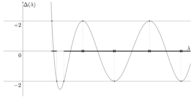
Figure 1: The spectrum of the real Lamé operator (1.1) in the $m=1$ case, where $\Delta(\lambda)$ is the discriminant and crosses denote closed gaps.

In the second part of the paper, we consider the Lamé operator with a complex-valued periodic potential

$$V(x)=m(m+1)\omega^{2}\wp(\omega x+z_{0}),$$ (1.2)

where $\omega$ is any half-period of $\wp(x)$, and the only assumption on $z_{0}\in\mathbb{C}$ is that the corresponding potential is non-singular.

The spectral theory of Schrödinger operators with a complex periodic potential has been studied in a number of papers, see, e.g., [3, 10, 26, 29, 30] as well as references therein. In particular, Rofe-Beketov showed that the spectrum of a Schrödinger operator

$$L=-\frac{{\rm d}^{2}}{{\rm d}x^{2}}+u(x),$$

with periodic, regular, but complex-valued potential $u(x)$ can be defined as the set of $\lambda\in\mathbb{C}$ such that at least one solution of the equation $L\psi=\lambda\psi$ is bounded on the whole real line. Equivalently, the corresponding Floquet multiplier $\rho(\lambda)$, given by

$$\psi(x+T,\lambda)=\rho(\lambda)\psi(x,\lambda),$$

where $T$ is a period of $u(x)$, should lie on the unit circle:

$$|\rho(\lambda)|=1.$$

In the case of the Lamé operator, it follows from work of Gesztesy and Weikard [9, 10, 30], who studied the general elliptic finite-gap case, that the spectrum consists of finitely many regular analytic arcs, with precisely one arc extending to infinity. In the general case of an operator with a periodic complex-valued potential, the question about the relative positions of the spectral arcs was raised earlier by Pastur and Tkachenko [23], who gave an example in which the spectral arcs intersect at interior points. Gesztesy and Weikard [9] observed that more explicit examples are given by the spectrum of the $m=1$ Lamé operator for suitable rhombic period lattices, see also Proposition 3.7 and Figs. 2 and 5 below.

Note that if the shift $z_{0}\neq\omega_{3}$ in the Lamé operator (1.1), we have in general a periodic, regular, but complex-valued potential. However, it is easy to see that the Floquet multipliers do not depend on $z_{0}$, so that the spectrum is the same as in the self-adjoint case. Moreover, setting $\omega=\omega_{1},\omega_{3}$ in (1.2), we have essentially Ince’s result, since the corresponding operator is equivalent to the previous case.

In Section 3, we consider genuinely complex instances of the Lamé operator, concentrating on the simplest case $m=1$. Although this case was briefly discussed earlier in a wider context by Gesztesy and Weikard [9] and Batchenko and Gesztesy [1], we believe that the complete picture is still missing in the literature.

We recall that Hermite’s solutions of the corresponding Lamé equation

$$-\frac{{\rm d}^{2}\psi}{{\rm d}z^{2}}+2\wp(z)\psi=\lambda\psi,\qquad\lambda=-\wp(k),$$

are given by

$$\psi(z,k)=\frac{\sigma(z+k)}{\sigma(z)\sigma(k)}\exp(-\zeta(k)z),$$ (1.3)

where $k\in\mathbb{C}$ and $\sigma(z)$ and $\zeta(z)$ are the Weierstrass $\sigma$- and $\zeta$-function, see, e.g., [31]. Since the solutions have the Floquet property

$$\psi(z+2\omega,k)=\exp(2\eta k-2\zeta(k)\omega)\psi(z,k),$$

with $\eta=\zeta(\omega)$, they remain bounded on the line $z=\omega x+z_{0}$, $x\in\mathbb{R}$, if and only if

$$u(k):=\operatorname{Re}[\eta k-\zeta(k)\omega]=0.$$

By the result of Rofe-Beketov, the corresponding values of $\lambda=-\omega^{2}\wp(k)$ constitute the spectrum of the Lamé operator

$$L=-\frac{{\rm d}^{2}}{{\rm d}x^{2}}+2\omega^{2}\wp(x\omega+z_{0}).$$ (1.4)

Thus, the problem is to study the zero level of the real analytic function $u(k)$, $k\in\mathcal{E}^{\times}=\mathcal{E}\setminus 0$, where $\mathcal{E}={\mathbb{C}}/\mathcal{L}$ is the corresponding elliptic curve.

We show that $u(k)$ is a Morse function on $\mathcal{E}^{\times}$ provided the non-degeneracy conditions

$$\eta+\omega e_{j}\neq 0,\qquad j=1,2,3,$$

are satisfied. We note that this condition also appeared in Takemura’s [28] study of analyticity properties of the eigenvalues of the $m=1$ Lamé operator.

Applying Morse theory arguments we show that, under some additional non-singularity assumptions, the spectrum of (1.4) consists of precisely two non-intersecting regular analytic arcs, with one infinite arc asymptotic to the positive half of the real line shifted by $-2\eta\omega$, and the remaining endpoints being $-\omega^{2}e_{j}$, $j=1,2,3$ (in agreement with [9] and [1]).

The non-degeneracy conditions in general are difficult to control, but in the rhombic case we prove that there exists exactly one exceptional elliptic curve $\mathcal{E}_{*}$ with the value of the $j$-invariant $j_{*}\approx 243.797$ (see the top right corner of Fig. 6 for the corresponding period rhombus). The corresponding spectrum has a tripod structure, see the top right plot in Fig. 2. Note that in this case the spectrum is a union of three simple regular analytic arcs, which is more than usually expected in the $m=1$ case.

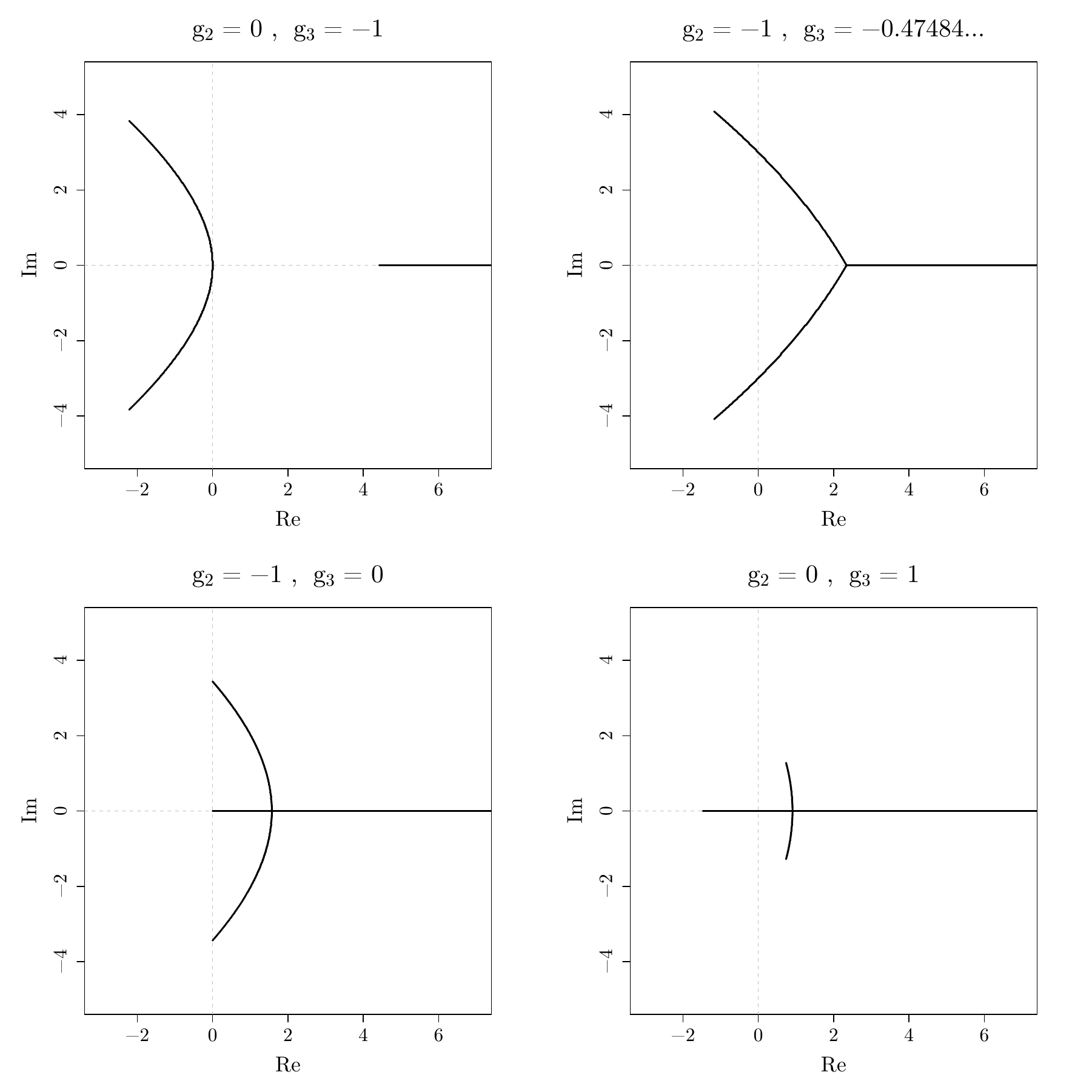
Figure 2: Spectra of the complex Lamé operator (1.4) in rhombic cases with $\omega=\omega_{1}$.

In the rectangular case with $\omega=\omega_{2}$ we show that all closed spectral gaps are contained in the spectral arc extending to infinity. Finally, we briefly discuss the spectrum in the rhombic Lamé case with $m=2$.

2 Spectral gaps for the real Lamé operator

The real Lamé operator (1.1) can be conveniently rewritten in the Jacobian form as

$$L_{m}=-\frac{{\rm d}^{2}}{{\rm d}x^{2}}+m(m+1)k^{2}\operatorname{sn}^{2}(x,k),$$ (2.1)

where $0<k<1$, $m\in\mathbb{N}$ and $\operatorname{sn}(x,k)$ one of the Jacobi elliptic functions, see, e.g., [31].

It is known after Ince [14] and Erdélyi [8] that its spectrum has a band structure with exactly $m$ gaps. We are going to explain now which gaps are open.

Theorem 2.1.

The spectrum of the Lamé operator (2.1) has precisely the first $m$ gaps open.

To prove this we follow the classical approach of Ince [14], which we explain now following [19].

The Lamé potential $m(m+1)k^{2}\operatorname{sn}^{2}(x,k)$ is a real smooth periodic function with period $2K$, where

$$K=\int_{0}^{\pi/2}\frac{{\rm d}\phi}{\sqrt{1-k^{2}\sin^{2}\phi}},$$

so the Lamé operator (2.1) is of Hill type. By the oscillation theorem for Hill operators there exists a sequence of real numbers

$$\lambda_{0}<\lambda^{\prime}_{1}\leq\lambda^{\prime}_{2}<\lambda_{1}\leq\lambda_{2}<\cdots<\lambda^{\prime}_{2n-1}\leq\lambda^{\prime}_{2n}<\lambda_{2n-1}\leq\lambda_{2n}<\cdots,$$ (2.2)

going to infinity, where $\lambda_{j}$ and $\lambda^{\prime}_{j}$ correspond to $2K$-periodic and $2K$-antiperiodic solutions of the Lamé equation

$$-\frac{{\rm d}^{2}\psi}{{\rm d}x^{2}}+m(m+1)k^{2}\operatorname{sn}^{2}(x,k)\psi=\lambda\psi$$ (2.3)

respectively. The intervals $(\lambda_{2n-1},\lambda_{2n})$ and $(\lambda^{\prime}_{2n-1},\lambda^{\prime}_{2n})$ are spectral gaps, and the spectrum of the Lamé operator (2.1) is the complement to the union of these gaps and the interval $(-\infty,\lambda_{0})$. Such a gap is closed if and only if two linearly independent $2K$-periodic or $2K$-antiperiodic solutions of the Lamé equation (2.3) coexist for $\lambda=\lambda_{2n-1}=\lambda_{2n}$ or $\lambda=\lambda^{\prime}_{2n-1}=\lambda^{\prime}_{2n}$, respectively.

So in this language we have to show that all points of coexistence are located in the infinite spectral band.

To prove this we first transform the Lamé equation (2.3) into an equation of Ince’s type

$$(1+a\cos{2\phi})\frac{{\rm d}^{2}y}{{\rm d}\phi^{2}}+b(\sin{2\phi})\frac{{\rm d}y}{{\rm d}\phi}+(c+d\cos{2\phi})y=0,$$ (2.4)

where $a$, $b$, $c$, $d$ are real parameters with $|a|<1$ (see [19]). More precisely, by the substitutions

$$\phi=\operatorname{am}x,$$

where the Jacobi amplitude $\operatorname{am}x=\operatorname{am}(k;x)$ is determined by

$$x=\int_{0}^{\operatorname{am}x}\frac{{\rm d}\phi}{\sqrt{1-k^{2}\sin^{2}\phi}},$$

and $\psi(x)=y(\operatorname{am}x)$, we arrive at (2.4) with

$$a=-b=\frac{k^{2}}{2-k^{2}},\qquad c=\frac{2\lambda-m(m+1)k^{2}}{2-k^{2}},\qquad d=\frac{m(m+1)k^{2}}{2-k^{2}}.$$ (2.5)

Note that $x=2K$ corresponds to $\phi=\pi$, which is reflected in the fact that the coefficients in (2.4) are periodic with period $\pi$.

If Ince’s equation (2.4) has two linearly independent $\pi$-periodic or $\pi$-antiperiodic solutions, then we can find two solutions $y_{1}$, $y_{2}$ such that

$$y_{1}=\sum_{n=0}^{\infty}A_{2n}\cos 2n\phi,\qquad y_{2}=\sum_{n=1}^{\infty}B_{2n}\sin 2n\phi,$$ (2.6)

or

$$y_{1}=\sum_{n=0}^{\infty}A_{2n+1}\cos(2n+1)\phi,\qquad y_{2}=\sum_{n=0}^{\infty}B_{2n+1}\sin(2n+1)\phi.$$ (2.7)

Substituting the periodic series into (2.4) with (2.5), we obtain the recurrence relations

$$\Lambda_{0}A_{0}+P(-1)A_{2}=0,$$ (2.8a)

$$2P(0)A_{0}+\Lambda_{1}A_{2}+P(-2)A_{4}=0,$$ (2.8b)

$$P(n-1)A_{2n-2}+\Lambda_{n}A_{2n}+P(-n-1)A_{2n+2}=0,\qquad n\geq 2$$ (2.8c)

and

$$\Lambda_{1}B_{2}+P(-2)B_{4}=0,$$ (2.9a)

$$P(n-1)B_{2n-2}+\Lambda_{n}B_{2n}+P(-n-1)B_{2n+2}=0,\qquad n\geq 2$$ (2.9b)

where we have introduced

$$P(z)=\frac{m(m+1)k^{2}}{4}-\frac{zk^{2}}{2}-z^{2}k^{2},$$ (2.10)

$$\Lambda_{n}=\lambda-\frac{m(m+1)k^{2}}{2}-\left(1-\frac{k^{2}}{2}\right)4n^{2}.$$ (2.11)

Similarly, the coefficients in the antiperiodic series should satisfy the recurrence relations

$$(P^{*}(0)+\Lambda^{*}_{0})A_{1}+P^{*}(-1)A_{3}=0,$$ (2.12a)

$$P^{*}(n)A_{2n-1}+\Lambda^{*}_{n}A_{2n+1}+P^{*}(-n-1)A_{2n+3}=0,\qquad n\geq 1$$ (2.12b)

and

$$(-P^{*}(0)+\Lambda^{*}_{0})B_{1}+P^{*}(-1)B_{3}=0,$$ (2.13a)

$$P^{*}(n)B_{2n-1}+\Lambda^{*}_{n}B_{2n+1}+P^{*}(-n-1)B_{2n+3}=0,\qquad n\geq 1$$ (2.13b)

with

$$P^{*}(z)=\frac{m(m+1)k^{2}}{4}-\frac{(2z-1)k^{2}}{4}-\frac{(2z-1)^{2}k^{2}}{4},$$ (2.14)

$$\Lambda^{*}_{n}=\lambda-\frac{m(m+1)k^{2}}{2}-\left(1-\frac{k^{2}}{2}\right)(2n+1)^{2}.$$ (2.15)

At this point, we find it convenient to consider even and odd values of $m$ separately. Letting

$$m=2\nu,\qquad\nu\in{\mathbb{Z}}_{\geq 0},$$

we have

$$P(\nu)=P^{*}(-\nu)=0,$$

so that the infinite tridiagonal matrices corresponding to the recurrence relations (2.8)–(2.9) and (2.12)–(2.13) become reducible.

In the periodic case, the finite-dimensional parts of these matrices are

$$K_{\nu,1}=\begin{pmatrix}\Lambda_{0}&P(-1)&0&\cdots&\cdots&0\\ 2P(0)&\Lambda_{1}&P(-2)&0&\cdots&0\\ 0&P(1)&\Lambda_{2}&P(-3)&\cdots&0\\ \vdots&\ddots&\ddots&\ddots&\ddots&\vdots\\ 0&\cdots&0&P(\nu-2)&\Lambda_{\nu-1}&P(-\nu)\\ 0&\cdots&\cdots&0&P(\nu-1)&\Lambda_{\nu}\end{pmatrix}$$ (2.16)

and

$$K_{\nu,2}=\begin{pmatrix}\Lambda_{1}&P(-2)&0&\cdots&0\\ P(1)&\Lambda_{2}&P(-3)&\cdots&0\\ \vdots&\ddots&\ddots&\ddots&\vdots\\ 0&\cdots&P(\nu-2)&\Lambda_{\nu-1}&P(-\nu)\\ 0&\cdots&0&P(\nu-1)&\Lambda_{\nu}\end{pmatrix},$$ (2.17)

which correspond to sequences terminating at $n=\nu$ in the sense that $A_{2n}=B_{2n}=0$ for $n>\nu$.

Introducing the functions

$$\delta_{\nu,1}(\lambda)=\det K_{\nu,1}(\lambda),\qquad\delta_{\nu,2}(\lambda)=\det K_{\nu,2}(\lambda),$$

we let

$$S_{\nu,1}=\{\lambda\colon\delta_{\nu,1}(\lambda)=0\},\qquad S_{\nu,2}=\{\lambda\colon\delta_{\nu,2}(\lambda)=0\},$$

be the sets of corresponding eigenvalues of the Lamé operator (2.1). Recalling (2.10), it is clear that all off-diagonal entries of the matrices $K_{\nu,1}$ and $K_{\nu,2}$ are positive. From the general theory of tridiagonal (Jacobi) matrices (see, e.g., [27]), it follows that $S_{\nu,1}$ and $S_{\nu,2}$ consist of $\nu+1$ respectively $\nu$ real and distinct eigenvalues.

By specializing [19, Theorem 7.3] to the Lamé case, we find that $S_{\nu}:=S_{\nu,1}\cup S_{\nu,2}$ contains the simple part of the periodic spectrum, which we state as the following lemma.

Lemma 2.2.

Let $m=2\nu$, $\nu\in{\mathbb{Z}}_{\geq 0}$. If $\lambda$ belongs to the periodic spectrum of the Lamé operator (2.1) and has multiplicity $1$, then $\lambda\in S_{\nu}$.

Turning to the the antiperiodic case, we note that the recurrence relations (2.12)–(2.13) have no solutions given by terminating sequences. Instead, the relevant finite-dimensional matrices

$$K_{\nu,1}^{*}=\begin{pmatrix}P^{*}(0)+\Lambda^{*}_{0}&P(-1)&0&\cdots&0\\ P^{*}(1)&\Lambda^{*}_{1}&P^{*}(-2)&\cdots&0\\ \vdots&\ddots&\ddots&\ddots&\vdots\\ 0&\cdots&P^{*}(\nu-2)&\Lambda^{*}_{\nu-1}&P^{*}(-\nu+1)\\ 0&\cdots&0&P^{*}(\nu-1)&\Lambda^{*}_{\nu-1}\end{pmatrix}$$ (2.18)

and

$$K_{\nu,2}^{*}=\begin{pmatrix}-P^{*}(0)+\Lambda^{*}_{0}&P(-1)&0&\cdots&0\\ P^{*}(1)&\Lambda^{*}_{1}&P^{*}(-2)&\cdots&0\\ \vdots&\ddots&\ddots&\ddots&\vdots\\ 0&\cdots&P^{*}(\nu-2)&\Lambda^{*}_{\nu-1}&P^{*}(-\nu+1)\\ 0&\cdots&0&P^{*}(\nu-1)&\Lambda^{*}_{\nu-1}\end{pmatrix}$$ (2.19)

are related to sequences with $A_{2\nu-1},B_{2\nu-1}\neq 0$. Indeed, such solutions of the recurrence relations (2.12)–(2.13) exist only if the matrices $K_{\nu,1}^{*}$, $K_{\nu,2}^{*}$ are singular.

Letting

$$\delta_{\nu,1}^{*}(\lambda)=\det K_{\nu,1}^{*}(\lambda),\qquad\delta_{\nu,2}^{*}(\lambda)=\det K_{\nu,2}^{*}(\lambda),$$

we introduce the sets

$$S_{\nu,1}^{*}=\{\lambda\colon\delta_{\nu,1}^{*}(\lambda)=0\},\qquad S_{\nu,2}^{*}=\{\lambda\colon\delta_{\nu,2}^{*}(\lambda)=0\}.$$

Just as in the periodic case, we see that each of the two sets $S_{\nu,j}^{*}$ consists of $\nu$ real and distinct eigenvalues. Moreover, we infer from [19, Theorem 7.4] that $S^{*}_{\nu}:=S^{*}_{\nu,1}\cup S^{*}_{\nu,2}$ contains the simple part of the antiperiodic spectrum.

Lemma 2.3.

Let $m=2\nu$, $\nu\in{\mathbb{Z}}_{\geq 0}$. If $\lambda$ belongs to the antiperiodic spectrum of the Lamé operator (2.1) and has multiplicity $1$, then $\lambda\in S^{*}_{\nu}$.

Since the spectrum of the Lamé operator (2.1) has precisely $m=2\nu$ gaps, the ends of the gaps must be given by the $m$ largest eigenvalues in $S_{\nu}$ and all $m$ eigenvalues in $S^{*}_{\nu}$. (Recall that $(-\infty,\lambda_{0})$ is not counted as a gap.)

We are now ready to complete the proof of Theorem 2.1 for even $m$. From (2.10)–(2.11) and (2.16)–(2.17) it easily follows that

$$\delta_{\nu,j}(k)=\prod_{n=j-1}^{\nu}\big{(}\lambda-(2n)^{2}\big{)}+\mathcal{O}\big{(}k^{2}\big{)},\qquad k\to 0,$$

where $j=1,2$. Similarly, (2.14)–(2.15) and (2.18)–(2.19) readily yield

$$\delta^{*}_{\nu,j}(k)=\prod_{n=0}^{\nu-1}\big{(}\lambda-(2n+1)^{2}\big{)}+\mathcal{O}\big{(}k^{2}\big{)},\qquad k\to 0.$$

This implies that the $m$ gaps close at the points $\lambda=j^{2}$, $j=1,\ldots,m$, as $k\to 0$. On the other hand, taking $k\to 0$ in (2.3), we obtain the free Schrödinger equation $-\psi^{\prime\prime}=\lambda\psi$, and (excluding the constant solution $\psi=1$ with $\lambda=0$) the $m$ smallest values of $\lambda$ for which it has $\pi$-periodic or $\pi$-antiperiodic solutions are precisely $\lambda=j^{2}$, $j=1,\ldots,m$. Using that the eigenvalues $\lambda=\lambda(k)\in S_{\nu}\cup S^{*}_{\nu}$ have multiplicity one, a standard argument shows that they depend analytically on $k$, see e.g. Chapter XII in [24]. Hence there exists $k_{1}\in(0,1)$ such that all points of coexistence are indeed contained in the infinite spectral band for $k\in(0,k_{1})$.

There remains to show that neither of the following two scenarios can occur for $k\geq k_{1}$: first, a point of coexistence crosses one or more open gaps; and, second, an open gap closes while a point of coexistence turns into an open gap. The first scenario is immediately ruled out by the interlacing property (2.2), and the second by the analyticity of the eigenvalues.

This concludes the proof in the case of even $m$. It is straightforward to adapt the arguments above to handle the case of odd $m$. In particular, the roles of the periodic and antiperiodic solutions will then be interchanged, and analogues of Lemmas 2.2–2.3 can once more be obtained from [19, Theorems 7.3–7.4].

Example 2.4.

Consider the simplest nontrivial even case $m=2$, which corresponds to the Lamé operator

$$L_{2}=-\frac{{\rm d}^{2}}{{\rm d}x^{2}}+6k^{2}\operatorname{sn}^{2}(x,k).$$ (2.20)

The edges of its two spectral gaps $(\lambda^{\prime}_{1},\lambda^{\prime}_{2})$ and $(\lambda_{1},\lambda_{2})$, which correspond to the first two eigenvalues $\lambda_{1}^{\prime}$, $\lambda^{\prime}_{2}$ from its antiperiodic spectrum and the second and third eigenvalues $\lambda_{1}$, $\lambda_{2}$ from its periodic spectrum, are easily computed explicitly.

Indeed, observing that

$$\delta^{*}_{1,1}=P^{*}(0)+\Lambda^{*}_{0},\qquad\delta^{*}_{1,2}=-P^{*}(0)+\Lambda^{*}_{0},$$

we find that the edges of the first gap are given by

$$\lambda^{\prime}_{1}=1+k^{2},\qquad\lambda^{\prime}_{2}=1+4k^{2},$$ (2.21)

cf. (2.14)–(2.15). To determine the edges of the second gap, we should find the roots $\lambda$ of the polynomials

$$\delta_{1,1}=\begin{vmatrix}\Lambda_{0}&P_{-1}\\ 2P_{0}&\Lambda_{1}\\ \end{vmatrix},\qquad\delta_{1,2}=\Lambda_{1}.$$

Recalling (2.10)–(2.11), we deduce that the two roots of the former polynomial are

$$\lambda_{0}=2\big{(}1+k^{2}-\sqrt{1-k^{2}+k^{4}}\big{)},\qquad\lambda_{2}=2\big{(}1+k^{2}+\sqrt{1-k^{2}+k^{4}}\big{)},$$ (2.22)

whereas the latter has the single root

$$\lambda_{1}=4+k^{2}.$$ (2.23)

The relevant eigenvalues are plotted together with the ground state eigenvalue from the periodic spectrum in Fig. 3.

In the limit $k\to 1$ the real period goes to infinity and the Lamé potential

$$6k^{2}\operatorname{sn}^{2}(x,k)\to 6-6\operatorname{sech}^{2}x.$$

The potential $u(x)=-6\operatorname{sech}^{2}x$ decays exponentially at infinity and is a special example of a $2$-soliton potential, see, e.g., [6]. The corresponding operator

$$H_{2}=-\frac{{\rm d}^{2}}{{\rm d}x^{2}}-6\operatorname{sech}^{2}x$$

is known to be reflectionless. Its spectrum has continuous part $[0,\infty)$ and discrete part consisting of the two eigenvalues $-1$ and $-4$. Note that for $k\to 1$ the formulae (2.21)–(2.23) show that the two finite spectral bands degenerate to the eigenvalues $\lambda_{0}=\lambda^{\prime}_{1}=2$ and $\lambda^{\prime}_{2}=\lambda_{1}=5$, while $\lambda_{2}\to 6$, in agreement with Fig. 3.

Figure 3: First five eigenvalues from the periodic and antiperiodic spectra of the Lamé operator (2.20).

3 The spectrum of the complex Lamé operator

Let $\mathcal{E}={\mathbb{C}}/\mathcal{L}$ be a general elliptic curve, where $\mathcal{L}$ is a period lattice. To begin with, we do not impose any reality conditions. Let $\wp(z)$ be the corresponding Weierstrass’ elliptic function,

$$\wp(z+\Omega)=\wp(z),\qquad\Omega\in\mathcal{L},$$

which satisfies the equation

$$(\wp^{\prime})^{2}=4(\wp-e_{1})(\wp-e_{2})(\wp-e_{3}),$$

see, e.g., [31]. It has poles of second order at all lattice points, which are the only singularities of $\wp(z)$.

Let $\omega$ be a half-period: $2\omega\in\mathcal{L}$, and consider the complex Lamé operator $L=L(\mathcal{E},\omega,m,z_{0})$ in $L^{2}({\mathbb{R}})$ given by

$$L=-\frac{{\rm d}^{2}}{{\rm d}x^{2}}+m(m+1)\omega^{2}\wp(\omega x+z_{0}),$$ (3.1)

with $m\in\mathbb{N}$ and $z_{0}\in\mathbb{C}$ chosen such that the line $z=\omega x+z_{0}$, $x\in{\mathbb{R}}$, does not contain any points of $\mathcal{L}$. Note that the potential $m(m+1)\omega^{2}\wp(\omega x+z_{0})$ is regular and periodic with period $2$, but is in general complex-valued.

From the work of Rofe-Beketov [26] on the spectral theory of non-self-adjoint differential operators in $L^{2}({\mathbb{R}})$ with complex-valued periodic coefficients, it follows that the spectrum of $L$ can be characterised as the set of $\lambda\in\mathbb{C}$ such that the associated Lamé equation

$$-\frac{{\rm d}^{2}\phi}{{\rm d}x^{2}}+m(m+1)\omega^{2}\wp(\omega x+z_{0})\phi=\lambda\phi,\qquad x\in{\mathbb{R}},$$ (3.2)

has a non-zero bounded solution. Equivalently, the corresponding Floquet multiplier $\mu(\lambda)$, defined by

$$\phi(x+2,\lambda)=\mu(\lambda)\phi(x,\lambda),$$

must have absolute value $|\mu(\lambda)|=1$.

Proposition 3.1.

The spectrum of the complex Lamé operator (3.1) does not depend on the value of $z_{0}$ and is determined by the condition (3.6) below.

Proof.

We will use the classical results about the Lamé equation

$$-\frac{{\rm d}^{2}\psi}{{\rm d}z^{2}}+m(m+1)\wp(z)\psi=\lambda\psi$$ (3.3)

in the complex domain $z\in{\mathbb{C}}$. Its solutions were described by Hermite [13] in the following way, see, e.g., [31, Section 23.7]. First, one notes that the product $X$ of any pair of solutions of (3.3) satisfies the third order equation

$$-\frac{{\rm d}^{3}X}{{\rm d}z^{3}}+4\big{(}m(m+1)\wp(z)-\lambda\big{)}\frac{{\rm d}X}{{\rm d}z}+2m(m+1)\wp^{\prime}(z)=0.$$

Changing variable to

$$\xi=\wp(z)$$

yields the algebraic form of this equation:

$$-4(\xi-e_{1})(\xi-e_{2})(\xi-e_{3})\frac{{\rm d}^{3}X}{{\rm d}\xi^{3}}-3\big{(}6\xi^{2}-g_{2}/2\big{)}\frac{{\rm d}^{2}X}{{\rm d}\xi^{2}}$$

$$\qquad{}+4((m^{2}+m-3)\xi-\lambda)\frac{{\rm d}X}{{\rm d}\xi}-2m(m+1)X=0.$$

Making a power series ansatz in $\xi-e_{2}$ (say), it is straightforward to verify that the Lamé equation (3.3) has two solutions $\psi^{\pm}$ whose product $X$ is a polynomial in $\xi-e_{2}=\wp(z)-e_{2}$ of the form

$$X(\xi)=(\xi-e_{2})^{m}+\sum_{r=1}^{m}c_{r}(\xi-e_{2})^{m-r},$$

with some coefficients $c_{r}\in\mathbb{C}$. This polynomial can be written in the factorised form

$$X(\xi)=\prod_{j=1}^{m}(\xi-\wp(k_{j})),$$

where the $k_{j}=k_{j}(\lambda)\in{\mathbb{C}}$ are determined by this relation up to permutation and up to a sign. Assume now that $\psi^{\pm}$ are linearly independent, so that their Wronskian

$$W\big{(}\psi^{+},\psi^{-}\big{)}\equiv C\neq 0.$$ (3.4)

(Otherwise $\psi^{\pm}$ are one of the $2m+1$ Lamé functions.) The sign of $k_{j}$ can then be fixed by requiring

$$\frac{{\rm d}X}{{\rm d}\xi}\Bigg{\arrowvert}_{\xi=\wp(k_{j})}=\frac{C}{\wp^{\prime}(k_{j})}.$$

Finally, by solving (3.4) and ${\rm d}(\psi^{+}\psi^{-})/{\rm d}z={\rm d}X/{\rm d}z$ for ${\rm d}\log\psi^{\pm}/{\rm d}z$ and integrating, one finds that (3.3) is satisfied by the two functions

$$\psi^{\pm}=\prod_{j=1}^{m}\left(\frac{\sigma(z\pm k_{j})}{\sigma(z)\sigma(k_{j})}\right){\rm e}^{\mp\sum\limits_{j=1}^{m}\zeta(k_{j})z}.$$ (3.5)

Restricting (3.5) to the line $z=\omega x+z_{0}$ and using the quasi-periodicity of the $\sigma$- and $\zeta$-function we see that (3.2) has the Floquet solutions with Floquet multiplier $\mu={\rm e}^{2f_{m}}$,

$$f_{m}(\lambda)=\zeta(\omega)\sum_{j=1}^{m}k_{j}-\omega\sum_{j=1}^{m}\zeta(k_{j}).$$

Since $f_{m}$ is manifestly independent of $z_{0}$, it follows that the spectrum of the complex Lamé operator (3.1), determined by the condition

$$\operatorname{Re}[f_{m}(\lambda)]=0,$$ (3.6)

is indeed independent of the value of $z_{0}$. ∎

Unfortunately, the condition (3.6) is very difficult to analyse in general, so we will now focus on the simplest non-trivial case $m=1$. Hermite’s solutions of (3.3) have the form (1.3):

$$\psi(z,k)=\frac{\sigma(z+k)}{\sigma(z)\sigma(k)}\exp(-\zeta(k)z),$$

with parameter $k$ related to $\lambda$ by $\lambda=-\wp(k)$. Restriction to the line $z=\omega x+z_{0}$ gives the solutions to (3.2) with

$$\lambda=-\omega^{2}\wp(k)$$

and Floquet multiplier given by

$$f(k)=\eta k-\omega\zeta(k).$$

In particular, the corresponding solutions are bounded for $x\in{\mathbb{R}}$ if and only if

$$u(k):=\operatorname{Re}[f(k)]=0.$$ (3.7)

To study the solutions of this transcendental equation we will use elementary Morse theory arguments, see, e.g., [20].

Lemma 3.2.

Assuming that

$$\eta+\omega e_{j}\neq 0,\qquad j=1,2,3,$$ (3.8)

$u(k)$ is a Morse function on $\mathcal{E}^{\times}$, with critical points $\pm k^{*}$ given by

$$\eta+\omega\wp(k^{*})=0.$$

Moreover, the index of $u(k)$ at $k=\pm k^{*}$ is equal to one.

Proof.

Given that $\omega$ is a half-period, there exist $\nu_{1},\nu_{3}\in{\mathbb{Z}}$ such that

$$\omega=\nu_{1}\omega_{1}+\nu_{3}\omega_{3}.$$

By the quasi-periodicity of $\zeta(z)$, we have

$$u(k+2\omega_{j})-f(k)=\nu_{l}\operatorname{Re}[\eta_{l}\omega_{j}-\eta_{j}\omega_{l}],\qquad l\neq j.$$

Hence the Legendre relation $\eta_{1}\omega_{3}-\eta_{3}\omega_{1}=i\pi/2$ ensures that the right-hand side equals zero, so that $u(k)$ is a well-defined function on $\mathcal{E}^{\times}$.

Writing $k=s+it$, the critical points of $u(k)$ are the solutions of $u_{s}=u_{t}=0$, which are equivalent to

$$\frac{{\rm d}f(k)}{{\rm d}k}=\frac{{\rm d}(\eta k-\omega\zeta(k))}{{\rm d}k}=\eta+\omega\wp(k)=0.$$

Since $\wp(k)$ is an even function of order two, this equation has precisely two solutions $k=\pm k^{*}$. Letting

$$v(k)=\operatorname{Im}[f(k)],$$

we infer from the Cauchy–Riemann equations that the Hessian matrix

$$H(u)=\begin{bmatrix}u_{ss}&v_{tt}\\ v_{tt}&-u_{ss}\end{bmatrix},$$

which has eigenvalues

$$\lambda_{\pm}=\pm\sqrt{u_{ss}^{2}+v_{tt}^{2}}.$$

We recall that $u(k)$ is a Morse function if $H(u)$ is non-singular at all of its critical points, with the index being equal to the number of negative eigenvalues. Clearly, $H(u)$ is singular if and only if $u_{ss}=v_{tt}=0$ or, equivalently,

$$\frac{{\rm d}^{2}f(k)}{{\rm d}k^{2}}=\frac{{\rm d}^{2}(\eta k-\omega\zeta(k))}{{\rm d}k^{2}}=\omega\wp^{\prime}(k)=0.$$

Recalling that the only zeros of $\wp^{\prime}(k)$ on $\mathcal{E}^{\times}$ are $k=\omega_{j}$, $j=1,2,3$, we see that $H(u)$ is singular only if $\eta+\omega e_{j}=0$ for some $j=1,2,3$, which is excluded by the assumption (3.8). ∎

Using Morse theory, we can thus determine the topological nature of the zero set (3.7). We assume that (3.8) holds true, so that the critical points of $u(k)$ are non-degenerate, and that the level set $u(k)=0$ is non-singular in the sense that

$$u(k^{*})\neq 0.$$ (3.9)

We note that the lemniscatic case yields an example of a singular level set and the rhombic cases contain singular examples as well as a degenerate level set, see Figs. 5 and 2.

Proposition 3.3.

Under our non-degeneracy and non-singularity assumptions (3.8) and (3.9), the closure $\bar{Z}_{u}\subset\mathcal{E}$ of the zero set

$$Z_{u}=\big{\{}k\in\mathcal{E}^{\times}\colon u(k)=0\big{\}}$$

consists of two simple closed curves in $\mathcal{E}$ representing the same $($non-trivial$)$ homology class.

Proof.

By our non-singularity assumption, we can fix the sign of $k^{*}$ such that

$$c^{*}:=u(k^{*})>0.$$

For $c\in{\mathbb{R}}$, we let $\mathcal{E}_{c}=\overline{\mathcal{E}_{c}^{\times}}\subset\mathcal{E}$ be the closure of the set

$$\mathcal{E}_{c}^{\times}:=\big{\{}k\in\mathcal{E}^{\times}\colon-\infty<u(k)\leq c\big{\}}$$

(where, as we shall see below, taking the closure amounts to adding the point $k=0$).

First, we prove that each $\mathcal{E}_{c}$ with $c<-c^{*}$ is diffeomorphic to a disc. Since the meromorphic function $f(k)=\eta k-\omega\zeta(k)$ is odd and has a simple pole at $k=0$ with residue $-\omega$, we can find neighbourhoods $U,V\ni 0$ and a biholomorphic mapping $g\colon U\to V$ such that

1. $g(0)=0$ and $g^{\prime}(0)=1$,

2. $g(-k)=-g(k)$, $k\in U$,

3. $f\big{(}g^{-1}(z)\big{)}=-\omega/z$, $z\in V$.

Letting

$$\omega=\alpha+i\beta,\qquad z=x+iy,$$

the set $\operatorname{Re}[-\omega/z]\leq c$, $z\neq 0$, is given by

$$\left(x+\frac{\alpha}{2c}\right)^{2}+\left(y+\frac{\beta}{2c}\right)^{2}\leq\frac{\alpha^{2}+\beta^{2}}{4c^{2}},$$ (3.10)

where $(x,y)\neq(0,0)$. By choosing $c^{\prime}<-c^{*}$ sufficiently small, we can ensure that the disc (3.10) is contained within $V$ and therefore that it is diffeomorphic to $\mathcal{E}_{c^{\prime}}$. For $c^{\prime}<c<-c^{*}$, we infer from [20, Theorem 3.1] that $\mathcal{E}_{c}$ is diffeomorphic to $\mathcal{E}_{c^{\prime}}$, and the assertion follows. (To be precise, the theorem does not apply as it stands, since $u(k)$ is not defined at $k=0$. However, $\langle\operatorname{grad}u,\operatorname{grad}u\rangle^{-1}\operatorname{grad}u$ extends to a smooth vector field on a neighbourhood of $\mathcal{E}_{c}$, $c<-c^{*}$, and the construction of the diffeomorphisms $\varphi_{t}\colon\mathcal{E}\to\mathcal{E}$ is readily adapted to the present case.)

Letting $0<\epsilon<c^{*}$, the region $u^{-1}([-c^{*}-\epsilon,-c^{*}+\epsilon])$ contains no critical point of $u$ other than $-k^{*}$. Since the index of $u(k)$ at $k=-k^{*}$ is one, it follows that $\mathcal{E}_{-c^{*}+\epsilon}$ is diffeomorphic to a disc with a thickened $1$-cell attached, cf. [20, Theorem 3.2]. Moreover, increasing $c$ from $-c^{*}+\epsilon$ to $0$ does not alter the diffeomorphism type of $\mathcal{E}_{c}$. Considering the boundary of $\mathcal{E}_{0}$, we thus arrive at the statement. ∎

This leads us to the following result, which can also be extracted from [1, Theorem 1.1 and Example C.1].

Proposition 3.4.

Under our assumptions of non-degeneracy (3.8) and non-singularity (3.9), the spectrum of the complex Lamé operator (3.1) with $m=1$ consists of two regular analytic arcs. Moreover, precisely one arc extends to infinity and the remaining endpoints are $-\omega^{2}e_{j}$, $j=1,2,3$.

Proof.

By Proposition 3.3, there exist simple closed curves $\gamma_{1}$, $\gamma_{2}$ such that

$$\bar{Z}_{u}=\gamma_{1}\cup\gamma_{2}.$$

For each $j=1,2,3$, we deduce from the Legendre relation that $\omega_{j}\in Z_{u}$. In addition, $\bar{Z}_{u}$ contains $k=0$ and is invariant under the reflection $k\to-k$, which implies that each curve $\gamma_{j}$ contains precisely two fixed points. Since the quotient map

$$\mathcal{E}\to\mathcal{E}/(k\to-k)=\mathbb{CP}^{1}$$

is given by $k\mapsto\wp(k)$, the image of $\bar{Z}_{u}$ in $\mathbb{CP}^{1}$ under the map $k\mapsto\lambda=-\omega^{2}\wp(k)$ consists of two regular analytic arcs connecting two pairs of fixed points. ∎

The next proposition, which can also be extracted from [1], describes the asymptotic behaviour of the infinite spectral arc.

Proposition 3.5.

For $m=1$, the spectral arc of the complex Lamé operator (3.1) that extends to infinity is asymptotic to the positive real line shifted by $-2\eta\omega$.

Proof.

Recalling from the proof of Proposition 3.3 the biholomorphic mapping $g\colon U\to V$, we observe that any $z\in V$ satisfying the spectral condition $u\big{(}g^{-1}(z)\big{)}=\operatorname{Re}[-\omega/z]=0$ is of the form

$$z=i\omega s,\qquad s\neq 0.$$

By Properties (1)–(3) of $g$, we have

$$g^{-1}(z)=z-\frac{\eta}{\omega}z^{3}+\mathcal{O}\big{(}z^{5}\big{)}.$$

This implies

$$\lambda=-\omega^{2}\wp\big{(}g^{-1}(i\omega s)\big{)}=\frac{1}{s^{2}}-2\eta\omega+\mathcal{O}\big{(}s^{2}\big{)},\qquad s\to 0,$$

from which the assertion clearly follows. ∎

For the remainder of this section, we restrict attention to real elliptic curves $\mathcal{E}$ given by

$$y^{2}=4x^{3}-g_{2}x-g_{3},\qquad g_{2},g_{3}\in\mathbb{R}.$$

There are two types of such curves, depending on the sign of the discriminant

$$\Delta=g_{2}^{3}-27g_{3}^{2}.$$

If $\Delta>0$, the roots $e_{1}$, $e_{2}$, $e_{3}$ of the polynomial $p(x)=4x^{3}-g_{2}x-g_{3}$ are all real, the corresponding real curve consists of two ovals ($M$-curve) and the period lattice $\mathcal{L}$ is rectangular.

If $\Delta<0$, we have one real root $e_{1}$ and a pair $e_{2}$, $e_{3}$ of complex conjugate roots, $e_{3}=\overline{e_{2}}$. The corresponding real curve consists of one oval and the period lattice $\mathcal{L}$ is rhombic.

We first consider the rectangular case, with basic half-periods

$$\omega_{1}\in(0,\infty),\qquad\omega_{3}\in i(0,\infty).$$ (3.11)

The simplest instance of the corresponding Lamé operator (3.1) that is truly complex is obtained by choosing

$$\omega=\omega_{2}=\omega_{1}+\omega_{3}.$$

For this choice of $\omega$, we have used the software R to numerically compute the spectrum of (3.1) for $g_{3}=1$ and four different values of $g_{2}$. The results are displayed in Fig. 4.

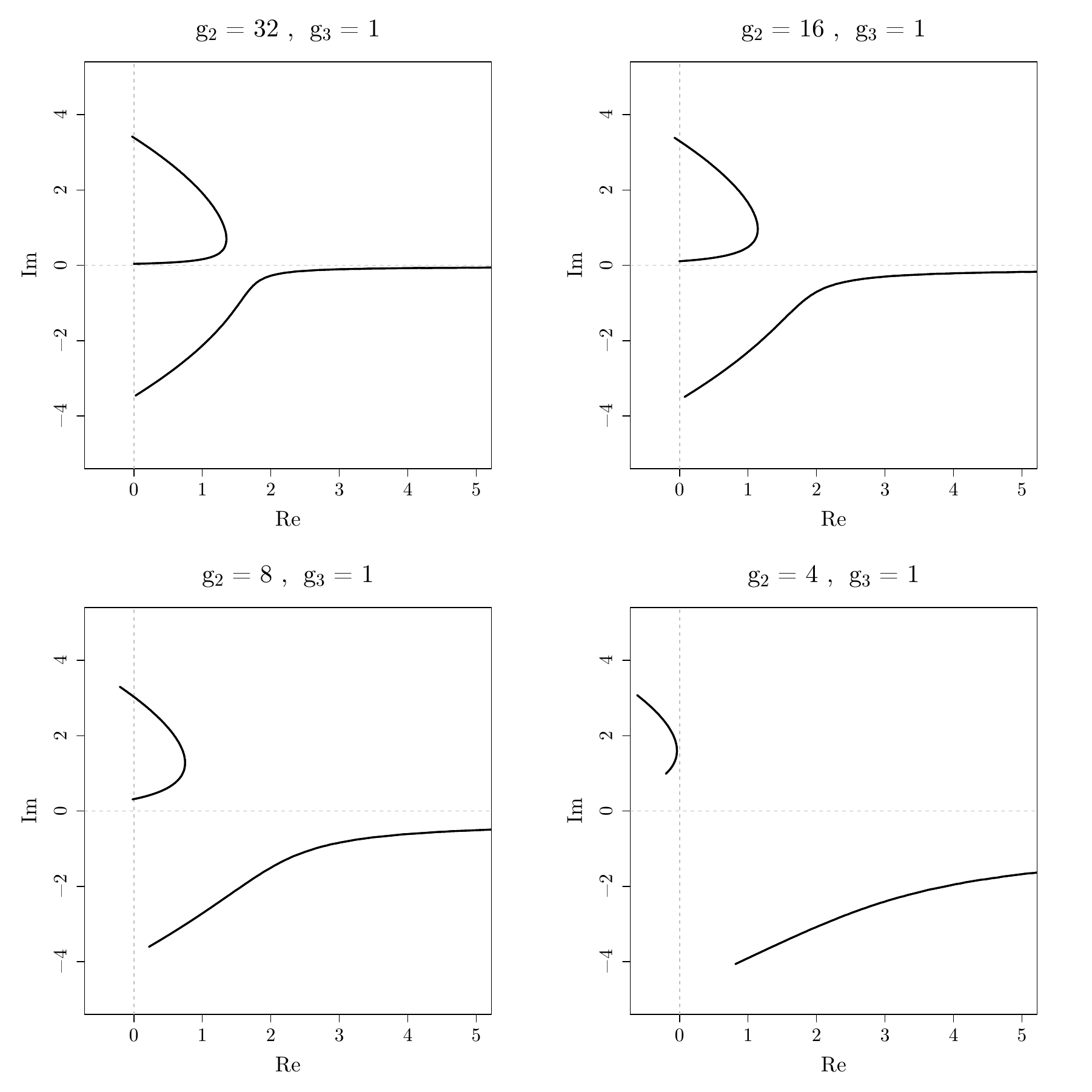
Figure 4: Spectra of the complex Lamé operator (3.1) for rectangular period lattices ${\mathcal{L}}$, $m=1$ and $\omega=\omega_{2}$.

We note that the (anti-)periodic solutions of (3.2) are given by $k\in Z_{u}$ satisfying

$$v(k):=\operatorname{Im}[f(k)]=p\frac{\pi}{2},\qquad p\in\mathbb{Z}.$$ (3.12)

By the Legendre relation, $v(\omega_{3})=-v(\omega_{1})=\pi/2$ and $v(\omega_{2})=0$. Since $\lambda=-\omega^{2}\wp(\omega_{j})$, $j=1,2,3$, at the endpoints of the spectral arcs, the remaining values of $p$ must correspond to points contained in one of the two spectral arcs. Following standard terminology for the real Lamé operator, we call such a point in the spectrum a closed spectral gap. In analogy with Theorem 2.1, we have the following result.

Theorem 3.6.

For $m=1$, $\omega=\omega_{2}$ and $\omega_{1}$, $\omega_{3}$ of the form (3.11), all closed spectral gaps of the complex Lamé operator (3.1) are located on the spectral arc extending to infinity.

Our proof of this result relies on a detailed analysis of the lemniscatic case. The corresponding set $\bar{Z}_{u}$ and spectrum of (3.1) are shown in Fig. 5. The curve $k=(1-i)\omega_{1}s$, $-1\leq s\leq 1$, and spectral arc $[0,\infty)$ are deduced analytically in the proof of Proposition 3.7 below, whereas the remaining curve and spectral arc were obtained numerically using the software R.

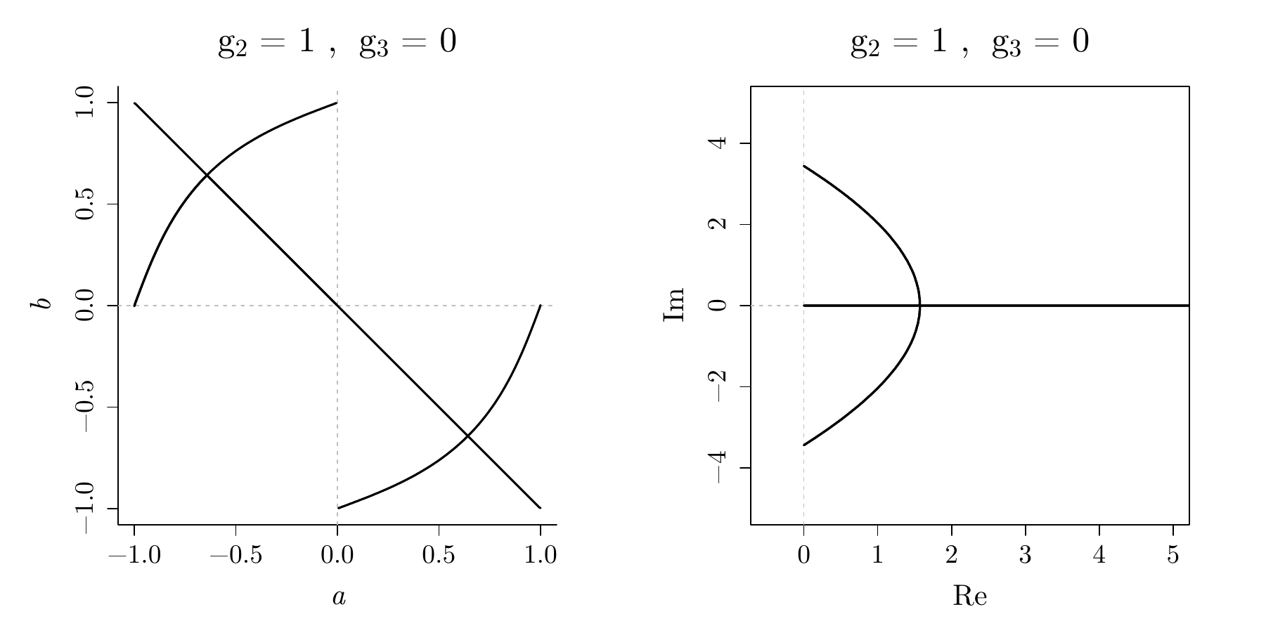
Figure 5: The set $\bar{Z}_{u}$, where $k=a\omega_{1}+b\omega_{3}$, and the spectrum of the complex Lamé operator (3.1) in the lemniscatic case with $m=1$ and $\omega=\omega_{2}$.

Proposition 3.7.

Fix $\omega_{1}\in(0,\infty)$ and let $\omega_{3}=i\omega_{1}$ and $\omega=(1+i)\omega_{1}$. Then the spectrum of the complex Lamé operator (3.1) consists of two analytic arcs, intersecting at the interior point $\lambda^{*}=\eta_{2}\omega_{2}$. The spectrum is invariant under complex conjugation and the infinite spectral arc coincides with $[0,\infty)$. Moreover, the tangent lines to the finite spectral arc at its endpoints

$$\lambda_{\pm}=\pm i\frac{\Gamma^{4}(1/4)}{16\pi}$$ (3.13)

are

$$l_{\pm}(t)=\lambda_{\pm}+\left(\frac{\Gamma^{4}(1/4)}{8\pi^{2}}\pm i\right)^{2}t,\qquad t\in\mathbb{R}.$$ (3.14)

Proof.

For the lemniscatic $\zeta$- and $\wp$-function, we recall the identities

$$\zeta(iz)=-i\zeta(z),\qquad\wp(iz)=-\wp(z),$$ (3.15)

and special values

$$\eta_{1}=i\eta_{3}=\frac{\pi}{4\omega_{1}},\qquad e_{1}=-e_{3}=\frac{\Gamma^{4}(1/4)}{32\pi\omega_{1}^{2}},\qquad e_{2}=0,$$ (3.16)

see, e.g., [22, Section 23.5(iii)].

We note that the spectrum is given by

$$\lambda=-\omega_{2}^{2}\wp(k)=-2\omega_{1}^{2}i\wp(k),\qquad k\in Z_{u}.$$

From (3.15)–(3.16), we infer

$$\bar{\lambda}=-2\omega_{1}^{2}i\wp(i\bar{k})$$

and

$$u(k)=\operatorname{Re}\left[\frac{\pi}{4\omega_{1}}(1-i)k-(1+i)\omega_{1}\zeta(k)\right]=u(i\bar{k}),$$

which clearly implies invariance of the spectrum under complex conjugation. Using the first identity in (3.15), we find that $\overline{f((1-i)s)}=-f((1-i)s)$, $s\in{\mathbb{R}}$, which means that

$$k=(1-i)\omega_{1}s\in\bar{Z}_{u},\qquad-1\leq s\leq 1.$$

Since $e_{2}=0$ and $\bar{\lambda}=\lambda$ whenever $k=(1-i)\omega_{1}s$, $0<|s|\leq 1$, Proposition 3.5 ensures that $[0,\infty)$ coincides with the spectral arc extending to infinity.

The expression (3.13) for the endpoints of the finite spectral arc follows directly from (3.16) and Proposition 3.4. Following the same line of reasoning as in the proof of Proposition 3.5, and using standard power series expansions of $\zeta(z)$ and $\wp(z)$ around $z=\omega_{j}$, we find parameterisations such that

$$\lambda(t)=-\omega_{2}^{2}e_{j}+\big{(}3e_{j}^{2}-g_{2}/4\big{)}\big{(}\overline{\eta_{2}}\omega_{2}+\overline{e_{j}}|\omega_{2}|^{2}\big{)}^{2}t+\mathcal{O}\big{(}t^{2}\big{)},\qquad t\to+0.$$

(In fact, this requires no reality assumptions on $\mathcal{L}$ and any half-period $\omega$ and corresponding $\eta$ can be substituted for $\omega_{2}$ and $\eta_{2}$, respectively.) Specialising to the lemniscatic case, we readily deduce (3.14).

The fact that the intersection point $\lambda^{*}=-\omega^{2}\wp(k^{*})=\eta_{2}\omega_{2}$ is not an endpoint follows from explicit expressions for $\eta_{2}$, $\omega_{2}$ and $e_{j}$, see, e.g., [22]. ∎

We turn now to the proof of Theorem 3.6. Since $\bar{Z}_{u}$ is invariant under the reflection $k\to-k$, we may and shall restrict attention to that part of the fundamental period-paralellogram given by $\operatorname{Re}k\geq\operatorname{Im}k$. From (3.12) and the Legendre relation, we infer that

$$v(\overline{\omega_{2}})=0,\qquad v(\omega_{1})=v(-\omega_{3})=\frac{\pi}{2}.$$ (3.17)

Given that $k=\pm k^{*}$ are the only critical points of $f(k)$, the function $v(k)$ must be monotone on each component of $Z_{u}$. Moreover, since $f^{\prime}(k^{*})=0$ and $f^{\prime\prime}(k^{*})\neq 0$, we can find neighbourhoods $U\ni k^{*}$, $V\ni 0$ and a biholomorphic mapping $g\colon U\to V$ such that

$$f\big{(}g^{-1}(z)\big{)}=f(k^{*})+z^{2},\qquad z\in V,$$

which yields

$$u\big{(}g^{-1}(z)\big{)}=x^{2}-y^{2},\qquad v\big{(}g^{-1}(z)\big{)}=\operatorname{Im}[f(k^{*})]+2xy,\qquad z=x+iy\in V.$$

Hence, in the neighbourhood $U$ of $k=k^{*}$, the zero set $\bar{Z}_{u}$ is given by $x=\pm y$. From these observations and (3.17), we infer that $v(k)$ is strictly decreasing and increasing as $k\to k^{*}$ along the curve connecting $0$, $\bar{\omega_{2}}$ and $\omega_{1}$, $-\omega_{3}$, respectively, and that $0<v(k^{*})<\pi/2$. In other words, all remaining solutions of (3.12) are located on the component extending from $k=k^{*}$ towards $k=0$.

This result is readily generalised to all $\tau:=\omega_{3}/\omega_{1}\in i(0,\infty)$. Indeed, when we alter the value of $\tau$ from $\tau=i$ two things can happen: either the two curves remain intersecting or they break up into two disconnected curves. In the former case we can follow the same line of reasoning as in the lemniscatic case, and in the latter case we need only note that the closed spectral gaps cannot move from one curve to the other, since their locations depend continuously on $\tau$. Applying the mapping $k\to\lambda=-\omega^{2}\wp(k)$, we thus conclude the proof of Theorem 3.6.

Remark 3.8.

We believe that the intersection of the spectral arcs in the rectangular case with $\omega=\omega_{2}$ takes place only in the lemniscatic case, making it the only case in which the non-degeneracy conditions are violated, but we do not have a rigorous proof of this.

Consider now the case $\Delta<0$, corresponding to a rhombic period lattice $\mathcal{L}$. We choose basic half-periods $\omega_{1}$, $\omega_{3}$ of the form

$$\omega_{1}\in(0,\infty),\qquad\operatorname{Re}\omega_{3}=\frac{1}{2}\omega_{1},\qquad\operatorname{Im}\omega_{3}>0,$$ (3.18)

so that $\overline{\omega_{3}}=\omega_{1}-\omega_{3}$.

Using the software R, we have in Fig. 2 plotted the spectrum of the complex Lamé operator (3.1) in four different rhombic cases, see Fig. 6 for the corresponding sets $\bar{Z}_{u}$ and period lattices $\mathcal{L}$. These four cases exemplify the different types of spectra that occur for rhombic period lattices. In the lower left plot, we have the pseudo-lemniscatic case; and the upper left and lower right plots correspond to the two real forms of the complex equianharmonic curve.

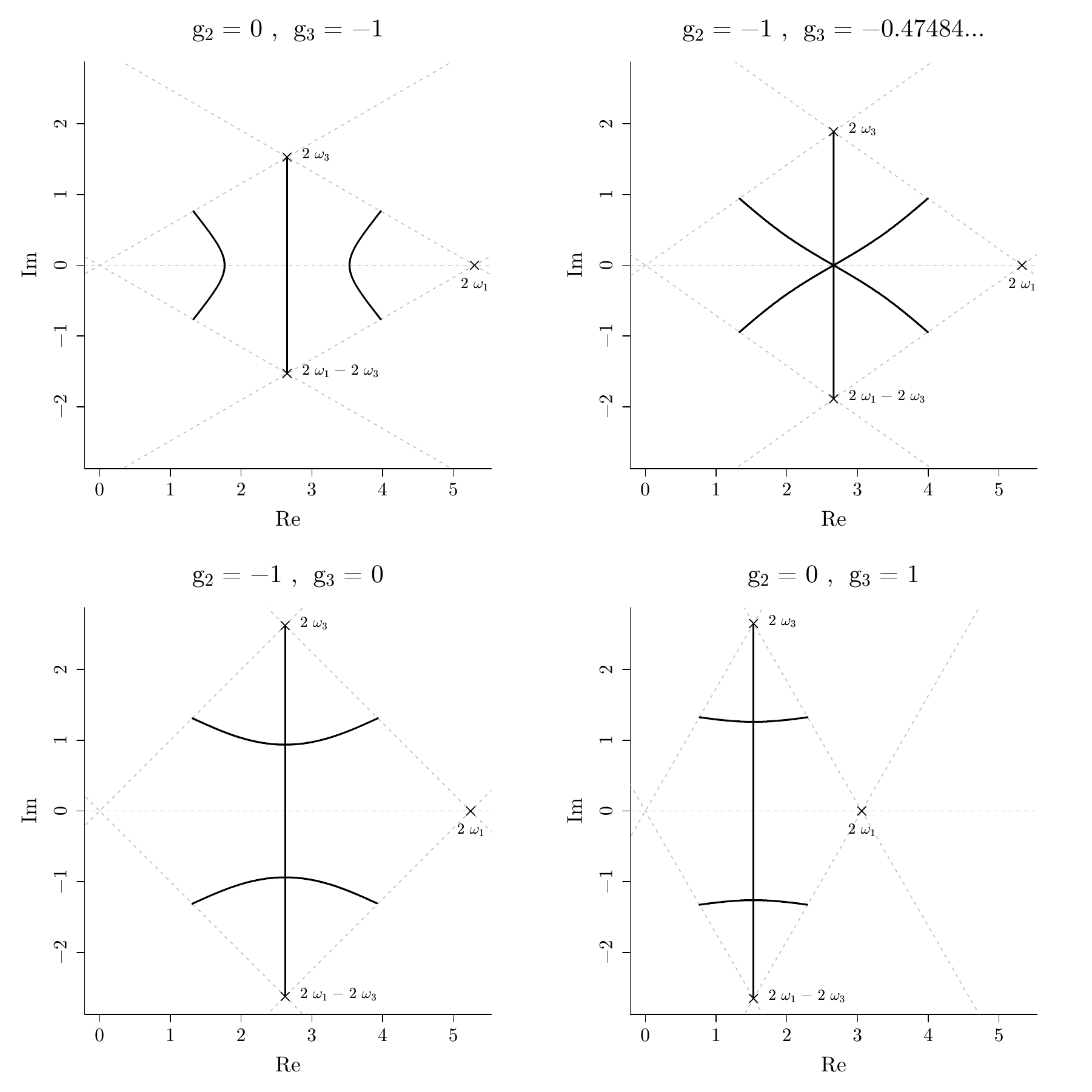
Figure 6: The set $\bar{Z}_{u}$ for rhombic period lattices ${\mathcal{L}}$, $m=1$ and $\omega=\omega_{1}$.

Proposition 3.9.

In the rhombic case (3.18) the spectrum of the complex Lamé operator (3.1) with $\omega=\omega_{1}$ is invariant under $\lambda\to\bar{\lambda}$, and the spectral arc extending to infinity coincides with $[-\omega_{1}^{2}e_{1},\infty)$. Moreover, all closed spectral gaps are located on the spectral arc extending to infinity.

Proof.

Recalling that the spectrum is given by

$$\lambda=-\omega_{1}^{2}\wp(k),\qquad k\in Z_{u},$$

invariance under complex conjugation follows immediately from

$$\zeta(\bar{k})=\overline{\zeta(k)},\qquad\wp(\bar{k})=\overline{\wp(k)}.$$

Combining these identities with $2\omega_{3}-\omega_{1}\in i(0,\infty)$, we see that

$$k=(2\omega_{3}-\omega_{1})s\in\bar{Z}_{u},\qquad-1\leq s\leq 1.$$

Since $\bar{\lambda}=\lambda$ for $k=(2\omega_{3}-\omega_{1})s$, $0<s\leq 1$, Proposition 3.5 and $2\omega_{3}-\omega_{1}=\omega_{1}$ $(\operatorname{mod}~{}\mathcal{L})$ imply that $[-\omega_{1}^{2}e_{1},\infty)$ coincides with the spectral arc extending to infinity.

Observing that the spectrum in the pseudo-lemniscatic case $\omega_{1}\in(0,\infty)$ and $2\omega_{3}=(1+i)\omega_{1}$ (see the lower left plot in Fig. 2) is identical to that in the lemniscatic case, the proof of Theorem 3.6 is readily adapted to the rhombic case. ∎

Now let us study the corresponding non-degeneracy conditions

$$\eta_{1}+\omega_{1}e_{j}\neq 0,\qquad j=1,2,3.$$

Theorem 3.10.

In the rhombic case with $m=1$ the non-degeneracy conditions are violated for exactly one exceptional curve $\mathcal{E}_{*}$ uniquely determined by the condition

$$\eta_{1}+\omega_{1}e_{1}=0.$$ (3.19)

The corresponding spectrum has a tripod structure with three simple analytic arcs joined at $2\pi/3$ angles. The same curve is the bifurcation point for the non-singularity condition (3.9), separating the cases with intersecting and non-intersecting spectral arcs.

Proof.

First of all, since both $\eta_{1}$ and $\omega_{1}$ are real the degeneracy condition $\eta_{1}+\omega_{1}e_{j}=0$ implies that the corresponding $e_{j}$ must be real too, so $e_{j}=e_{1}$.

Recall now that $2\omega$ and $2\eta$ are the complete first and second kind elliptic integrals, which can be also written as integrals

$$2\omega=\oint_{\gamma}\frac{{\rm d}E}{\sqrt{4(E-e_{1})(E-e_{2})(E-e_{3})}},\qquad 2\eta=-\oint_{\gamma}\frac{E{\rm d}E}{\sqrt{4(E-e_{1})(E-e_{2})(E-e_{3})}}$$

over the corresponding closed contour $\gamma$ in the complex domain. In our case the contour $\gamma$ is going around $e_{1}$ and $\infty$, or, equivalently, around the two complex conjugated roots $e_{2}$ and $e_{3}$. The degeneracy condition (3.19) can be rewritten then as

$$\oint_{\gamma}\frac{(E-e_{1}){\rm d}E}{\sqrt{4(E-e_{1})(E-e_{2})(E-e_{3})}}=0,$$ (3.20)

which also appeared in [1].

We have to show that there exists exactly one such curve. It would be convenient to use the parametrisation of the rhombic curves by fixing $e_{2}=i$, $e_{3}=-i$ and $e_{1}=t\in\mathbb{R}$ (Weierstrass’s restriction $e_{1}+e_{2}+e_{3}=0$ is violated, but this is not essential). We have to show that $\Phi(t)=0$ has the only real solution $t=t_{*}$, where

$$\Phi(t):=\oint_{\gamma}\frac{(E-t){\rm d}E}{\sqrt{4(E-t)(E-i)(E+i)}}=\oint_{\gamma}\sqrt{\frac{E-t}{4(E^{2}+1)}}{\rm d}E.$$

Its derivative has the form

$$\frac{{\rm d}}{{\rm d}t}\Phi(t)=-\frac{1}{2}\oint_{\gamma}\frac{{\rm d}E}{\sqrt{4(E^{2}+1)(E-t)}},$$

which is clearly negative since the integrand is positive on the half-line $E\in(t,\infty)$. Thus $\Phi(t)$ is strictly monotonically decreasing on the whole real line, which proves the uniqueness of the solution $t_{*}$. To show the existence it is enough to check that $\Phi(-2)>0$ and $\Phi(2)<0$ (e.g., numerically).

Numerical calculations give the value of the $j$-invariant

$$j=1728\frac{g_{2}^{3}}{g_{2}^{3}-27g_{3}^{2}}$$

of the corresponding elliptic curve to be $j_{*}\approx 243.797$. One can see the corresponding period lattice $\mathcal{L}_{*}$ in the top right corner of Fig. 6.

The tripod structure of the corresponding spectrum follows from a very general result by Batchenko and Gesztesy [1, Theorem 1.1(v)]. Its image is shown in the top right corner of Fig. 2.

The equal angles at the intersection point, which is also a general result due to Batchenko and Gesztesy [1], is readily verified. Indeed, $\lambda$ is contained in the spectrum if and only if $\tau(\lambda)=\mathrm{tr}M(\lambda)\in[-2,2]\subset\mathbb{C}$, where $M(\lambda)$ is the monodromy matrix. Since $M(\lambda)$ depends analytically on $\lambda$, we have locally

$$\tau(\lambda)=a_{0}+(\lambda-\lambda_{0})^{k}+\cdots$$

for some $k\in\mathbb{N}$. If $a_{0}=\pm 2$, which corresponds to $\lambda_{0}$ being an end point of the spectral arc, we have an $k$-pod with angles $2\pi/k$, see e.g. tripod in Fig. 2. If $a_{0}\in(-2,2)$, then we have $k$ arcs intersecting at $\lambda_{0}$ with angles between neighbouring arcs being $\pi/k$, see, e.g., the $k=2$ cases in the bottom two plots in Fig. 2.

To study the non-singularity condition recall that the critical points $k^{*}$ of the function $u(k)$ are given by $\eta+\omega\wp(k^{*})=0$. This means that the corresponding value of $\lambda(k^{*})=-\omega^{2}\wp(k^{*})=\eta\omega$ is real in this case. The non-singularity condition corresponds to the case when this value does not belong to the spectrum. Since the real part of the spectrum is $(-\omega^{2}e_{1},\infty)$ it holds iff $\eta\omega<-\omega^{2}e_{1}$, which is equivalent to $\eta+\omega e_{1}<0$. ∎

4 A qualitative analysis of the $\boldsymbol{m=2}$ case

Consider now briefly what happens in the case $m=2$. The spectral curve of the corresponding Lamé operator

$$L=-\frac{{\rm d}^{2}}{{\rm d}x^{2}}+6\omega^{2}\wp(\omega x+z_{0}),$$ (4.1)

has the form

$$w^{2}=\big{(}z^{2}-3g_{2}\big{)}\big{(}4z^{3}-9g_{2}z-27g_{3}\big{)}.$$ (4.2)

We restrict the attention to the rhombic case when $\Delta=g_{2}^{3}-27g_{3}^{2}<0$ and $\omega=\omega_{1}$. Setting $g_{3}=1$, this corresponds to $g_{2}\in(-\infty,3)$.

For $g_{2}\in(0,3)$, the roots of the first factor in the right-hand side of (4.2)

$$z^{2}-3g_{2}=0$$

yield two real endpoints $\lambda=\omega^{2}z=\pm\omega^{2}\sqrt{3g_{2}}$, whereas the second factor

$$4z^{3}-9g_{2}z-27g_{3}=0$$

gives one real positive endpoint as well as a complex conjugate pair of endpoints.

Hence we expect that for $g_{2}\in(0,3)$ the spectrum of (4.1) consists of two real intervals, one of which extends to infinity, and one arc connecting the two complex endpoints. Moreover, as $g_{2}\to 0$, the finite interval collapses to a double point. We can see this in the first two plots in Fig. 7, produced numerically using the software R. Note that in the special case $g_{2}=0$, the spectrum consists of only two arcs.

For $g_{2}\in(-\infty,0)$, the first factor yields two purely imaginary endpoints $\lambda=\pm i\omega^{2}\sqrt{-3g_{2}}$, which suggests a spectrum consisting of two arcs each connecting two endpoints in the upper- and lower- half-plane, respectively, and a real interval extending to infinity (see the last plot in Fig. 7).

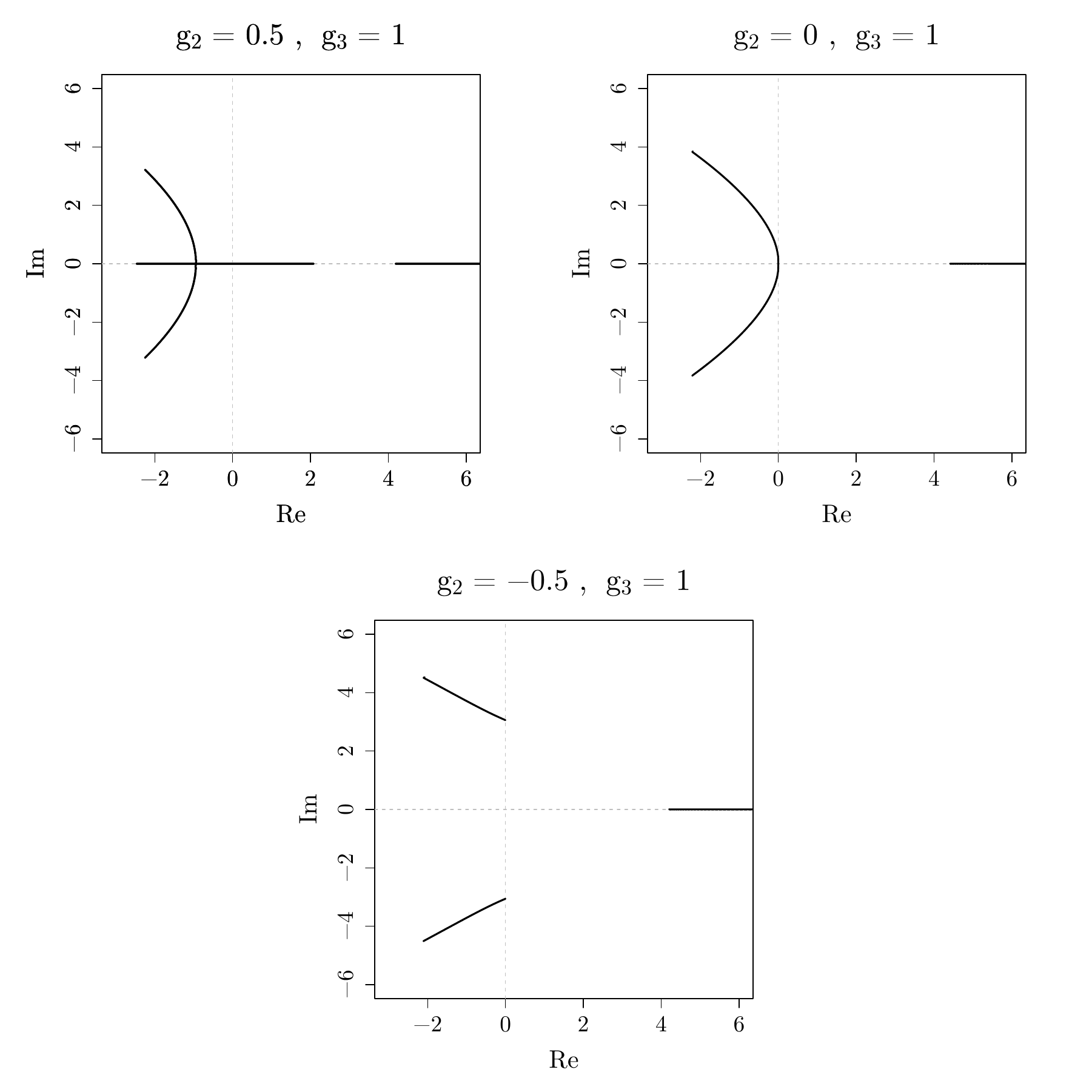
Figure 7: Different types of spectra of the complex Lamé operator (4.1) with $g_{3}=1$, depending on the sign of $g_{2}\in(-\infty,3)$.

5 Concluding remarks

The spectral theory of non-self-adjoint operators, in particular Schrödinger operators with complex potentials, has attracted significant attention in the last two decades, see, e.g., [4, 5, 30]. Nevertheless, it is fair to say that it is still a far less complete theory than in the self-adjoint case. In particular, we feel there is a need for more examples, which can be studied explicitly (like the complex harmonic oscillator in [4]).

In our paper we used the example of the classical Lamé equation, whose general solution was found by Hermite in the 19th century. This example was already briefly discussed in a much wider framework in [1, 9], but we believe that the complete picture was missing even in the simplest $m=1$ case. We used Hermite’s explicit formulae and Morse theory ideas to study the structure of the spectrum of complex Lamé operators for two different types of real elliptic curves with rectangular and rhombic lattices. The rigorous analysis of higher $m$ cases seems to be difficult since the explicit formulae quickly become quite complicated as $m$ grows, see [2, 11, 12].

A closely related interesting problem is to study the spectrum of the difference version of the Lamé operator

$$\mathcal{L}=\frac{\theta_{1}(x-m\eta)}{\theta_{1}(x)}T^{\eta}+\frac{\theta_{1}(x+m\eta)}{\theta_{1}(x)}T^{-\eta},$$

where $T^{\eta}$ is the shift operator defined by $T^{\eta}\psi(x)=\psi(x+\eta)$, and $\theta_{1}(x,\tau)$ is the odd Jacobi theta function (see [32] and references therein). When $\eta=\frac{p}{q}$ is rational we have an operator with periodic coefficients, in general complex. We expect that the geometry of the corresponding spectrum (in particular, the band structure in the real case) depends on the arithmetic of $p$ and $q$.

Acknowledgements

We are grateful to Jenya Ferapontov, John Gibbons and Anton Zabrodin for very useful and encouraging discussions, and especially to Boris Dubrovin, who many years ago asked one of us (APV) about the position of open gaps in the spectra of Lamé operators. We would like to thank Professor Gesztesy for his interest in our work and for pointing out further relevant references, including [1] and [9]. The work of WAH was partially supported by the Department of Mathematical Sciences at Loughborough University as part of his PhD studies.

References

• [1] Batchenko V., Gesztesy F., On the spectrum of Schrödinger operators with quasi-periodic algebro-geometric KdV potentials, J. Anal. Math. 95 (2005), 333–387, math.SP/0312200.
• [2] Belokolos E.D., Enolskii V.Z., Reduction of Abelian functions and algebraically integrable systems. II, J. Math. Sci. 108 (2002), 295–374.
• [3] Birnir B., Complex Hill’s equation and the complex periodic Korteweg–de Vries equations, Comm. Pure Appl. Math. 39 (1986), 1–49.
• [4] Davies E.B., Pseudo-spectra, the harmonic oscillator and complex resonances, R. Soc. Lond. Proc. Ser. A Math. Phys. Eng. Sci. 455 (1999), 585–599.
• [5] Davies E.B., Non-self-adjoint differential operators, Bull. London Math. Soc. 34 (2002), 513–532.
• [6] Drazin P.G., Johnson R.S., Solitons: an introduction, Cambridge Texts in Applied Mathematics, Cambridge University Press, Cambridge, 1989.
• [7] Dubrovin B.A., Matveev V.B., Novikov S.P., Non-linear equations of Korteweg–de Vries type, finite-zone linear operators, and Abelian varieties, Russ. Math. Surv. 31 (1976), no. 1, 59–146.
• [8] Erdélyi A., On Lamé functions, Philos. Mag. 31 (1941), 123–130.
• [9] Gesztesy F., Weikard R., Floquet theory revisited, in Differential Equations and Mathematical Physics (Birmingham, AL, 1994), Int. Press, Boston, MA, 1995, 67–84.
• [10] Gesztesy F., Weikard R., Picard potentials and Hill’s equation on a torus, Acta Math. 176 (1996), 73–107.
• [11] Grosset M.P., Veselov A.P., Elliptic Faulhaber polynomials and Lamé densities of states, Int. Math. Res. Not. 2006 (2006), 62120, 31 pages, math-ph/0508066.
• [12] Grosset M.P., Veselov A.P., Lamé equation, quantum Euler top and elliptic Bernoulli polynomials, Proc. Edinb. Math. Soc. 51 (2008), 635–650, math-ph/0508068.
• [13] Hermite C., Sur quelques applications des fonctions elliptique, C. R. Acad. Sci. Paris 85 (1877), 689–695, 728–732, 821–826.
• [14] Ince E.L., Further investigations into the periodic Lamé functions, Proc. Roy. Soc. Edinburgh 60 (1940), 83–99.
• [15] Kramers H.A., Ittmann G.P., Zur Quantelung des asymmetrischen Kreisels, Z. Phys. 53 (1929), 553–565.
• [16] Kramers H.A., Ittmann G.P., Zur Quantelung des asymmetrischen Kreisels. II, Z. Phys. 58 (1929), 217–231.
• [17] Lamé G., Sur les surfaces isothermes dans les corps homogènes en équilibre de température, J. Math. Pures Appl. 2 (1837), 147–188.
• [18] Lax P.D., Periodic solutions of the KdV equation, Comm. Pure Appl. Math. 28 (1975), 141–188.
• [19] Magnus W., Winkler S., Hill’s equation, Interscience Tracts in Pure and Applied Mathematics, Vol. 20, Interscience Publishers John Wiley & Sons  New York – London – Sydney, 1966.
• [20] Milnor J., Morse theory, Annals of Mathematics Studies, Vol. 51, Princeton University Press, Princeton, N.J., 1963.
• [21] Novikov S.P., The periodic problem for the Korteweg–de vries equation, Funct. Anal. Appl. 8 (1974), 236–246.
• [22] Olver F.W.J., Lozier D.W., Boisvert R.F., Clark C.W. (Editors), NIST handbook of mathematical functions, U.S. Department of Commerce National Institute of Standards and Technology, Washington, DC, Cambridge University Press, Cambridge, 2010, available at http://dlmf.nist.gov.
• [23] Pastur L.A., Tkachenko V.A., On the geometry of the spectrum of the one-dimensional Schrödinger operator with periodic complex-valued potential, Math. Notes 50 (1991), 1045–1050.
• [24] Reed M., Simon B., Methods of modern mathematical physics. IV. Analysis of operators, Academic Press, New York – London, 1978.
• [25] Reed M., Simon B., Methods of modern mathematical physics. I. Functional analysis, 2nd ed., Academic Press, Inc., New York, 1980.
• [26] Rofe-Beketov F.S., On the spectrum of non-selfadjoint differential operators with periodic coefficients, Soviet Math. Dokl. 4 (1963), 1563–1566.
• [27] Szegő G., Orthogonal polynomials, American Mathematical Society Colloquium Publications, Vol. 23, Amer. Math. Soc., Providence, R.I., 1959.
• [28] Takemura K., Analytic continuation of eigenvalues of the Lamé operator, J. Differential Equations 228 (2006), 1–16, math.CA/0311307.
• [29] Tkachenko V.A., Spectral analysis of the one-dimensional Schrödinger operator with periodic complex-valued potential, Soviet Math. Dokl. 5 (1964), 413–415.
• [30] Weikard R., On Hill’s equation with a singular complex-valued potential, Proc. London Math. Soc. 76 (1998), 603–633.
• [31] Whittaker E.T., Watson G.N., A course of modern analysis, Cambridge Mathematical Library, Cambridge University Press, Cambridge, 1996.
• [32] Zabrodin A., On the spectral curve of the difference Lamé operator, Int. Math. Res. Not. 1999 (1999), 589–614, math.QA/9812161.
\LastPageEnding