Gauge freedom in observables and Landsberg’s nonadiabatic geometric phase:
Pumping spectroscopy of interacting open quantum systems

Abstract

We set up a general density-operator approach to geometric steady-state pumping through slowly driven open quantum systems. This approach applies to strongly interacting systems that are weakly coupled to multiple reservoirs at high temperature, illustrated by an Anderson quantum dot. Pumping gives rise to a nonadiabatic geometric phase that can be described by a framework originally developed for classical dissipative systems by Landsberg. This geometric phase is accumulated by the transported observable (charge, spin, energy) and not by the quantum state. It thus differs radically from the adiabatic Berry-Simon phase, even when generalizing it to mixed states, following Sarandy and Lidar.

As a key feature, our geometric formulation of pumping stays close to a direct physical intuition (i) by tying gauge transformations to calibration of the meter registering the transported observable and (ii) by deriving a geometric connection from a driving-frequency expansion of the current. Furthermore, our approach provides a systematic and efficient way to compute the geometric pumping of various observables, including charge, spin, energy and heat. These insights seem to be generalizable beyond the present paper’s working assumptions (e.g., Born-Markov limit) to more general open-system evolutions involving memory and strong-coupling effects due to low temperature reservoirs as well.

Our geometric curvature formula reveals a general experimental scheme for performing geometric transport spectroscopy that enhances standard nonlinear spectroscopies based on measurements for static parameters. We indicate measurement strategies for separating the useful geometric pumping contribution to transport from nongeometric effects.

A large part of the paper is devoted to an explicit comparison with the Sinitsyn-Nemenmann full-counting statistics (FCS) approach to geometric pumping, restricting attention to the first moments of the pumped observable. Covering all key aspects, gauge freedom, pumping connection, curvature, and gap condition, we argue that our approach is physically more transparent and, importantly, simpler for practical calculations. In particular, this comparison allows us to clarify how in the FCS approach an “adiabatic” approximation leads to a manifestly nonadiabatic result involving a finite retardation time of the response to parameter driving.

I Introduction

I.1 Geometric effects in open quantum systems

Currently there is a heightened interest in geometric and topological properties of open quantum systems where finite temperature, dissipation, and non-equilibrium transport play a key role. For closed quantum systems topological properties are generally appreciated for their robustness against perturbations, assuming these perturbations keep the system closed. This robustness, for example, underlies the successful topological classification of phases of closed quantum systems Altland and Zirnbauer (1997); Read and Green (2000); Snyder and Toberer (2008); Nayak et al. (2008a); Kitaev (2009); Ryu et al. (2010); Hasan and Kane (2010); Qi and Zhang (2011); Budich et al. (2015); Chiu et al. (2016); Kennedy and Zirnbauer (2016). It is a pressing question as to how this scheme is affected when one opens up the system, allowing for finite temperature, dissipation, and nonequilibrium Diehl et al. (2011); Bardyn et al. (2013); Iemini et al. (2016). To address this issue, recently topological numbers for dissipative systems have been discussed Huang and Arovas (2014); Viyuela et al. (2015); Budich et al. (2015); Budich and Diehl (2015) starting from the Uhlmann connection for mixed quantum states Uhlmann (1986). One may also utilize topological robustness for controlling quantum systems. For example, in the area of quantum information processing this is exploited in geometric quantum computing Zanardi and Rasetti (1999) and in topological error correction Dennis et al. (2002); Nayak et al. (2008b). Ultimately, topological properties stand in the foreground because of their superior robustness as compared to geometric properties. However, as for classical mechanics Marsden et al. (1990); Marsden and Ostrowski (1998); Cendra et al. (2001); Bloch (2003); Andersson (2003a), also for quantum systems a deep understanding of the underlying geometric properties is always a prerequisite for such control. One of the reasons why the geometric properties of open quantum systems are more complex than for closed systems is that they are described by mixed states rather than pure states Uhlmann (1986); Dabrowski and Grosse (1990); Sjöqvist et al. (2000); Zhou et al. (2003); Ericsson et al. (2003); Cohen (2003); Whitney and Gefen (2003); Whitney et al. (2005); Chu and Telnov (2004); Tong et al. (2004); Chaturvedi et al. (2004); Sarandy and Lidar (2005, 2006); Fujikawa (2007); Sinitsyn and Nemenman (2007a); Goto and Ichimura (2007); Whitney (2010); Avron et al. (2012a). However, as this paper will emphasize, this is not the only important difference. There are also important geometric properties associated with observables Avron et al. (2012a), including nonsystem observables Sinitsyn (2009) defined (partly) on the system’s environment and their transport currents.

Indeed, geometric effects appear naturally in open quantum systems when considering pumping of some observable quantity, e.g., charge, which has been studied extensively in electronic systems. In the long-time limit the transport through a mesoscopic system exhibits steady-state pumping when its external parameters are periodically modulated in time Grifoni and Hänggi (1998). For example, in highly-tunable quantum-dot systems one can drive local system properties via electrical gates, modulate the coupling to external reservoirsKaestner and Kashcheyevs (2015) by tunnel barriers, or vary the external electro-chemical potentials Brouwer (2001) or temperatures Watanabe and Hayakawa (2014). Such time-dependent control has been experimentally demonstrated even for atomic-scale junctions Boeuf et al. (2003) and is also of interest for realizing molecular motors Chernyak and Sinitsyn (2009); Napitu and Thijssen (2015).

When slowly driving an open quantum system, there are two effects to consider. First, one generically obtains a nonequilibrium current at every instant in time if there is an instantaneous (possibly time-dependent) bias applied, either electrochemical or thermal or both. This survives even in the adiabatic limit of vanishing driving frequency $\Omega$. The net transported observable after one cycle then generically contains an average over these instantaneous currents (“sum of snapshots”). Since this part of the current is invariant under inversion of the parameter driving, its effect can always be canceled out experimentally or extracted theoretically.

However, there is also the pumping current contribution which only derives from this time-dependent driving Büttiker et al. (1985); Brouwer (1998). Physically, this contribution clearly differs from the instantaneous one: it arises because the state of the open system cannot instantaneously follow the driving but lags behind. It derives from the time-average of the nonadiabatic part of the current that is linear in driving frequency $\Omega$. Nevertheless, this pumping effect is often referred to as “adiabatic pumping”  Brouwer (1998); Switkes et al. (1999); Splettstoesser et al. (2006); Sinitsyn and Nemenman (2007a) which we will emphatically avoid here. In this paper, we focus on this adiabatic-response pumping in open quantum systems which has the hallmark of a geometric quantityResta (2000); Xiao et al. (2010); Bohm et al. (2003); Marsden et al. (1990); Nakahara (2003) in its simplest meaning: the transported observable per cycle depends on the driving parameter curve alone and not on the driving frequency, in contrast to the nongeometric, instantaneous part. Pumping thus arises as an adiabatic response to drivingAvron et al. (2012a); Berry and Robbins (1993) (“lag”) and is inherently a (first-order) nonadiabatic geometric effect, in contrast to the more commonly considered geometric phases associated with adiabatic dynamics Berry (1984); Bohm et al. (2003); Sarandy and Lidar (2006).

One reason for studying the geometric nature of pumping lies in robust control of transport of quantities like charge, spin, or energy. For example, for applications to charge-current standardsPekola et al. (2013) the robustness of the geometric pumping with respect to frequency-fluctuations is relevant. Therefore, it is of practical importance to be able to separate clearly this frequency-independent pumped observable, responsible for “clocked” electron transfer Roche et al. (2013), from the driving-frequency-dependent nongeometric contribution. The present paper shows that a separate consideration of the geometric adiabatic-response part is also of theoretical importance for identifying the physical origin of the gauge freedom underlying pumping.

Further motivation is provided by the interest in topological pumping mentioned at the beginning: namely, topological pumping arises when geometric quantities depend only on the “type” of the driving cycle (homotopy class). For example, one characteristic is the number of windings of the parameter cycle around a “hole” in parameter space (similar to the Aharonov-Bohm effect). As long as this characteristic stays unchanged, the pumped quantity is even protected against continuous deformations of the geometric properties of the driving cycle.

In this work, we are particularly interested in identifying the geometric nature of the pumping contribution in systems where strong interactions play a role. This is largely motivated by experiments on quantum dot systems  in which one can exploit strong Coulomb interactions to gain control over a single electron as already shown in early experiments on pumping Pothier et al. (1992). More recently, accurately clocked sources of single charges Fève et al. (2007); Roche et al. (2013); Pekola et al. (2013) or spins Xing et al. (2014); Dittmann et al. (2016) have been implemented. This illustrates the high degree of control over single electrons in a quantum-dot system in time.

The final point of interest, going beyond the aspects of robustness and control, is the use of pumping as a “spectroscopic” tool. In this paper, we discuss how pumping effects can shed light on properties of an open quantum system that remain hidden when considering only non-driven, stationary transport. This has use as an experimental tool, since one can infer, for example, the tunnel-coupling asymmetry and the spin-degeneracy of a quantum dot just by using the qualitative features of an interaction-induced charge pumping Reckermann et al. (2010); Calvo et al. (2012); Riwar et al. (2013) effect. However, it may also function as a theoretical tool similar to the usual linear response to a perturbation: in models that are theoretically hard to analyze, physical characteristics that are not revealed by stationary properties (e.g., due to renormalization effects) may well appear in an adiabatic-response calculation of pumping effects Splettstoesser et al. (2006).

Table 1: Comparison of geometric density-operator approaches relevant to this paper.

Approach	Prior works	Present work
(I) Adiabatic state	Adiabatic mixed-state geometric phase Sarandy and Lidar (2005, 2006)	Zero geometric phase for adiabatic steady-state [Sec. III.1]
evolution (ASE)	Mixed-state adiabatic-response correction Sarandy and Lidar (2005, 2006)	Zero geometric phase for nonadiabatic state [Sec. III.1]
	Gauge freedom related to eigenvector rescaling Sarandy and Lidar (2005, 2006)	Restriction of gauge freedom by normalization and hermiticity [Sec. III.1]
(II) Full counting	Geometric part of generating function Sinitsyn and Nemenman (2007a); Sinitsyn (2009); Chernyak et al. (2012a, b); Chernyak and Sinitsyn (2010); Ivanov and Abanov (2010)	Restriction of gauge freedom by real-valuedness observable [Sec. V.3.3]
statistics (FCS)	All moments have geometric part Sinitsyn and Nemenman (2007a); Sinitsyn (2009)	Clarification of “adiabaticity” in FCS [Sec. V.3.4]]
		Conditions for applicability same as in AR [Sec. V.3.4]]
(III) Adiabatic	Adiabatic-response of unique stationary state Avron et al. (2012a)	Adiabatic iteration for Born-Markov open system [Sec. III.1,Appendix H]
response (AR)	Geometric pumping of system observable Avron et al. (2012a)	Physical picture of gauge freedom in observable [Sec. III.2]
		Gauge freedom of current memory kernels [Sec. III.2]
		Geometric pumping of nonsystem observables [Sec. III.3]

Table 2: Cross-links between geometric density-operator approaches discussed in this paper.

Approaches	Cross links in present work
ASE $\leftrightarrow$ FCS	FCS is equivalent to the ASE approach
	with $\chi$ dependence
ASE $\leftrightarrow$ AR	Nonadiabatic correction to ASE [Eq. (23) of LABEL:Sarandy05]
	agrees with AR result $\rho^{\text{a}}$ [Eq. (43b)]
	but contributes zero in unique steady-state [Sec. III.1]
	AR Geometric phase instead in observable.
AR $\leftrightarrow$ FCS	Nonadiabatic Landsberg phase [Sec. V.3.4]
	equal to $\chi$-linear part of FCS-phaseNakajima et al. (2015)

Before we can formulate the open questions that our key results address, we need to outline a number of existing theoretical approaches to pumping. This also serves to keep the paper self-contained and makes it more accessible to readers with interest in either geometrical effects or open quantum systems or both. This seems furthermore warranted since a number of quite different approaches, designed to deal with different problems, have been put forward. We also point out a number of useful relations between cited references that have received little attention so far. A guide to our comparison of the geometric aspects of these approaches and different aspects put forward in this work is given in Table 1 and 2.

I.2 Geometric density operator approaches

For open systems without interactions (beyond the mean-field level), Brouwer’s framework Büttiker et al. (1993, 1994); Brouwer (1998) for pumping based on the Buttiker-Thomas-Pretre scattering theory for time-dependent setups is by now standard. Within this approach, the geometric nature of charge pumping is associated with unitary transformations of the scattering matrices Altshuler and Glazman (1999); Zhou et al. (2003). This has played an important role, for example, in recent theoretical work on current-induced forces in nanoscale systems Dundas et al. (2009); Bode et al. (2011); Thomas et al. (2012); Todorov et al. (2014); Lü et al. (2015) and nanoscale motors Hänggi and Marchesoni (2009); Seldenthuis et al. (2010); Bustos-Marún et al. (2013); Napitu and Thijssen (2015); Arrachea and von Oppen (2016).

However, when strong interactions become important one needs a different approach, even though Brouwer-type formulas emerge also in this case Calvo et al. (2012) (see Appendix F). Whereas Green’s function approaches to pumping have been put forward Splettstoesser et al. (2005); Sela and Oreg (2006); Fioretto and Silva (2008), there is a well-established approach to strongly interacting systems based on the reduced density operator description. However, within this approach the situation is less univocal regarding the geometric nature of pumping. This is a primary topic of this paper. Several geometric frameworks have been formulated based on the reduced density operator, including contexts unrelated to pumping. We will tie together three of these formulations, found in Refs. Sarandy and Lidar, 2005, Sarandy and Lidar, 2006 and LABEL:Avron12, and Refs. Sinitsyn and Nemenman, 2007a, Sinitsyn, 2009, Nakajima et al., 2015, respectively. Before we outline the key results of our paper, we sketch these three geometric approaches, taking note of many other density-operator based works Uhlmann (1986); Dabrowski and Grosse (1990); Sjöqvist et al. (2000); Zhou et al. (2003); Ericsson et al. (2003); Cohen (2003); Whitney and Gefen (2003); Whitney et al. (2005); Chu and Telnov (2004); Tong et al. (2004); Chaturvedi et al. (2004); Fujikawa (2007); Goto and Ichimura (2007); Whitney (2010).

(i) Adiabatic state-evolution (ASE) approach. A perhaps intuitive, but wrong expectation is that the geometric nature of pumping in open systems arises from the dynamics of the reduced quantum state. However, in the following [cf. also LABEL:Pluecker16b] it is still important to consider such geometric phases. The geometric nature of this adiabatic mixed-state evolution has been worked out by Sarandy and LidarSarandy and Lidar (2005, 2006). This closely follows the analogy to the adiabatic Berry-Simon phase for adiabatic evolution of a pure state of a closed quantum system. In the ASE approach the mixed-state density operator $\rho(t)$ is considered as a ket vector ${|{\rho(t)})}$ in Liouville (or Hilbert-Schmidt) space evolving according to a time-local master equation

$$\frac{d}{dt}{|{\rho(t)})}=W[{\mathbf{R}}(t)]\,{|{\rho(t)})}.$$ (1)

Here, the kernel $W[{\mathbf{R}}(t)]$ takes over the role of the evolution generator played by the Hamiltonian $H[{\mathbf{R}}(t)]$ in the Berry-Simon case based on the Schrödinger equation $\tfrac{d}{dt}|\psi(t)\rangle=-iH[{\mathbf{R}}(t)]\,|\psi(t)\rangle$ for natural units setting $\hbar=\text{k}_{\text{B}}=\text{e}=1$. The time dependence enters entirely through the instantaneous values of the driving parameters ${\mathbf{R}}(t)$. Similar to the Berry-Simon approach, in the ASE approach one expands the solution of the master equation in the eigenvectors ${|{v_{n}})}$ to eigenvalues $\lambda_{n}$ of the kernel $W$, all with parametric time-dependence. A gauge freedom emerges from the nonuniqueness of the normalization of these eigenvectors, but in contrast to the Berry-Simon case, these changes in the normalization are nonzero complex numbers (nonunitary, noncompact gauge group), rather than phase factors (unitary, compact). For slow driving, the solution of the master equation (1) follows (a sum of) these eigenvectors adiabatically resulting in dynamical and geometric phases. Several points discussed in this paper can be understood as a formal application of this generalization of the Berry-Simon phase. However, the ASE approach does not deal with steady-state pumping and the ASE phase essentially differs from the simple geometric pumping phase that we work out here: in our contexts the ASE phase for the steady state is identically zero, even when accounting for the first nonadiabatic correction (adiabatic-response) to the state. This quenching of the Berry-Simon type phase of mixed states forms the starting point for the considerations of geometric steady-state pumping.

(ii) Full-counting statistics (FCS) approach to pumping. Within the density operator framework, the geometric nature of pumping of observables was first clarified when Sinitsyn and NemenmannSinitsyn and Nemenman (2007a) applied the well-established FCS approach to pumping (“stochastic pumping”), introduced in more detail in Sec. V. Interestingly, they found that pumping can be induced by interaction. In the FCS one uses an observable-specific generating function $Z^{\chi}$ depending on a “counting field” variable $\chi$ to obtain the statistics of a selected observable, i.e., all its moments and their dynamics. From this generating function the change of the first moment of a reservoir observable $X^{r}$ can be obtained as

$${\langle{{X}^{r}}\rangle}(t)-{\langle{{X}^{r}}\rangle}(0)=\partial_{i\chi}\left.Z^{\chi}(t)\right|_{\chi=0}.$$ (2)

The generating function is obtained from a “generating operator” $\rho^{\chi}$, which is the “adiabatic” solution of a master-type equation similar to Eq. (1) and exhibits a geometric phase similar to the one calculated in the ASE problem. This elegant and powerful approach has been applied to various pumping problems and is reviewed in LABEL:Sinitsyn09: applications range from molecular reactions Sinitsyn and Nemenman (2007a, b); Sinitsyn (2009), to heat transport through strongly anharmonic molecules Ren et al. (2010); Liu et al. (2013), and strongly interacting quantum dots Bagrets and Nazarov (2003); Utsumi (2007); Yuge et al. (2012); Yoshii and Hayakawa (2013); Nakajima et al. (2015). It was also used to demonstrate that thermodynamic vector potentials arise in slow but nonadiabatic transformations between non-equilibrium steady-states Yuge et al. (2013) accounting for geometric heat and excess entropy production. In a recent paper Nakajima et al. (2015), Nakajima et al. addressed a possible point of confusion in the FCS approach: how can an “adiabatic” approach include physically nonadiabatic pumping? In the last part of this paper we will further clarify this issue, extending their observations.

(iii) Adiabatic-response (AR) approach. Finally, Avron et al. studied Avron et al. (2012a) pumping in the density operator approach also starting from Eq. (1). Interestingly, they considered pumping for both unique and nonunique frozen-parameter stationary states. The core idea of AR is to first expand the master equation (1) in the driving frequency (smallest time scale) and solve for the density operator in zeroth ($\rho^{\text{i}}$) and linear order ($\rho^{\text{a}}$) in this frequency:

$$\rho(t)\approx\rho^{\text{i}}(t)+\rho^{\text{a}}(t)+...\;.$$ (3)

Importantly, the nonadiabatic part $\rho^{\text{a}}$ accounts for the “laggy” response and generates the pumping. However, they restricted their analysis, using a Kato formulation, to pumping of system observables (i.e., with current operators related to particle transfer between parts within the open subsystem) and considered only a single reservoir. For the case of a unique stationary state, the adiabatic-response pumping of system-observables calculated in LABEL:Avron12 was related to Berry-Robbins’ “geometric magnetism” Robbins and Berry (1992); Berry and Robbins (1993); Berry and Sinclair (1997); Cohen (2003) formulation of pumping. In this paper, we instead study nonsystem observables and their currents to multiple reservoirs, which is crucial for describing the transport through an open quantum system, enabling a geometric transport spectroscopy. This requires account of an additional evolution equation, namely, for the current $I_{X}^{r}$ of a nonsystem observable $X^{r}$ into reservoir $r$:

$$I_{X}^{r}=\mathsf{Tr}W_{\hat{I}_{X^{r}}}\rho(t).$$ (4)

This brings in an additional observable-specific memory-kernel $W_{\hat{I}_{X^{r}}}$ whose role in generating a geometric adiabatic-response has not been addressed so far.

I.3 Summary of results

The present paper was inspired by all three outlined approaches, but in particular by a discussion in LABEL:Avron12 of the nonuniqueness of currents in relation to their observables, reaching back to earlier works Bellissard (2002); Gebauer and Car (2004); Bodor and Diósi (2006); Salmilehto et al. (2012). Following up on an earlier remark in LABEL:Sinitsyn09 (p. 8) we combine this idea with Landsberg’s approach Landsberg (1992); Andersson (2003a, 2005) to dissipative systems with symmetriesKepler and Kagan (1991); Ning and Haken (1992). The key point is to consider the physical role of the meter registering the pumping signal in the reduced density-operator formalism. This results in an intuitive and clear physical picture that does not seem to have been worked out so far.

We outline the main steps and results of this paper:

(1) Landsberg geometric phase for pumping. In pumping a local gauge freedom emerges in the relation between a measurable pumped observable and its associated current operator [Eq. (59)]. This is encoded in the simple adiabatic-response equations for the mixed quantum state,

$$0=W\rho^{\text{i}},\qquad\frac{d}{dt}\rho^{\text{i}}=W\rho^{\text{a}}$$ (5)

and an “enslaved” equation for the current for a nonsystem observable:

$$\frac{d}{dt}{\langle{\hat{X}^{r}_{g}}\rangle}=\mathsf{Tr}\,W_{\hat{I}_{X^{r}_{g}}}\left(\rho^{\text{i}}+\rho^{\text{a}}\right).$$ (6)

Here $W$ and $W_{\hat{I}_{X^{r}_{g}}}$ have only parametric time dependence. Crucially, this observable $\hat{X}^{r}_{g}(t)\coloneqq\hat{X}^{r}+g[{\mathbf{R}}(t)]\mathbbm{1}$ includes all possible parametrically time-dependent gauges $g$ relative to the “bare” time-constant observable $\hat{X}^{r}$. Physically this gauge freedom corresponds to a calibration of the meter scale. In the current kernel a gauge transformation $g\to g+f$, a recalibration, leads to

$$W_{\hat{I}_{X^{r}_{g}}}\to W_{\hat{I}_{X^{r}_{g+f}}}=W_{\hat{I}_{X^{r}_{g}}}+{\mathbf{\nabla_{R}}}f,$$ (7)

requiring an extension of the Heisenberg equation of motion [Eq. (41)] to observables outside the open system. This makes the pumping contribution of the transported observable an instance of the geometric phase first considered by Landsberg

$$\Delta X^{r,\text{a}}=\oint_{C}d{\mathbf{R}}A_{X^{r}_{g}}[{\mathbf{R}}],$$ (8)

with the Landsberg connection (gauge potential) [Eq. (73)]:

$$A_{X^{r}_{g}}={({\mathds{1}}|}W_{\hat{I}_{X^{r}}}\frac{1}{W}{|{{\mathbf{\nabla_{R}}}\rho^{\text{i}}})}+{\mathbf{\nabla_{R}}}g,$$ (9)

where the pseudo inverse $1/W$ is defined on the nonzero eigenspaces of $W$.

(2) Pumping determines a geometric effect. Geometrically, the observable (not the quantum-state) plays the role of a fiber (group) coordinate in a (principal) fiber bundle over the space of driving parameters with a tangible physical meaning. The Landsberg geometric connection on this space is essentially the adiabatic-response part of the total current $I_{X^{r}_{g}}=I^{\text{i}}_{X^{r}_{g}}+I^{\text{a}}_{X^{r}_{g}}$ of a gauge-dependent observable. The geometric “horizontal lift” defined by this connection corresponds to maintaining the physical pumping current $I_{X^{r}_{g}}^{\text{a}}$ to be zero at each time instant by continuously adjusting the scale of the meter. The geometric-phase “jump,” the holonomy of a horizontal lift curve, corresponds physically to the resulting cumulative adjustment of the meter’s scale over a driving period: the pumped observable per period.

(3) Conditions for nonzero pumping curvature. The generic presence of gauge freedom implies that one can expect a geometric pumping contribution unless the connection $A_{X^{r}_{g}}$ is integrable for some special reason. The gauge-invariant curvature (gauge field)

$$B_{X^{r}}={({\mathds{1}}|}\Big{(}{\mathbf{\nabla_{R}}}W_{\hat{I}_{X^{r}}}\frac{1}{W}\Big{)}\times\Big{(}{\mathbf{\nabla_{R}}}{|{\rho^{\text{i}}})}\Big{)}$$ (10)

measuring this nonintegrability is just the pumped observable per unit area of the driving parameter space. This quantity is sensitive to crossings of lines in the parameter space where the open system is in resonance with the reservoirs. This enables a geometric spectroscopy of open quantum systems. Importantly, this formula also applies if there are no strict conservation laws, which is relevant, e.g., for spin- and heat transport. It can however be easily simplified if such laws are present. The application of our pumping formula to the explicit example of a single level Anderson quantum dot illustrates this spectroscopy, showing that for a variety of driving protocols, interaction is required to obtain a nonzero geometric pumping phase.

(4) Connections of different approaches. We find that the three approaches (ASE, AR, FCS) outlined in the previous section, are intimately related as summarized in Table 2. Our main line of comparison involves our AR approach with the FCS approach. We show that when the FCS is applied to the first moment of pumping, as done in many works, it is term-by-term equivalent to our much simpler AR approach on all levels (pumping formulas, gauge freedom, connection, curvature, and their limits of applicability). We show that the FCS not only unnecessarily complicates practical calculations, but is also less clear regarding the physical meaning of the geometric nature of pumping due to its “mixing” of effects of the quantum state and the observable [see discussion after Eq. (142)].

This comparison allows us to resolve the important issue regarding the “adiabaticity” of the FCS going beyond the scope of LABEL:Nakajima15. Also, we show how within this physical nonadiabatic picture of the AR approach the geometric nature of pumping can be fully understood, independent of the FCS formulation, thereby avoiding the nontrivial issue of its “adiabaticity”. In our comparison, the ASE approach turns out to be very relevant time and again. We also connect our approach to the Kato formulation of the AR approach of LABEL:Avron12, shedding some new light on it.

I.4 Adiabatic-response real-time approach beyond the Markovian, weak-coupling limit

An important implication of our work is that Landsberg’s geometric framework is compatible with a more general AR approach to pumping Splettstoesser et al. (2006) applicable to non-Markovian, strongly-coupled open quantum systems: the gauge freedom we point out derives from entirely general arguments. Since this paper is written with this future extensionPluecker et al. in mind, it is important to briefly outline this more general AR approach.

This general adiabatic-response approach to pumping in slowly driven open systems Splettstoesser et al. (2006) is based on the exact time-nonlocal kinetic equation for the density operator,

$$\frac{d}{dt}\rho(t)=-i[H[{\mathbf{R}}(t)],\rho(t)]+\int_{-\infty}^{t}dt^{\prime}W(t,t^{\prime};\{{\mathbf{R}}(\tau)\})\rho(t^{\prime}),$$ (11)

here written for the time-dependent steady-state limit, i.e., switching on the system-reservoir coupling at $t_{0}=-\infty$ and starting from an initially factorizing system-reservoir state. This approach is close in spirit to the AR approach to pumping mentioned above under point (iii). However, it goes beyond these by incorporating the fact that the open-system evolution has a functional dependence on the entire driving-parameter history, indicated by the dependence on $\{{\mathbf{R}}(\tau)\}$ of the kernel $W$. This is accomplished by systematically accounting for processes of higher order in the coupling as well as the Laplace-frequency dependence of both the kernel and the density operator. From this point of view, the superoperator $W$ in Eq. (1) only accounts for the zero-frequency ($z=i0$) part of the Laplace-transform of $W(z;{\mathbf{R}}(t))$ of the kernel in Eq. (11) after freezing its parameters at the latest time $\tau=t$.

Expectation values of nonsystem observables $X^{r}$, e.g., reservoir observables or reservoir-system currents, are described by a similar time-nonlocal equation:

$$\langle\hat{X}^{r}(t)\rangle=\mathsf{Tr}\,\int_{-\infty}^{t}dt^{\prime}W_{\hat{X}^{r}}(t,t^{\prime};\{{\mathbf{R}}(\tau)\})\rho(t^{\prime}),$$ (12)

with an observable-specific memory-kernel $W_{\hat{X}^{r}}$ that in general needs to be calculated separately in addition to $W$ in Eq. (11). A key point of the paper is that this equation requires careful consideration in order to ensure explicit physical gauge covariance of the formalism.

For strongly interacting open systems at low temperature the time-nonlocal kernels required in Eqs. (11) and (12) can be systematically computed using the real-time diagrammatic technique König et al. (1995); Schoeller (2009). This provides a general framework for calculating kernels, including those required for noise Aghassi et al. (2006), correlation functions Schuricht and Schoeller (2009); Schmidt et al. (2010), and  for the full counting statistics Braggio et al. (2006). The flexibility of this approach is illustrated by the possibility of formulating a nonequilibrium renormalization group scheme for calculating $\rho(t)$ Schoeller (2009); Eckel et al. (2010); Pletyukhov et al. (2010); Andergassen et al. (2011); Pletyukhov and Schoeller (2012); Saptsov and Wegewijs (2012); Klochan et al. (2013). For example, this enabled a nonperturbative adiabatic-response analysis Kashuba et al. (2012) of interaction effects on the universal charge-relaxation resistance Mora and LeHur (2010); Hamamoto et al. (2010); Lee et al. (2011) for strong tunnel coupling and low temperature.

So far in this more general setting little attention has been paid to the geometric aspects of pumping. This paper addresses two questions relevant to this: First, where in the formalism does the gauge freedom responsible for geometric pumping arise? What is its concrete physical meaning? Second, the general AR approach to pumping is based on real-time memory-kernels for nonsystem observables [Eq. (12)]. The role of these kernels for the geometric nature of pumping has not been considered at all within the other AR formulations outlined under point (iii) above. What is this role?

These questions are intimately related and lead to the insight that observables, rather than mixed quantum states, accumulate a geometric phase that is responsible for steady-state pumping. To see this, it is necessary, but not sufficient, to account for generically time-dependent observables, even when interested in the expectation values of time-constant ones. This is the fundamental difference to the AR approaches listed under point (iii) and also turns out to provide the link to the FCS approach point (ii). Fortunately, this can already be addressed in the much simpler setting of Eq. (1) instead of the general density-operator approach based on Eq. (11). In this paper we thus start from this equation, i.e., the same kind of master equation as the approaches (i)-(iii) reviewed above, allowing a useful three-way comparison. The generalization starting from Eqs. (11) and (12) requires more care and will be discussed elsewhere Wegewijs et al. .

I.5 Outline

In summary, our aim is to set up a geometric framework for pumping through strongly interacting open systems that can deal with nonsystem observables, that is more direct than the FCS approach (when targeting only the first moment), and that is a more suitable starting point for generalization to evolutions more complicated than Eq. (1). The outline of the paper is as follows:

In Sec. II, we review how the kernels for the evolution of the state [Eqs. (1) and (5)] and for the observable expectation values [Eq. (6)] can be derived. We pay attention to issues related to inadvertent gauge fixing by the common procedure of normal-ordering expressions with respect to the reservoirs. The key formula is the Heisenberg equation (41) for the current superoperator after the reservoirs have been integrated out. At the end of this section, we formulate the guiding questions for the remainder of the paper.

In Sec. III, we then show that in the pumping problem a gauge freedom emerges that is related to the physical calibration of the meter registering the transport of a nonsystem observable (reservoir charge, spin, heat, etc.). The pumping problem precisely fits into the general geometric framework of Landsberg Landsberg (1992) for driven dissipative systems with a continuous (gauge) symmetry. The solution determines a geometric connection (gauge potential) on a simple fiber bundle of observables over the manifold of driving parameters. This connection is essentially the nonadiabatic current response and is closely related to a meter calibration.

In Sec. IV, we analyze the expression for the corresponding geometric curvature (gauge field), essentially the measurable pumped observable, and determine necessary conditions for a nonzero pumping effect. We explain how under quite general circumstances pumping can be used to perform a geometric spectroscopy of a weakly coupled open system.

Finally, in the extensive Sec. V we compare the Landsberg-AR approach in detail with the FCS approach, when applied only to the first moment of the pumped observable. Despite the quite different formulation, we show that this approach is equivalent to the simpler and more direct Landsberg-AR approach on all levels: gauge freedom, connection (gauge potential), geometric pumping formula for the curvature (gauge field), as well as the limits of applicability. Our formulation highlights the physical role of the meter and allows us to further clarify the puzzling fact noted in LABEL:Nakajima15 that the “adiabatic” FCS approach produces nonadiabatic contributions.

II Adiabatic-response approach
to pumping

II.1 Model, pumped observables
and steady-state pumping

The adiabatic-response approach to pumping that we describe in this section applies to very general open quantum systems. We consider a quantum system with a discrete energy spectrum coupled to multiple noninteracting reservoirs indexed by $r$. Whereas the reservoirs are assumed to be made up of either fermions or bosons, the system can be of mixed type as well. We allow for possibly strong nonequilibrium conditions due to nonlinear biasing of the reservoirs’ electrochemical potentials ($\mu^{r}\neq\mu^{r^{\prime}}$). Of central importance is that our findings also apply to a quantum system that is locally strongly interacting, in contrast to several existing pumping approaches Brouwer (1998); Büttiker et al. (1994); Zhou et al. (2003). For example, Coulomb interaction is crucial if one wants to describe driven transport through quantum-dot devices, such as semi-conductor heterostructures Vanević et al. (2016), but also molecules Napitu and Thijssen (2015) and single atoms Boeuf et al. (2003). However, the approach applies equally well to bosonic models of pumping in chemical reactions between strongly interacting molecules Sinitsyn and Nemenman (2007a) and heat pumping using anharmonic Ren et al. (2010); Liu et al. (2013) molecules.

The total system has the generic form of the Hamiltonian

$$H^{\text{tot}}(t)=H(t)+\sum_{r}H^{r}(t)+V(t),$$ (13)

with $H$ describing the system. $H^{\text{res}}(t):=\sum_{r}H^{r}(t)$ accounts for the reservoirs including a driving term $H^{r}(t)=H^{r}+\mathcal{V}^{r}(t)N^{r}$ for each reservoir $r$. Finally, $V(t)=\sum_{r}V^{r}(t)$ is the coupling of the system to multiple reservoirs where $V^{r}(t)$ describes the particle and energy exchange with reservoir $r$. We denote the energy scale of the coupling by $\Gamma\propto V^{2}$, having in mind that for quantum-dot pumps this corresponds to the tunnel rate of particles. In this case, $\Gamma^{-1}$ is the scale of the electron lifetime on the quantum dot. To achieve pumping, we allow that all Hamiltonians in Eq. (13) are driven time dependently through a set of parameters. For example, for a quantum dot coupled to metallic electrodes, this means that aside from the reservoir electrochemical potentials and couplings, any of the dot’s parameters can be driven through applied voltages: the single-particle energy levels, but also the two-particle interaction, etc.

At the initial time where the driving and the coupling to the reservoirs are switched on the initial equilibrium density operator of all reservoirs $r=\text{L},\text{R},\ldots$, is:

$${\rho}^{\text{res}} :=\prod_{r}e^{-({H}^{r}-\mu^{r}{N}^{r})/T^{r}}$$ (14a)

$$=\prod_{r}e^{-({H}^{r}(t)-\mu^{r}(t){N}^{r})/T^{r}}.$$ (14b)

It is characterized by the constant temperatures $T^{r}$, the electrochemicalBüttiker et al. (1993); Pedersen and Büttiker (1998); Battista et al. (2014) potentials $\mu^{r}$ and the initial Hamiltonians $H^{r}$ without driving. In the following we will use the form (14b) in which we eliminated the undriven $H^{r}$ in favor of the driven Hamiltonian governing the dynamics, $H^{r}(t)$, by introducing a (canceling) time-dependence through driven electrochemical potentials $\mu^{r}(t)=\mu^{r}+\mathcal{V}^{r}(t)$. The theory below can then be expressed entirely in terms of these parametrically time-dependent quantities.

We gather all driving parameters in one dimensionless vector ${\mathbf{R}}(t)$, i.e., each parameter is taken relative to a relevant scale, and all parametric dependences are denoted by “$[{\mathbf{R}}]$”. For example, in driven quantum dots, ${\mathbf{R}}(t)$ would include the applied voltages divided by temperature [see the explicit example in Appendix D, Eq. (181)]. This ensures that $\dot{{\mathbf{R}}}$ has unit energy setting $\hbar=1$ [Eq. (16)]. The parameters are cyclically driven in time at the frequency $\Omega$. We denote the period by $\mathcal{T}=2\pi/\Omega$ and the traversed oriented closed curve in the parameter space by $\mathcal{C}$.

Other simplifying assumptions used in this work are that the coupling is weak compared to temperatures, i.e.,

$$\Gamma\ll T$$ (15)

and that the driving velocity is slow on the scale of the system’s inverse life-time, reading for ${\mathbf{R}}(t)=\bar{{\mathbf{R}}}+\delta{\mathbf{R}}F(\Omega t)$

$$|\dot{{\mathbf{R}}}|\sim|\delta{\mathbf{R}}|\Omega\ll\Gamma.$$ (16)

Note that this requires the product of amplitude $|\delta{\mathbf{R}}|$ and frequency $\Omega$ to remain small, cf. Eq. (51). Physically, this ensures that during one driving cycle many transport processes (due to the coupling $\Gamma\propto V^{2}$) occur, each process taking place for instantly frozen parameters to first approximation.

We are interested in the net change $\Delta X^{r}$ of a physical reservoir observable operator $\hat{X}^{r}$ after one driving period $\mathcal{T}=2\pi/\Omega$ in the time-dependent steady state. This state is established at any finite time as the time $t_{0}$ at which the system-reservoir coupling is switched on is sent to $t_{0}\to-\infty$. Aside from the slow-driving limit we always assume this steady-state limit, in which case

$$\Delta{X^{r}} ={\langle{\hat{X}^{r}}\rangle}(\mathcal{T})-{\langle{\hat{X}^{r}}\rangle}(0),$$ (17a)

$$=\int_{0}^{\mathcal{T}}dt\frac{d}{dt}{\langle{\hat{X}^{r}}\rangle}(t).$$ (17b)

Examples of such observables $\hat{X}^{r}$ are the charge, spin or energy of reservoir $r$. We refer to $\Delta X^{r}$ as the net transported observable per driving period to clearly distinguish it from the pumping contribution contained in it. Note, that $\Delta{X^{r}}$ is not the expectation value of an observable operator. Instead, it is the result of a two-point measurement Esposito et al. (2009a) at times $0$ and $\mathcal{T}$ in the steady-state limit $t_{0}\to-\infty$. In the FCS approach discussed in Sec. V one calculates this quantity essentially using the first line (17a) via a moment generating function. In the AR approach, on which we focus instead, one calculates the second line (17b) by integrating the time-dependent current-operator of the observable $\hat{X}^{r}$.

II.2 Master equation

In this section, we briefly review the derivation of the time-local master equation used to calculate the transported observables via the second equation (17b). Although much of this is standard, a number of important points related to the gauge freedom need to be highlighted. Moreover, this prepares for a similar but less standard analysis for observables in Sec. II.3, in which a gauge freedom emerges.

In the simple limit of weak coupling and slow driving we only need to consider the state evolution in the frozen parameter approximation Splettstoesser et al. (2006). This amounts to calculating the evolution for fixed parameters ${\mathbf{R}}$ and in a second step inserting their instantaneous, time-dependent value ${\mathbf{R}}(t)$ [cf. Eq. (25)]. Thus, in the following

$$H^{0}:=H+H^{\text{res}}$$ (18)

as well as $V$ are all time-independent and the fixed parameter value ${\mathbf{R}}$ will not be written until it is needed again. The master equation concerns the reduced density operator, the partial trace

$$\rho(t):=\mathsf{Tr}_{\text{res}}\rho^{\text{tot}}(t),$$ (19)

of the density operator of system plus reservoir, as it evolves under the unitary time-evolution

$$\rho^{\text{tot}}(t) =U(t-t_{0})\,\rho^{\text{tot}}(t_{0})\,[U(t-t_{0})]^{\dagger},$$ (20a)

$$U(t) =e^{-i(H^{0}+V)t},$$ (20b)

starting from an initially factorizing state

$$\rho^{\text{tot}}(t_{0})=\rho(t_{0})\otimes\rho^{\text{res}},$$ (21)

and letting $t_{0}\to-\infty$ after taking the trace over the continuous reservoirs. For the present purposes, an easy way of obtaining the master equation for the reduced density operator $\rho(t)$ suffices. We start from the Liouville equation for the density operator of the total system,

$$\frac{d}{dt}\rho^{\text{tot}}(t)=-i[H^{\text{tot}},\rho^{\text{tot}}(t)],$$ (22)

which we integrate, then iterate once, and finally trace over the reservoirs. Assuming that the coupling $V$ is partially normal ordered, i.e., $\underset{\text{res}}{\mathsf{Tr}}V\rho^{\text{res}}=0$ (cf. Appendix A and Sec. II.3), one obtains to leading order in the coupling $\Gamma$ [cf. Eq. (157)]

$$\frac{d}{dt}\rho(t)=-iL\rho(t)+\int_{-\infty}^{t}dt^{\prime}W(t-t^{\prime},{\mathbf{R}})\rho(t^{\prime})$$ (23)

where $L\bullet:=[H,\bullet]$ is the system Liouvillian superoperator and the kernel $W(t,t^{\prime})$ is the superoperator [cf. Eq. (158)]

$$W(t-t^{\prime},{\mathbf{R}})\bullet=$$

$$-\underset{\text{res}}{\mathsf{Tr}}\left[V,e^{-i\ H^{0}(t-t^{\prime})}\left[V,\rho^{\text{res}}\,\bullet\right]e^{iH^{0}(t-t^{\prime})}\right].$$ (24)

Here and below $\bullet$ denotes an arbitrary system operator appearing as an argument of a superoperator.

Consistent with the weak coupling ($\Gamma$) relative to the reservoir thermal fluctuations ($T$) and the slow driving ($|\delta{\mathbf{R}}|\Omega\ll\Gamma$) one should Splettstoesser et al. (2006) neglect the memory effects by setting $\rho(t^{\prime})\to\rho(t)$ in Eq. (23). From $|\delta{\mathbf{R}}|\Omega,\,\Gamma\ll T$ we thus obtain the Born-Markov master equation

$$\frac{d}{dt}\rho(t)=W[{\mathbf{R}}(t)]\rho(t),$$ (25)

where we now again explicitly write the frozen parameter dependence. Here we have conveniently defined the effective kernel $W$ as the sum of the system Liouvillian and the zero-frequency Laplace transform of the kernel (24) for fixed parameters ${\mathbf{R}}$,

$$W[{\mathbf{R}}]:=-iL[{\mathbf{R}}]+\lim_{z\rightarrow 0^{+}}\int_{0}^{\infty}dte^{-zt}W(t;{\mathbf{R}}).$$ (26)

In both terms the parameters are subsequently replaced by their time-dependent values, ${\mathbf{R}}\to{\mathbf{R}}(t)$.

We stress that the calculation of the required kernel raises no practical problems since it is based on the weak-coupling, high-temperature limit $\Gamma\ll T$ (see Appendix D). It nevertheless accounts nonperturbatively for effects of strong interactions on the system which enter the kernel through $H$ in Eq. (24). When going beyond this limit, the time-nonlocality of the kernel becomes important as discussed after Eq. (23). However, this can be addressed transparently by systematically extending the adiabatic expansion in the driving ($\Omega$) with the perturbative expansion in the coupling $\Gamma$ as established in LABEL:Splettstoesser06.

II.3 Observable and current kernels

We next review how in an analogous way the expectation value Eq. (17) of a nonsystem observable, i.e., also acting on the reservoir, can be obtained using the system density operator, the solution of Eq. (25). In general, for a given density operator $\rho(t)$ the expectation value of a system observable $\hat{X}(t):=\hat{X}[{\mathbf{R}}(t)]$ can be obtained from ${\langle{\hat{X}}\rangle}(t)=\mathsf{Tr}\hat{X}(t)\rho(t)$ where $\mathsf{Tr}$ is the trace over the system only. However, this fails for nonsystem observables $\hat{X}^{r}(t):=\hat{X}^{r}[{\mathbf{R}}(t)]$ that have our interest here. For this an additional piece of information, an observable kernel or a related current kernel, is required. Even though we are interested only in pumping of time-independent observables, it will be crucial to allow for parametric time-dependence of such observables throughout the analysis and specialize only at the end, setting $\hat{X}^{r}[{\mathbf{R}}(t)]\to\hat{X}^{r}$.

Observable kernels and partial normal ordering. Analogous to the state evolution, the expectation value of a nonsystem observable König et al. (1996); Schoeller and Reininghaus (2009); Saptsov and Wegewijs (2012) can be expressed as [see Eq. (164)]

$${\langle{\hat{X}^{r}}\rangle}(t)=\mathsf{Tr}\int_{-\infty}^{t}dt^{\prime}W_{\mathop{:}\nolimits\!\hat{X}^{r}\!\mathop{:}\nolimits}(t,t^{\prime})\rho(t^{\prime})+\mathsf{Tr}{\langle{\hat{X}^{r}}\rangle}^{\text{res}}\rho(t).$$ (27)

Below it will be important that $\hat{X}^{r}(t)$ is allowed to be a hybrid system plus reservoir ($r$) operator.

We first discuss the second term, involving the partial average over the initial reservoir state

$${\langle{\hat{X}^{r}(t)}\rangle}^{\text{res}}:=\underset{\text{res}}{\mathsf{Tr}}\hat{X}^{r}(t)\rho^{\text{res}}.$$ (28)

Since we do not perform the system trace ($\mathsf{Tr}$), the resulting expression (28) is still an operator on the system Hilbert space. Often, this second contribution to Eq. (27) is not considered since either by choice of observable or model the partial trace (28) vanishes. Such operators for which ${\langle{\hat{X}^{r}(t)}\rangle}^{\text{res}}=0$ we call partially normal ordered with respect to the reservoirs. The consideration of more general observables that are not partially normal-ordered is important for the gauge freedom that underlies pumping. Such a general observable can be split uniquely into two parts

$$\hat{X}^{r}(t) =\mathop{:}\nolimits\!X^{r}(t)\!\mathop{:}\nolimits+{\langle{\hat{X}^{r}(t)}\rangle}^{\text{res}}\mathbbm{1}^{\text{res}},$$ (29)

thereby defining $\mathop{:}\nolimits\!X^{r}(t)\!\mathop{:}\nolimits$. The second, partially-averaged part of Eq. (29) generates the second term in Eq. (27).

The first term of Eq. (27) comes from the first partially normal-ordered term in Eq. (29). To leading order in $\Gamma$, a convenient explicit form of $W_{\mathop{:}\nolimits\!\hat{X}^{r}\!\mathop{:}\nolimits}(t,t^{\prime})$ can be obtained formally from $W(t,t^{\prime})$ by replacing in Eq. (24) the leftmost $V\to i\tfrac{1}{2}{\hat{X}^{r}(t)}$ and the outer commutator by an anticommutator:

$$W_{\mathop{:}\nolimits\!\hat{X}^{r}\!\mathop{:}\nolimits}(t,t^{\prime})\bullet=$$ (30)

$$-i\underset{\text{res}}{\mathsf{Tr}}\tfrac{1}{2}\left[\hat{X}^{r}(t),e^{-iH^{0}(t-t^{\prime})}\left[V,{\rho}^{\text{{res}}}\,\bullet\right]e^{+iH^{0}(t-t^{\prime})}\right]_{+}.$$

This expression allows for a physically irrelevant redundancy (not to be confused with the gauge freedom) as one is free to add any term to it that vanishes under the trace [cf. discussion after Eq. (67)].

We stress the importance of the decomposition (27): working with a partially normal-ordered observable, i.e., dropping the second term, removes the part of the observable in which the physical gauge freedom lies. Such premature fixing of the gauge freedom is very common, motivated by valid practical reasons, but obscures the simple geometric nature of the pumping from the very beginning.

Current kernels and Heisenberg equation. In the AR approach, one follows the route (17b) and works with an observable current kernel to obtain the pumped nonsystem observable. The advantage is that the current becomes stationary for frozen parameters, in contrast to the observable $\hat{X}^{r}$ itself. As a result, for the slow parameter driving the current also evolves slowly in the steady-state limit, allowing for a Born-Markov adiabatic-response approximation very similar to the one made for the state evolution.

To this end, let $\hat{X}^{r}$ now be a reservoir-only observable. Its current into reservoir $r$ reads as

$$I_{X^{r}}=\frac{d}{dt}{\langle{\hat{X}^{r}}\rangle}=\frac{d}{dt}\,\underset{\text{tot}}{\mathsf{Tr}}{\hat{X}^{r}(t){\rho}^{\text{tot}}(t)}.$$ (31)

The corresponding current operator, producing the time-derivative of the expectation value

$$I_{X^{r}}=\Big{<}{\widehat{\frac{dX^{r}}{dt}}}\Big{>}={\langle{\hat{I}_{X^{r}}}\rangle},$$ (32)

is given by the Heisenberg equation of motion

$$\hat{I}_{X^{r}}:=\widehat{\frac{dX^{r}}{dt}}=i[H^{\text{tot}},\hat{X}^{r}]+\frac{\partial\hat{X}^{r}}{\partial t}.$$ (33)

This current is a “hybrid” nonsystem operator, i.e., acting on both system and reservoir. Therefore, to integrate out the reservoirs by applying Eq. (27) we need to decompose it according to Eq. (29) into two contributions. First, for the partial average we obtain

$${\langle{\hat{I}_{X^{r}}}\rangle}^{\text{res}}=\Big{<}\frac{\partial\hat{X}^{r}(t)}{\partial t}\Big{>}^{\text{res}}.$$ (34)

Here we have assumed that the nonsystem observable $\hat{X}^{r}$ is conserved inside each reservoir $r$ and conserves its particle number for each value of the driving parameters, i.e.,

$$[\hat{H}^{r},\hat{X}^{r}]=0,\quad[\hat{N}^{r},\hat{X}^{r}]=0.$$ (35)

This means that $\hat{I}_{X^{r}}$ is the operator for the net $\hat{X}^{r}$-current flowing out of the reservoir. This is appropriate when the distribution of currents inside the reservoir is of no interest. A consequence of Eq. (35) is that $[\hat{X}^{r},\rho^{\text{res}}]=0$ [Eq. (14)] and thus

$${\langle{[V^{r},\hat{X}^{r}]}\rangle}^{\text{res}}=\mathsf{Tr}_{\text{res}}[V^{r},\hat{X}^{r}]\rho^{\text{res}}=0$$ (36)

which we also used in writing Eq. (34). We stress that $\hat{X^{r}}$ is not assumed to be conserved by the coupling $V$. This will be discussed separately, see Eq. (81).

Second, for the partially normal-ordered contribution of the current we obtain

$$\mathop{:}\nolimits\!\hat{I}_{X^{r}}\!\mathop{:}\nolimits=\mathop{:}\nolimits\!i[H^{\text{tot}},\hat{X}^{r}]\!\mathop{:}\nolimits.$$ (37)

Here we have assumed that the explicit time derivative of the observable has no partially normal-ordered part,

$$\mathop{:}\nolimits\!\frac{\partial\hat{X}^{r}(t)}{\partial t}\!\mathop{:}\nolimits=0.$$ (38)

To keep track of the gauge freedom of pumping it is sufficient to keep track of the limited class of observables whose time-dependent operators satisfy Eq. (34) (cf. Sec. III).

Applying Eq. (27) for $\hat{X}^{r}\to\hat{I}_{X^{r}}$ and using Eq. (30), (34), and (37), we obtain

$${\langle{\hat{I}_{X^{r}}}\rangle}(t)=\mathsf{Tr}\int_{-\infty}^{t}dt^{\prime}W_{\mathop{:}\nolimits\!\hat{I}_{X^{r}}\!\mathop{:}\nolimits}(t,t^{\prime})\rho(t^{\prime})+\mathsf{Tr}{\langle{\hat{I}_{X^{r}}}\rangle}^{\text{res}}\rho(t).$$ (39)

We have thus traced out the reservoirs in the Heisenberg equation of motion. We can now apply the Markov approximation to the first term in this equation in the same way as for the master equation (25), since the frozen-parameter current becomes stationary. We stress that the time dependence in the second term that we keep through Eq. (34) can be arbitrary. We then obtain the key formula for the current:

$$I_{X^{r}}(t)=\mathsf{Tr}\,W_{\hat{I}_{X^{r}}}[{\mathbf{R}}(t)]\,\rho(t),$$ (40)

where we have defined the effective current kernel

$$W_{\hat{I}_{X^{r}}}[{\mathbf{R}}]:= W_{\mathop{:}\nolimits\!i[V^{r},\hat{X}^{r}]\!\mathop{:}\nolimits}[{\mathbf{R}}]+\Big{<}\frac{\partial\hat{X}^{r}[{\mathbf{R}}]}{\partial t}\Big{>}^{\text{res}}.$$ (41)

Equation (41) is of central importance: it is the open-system equivalent of the Heisenberg equation (33) for time-dependent nonsystem observables that obey Eqs. (35) and (38). Here, the first term is the zero frequency Laplace transform of $W_{\mathop{:}\nolimits\!\hat{X}^{r}\!\mathop{:}\nolimits}(t,t^{\prime})$ with $\mathop{:}\nolimits\!\hat{X}^{r}\!\mathop{:}\nolimits\to\mathop{:}\nolimits\!i[H^{\text{tot}},\hat{X}^{r}]\!\mathop{:}\nolimits$ given explicitly by Eq. (30). As mentioned before, often the last term in Eq. (41) is not considered because one assumes from the start that the observable is time independent. This amounts to a premature fixing of the gauge similar to assuming partial normal ordering [see Eq. (28) ff].

II.4 Pumped observables – “Naive calculation”

With the master equation (25) and the current formula (40) carefully established, it is now easy to calculate the transported observable $\Delta X^{r}$ in adiabatic-response to the driving following the route via Eq. (17b). We now discuss how this was done so far Splettstoesser et al. (2006, 2008); Winkler et al. (2009); Reckermann et al. (2010); Calvo et al. (2012); Avron et al. (2012a); Haupt et al. (2013); Riwar et al. (2013); Winkler et al. (2013); Rojek et al. (2014) and then formulate in Sec. II.5 the questions that this calculation leaves open.

For slow driving the density operator $\rho(t)$ can be expanded in powers of the small driving velocity $|\dot{{\mathbf{R}}}|=|\delta{\mathbf{R}}|\Omega\ll\Gamma$ [Eq. (16)]

$$\rho(t)\approx\rho^{\text{i}}(t)+\rho^{\text{a}}(t).$$ (42)

Here the first instantaneous term is of order $O(1)$ and the second term is the adiabatic-response $O(|\delta{\mathbf{R}}|{\Omega}/{\Gamma})$ accounting for the “lag”. Inserting this into Eq. (25) and collecting orders of $|\delta{\mathbf{R}}|\Omega/\Gamma$ one finds:

$$0 =W({\mathbf{R}}(t))\rho^{\text{i}}(t),$$ (43a)

$$\frac{d}{dt}\rho^{\text{i}}(t) =W({\mathbf{R}}(t))\rho^{\text{a}}(t).$$ (43b)

These simple steps are equivalent to the asymptotic analysis / time-scale separation found in other works Avron et al. (2012b, a); Landsberg (1992).

Equation (43a) defines the instantaneous stationary state $\rho^{\text{i}}(t)=\rho^{\text{i}}({\mathbf{R}}(t))$, i.e., the stationary state that would be reached if the parameters were frozen. Throughout the paper we assume that this state is unique, as is the case in many practical pumping problems, see discussion in Sec. VI. This moreover helps to keep our discussion of the geometric phase effect accumulated by the observable clearly separate from geometric phase effects related to quantum states (see Sec. III). Finally, most of the approaches we compare with rely on this assumption, see however LABEL:Avron12a.

In contrast, Eq. (43b) determines the adiabatic response, i.e., the first-order correction to the instantaneous evolution, which depends on both the parameters ${\mathbf{R}}$ and their velocities $\dot{{\mathbf{R}}}$ through $\frac{d}{dt}\rho^{\text{i}}({\mathbf{R}}(t))$. It can be expressed as Calvo et al. (2012)

$$\rho^{\text{a}}(t)=\frac{1}{W({\mathbf{R}})}{\mathbf{\nabla_{R}}}\rho^{\text{i}}({\mathbf{R}})\frac{d{\mathbf{R}}}{dt}(t),$$ (44)

with the pseudo inverse $1/{W({\mathbf{R}})}$, i.e., restricted to the subspace of nonzero eigenvalues of $W({\mathbf{R}})$.

We now compute the observable as in most cited AR works Splettstoesser et al. (2006, 2008); Winkler et al. (2009); Reckermann et al. (2010); Calvo et al. (2012); Avron et al. (2012a); Haupt et al. (2013); Riwar et al. (2013); Winkler et al. (2013); Rojek et al. (2014) by assuming that $\hat{X}^{r}$ has no parametric time dependence to begin with: setting $\partial\hat{X}^{r}/\partial t=0$ in Eq. (41),

$$W_{\hat{I}_{X^{r}}}({\mathbf{R}})=W_{\mathop{:}\nolimits\!i[V^{r},\hat{X}^{r}]\!\mathop{:}\nolimits}({\mathbf{R}})$$ (45)

and inserting the expansion (42) into Eq. (40) we obtain an instantaneous part (“sum of snapshots”)

$$\Delta X^{r,\text{i}} =\int_{0}^{{\mathcal{T}}}dt\mathsf{Tr}\,W_{\hat{I}_{X^{r}}}({\mathbf{R}}(t))\rho^{\text{i}}({\mathbf{R}}(t)),$$ (46)

and an adiabatic-response part

$$\Delta X^{r,\text{a}} =\int_{0}^{{\mathcal{T}}}dt\mathsf{Tr}\,W_{\hat{I}_{X^{r}}}({\mathbf{R}}(t))\rho^{\text{a}}\Big{(}{\mathbf{R}}(t),\dot{{\mathbf{R}}}(t)\Big{)}.$$ (47)

The pumping current under the integral in Eq. (47) is clearly non-adiabatic, i.e., the system is “lagging behind”, since Eq. (44) $\propto\dot{{\mathbf{R}}}$. Therefore, the pumped observable (cf. Sec. I) is geometric in the elementary sense that it can be expressed as a line integral over the traversed driving parameter curve $\mathcal{C}$:

$$\Delta X^{r,\text{a}}=\oint_{\mathcal{C}}d{\mathbf{R}}\mathsf{Tr}W_{\hat{I}_{X^{r}}}({\mathbf{R}})\frac{1}{W({\mathbf{R}})}{\mathbf{\nabla_{R}}}\rho^{\text{i}}({\mathbf{R}}).$$ (48)

Scaling with parameters. The instantaneous part (46) and adiabatic-response part (47)-(48) differ in their scaling with parameters, allowing them to be separately extracted from measurements, both in principle and in practice. Since a physical meter that registers the (pumped) observable will be our key principle for understanding the geometric nature of pumping we now discuss its scaling summarized as:

$$\Delta X^{r,\text{i}}\sim\frac{\Gamma}{\Omega}\qquad\Delta X^{r,\text{a}}\sim|\delta{\mathbf{R}}|^{2}\text{ as $\delta{\mathbf{R}}\rightarrow 0$}.$$ (49)

First, the pumped observable $\Delta X^{r,\text{a}}$ does not depend on the parametrization of the driving cycle $\mathcal{C}$ and therefore is independent of the driving frequency $\Omega$. However, its sign is reversed when inverting the orientation of the driving cycle $\mathcal{C}$. In contrast to this, the instantaneous contribution $\Delta X^{r,\text{i}}=\int_{0}^{{\mathcal{T}}}dtI_{X^{r}}^{\text{i}}({\mathbf{R}}(t))$ diverges $\propto\mathcal{T}\propto\Omega^{-1}$ at zero driving frequency because the instantaneous current is frequency independent (“infinite sum of snapshots”).

A second difference is that $\Delta X^{r,\text{i}}\propto\Gamma$ since the currents scale up linearly with the strength $\Gamma$ of the coupling of the system to its environment. This effect is also present in Eq. (47)-(48) but there it is compensated by the downscaling of all relaxation times ($W^{-1}\propto\Gamma^{-1}$). This makes the adiabatic-response pumping $\Delta X^{r,\text{a}}$ independent of the overall coupling scale $\Gamma$. Physically speaking, for a more strongly coupled system the currents are larger but the “lag” time is correspondingly shorter, giving the same net pumping effect. This difference between $\Delta X^{r,\text{i}}$ and $\Delta X^{r,\text{a}}$ holds even when this scale is altered in time and can be utilized experimentally. In Appendix C we discuss how to use this scaling to extract the pumping contribution from measurements.

Finally, for fixed $\Omega$ but vanishing amplitude of driving $|\delta{\mathbf{R}}|$ around a working point $\bar{{\mathbf{R}}}$ the instantaneous part will saturate at a value $\Delta X^{r,\text{i}}\to I_{X^{r}}^{\text{i}}(\bar{{\mathbf{R}}})\mathcal{T}$ set by the stationary current which can be nonzero depending on the parameter set $\bar{{\mathbf{R}}}$. In contrast, the pumped observable always vanishes $\Delta X^{r,\text{a}}\propto|\delta{\mathbf{R}}|^{2}$ as $|\delta{\mathbf{R}}|\to 0$, see Sec. IV.

Limits of applicability. There are two restrictions that limit the applicability of the AR approach (cf. also Sec. V.3.4). First, to be consistent, the sum of the instantaneous plus adiabatic-response correction to the state must remain small relative to the neglected higher corrections, denoted by $\rho^{\text{rest}}$:

$$||\rho^{\text{rest}}||\ll||\rho^{\text{i}}+\rho^{\text{a}}||,$$ (50)

where $||\bullet||={({\bullet|\bullet})}$ denotes the operator norm. As discussed in Appendix G and H this requires that for all accessed values of the dimensionless driving parameters the velocity is sufficiently small compared to the open-system’s relaxation rates

$$|\dot{{\mathbf{R}}}|=\Omega\cdot|\delta{\mathbf{R}}|\ll\Gamma({\mathbf{R}}).$$ (51)

Here $\Gamma$ sets the magnitude of the nonzero eigenvalues of $W$ in Eq. (43). Thus when driving with large dimensionless amplitude $|\delta{\mathbf{R}}|$ the restriction on the driving frequency $\Omega$ becomes more stringent. Also note that driving the coupling amplitude $\Gamma({\mathbf{R}})$ plays a special role, as compared to the other parameters: the coupling amplitudes is additionally limited by Eq. (15). Using Eq. (44) this implies that

$$||\rho^{\text{a}}||\sim\frac{\Omega\cdot|\delta{\mathbf{R}}|}{\Gamma({\mathbf{R}})}\ll 1\sim||\rho^{\text{i}}||.$$ (52)

A second consistency condition is that the neglected higher nonadiabatic contribution, $\Delta X^{r,\text{rest}}$, to the transported observable is small relative to the first two contributions that are kept, $\Delta X^{r,\text{i}}$ and $\Delta X^{r,\text{a}}$ [Eq. (46) and (47)]:

$$|\Delta X^{r,\text{rest}}|\ll|\Delta X^{r,\text{i}}+\Delta X^{r,\text{a}}|.$$ (53)

This was found to be of particular importance for pumping of energy and heatJuergens et al. (2013). Although this is often not discussed, it may in fact impose tighter limits on the driving frequency than expected just from the first condition (51) for the expansion of the state.

Therefore we now briefly outline how the expansion for the current of some observable $\hat{X}^{r}$ may break down even if the expansion for the state $\rho(t)$ is good. One can pictorially understand what may go wrong by considering operators $x$ as either vectors in Liouville space, ${|{x})}=x$ or covectors ${({x}|}=\mathsf{Tr}x^{\dagger}$. The currents $I^{k}_{X^{r}}=\mathsf{Tr}\,W_{\hat{I}_{X^{r}}}\rho^{k}={({V|\rho^{k}})}$ for $k=\{\text{i},\text{a},\text{rest}\}$ are Hilbert-Schmidt scalar products of ${|{V})}$ and ${|{\rho^{k}})}$, i.e., the component of the latter along ${|{V})}$.

One should now worry that if one chooses an arbitrary observable, i.e., the vector ${|{V})}$, then its orientation may be such that the projection of the shorter ${|{\rho^{\text{rest}}})}$ onto ${|{V})}$ is larger than that of the longer ${|{\rho^{\text{i}}})}+{|{\rho^{\text{a}}})}$. However, since these two parts scale different with frequency $\Omega$ the importance of $I_{X^{r}}^{\text{rest}}$ relative to $I_{X^{r}}^{\text{i}}+I_{X^{r}}^{\text{a}}$ can still be decreased by lowering the frequency and / or amplitude even further than required by condition (51).

II.5 Why is pumping geometric?

With Eq. (48) the pumping problem is solved in great generality under the assumptions stated in Sec. II.1. This approach was formulated in LABEL:Splettstoesser06 and subsequently analyzed in detail in Refs. Splettstoesser et al., 2008; Winkler et al., 2009; Reckermann et al., 2010; Calvo et al., 2012; Haupt et al., 2013; Riwar et al., 2013; Winkler et al., 2013; Rojek et al., 2014 and systematic higher-order corrections, beyond the Born-Markov approximation, were computed in Refs. Splettstoesser et al., 2006, 2010.

However, one should wonder about the geometric nature of the reported pumping effects in a more precise sense, i.e., beyond “the final answer can be written as a curve integral”. It is clear from this that you can add a differential without changing the answer for mathematical reasons. What this corresponds to physically is unclear. Is the pumping effect, like so many other physical problems Marsden et al. (1990); Marsden and Ostrowski (1998); Cendra et al. (2001); Bloch (2003); Andersson (2003a), related to some underlying gauge structure of the problem that is already physically evident before solving it? If there is no gauge freedom, then a geometric effect can never arise. Can the AR-pumping problem be formulated in a manifestly gauge-covariant way? We will show that fully answering these questions will lead to a better physical understanding of why and how pumping effects can appear at all. This is not obvious in the AR approach even though the calculations are simple. Also, in more difficult situations involving strong coupling and memory effectsWegewijs et al. knowing about gauge structure in advance is helpful.

That there must be such a gauge structure in the AR approach to pumping was mentioned already in LABEL:Sinitsyn09 (p. 8) in relation to earlier works by LandsbergLandsberg (1992, 1993). It was recently demonstratedNakajima et al. (2015) that the, geometric, FCS result coincides in general with the explicit AR result (48). However, it is quite unsatisfactory that the gauge structure must be inferred via the more complicated FCS approach instead of directly via the remarkably simple AR-derivation: above we found that one cannot really verify that the result (48) is gauge invariant, a crucial test for any geometric effect, since it was obtained by (silently) fixing a gauge. Therefore, in the remainder of the paper we address the following questions:

(i) What is the gauge freedom “intrinsic” to the AR approach? In other words: through which physical quantity does a geometric phase enter the AR pumping analysis? From closed quantum systems Thouless (1983); Cohen (2003) one might expect that the geometric phase of pumping resides in some freedom of the quantum state. However, the open-system analogSarandy and Lidar (2005, 2006) of the Berry-Simon geometric factor in the steady-state exhibits no change between start and end of the evolution. A direct geometric origin of the pumping effect is thus not related to this Berry-Simon type geometric phase, and has to be sought in the observable: What then constitutes the physical gauge freedom for pumping of nonsystem observables? This remains unclear despite the elegant geometric formulations of the AR approach to pumping of system observables Avron et al. (2012a, b, 2011).

(ii) How does pumping generate a geometric effect? Given that the observable, instead of the quantum state, exhibits a geometric phase, how is a geometric connection and curvature determined by the physics of pumping leading up to Eq. (48)? The appearance of a geometric phase in such AR-type calculations is closely related to Landsberg’s Landsberg (1992, 1993) discussion of classical dissipative systems exhibiting a symmetry.

(iii) When is pumping nonzero? Under which conditions does a nonzero pumped observable, quantified by the geometric curvature, actually arise? In Sec. IV we exploit the simplicity of the geometric Landsberg-AR pumping formula [Eq. (48), (72)] to specify quite generally such necessary conditions, and discuss simplifications that can be made when the pumped observable is conserved.

(iv) How are the AR and FCS geometric-pumping approaches related? Our key point is that the above questions can be answered entirely within the simple AR formulation: the geometric nature of pumping does not require an FCS formulation of the problem. However, we believe that a detailed comparison with the established FCS approach to pumping is still warranted since it addresses important questions about this approach. The large remainder of the paper, Sec. V, is dedicated to this but can be skipped by readers mainly interested in the AR approach put forward in this paper.

III Gauge freedom and
geometry of pumping

In this section, we will address questions (i) and (ii) regarding the geometric nature of pumping within the AR approach. The key idea is that the gauge freedom responsible for pumping has the literal meaning of “calibration” of the meter registering the measured value of the observable. The differential-geometric notion of “parallel transport,” determining the connection and geometric phase in a relevant fiber bundle, corresponds physically to keeping the scale on the meter aligned with the needle during the pumping cycle.

III.1 No gauge freedom in the quantum state

To set the stage for answering question (i), we point out that pumping is not related to a Berry phase of the state: the parametrically driven time-dependent steady-state density operator $\rho(t)=\rho^{\text{i}}(t)+\rho^{\text{a}}(t)$ [cf. Eq. (42)] is continuous over a driving cycle within the mentioned approximations:

$$\rho(0)=\rho(\mathcal{T}).$$ (54)

Thus, a closed parameter curve produces a closed steady-state curve, without any discontinuity.

For the instantaneous part $\rho^{\text{i}}(t)$, one may derive the result (54) using the ASE approach of Sarandy and Lidar Sarandy and Lidar (2005, 2006), mentioned in the Introduction. At first, the continuity (54) may seem at odds with their results in LABEL:Sarandy06, where quite generally a Berry-Simon type geometric-phase discontinuity is predicted for the mixed quantum state $\rho^{\text{i}}(t)$. The crucial point is to consider the steady-state limit of their result, which was not explicitly analyzed in LABEL:Sarandy06. In Appendix G, we show that indeed their Berry-Simon-type phase vanishes in this limit, assuming only, as we do here, probability normalization and that a unique stationary state exists for frozen parameters [see Eq. (43a) ff.].

To establish (54) it remains to be shown that when including the adiabatic-response part, $\rho(t)\approx\rho^{\text{i}}(t)+\rho^{\text{a}}(t)$, the state is still continuous. For this one can take the steady-state limit of the result reported in LABEL:Sarandy05 for the adiabatic-response correction $\rho^{\text{a}}(t)$ [Eq. (210)] to $\rho^{\text{i}}(t)$. This coincides with the result (44) of the AR approach as we verify in Appendix G. The result is that $\rho(t)$ is continuous, again by trace normalization.

There is an elegant way of seeing that this continuity actually corresponds to the vanishing of another geometric phase, one that is associated with the nonadiabatic part $\rho^{\text{a}}$. This relies on a generalization of Berry’s “adiabatic iteration” Berry (1987) to open quantum systems with a stationary state. This we set up in Appendix H where we again find that Eq. (54) is enforced by probability normalization, not only when including the adiabatic-response $\rho^{\text{a}}$ but even when adding all higher nonadiabatic corrections. Thus, the time-dependent steady-state exhibits no discontinuity in any order of the driving frequency when starting from the Born-Markov equation (25).

Inquiring into question (i), we must therefore conclude that within the reduced density operator approach steady-state pumping is associated with a geometric phase of an entirely different kind, unrelated to the quantum state. In fact, as we will see in Sec. III.3, the quenching of the Berry-Simon type geometric phase of the quantum state allows the Landsberg geometric phase in the observable to emerge.

III.2 Gauge-freedom in pumped observable

We now answer question (i) regarding the physical gauge freedom that underlies the geometric nature of pumping. The key idea is that the current is not uniquely defined in a pumping process. Nonsystem observables in such cyclic processes exhibit a gauge freedom that is not present in general for nonperiodic driving.

Total system description. On the level of the total system, the Heisenberg expression for the current operator (33), repeated here, reads

$$\hat{I}_{X^{r}}:=\widehat{\frac{dX^{r}}{dt}}=i[H^{\text{tot}},\hat{X}^{r}]+\frac{\partial\hat{X}^{r}}{\partial t}.$$ (55)

An obvious transformation that leaves the observable current invariant Sinitsyn (2009) is

$$\hat{X}^{r}(t)\rightarrow\hat{X}_{g}^{r}(t)=\hat{X}^{r}(t)+g\mathbbm{1},$$ (56)

where $g$ is some fixed number independent of parameters and time. Its physical meaning is clear when one accounts for the meter registering the measured value of the observable $\hat{X}^{r}$: the number $g$ is simply a “recalibration” of that meter. As illustrated in Fig. 1(a), one can picture the observable $\hat{X}^{r}$ as the scale bar of a meter whereas the meter’s needle corresponds to the quantum state producing the measured expectation value ${\langle{\hat{X}^{r}}\rangle}(t)$. The recalibration (56) is now a shift of the reference point of the scale bar behind the needle that indicates the measured value. The Heisenberg equation (55) says that the current operator $\hat{I}_{X^{r}}$, and therefore also the transported observable, remains unaltered.

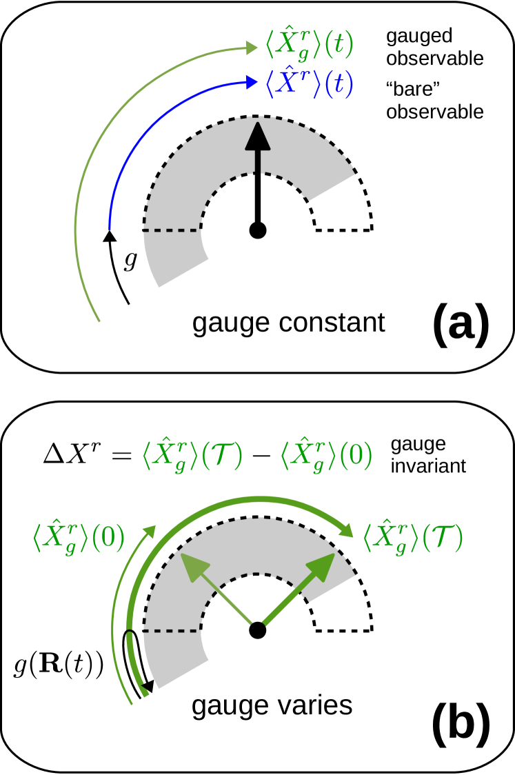
Figure 1: (a) Global gauge transformation $\hat{X}^{r}\to\hat{X}^{r}_{g}=\hat{X}^{r}+g\mathds{1}$ leaving both currents $I_{X^{r}}$ and transported observable $\Delta X^{r}$ invariant. The gray scalebar is translated by fixed amount $g$ relative to the ungauged one ($g=0$, dashed outline). The needle corresponds to the quantum state that from the observable $\hat{X}^{r}_{g}$ the measurement expectation value ${\langle{\hat{X}^{r}_{g}}\rangle}={\langle{\hat{X}^{r}}\rangle}+g$ indicated. (b) Local gauge transformation $\hat{X}^{r}\to\hat{X}^{r}_{g}=\hat{X}^{r}+g[{\mathbf{R}}]\mathds{1}$, changing the currents to $I_{X^{r}_{g}}$ but leaving the transported observable $\Delta X^{r}$ invariant. Since the meter scale is gauged in a continuous way as function of the parameters ${\mathbf{R}}$, it returns to its original position every period: $g[{\mathbf{R}}(\mathcal{T})]=g[{\mathbf{R}}(0)]$.

However, these global, ${\mathbf{R}}$ independent, gauge transformations are a too narrow class for the present problem of pumping: here we require only that the transported observable, the integral of the current over a driving period [Eq. (17b)], remains invariant. This allows for a much larger group of local gauge transformations: for each parameter value ${\mathbf{R}}$ we can choose a different gauge for the observable, determined by a continuous real function $g[{\mathbf{R}}]$:

$$\hat{X}^{r}[{\mathbf{R}}]\to\hat{X}_{g}^{r}[{\mathbf{R}}]=\hat{X}^{r}[{\mathbf{R}}]+g[{\mathbf{R}}]\mathbbm{1}.$$ (57)

In the physical picture of Fig. 1(b), this means that when driving ${\mathbf{R}}$ in time the scale bar on the detector is allowed to vary in time but only through the parameters. Because $g[{\mathbf{R}}]$ is continuous, this cannot affect the measurement of the pumped observable since at the end of a driving cycle the parameters, thus also the scale of the meter, has returned to its initial position: one reads off the change correctly as

$$\Delta X^{r}_{g}={\langle{\hat{X}^{r}_{g}}\rangle}(\mathcal{T})-{\langle{\hat{X}^{r}_{g}}\rangle}(0)=\Delta X^{r}$$ (58)

for any such calibration function $g$, continuous along the parameter driving curve $\mathcal{C}$. We stress that during the driving cycle the currents have changed due to the gauge transformation, which is entirely physical.

A prime example of working with such a driving-parameter-dependent observable is when one ignores (gauges away) the displacement charge currents when calculating the charge ($\hat{X}^{r}=\hat{N}^{r}$) transported through a driven quantum dot from a capacitive model Bruder and Schoeller (1994). In this case, the gauge function $g[{\mathbf{R}}]$ has the concrete physical meaning of minus the screening charge on electrode $r$ which depends on the time-dependent voltages (${\mathbf{R}}$) applied to all the terminals of the circuit (see, e.g., LABEL:Calvo12a, for a detailed discussion). We stress, however, that our considerations hold equally well for other observables $\hat{X}^{r}$, for example reservoir spin, energy, etc., for which there may be no obvious concept of displacement current or which may not be conserved.

In answer to question (i) we thus see that contained in every pumping problem there is a simple local gauge group of meter recalibrations, which is much larger than the trivial global constant shifts (56) of the observable. It is nearly always hidden since one fixes the gauge to $g[{\mathbf{R}}]=0$ as soon as one decides to work only with the “bare” observable $\hat{X}^{r}$ which is time- and parameter independent, see Eq. (28) ff. This is one of the two “naive” things that we did in deriving the AR pumping formula (48). However, we stress that our arguments so far did not invoke any “open-system” ideas or related approximations (e.g., integrating out the reservoirs, Born-Markov or adiabatic approximation). We also note that the gauge freedom (57) related to the identity operator is present for any pumping problem: it holds irrespective of the form of the parametrically time-dependent Hamiltonian $H^{\text{tot}}$. It is thus truly a gauge freedom of the nonsystem observables that emerges for any periodic driving. Thus, before having solved for, or even introduced, $\rho^{\text{i}}$ or $\rho^{\text{a}}$ it is already clear that the geometric nature of pumping is going to be associated with the freedom of calibrating the meter.

Open-system description. Now we show how this clear physical picture is reflected in the reduced density operator description, i.e., after integrating out the reservoirs. This brings in open-system aspects. For this we return to the AR pumping equations (25) and (40), and our careful discussion of partial normal ordering and current kernels in Sec. II.3.

The current kernel equation (41) replaces the Heisenberg equation for the current in the total system description Eq. (55) in our above discussion. Clearly, all observables differing by a constant lead to the same current kernel because of the time-derivative in the second term of Eq. (41). However, a time-local gauge transformation $\hat{X}^{r}[{\mathbf{R}}]\to\hat{X}^{r}[{\mathbf{R}}]+g[{\mathbf{R}}]\mathbbm{1}$ causes the current kernel (41) to transform as

$$W_{\hat{I}_{X^{r}}}\to W_{\hat{I}_{X^{r}_{g}}}=W_{\hat{I}_{X^{r}}}+\frac{d}{dt}g[{\mathbf{R}}(t)]\mathcal{I},$$ (59)

where $\mathcal{I}$ denotes the identity superoperator. For any gauge function $g[{\mathbf{R}}]$ this current kernel produces the same transported observable

$$\Delta{X}^{r}_{g}=\int_{0}^{\mathcal{T}}dt\mathsf{Tr}W_{\hat{I}_{X^{r}_{g}}}[{\mathbf{R}}(t)]\left[\rho^{\text{i}}(t)+\rho^{\text{a}}(t)\right]=\Delta X^{r}$$ (60)

by virtue of the probability normalization of Eq. (42) [implying $\mathsf{Tr}\rho^{\text{a}}(t)=0$] and the continuity $g[{\mathbf{R}}(\mathcal{T})]=g[{\mathbf{R}}(0)]$.

Although the transported observable is gauge invariant the current kernel that produces it is not (as we changed the meter gauge). To relate this to the observable as in (57), or rather of its expectation values, requires a little extra effort in the open system picture. To this end we separate the current in Eq. (60),

$$I_{X^{r}_{g}}(t):=\mathsf{Tr}\,W_{\hat{I}_{X^{r}_{g}}}[{\mathbf{R}}(t)]\left[\rho^{\text{i}}(t)+\rho^{\text{a}}(t)\right],$$ (61)

into an instantaneous, gauge independent part

$$I_{X^{r}}^{\text{i}}(t):=\mathsf{Tr}\,W_{\hat{I}_{X^{r}}}[{\mathbf{R}}(t)]\rho^{\text{i}}(t),$$ (62)

and a remaining adiabatic-response part that is gauge dependent:

$$I_{X^{r}_{g}}^{\text{a}}(t) :=I_{X^{r}_{g}}(t)-I_{X^{r}}^{\text{i}}(t),$$ (63a)

$$=\mathsf{Tr}\,W_{\hat{I}_{X^{r}}}[{\mathbf{R}}(t)]\rho^{\text{a}}(t)+\frac{d}{dt}g[{\mathbf{R}}(t)].$$ (63b)

As before, the labels “a” or “i” indicate whether the current component depends on $\dot{{\mathbf{R}}}(t)$ or not. Now we can identify the geometric part of the expectation value of the gauged nonsystem observable by splitting it up at any time $t$ as ${\langle{\hat{X}^{r}_{g}}\rangle}(t)={\langle{\hat{X}^{r}}\rangle}^{\text{i}}(t)+{\langle{\hat{X}^{r}_{g}}\rangle}^{\text{a}}(t)$ into an instantaneous, gauge independent part

$${\langle{\hat{X}^{r}}\rangle}^{\text{i}}(t)-{\langle{\hat{X}^{r}}\rangle}(0) :=\int_{0}^{t}d\tau I_{X^{r}}^{\text{i}}(\tau),$$ (64)

and an adiabatic-response part that contains the gauge dependence:

$${\langle{\hat{X}^{r}_{g}}\rangle}^{\text{a}}(t)-{\langle{\hat{X}^{r}}\rangle}(0) =\int_{0}^{t}d\tau I_{X^{r}_{g}}^{\text{a}}(\tau).$$ (65)

We stress that here we do not integrate over a driving period, but up to any time $t$ within the driving period, $0\leq t\leq\mathcal{T}$. Thus, after integrating out the reservoirs the gauge dependence of the total system operator $\hat{X}^{r}_{g}=\hat{X}^{r}+g\mathbbm{1}$ resides in the adiabatic-response part of the observable

$${\langle{\hat{X}^{r}}\rangle}^{\text{a}}(t)\to{\langle{\hat{X}^{r}_{g}}\rangle}^{\text{a}}(t)={\langle{\hat{X}^{r}}\rangle}^{\text{a}}(t)+g[{\mathbf{R}}(t)].$$ (66)

and not in the instantaneous one ${\langle{\hat{X}^{r}}\rangle}^{\text{i}}$. This is the open system equivalent of Eq. (57) that we sought.

Unphysical redundancy. At this point, it is important (cf. Sec. V.1) to note that the current kernel has an additional, completely unrelated redundancy that may obscure the above clear physical picture. Even when fixing the gauge $g[{\mathbf{R}}]$ of the observable $\hat{X}^{r}$, the associated current kernel is still not unique: one can always add to it a time-dependent system superoperator $\Theta(t)$,

$$W_{\hat{I}_{X^{r}}}\to W_{\hat{I}_{X^{r}}}+\Theta(t),$$ (67)

for which $\mathsf{Tr}\Theta(t)\bullet=0$, without changing any expectation value, including the AR part ${\langle{\hat{X}^{r}_{g}}\rangle}^{\text{a}}(t)$. We actually made use of this when writing the current kernel in the form (30). Importantly, this redundancy is independent of the physical gauge freedom and need not be considered further until we discuss the FCS approach [cf. Eq. (94)].

Geometric nature of pumping. Thus, the geometric nature of pumping in open systems emerges naturally when one considers the current of the transported observable, i.e., via the route Eq. (17b). In the total (open) system description, the gauge freedom lies in the nonunique association of (the adiabatic-response part of) the transported observable $\Delta X^{r}$ ($\Delta X^{r,\text{a}}$) with a current (kernel super-) operator $\hat{I}_{X^{r}_{g}}$ ($W_{\hat{I}_{X^{r}_{g}}}$).

Associated with the measurable transported observable is thus a whole class of different, parametrically time-dependent observables $\hat{X}^{r}_{g}$. We see that the space in which the physical pumping problem is solved is correspondingly much larger than thought initially based on our “naive” calculation in Sec. II.4. More precisely, it has the structure of a simple fiber-bundleNakahara (2003), sketched in Fig. 2. To each driving parameter ${\mathbf{R}}$ in the base space is attached a “copy” of the space of all possible gauge-equivalent, adiabatic-response expectation values of the observable, i.e., all possible gauge choices (66) for fixed ${\mathbf{R}}$. For the “vertical” coordinate in this space we can just take $g[{\mathbf{R}}]$, i.e., our simple fiber is isomorphic to the real line. This reflects the direct physical meaning of the real-valued $g[{\mathbf{R}}]$ as a calibration of the meter scale of Fig. 1.

As in many other areas of physics Marsden et al. (1990); Marsden and Ostrowski (1998); Cendra et al. (2001); Bloch (2003); Andersson (2003a) where one solves a physical problem in such a fiber-bundle space, a geometric phase is expected to emerge. Viewed in this larger space it is now clear from the start that there is “room” for a geometric phase to develop along the “vertical” fiber direction of the observable, even though there is no “Berry phase” in the time-dependent steady-state evolution of the mixed-state (Sec. III.1).

Returning to Fig. 2, we can visualize most clearly in what way the geometric origin of pumping effects remains hidden if one starts from the “bare”, time-independent observable operator and / or enforces partial normal-ordering of the current operator (cf. Sec. II.3). These technical assumptions physically amount to working in the fixed gauge $g=0$. Geometrically, this corresponds to using a special coordinate system relative to the plane in the sketches in Fig. 2 and Fig. 3. However, all smooth coordinate systems in this space are physically meaningful and equivalent for pumping.

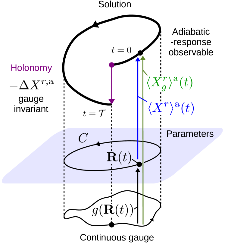
Figure 2: Fiber bundle space in which the pumping problem Eq. (68)-(69) is solved: the plane corresponds to the base space of driving parameters ${\mathbf{R}}$ containing the driving curve $\mathcal{C}$. The “vertical” space at each point ${\mathbf{R}}$ is formed by all adiabatic-response expectation values (66), ${\langle{\hat{X}^{r}_{g}}\rangle}^{\text{a}}$, each coordinatized by a real value of $g[{\mathbf{R}}]$ at that point ${\mathbf{R}}$.

III.3 Landsberg’s geometric pumping connection

Having answered question (i) by identifying the gauge freedom (the fiber bundle relevant for pumping) we will now answer question (ii): we show how the solution of the pumping problem determines a geometric connection whose geometric phase is just the pumped observable. This determines the actual magnitude of this geometric phase effect allowed by gauge freedom. Following the AR approach, the pumping problem is described by two equations (cf. Secs. II.2 and II.3), the state evolution

$$\partial_{t}{|{\rho(t)})}=W[{\mathbf{R}}(t)]\,{|{\rho(t)})}$$ (68)

exhibiting a unique frozen-parameter stationary state, $W[{\mathbf{R}}]{|{\rho^{\text{i}}})}=0$, and a second equation for a variable “enslaved” to this, the gauge-dependent current

$$\frac{d}{dt}{\langle{\hat{X}^{r}_{g}}\rangle}(t)={({\mathbbm{1}}|}W_{\hat{I}_{X^{r}_{g}}}[{\mathbf{R}}(t)]{|{\rho(t)})}.$$ (69)

Such pumping equations fit Sinitsyn (2009) into Landsberg’s general framework of nonlinear, dissipative dynamics with a symmetry Landsberg (1992, 1993), extended in Andersson (2003a, 2005) to the non-Abelian case. In our special case, the symmetry is an Abelian gauge freedom expressing changes of the coordinate system in the fiber bundle space as in Fig. 2. Moreover, our dynamics is linear as we have emphasized by introducing Liouville-space vector notation for operators and linear functions of operators, respectively:

$${({\mathbbm{1}}|}:=\mathsf{Tr},\qquad{|{\rho})}=\rho.$$ (70)

Here, we highlight the two most relevant aspects of Landsberg’s framework:

(a) Equation (68) alone does not exhibit a geometric phase, i.e., in the time-dependent steady-state limit the solution should be continuous [see Eq. (54)]. For a unique stationary state that we consider here, we showed in Sec. III.1 that this is always the case due to the general constraint of probability normalization.

(b) The variable ${\langle{\hat{X}^{r}_{g}}\rangle}(t)$, enslaved to the dynamics of the state $\rho(t)$, is not geometric as whole: only its adiabatic-response part is geometric, as noted above. However, even for this part to make sense in differential geometry, the enslaved equation (69) needs to transform in a specific way, as emphasized in LABEL:Andersson03thesis. If this were not the case, pumping could not be related to a connection and curvature, the basic concepts for relating physical results to geometric and topological properties of a fiber bundle. In our case, this corresponds to the physical transformation law for the current kernel Eq. (59), which is essentially the Heisenberg equation of motion after integrating out the reservoirs.

Following Refs. Andersson, 2003a, 2005, in Landsberg’s approach one solves Eqs. (68) and (69) for the time-dependent steady state using the AR procedure, now including the gauge dependence in contrast to Eqs. (25)-(40), and extracts a geometric phase that is thus a leading-order nonadiabatic effect (adiabatic response). Proceeding as before in Sec. II.4, we compute $\rho^{\text{i}}$ and $\rho^{\text{a}}$ and insert these into Eqs. (62) and Eq. (63b). This gives for the instantaneous part of the transported observable

$$\Delta X^{r,\text{i}}=\int^{\mathcal{T}}_{0}dtI^{\text{i}}_{X^{r}}(t)=\int_{0}^{\mathcal{T}}dt{({\mathbbm{1}}|}W_{\hat{I}_{X^{r}}}[{\mathbf{R}}(t)]{|{\rho^{i}})},$$ (71)

which is equal to Eq. (46). However, the adiabatic-response correction now reads as

$$\Delta X^{r,\text{a}}=\int^{\mathcal{T}}_{0}dtI^{\text{a}}_{X^{r}_{g}}(t)=\oint_{\mathcal{C}}d{\mathbf{R}}A_{g}[{\mathbf{R}}],$$ (72)

where using Eq. (41) we introduced the expressions

$$A_{g} :=A_{0}[{\mathbf{R}}]+{\mathbf{\nabla_{R}}}g[{\mathbf{R}}],$$ (73a)

$$A_{0}[{\mathbf{R}}] ={({\mathbbm{1}}|}W_{\hat{I}_{X^{r}}}[{\mathbf{R}}]\frac{1}{W[{\mathbf{R}}]}{\mathbf{\nabla_{R}}}{|{\rho[{\mathbf{R}}]})}.$$ (73b)

The pumping is now explicitly seen to be geometric, in a more restricted sense, since we have now formulated the problem without inadvertently fixing a gauge. It is now clear why “adding a differential under the integral” must physically always be possible: it is a meter recalibration. Answering question (ii), the pumped observable (72) is indeed a geometric phase determined by $A_{g}$, which, as we discuss below, plays the role of a geometric connection with a clear physical motivation. By Eq. (59) the gauge potential $A_{g}$ indeed shows the proper transformation to a new gauge with the simple additive gauge group $\sim\mathds{R}$ of meter recalibrations:

$$A_{f}[{\mathbf{R}}]\rightarrow A_{f+g}=A_{f}[{\mathbf{R}}]+{\mathbf{\nabla_{R}}}g[{\mathbf{R}}].$$ (74)

This ensures that the pumped observable is gauge invariant, even though it is computed from the gauge-dependent adiabatic-response part of the current $I_{X^{r}_{g}}(t)\propto\dot{{\mathbf{R}}}(t)$.

When applying our considerations to the simpler case of pumping of system observables and a single reservoir our formulation recovers the geometric pumping result of Avron et al.Avron et al. (2012a) for the case of a unique stationary state. This is worked out in Appendix E, further showing the complementarity to LABEL:Avron12 which inspired the above.

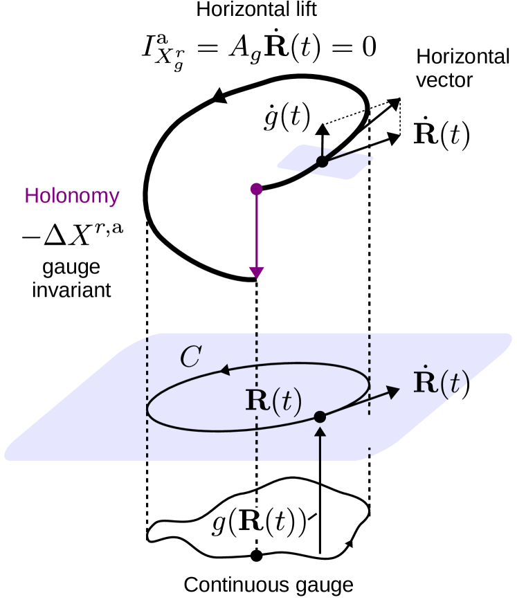
Figure 3: In a fiber-bundle space, the notion of what is “horizontal” is completely undefined, in contrast to “vertical,” which is naturally the direction along gauge coordinate $g$, the fiber space. “Horizontal” cannot be defined as orthogonal to “vertical”, since there is no physically motivated metric in this space. However, the function $A_{g}[{\mathbf{R}}]$ arising in the solution of the physical pumping problem of Eqs. (68) and (69) can be used to define what “horizontal” means at each point, thus defining a geometric “connection.” The nonintegrability of the connection $A_{g}$ leads to the discontinuity in the horizontal lift of the curve $\mathcal{C}$ into the bundle space. This is the differential-geometric significance of Landsberg’s connection for pumping.

III.4 Physical meaning of horizontal lift,
parallel transport and holonomy

The answer to question (ii), i.e., that pumping defines a geometric connection, can be further clarified by considering the physical meaning of key concepts of differential geometry of the fiber bundle of meter calibrations. In this regard, the connection (73a) has the advantage that it is a global connection Nakahara (2003), i.e., defined in the total space of the fiber bundle (in contrast to local connection forms independent of the gauge coordinate). This global object has the most direct geometric significance, which is also why it is favored in differential geometry. Also, physically it is most revealing as we now explain.

The central notion of “horizontal space” in a fiber bundle, can be defined directly by requiring this connection [a linear function of vectors in the total space, $(\dot{{\mathbf{R}}},\dot{g})$, transforming as (74)] to vanish. Since we avoid the use of differential forms, this should be written as

$$I^{\text{a}}_{X^{r}_{g}}(t) =A_{g}[{\mathbf{R}}(t)]\dot{{\mathbf{R}}}(t)$$

$$=A_{0}[{\mathbf{R}}(t)]\,\dot{{\mathbf{R}}}(t)+\dot{g}\,[{\mathbf{R}}(t)]=0.$$ (75)

This locally determines a linear relation between a direction in the base parameter space ($\dot{{\mathbf{R}}}$) and the “vertical” gauge direction ($\dot{g}$). This is sketched in Fig. 3. From the point of view of differential geometry, the pumping current can thus be used to define the notion of a “horizontal” direction in the total space. Moving tangent to this so-defined “horizontal” space is called “parallel transport” and by Eq. (75) physically corresponds to maintaining zero pumping current as the measurement proceeds. We stress that this zero-current condition Eq. (75) derives ultimately from physics, i.e., from the state evolution [Eq. (68)] plus the open-system Heisenberg equation of motion [Eq. (69)]: it is not imposed. This is illustrated in Fig. 4 : one calibrates the meter’s scale in a parameter-dependent way such that the needle always indicates a fixed expectation value for $\hat{X}^{r}_{g}$ relative to this moving scale.

From the sketch of these calibrations in Fig. 4 it is clear that, if there is a nonzero pumping effect, this condition cannot be maintained in a continuous way along the closed driving curve $\mathcal{C}$: the “vertical” jump at ${\mathbf{R}}(0)={\mathbf{R}}(\mathcal{T})$ is the cumulative calibration required to maintain zero current during the driving period. This calibration must equal minus the pumped value. To see this, let $h(t)$ denote the curve that solves the differential equation (75) along the closed base space curve $\mathcal{C}$. This curve is known as the “horizontal lift” of $\mathcal{C}$ in Fig. 3. Substituting $g[{\mathbf{R}}(t)]\to h(t)$, we find for the discontinuity:

$$h(\mathcal{T})-h(0)=-\oint_{\mathcal{C}}d{\mathbf{R}}A_{0}[{\mathbf{R}}]=-\Delta X^{r,\text{a}}.$$ (76)

This discontinuity is the geometric phase or the “holonomy” of the horizontal lift. Indeed, in the present problem this is just minus the pumped observable.

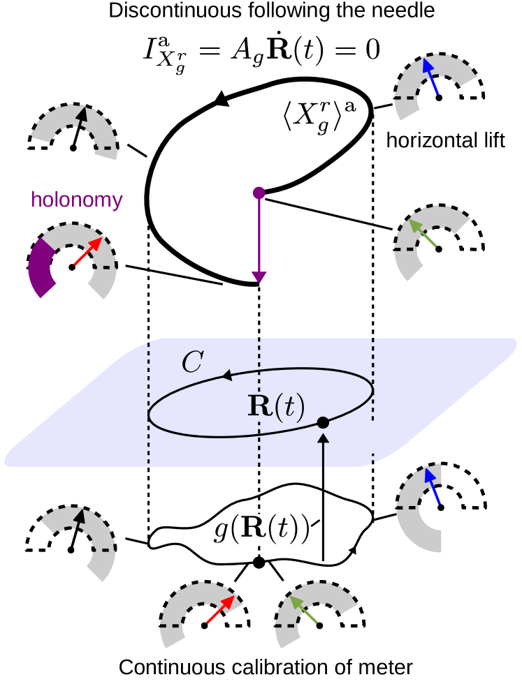
Figure 4: Physical meaning of differential geometric notions of Fig. 3 in the pumping problem. The linear space defined by the connection [Eq. (75)] locally determines a plane of “horizontal” vectors in Fig. 3. Pumping corresponds to “parallel transporting” such a vector thereby producing a “horizontal lift” of the closed parameter drive curve $\mathcal{C}$. Physically, this signifies that one calibrates the meter for the observable, drawn in same way as in Fig. 1, such that one maintains zero pumping-current $I_{X^{r}_{g}}^{\text{a}}$ in this gauge. If there is pumping (the connection is nonintegrable) the lifted curve “breaks” as shown in Fig. 3. Physically, the “vertical” discontinuity, the holonomy, is minus the pumped observable, i.e., the cumulative calibration (purple) required to maintain zero current during one driving period. Along the horizontal lift, the scale (grey) is made to follow the pointer.

In summary, by starting from the gauge freedom in a system plus reservoir description we arrived at the tangible physical meaning for all the relevant geometric notions that arise in the reduced density operator description of steady-state pumping. By simply formulating the AR calculation of pumping in the physically natural larger fiber-bundle space, it becomes clear that there is always room for a geometric pumping phase to develop for any nonsystem observable. Physically, this is just the space that includes all possible meter gauges. Although in the present case the actual calculations are all easy, this simple picture has received little attention so far. Much attention has been given to the more general but also more complicated geometric FCS approach. The relative simplicity of Landsberg’s approach is a crucial advantage when addressing more complicated models and dynamics Wegewijs et al. .

IV Pumping curvature

We now turn to question (iii) posed in Sec. II.5 by analyzing necessary conditions for the pumped observable in the AR approach to be nonzero.

IV.1 Pumping curvature and response covector

It is useful to rewrite the pumped observable (72) as a surface integral over a curvature $B_{X^{r}}[{\mathbf{R}}]={\mathbf{\nabla_{R}}}\times A_{X^{r}}[{\mathbf{R}}]$:

$$\Delta X^{r,\text{a}}=\int_{\mathcal{S}}dSB_{X^{r}}.$$ (77)

By working with dimensionless parameters ${\mathbf{R}}$, this curvature has the direct physical meaning of pumped observable per unit area of the driving parameter space. In view of the following discussion, we now explicitly indicate the considered observable $X^{r}$ in the curvature $B$. Clearly, adiabatic-response pumping always requires at least two parameters to be driven. Otherwise, the driving curve $\mathcal{C}$ does not bound a surface $\mathcal{S}$ and Eq. (77) gives a zero result. This rules out all driving schemes that are trivial one-dimensional curves in parameter space.

Given the driving cycle is two dimensional, we investigate when the integrand, i.e., the pumping curvature $B_{X^{r}}[{\mathbf{R}}]$, is nonzero by writing it in the transparent form

$$B_{X^{r}}[{\mathbf{R}}]={({{\mathbf{\nabla_{R}}}\Phi_{X^{r}}[{\mathbf{R}}]}|}\times{|{{\mathbf{\nabla_{R}}}\rho^{\text{i}}[{\mathbf{R}}]})}$$ (78)

deriving from the Landsberg connection (73). We define $(a\times b)_{ij}:=a_{i}b_{j}-a_{j}b_{i}$ component-wise, which in two dimensions corresponds to the cross-product vector that is normal to the parameter plane. Extending ideas of LABEL:Calvo12a [cf. also Appendix F], here we introduced an adiabatic-response covector :

$${({\Phi_{X^{r}}[{\mathbf{R}}]}|}:={({\mathds{1}}|}W_{\hat{I}_{X^{r}}}[{\mathbf{R}}]\frac{1}{W[{\mathbf{R}}]}.$$ (79)

That the Landsberg curvature (78) is explicitly gauge invariant [cf. (73)], indicates that it has a direct physical interpretation as a pumped observable: by Eq. (77) $B_{X^{r}}[{\mathbf{R}}]$ is the pumped observable per unit area of the parameter space, i.e., bounded by an infinitesimal pumping cycle at ${\mathbf{R}}$. Thus, the pumping curvature can be experimentally obtained in the limit of small amplitude driving as $B_{X^{r}}=d(\Delta X^{r,\text{a}})/d\mathcal{S}$.

The response covector (79) has a physically transparent form: a nonzero pumping curvature (78) necessarily requires that the combined effect of the “lag time” of the retarded mixed quantum state (pseudo-inverse relaxation kernel $W^{-1}$) together with the observable current (current kernel $W_{\hat{I}_{X^{r}}}$) is parameter dependent.

The cross product in Eq. (78) imposes a stringent condition: the pumping curvature does not only vanish when the gradient of the response-covector itself is zero but also when it is parallel to the parametric gradient of the stationary-state, schematically:

$${\mathbf{\nabla_{R}}}\Phi_{X^{r}}[{\mathbf{R}}]\quad\parallel\quad{\mathbf{\nabla_{R}}}\rho^{\text{i}}[{\mathbf{R}}].$$ (80)

Here, the gradients are vectors obtained from each ${\mathbf{R}}$-dependent matrix element of the two operators in the cross product in Eq. (78). Expanding both operators in a basis one obtains a Brouwer-type formula (see Appendix F), which shows that for a nonzero result it is necessary that in this expansion at least some components of the two operators should pairwise have nonparallel gradients. In general this is not yet sufficient since in the sum they may cancel. An explicit example of the curvature for an interacting quantum dot is is given in Eq. (190).

IV.2 Geometric spectroscopy

The schematic condition (80) forms the basis for the adiabatic-response pumping spectroscopy proposed in Reckermann et al. (2010); Calvo et al. (2012); Haupt et al. (2013) in the specific setting of quantum dots. Here we outline how this spectroscopy works in more general terms, indicating that it extends to a much broader class of open systems.

The physical idea is the following: in Eq. (80) clearly both the kernel $W[{\mathbf{R}}]$, defining $\rho^{i}[{\mathbf{R}}]$ [Eq. (43a)], and the current kernel $W_{\hat{I}_{X^{r}}}$, defining $\Phi_{X^{r}}[{\mathbf{R}}]$ [Eq. (79)], depend on the spectral properties of the closed system, the Hamiltonian $H$, and of the reservoirs, $H^{\text{res}}$. Due to the weak coupling to the reservoirs strong variations of these two quantities as function of the parameters ${\mathbf{R}}$ are expected when the driving curve $\mathcal{C}$ hits a parameter point for which the system is in energetic resonance with the reservoirs. For particle transport, for example, this happens when the electrochemical potential of one of the reservoirs lines up with one of the system’s particle-addition energies. When only such a single-resonance parameter value is traversed by the driving curve, the ${\mathbf{R}}$-dependence is thus effectively one dimensional i.e., effectively we drive a single parameter. We then have the situation (80) of effective one-parameter driving and the adiabatic-response is zero on general grounds.

However, the driving may also visit parameter values where the system simultaneously satisfies two (or more) resonance conditions. For example, two or more system addition energies may line up with electrochemical potentials of two reservoirs. Then the ${\mathbf{R}}$-dependence of the operators $\Phi_{X^{r}}[{\mathbf{R}}]$ and $\rho^{i}[{\mathbf{R}}]$ in Eq. (80) will in general be different, giving the necessary lifting of condition (80) for zero-pumping: the magnitude of the pumping curvature is thus generically expected to show a peak at crossings of resonances.

Indeed, in quantum dots this leads to a sharp pattern of “spots” Reckermann et al. (2010); Calvo et al. (2012); Yoshii and Hayakawa (2013); Haupt et al. (2013) at the crossings of single-resonance parameter lines in the plane of applied voltages (“stability diagram”) when plotting $B[{\mathbf{R}}]$. However, as the above argument indicates, the idea is more general: a recording of $\Delta X^{r,\text{a}}$ or $B_{X^{r}}$ as function of the driving parameter working point ${\mathbf{R}}$ contains detailed information on the open system, both through its sign and magnitude. Some of this information is not contained in the instantaneous transported observable $\Delta X^{r,\text{i}}$. For example, in an interacting quantum dot the sign of the curvature reveals the spin-degeneracy through pumping (without using a magnetic field) as well as the direction of the junction asymmetry Reckermann et al. (2010). Also, different pumping observables have different resolving capabilities: for example, some resonances that are hidden in charge pumping are revealed by spin pumping Calvo et al. (2012); Haupt et al. (2013).

The basic principle of the geometric spectroscopy is thus to probe the system’s properties via its leading parameter-dependence in adiabatic-response to slow driving rather than to more drastic physical excitation. The pumping formula Eq. (78) provides a straightforward approach for computing the detailed response for a variety of systems and observables Pluecker et al. , illustrated in Appendix D for a driven quantum dot. In general this formula can be written in a Brouwer-type Brouwer (1998) form with additional terms (see Appendix F). Before we discuss simplifications of this formula in more special situations, we stress its generality: It holds, within our approximations, for any weakly-coupled open quantum system, e.g., comprised of many orbitals with arbitrary interactions [as described by $H$ in Eq. (13)].

IV.3 Pumping of conserved observables

The Landsberg pumping curvature (78) has the advantage that it can easily be simplified when the considered nonsystem observable $\hat{X}^{r}$ is conserved by the coupling [Eq. (13)] at junction $r$ for each traversed parameter value:

$$[\hat{X}[{\mathbf{R}}]+\hat{X}^{r},V^{r}[{\mathbf{R}}]]=0.$$ (81)

Here $\hat{X}[{\mathbf{R}}]$ is the corresponding system observable. As for the reservoirs [cf. Eq. (35)], we assume that this observable is also conserved inside the system (in the absence of coupling):

$$[{H}[{\mathbf{R}}],\hat{X}[{\mathbf{R}}]]=0.$$ (82)

Examples are the charge ${N}^{r}+{N}$ for a tunnel junction to a normal-metal electrode or the spin ${S}_{z}^{r}+{S}_{z}$ for a nonmagnetic tunnel junction to a ferromagnetic electrode with polarization in $z$ direction. In these cases, both observables are ${\mathbf{R}}$ independent.

However, Eq. (81) allows that the conservation law yields a system observable that does depend on ${\mathbf{R}}$, even though $\hat{X}^{r}$ is ${\mathbf{R}}$-independent. The prime example for this is the pumping of heat where in ${H}^{r}[{\mathbf{R}}]-\mu^{r}[{\mathbf{R}}]{N}^{r}$ the ${\mathbf{R}}$-dependence may cancel out between the two terms, as we assumed in Eq. (14), but the corresponding system observable ${H}[{\mathbf{R}}]-\mu^{r}[{\mathbf{R}}]{N}$ is still ${\mathbf{R}}$ dependent. We stress that this parameter dependence cannot be gauged away since it is in general not of the form $g[{\mathbf{R}}]\mathbbm{1}$ and thus contributes to both the instantaneous and the adiabatic-response of the transported observable. Our considerations apply to this case as well deserving a separate study Pluecker et al. .

The conservation law (81) together with Eq. (82) implies that the computation of $W_{\hat{I}_{X^{r}}}$ can be avoided by using

$${({\mathbbm{1}}|}\,W_{\hat{I}_{X^{r}}}[{\mathbf{R}}]=-{({X[{\mathbf{R}}]}|}\,W^{r}[{\mathbf{R}}].$$ (83)

Notably, on the right hand side, $\hat{X}$ is the system observable and $W^{r}$ is the part of the known time-evolution kernel due to the coupling $V^{r}$ to reservoir $r$ alone. The latter is easily obtained from $W$ as given by Eq. (26) by dropping $L$ and also all contributions from reservoirs $r^{\prime}\neq r$. We stress that in order to use Eq. (83) only conservation at junction $r$ is required, not at all junctions.

The relation (83) is derived in Appendix A using the same assumptions and the same approach as in Secs. II.2 and II.3. Its use is illustrated in Eq. (186). For weak-coupling and memoryless master equations this relation is well-known in a less convenient form discussed in Appendix B. The form (83) has the advantage of having a very similar exact generalization Saptsov and Wegewijs (2012) that relies only on the decomposition of the coupling as $V=\sum_{r}V^{r}$, allowing the present considerations to be extended Wegewijs et al. .

Using Eq. (83) the response vector (79) simplifies to

$${({\Phi_{X^{r}}[{\mathbf{R}}]}|}=-{({X[{\mathbf{R}}]}|}W^{r}[{\mathbf{R}}]\frac{1}{W[{\mathbf{R}}]}.$$ (84)

Physically, $W^{r}W^{-1}$ describes the “fraction of $\hat{X}$” in the system that flows through the junction to reservoir $r$ where it “ turns into $\hat{X}^{r}$ ”. Combined with Eq. (78) we see that the ${\mathbf{R}}$-dependence of this fraction is the decisive factor for the pumping of a conserved observable:

$$B_{X^{r}}[{\mathbf{R}}]=$$

$$-{({X[{\mathbf{R}}]}|}\Big{[}{\mathbf{\nabla_{R}}}W^{r}[{\mathbf{R}}]\frac{1}{W[{\mathbf{R}}]}\Big{]}\times{|{{\mathbf{\nabla_{R}}}\rho^{\text{i}}[{\mathbf{R}}]})}$$ (85a)

$$-{({{\mathbf{\nabla_{R}}}X[{\mathbf{R}}]}|}W^{r}[{\mathbf{R}}]\frac{1}{W[{\mathbf{R}}]}\times{|{{\mathbf{\nabla_{R}}}\rho^{\text{i}}[{\mathbf{R}}]})}.$$ (85b)

The second term is entirely due to the above mentioned possible parameter dependence of the “bare” (ungauged) observable. It is absent for constant $\hat{X}[{\mathbf{R}}]=\hat{X}$ such as charge or spin. In this case the remaining term Eq. (85a) nicely shows that nonzero pumping requires spatial symmetry breaking. For example, for two reservoirs one expects that some electric or thermal bias or different coupling strengths at the two junctions is needed to break spatial symmetry for at least some of accessed parameters ${\mathbf{R}}$. Otherwise, there is no net preferred direction of transporting charge and the time-dependent charge current averages out over one pumping cycle. This is clearly expressed by Eqs. (84) and (85a): in such a case the kernels $W^{r}[{\mathbf{R}}]$, $W[{\mathbf{R}}]$ are proportional, i.e., the fraction $W^{r}[{\mathbf{R}}]W[{\mathbf{R}}]^{-1}$ is constant. The curvature then vanishes because the covector is zero [not just parallel to ${\mathbf{\nabla_{R}}}\rho^{\text{i}}$ as in Eq. (80)]:

$${({{\mathbf{\nabla_{R}}}\Phi_{X^{r}}[{\mathbf{R}}]}|}=0.$$ (86)

This then implies that there is no pumping of any such conserved, constant observable $\hat{X}$. For example, for a quantum dot with symmetric coupling to two normal metal electrodes $r=\text{L},\text{R}$ one finds $W^{r}[{\mathbf{R}}]W[{\mathbf{R}}]^{-1}=\tfrac{1}{2}\mathcal{I}$ independent of ${\mathbf{R}}$ and $r$. As a result, ${({\Phi_{X^{r}}}|}=-\tfrac{1}{2}{({X}|}=-\tfrac{1}{2}\mathsf{Tr}\,\hat{X}$ for the quantum dot observables such as charge (${N}$) and spin (${S}_{x}$, ${S}_{y},$ or ${S}_{z}$).

Finally, we note that the term (85a) can also be related to the expressions for the simple case of pumping of system observables obtained using the AR approach of LABEL:Avron12, see Appendix E.

V Full counting statistics approach to geometric pumping

We have completed our discussion of the Landsberg-AR framework for geometric pumping. Now we turn to the final question (iv) raised in Sec. II.5 by comparing this approach with the established geometric FCS density-operator approach Sinitsyn and Nemenman (2007a), which has been applied to various problems Sinitsyn and Nemenman (2007a); Ren et al. (2010); Yuge et al. (2012); Liu et al. (2013); Yuge et al. (2013); Nakajima et al. (2015). We first review its formulation for arbitrary moments of an observable $\hat{X}^{r}$, making the same general assumptions as we made in Sec. II. Then we highlight some insights offered by the close analogy to Sarandy and Lidar’s earlier geometric ASE approach to adiabatic mixed-state evolution Sarandy and Lidar (2005). Then, focusing on the first moment only, we discuss how the FCS formalism reduces exactly to the Landsberg-AR approach: first by giving a very simple a priori argument and then by simplifying the explicit FCS expressions using standard perturbation theory in the counting field $\chi$. Using the latter explicit relation, we show how the clear picture of the physical gauge freedom in pumping obtained in the AR approach can be transferred to the FCS approach. Finally, we discuss how the “adiabatic Berry phase” of the FCS can produce pumping effects of nonadiabatic origin and how the corresponding “adiabatic” restriction on the driving relates to this.

V.1 FCS density-operator approach

The core idea of the full counting statistics density-operator approach Bagrets and Nazarov (2003); Esposito et al. (2009a) is to describe transport processes by studying a single object, a generating function $Z^{\chi}(t)$. This function incorporates the statistics for all moments of a selected reservoir observable $\hat{X}^{r}$ (or several Nakajima et al. (2015)). Its use is thus broader than the AR approach based on the master equation (25) complemented by an observable current kernel (40). Instead of taking the route via Eq. (17b) by focusing on the current $d\hat{X}^{r}/dt$, the FCS approach follows the route via Eq. (17a), computing the cumulative change of the expectation values of $\hat{X}^{r}$ between time $t$ and an initial time $t_{0}$. In fact, the FCS generalizes the transported observable Eq. (17a) to all moments $n=0,1,2,\ldots$

$$(\Delta{X}^{r})^{n}(t):=\langle\hat{T}\left(\hat{X}^{r}(t)-\hat{X}^{r}(t_{0})\right)^{n}\rangle,$$ (87)

where $\hat{T}$ denotes time ordering and $\hat{X}^{r}(t)$ is the Heisenberg-picture operator. It is obtained from the generating function $Z^{\chi}(t)$ by

$$(\Delta{X}^{r})^{n}(t)=\partial^{n}_{i\chi}\left.Z^{\chi}(t)\right|_{\chi=0},$$ (88)

taking the steady-state limit $t_{0}\to-\infty$ [cf. Eq. (17) ff.]. Here the variable $\chi\in(-\pi,\pi)$ is the counting field and we use the shorthand $\partial_{i\chi}:=-i\partial/\partial\chi$. Although we will not indicate this, it is important to keep in mind that $Z^{\chi}$, and below any object depending on $\chi$, is specific to the selected observable $\hat{X}^{r}$.

The function $Z^{\chi}(t)$ is a transform of the probability density $P(t;\Delta X^{r})$ to obtain a change $\Delta X^{r}$ in the discrete two-point measurement outcomes of observable $\langle\hat{X}^{r}\rangle$ at the start and end of the time-interval $[t_{0},t]$:

$$Z^{\chi}(t):=\int d\Delta X^{r}P(t;\Delta X^{r})e^{i\chi\Delta X^{r}}.$$ (89)

In the following some general properties will be important: (a) normalization of the probability distribution $P(t;\Delta X^{r})$ implies at $\chi=0$

$$\left.Z^{\chi}(t)\right|_{\chi=0}=1\text{ for all $t\geq t_{0}$}.$$ (90)

(b) Hermiticity of the observable $\hat{X}^{r}$ requires

$$[Z^{\chi}(t)]^{*}=Z^{-\chi}(t)\text{ for all $t\geq t_{0}$ and all $\chi$}.$$ (91)

(c) At $t_{0}$ the changes in ${\langle{X^{r}}\rangle}$ are zero by definition (87):

$$Z^{\chi}(t_{0})=1\text{ for all $\chi$}.$$ (92)

To obtain the required time-evolution of the generating function $Z^{\chi}(t)$, one studies an auxiliary operator $\rho^{\chi}(t)$ (here referred to as generating operator) that produces this function upon tracing over the system:

$$Z^{\chi}(t)=\mathsf{Tr}\,\rho^{\chi}(t).$$ (93)

It is crucial for the following that in this step the FCS approach introduces an additional redundancy, irrelevant for the gauge freedom, in the description: $\rho^{\chi}(t)$ can be shifted by any time- and $\chi$-dependent traceless operator without altering $Z^{\chi}(t)$:

$$\rho^{\chi}(t)\to\rho^{\chi}(t)+\theta^{\chi}(t).$$ (94)

There is a corresponding redundancy also in the AR approach [cf. (67)].

As reviewed in LABEL:Esposito09rev the generating operator can in turn be expressed as

$$\rho^{\chi}(t)=\underset{\text{res}}{\mathsf{Tr}}\,\rho^{\text{tot},\chi}(t),$$ (95)

the partial trace over a generating operator $\rho^{\text{tot},\chi}(t)$ for system plus reservoir that evolves under a formal non-unitary time-evolution from the initially factorizing density operator (21):

$$\rho^{\text{tot},\chi}(t)= U^{{\chi}/{2}}(t-t_{0})\,{\rho}^{\text{tot}}(t_{0})\,[U^{-{\chi}/{2}}(t-t_{0})]^{\dagger},$$ (96a)

$$U^{\chi}(t)= e^{i\chi X^{r}}U(t)e^{-i\chi X^{r}}.$$ (96b)

where $U(t)=e^{-i(H^{0}+V)t}$. Here all driving parameters are frozen [cf. Eq. (20b)] and the limit $t_{0}\to-\infty$ is taken after the reservoir trace. This introduces a strong formal analogy of the generating operator $\rho^{\chi}(t)=\mathsf{Tr}_{\text{res}}\rho_{\text{tot}}^{\chi}(t)$ to the reduced density operator $\rho(t)$ discussed in the ASE approach will be exploited below. An elegant aspect of the FCS approach is that by the definitions (95)-(96) the quantum state evolution is included in the $\chi=0$ part of the generating operator

$$\left.\rho^{\chi}(t)\right|_{\chi=0} ={\rho(t)}\text{ for all $t\geq t_{0}$},$$ (97)

ensuring condition (90) holds,

$$\mathsf{Tr}\,\rho^{\chi}(t)|_{\chi=0}=1.$$ (98)

Furthermore the dynamics (96) ensures condition (91) by

$$\rho^{\chi}(t)^{\dagger}=\rho^{-\chi}(t)\qquad\text{ for all $\chi$}.$$ (99)

The $\chi$-independent initial condition for the dynamics

$$\rho^{\chi}(t_{0}) =\rho(t_{0})\text{ for all $\chi$}$$ (100)

guarantees condition (92). The flip side of this inclusion of $\rho(t)$ in $\rho^{\chi}(t)$ is that it becomes less clear what the “adiabatic” approximation for the formal time-evolution within the FCS approach entails physically [Sec. V.3.4]. From $\rho^{\chi}(t)$ all moments of the transported observable can be obtained by Eq. (88) and (93).

V.2 FCS approach to pumping

Born-Markov counting kernel. To calculate the generating operator $\rho^{\chi}(t)$ of the FCS we can now exploit its analogy to the quantum state $\rho(t)$ in the ASE. It allows, for example, to calculate the time-nonlocal kernels for the time-evolution of $\rho^{\chi}(t)$ using techniques developed for a quantum-state evolution kernel [cf. Eq. (11)], e.g., using Nakayima-Zwanzig projections Flindt et al. (2008); Esposito et al. (2009a) or real-time diagrams Braggio et al. (2006), with minimal modifications. Using either technique one finds in the simple Born-Markov limit that the generating operator obeys a FCS master equation Bagrets and Nazarov (2003) with the counting field $\chi$ as a formal continuous parameter:

$$\frac{\partial}{\partial t}{|{\rho^{\chi}(t)})}=W^{\chi}(t){|{\rho^{\chi}(t)})}.$$ (101)

Here we have again introduced the Liouville-space notation (70) for operators, ${\rho^{\chi}(t)}={|{\rho^{\chi}(t)})}$. The concrete expression for the FCS kernel $W^{\chi}$ is not crucial for the following. In Appendix I we give an explicit example for charge pumping through a single level quantum dot. To preserve the general properties (97) and (99) of the observable statistics the FCS kernel is restricted by, respectively,

$$W^{\chi}(t)|_{\chi=0}=W(t),$$ (102)

$$W^{\chi}(t)=KW^{-\chi}(t)K,$$ (103)

where $Kx:=x^{\dagger}$ denotes Hermitian conjugation.

Pumping. We now outline how the FCS approach applies to pumping. In this case, the driving of the parameters ${\mathbf{R}}(t)$ is responsible for the time dependence, i.e., $W^{\chi}(t)\to W^{\chi}[{\mathbf{R}}(t)]$ in Eq. (101). Instead of following the original works Refs. Sinitsyn and Nemenman, 2007a; Sinitsyn, 2009 we highlight the analogy to Sarandy and Lidar’s earlier ASE approach Sarandy and Lidar (2005, 2006) (summarized in Appendix G) which can be applied to the FCS master equation (101) with the sole modification of keeping track of the additional parameter $\chi$.

Thus, an approximate solution of the FCS master equation (101) is obtained by first diagonalizing $W^{\chi}$ for fixed parameters ${\mathbf{R}}$ (instantaneous solution) and then neglecting the couplings between different eigenspaces in the dynamics (see Appendix G). Formally similar to adiabatic state dynamics, in the steady-state limit only the left and right eigenvectors of $W^{\chi}(t)$ for the eigenvalue $\lambda^{\chi}_{0}(t)$ with largest real part are required since the contributions of all other terms are exponentially smaller. The condition for the validity of this approximation will be discussed at the end in Sec. V.3.4, clarifying what the “adiabaticity” assumed in the FCS physically entails.

Also analogous to the ASE approach is that the gauge freedom in the FCS approach lies in the freedom of choosing the eigenvectors: for every ${\mathbf{R}}$ they can be multiplied by any nonvanishing complex function of $\chi$, which we will discuss in more detail below [Eq. (132)]. We will always choose the right eigenvector for eigenvalue $\lambda^{\chi}_{0}(t)$, denoted by ${|{v^{\chi}_{0}[{\mathbf{R}}]})}$, to depend continuously on ${\mathbf{R}}$. Normalization (102) further requires that

$${({\mathds{1}|v^{\chi}_{0}[{\mathbf{R}}]})}|_{\chi=0} =1.$$ (104)

The remaining gauge freedom amounts to specifying the trace of the operator ${|{v^{\chi}_{0}})}$ as function of $\chi$. In the following we choose

$${({\mathds{1}|v^{\chi}_{0}[{\mathbf{R}}]})} =1\text{ for all $\chi$}.$$ (105)

It will turn out that by this we fix the physical gauge to the case $g=0$ of the AR formulation. We investigate other choices of the FCS gauge later on.

In addition, it follows from Eq. (103) that $\lambda^{\chi*}_{0}=\lambda^{-\chi}_{0}$ and that the operators of the right eigenvectors for opposite counting fields are related: one can always choose this eigenvector to additionally satisfy for any ${\mathbf{R}}$ and $\chi$

$$v^{\chi}_{0}[{\mathbf{R}}] =[v^{-\chi}_{0}[{\mathbf{R}}]]^{\dagger}.$$ (106)

With these choices, the “adiabatic” solution of Eq. (101) in the long time limit is given by

$${|{\rho^{\chi,\text{i}}(t)})} =Z^{\chi}(t)\,{|{v^{\chi}_{0}[{\mathbf{R}}(t)]})},$$ (107)

where we have set the initial condition $(\bar{v}_{0}^{\chi}[\mathbf{R}(0)]|\rho(0))=1$ to ensure $Z^{\chi}(0)=1$. This redefines $Z^{\chi}(t)$ to be the steady state generating function relative to $t=0$ rather than $t=t_{0}$. Only this quantity can be compared to the results of the AR approach, in which the steady state limit is taken from the start [Eq. (21) ff.]. Here, the label “i” is chosen in view of our later comparison with the AR approach (cf. Sec. V.3.4). It should be noted that after the “adiabatic” approximation the $\chi=0$ part does not keep track of the quantum state in the same way as the AR does [$\rho^{\text{a}}(t)$ is missing]. Remarkably, as we will see, it does keep track of the pumping effects Nakajima et al. (2015) in the specific observable $\hat{X}^{r}$ that in AR are caused by this missing term $\rho^{\text{a}}(t)$.

Inserting Eq. (107) as an ansatz into Eq. (101) and solving along the closed driving curve $\mathcal{C}$ traversed in period $\mathcal{T}$, one obtains

$${|{\rho^{\chi,\text{i}}({\mathcal{T}})})} =e^{\Lambda^{\chi}({\mathcal{T}})}e^{\gamma^{\chi}({\mathcal{T}})}{|{v^{\chi}_{0}[{\mathbf{R}}(0)]})}.$$ (108)

Here, the dynamical phase derives from the eigenvalue

$$\Lambda^{\chi}({\mathcal{T}}) :=\int_{0}^{\mathcal{T}}dt\lambda_{0}^{\chi}[{\mathbf{R}}(t)],$$ (109)

whereas the geometric phase is obtained as

$$\gamma^{\chi}({\mathcal{T}}) :=-\oint_{\mathcal{C}}d{\mathbf{R}}A^{\chi}[{\mathbf{R}}]$$ (110)

from the corresponding left and right eigenvector through

$$A^{\chi}[{\mathbf{R}}] ={({\overline{v}^{\chi}_{0}[{\mathbf{R}}]|{\mathbf{\nabla_{R}}}|v_{0}^{\chi}[{\mathbf{R}}]})}.$$ (111)

Geometric nature of the FCS of pumping. In geometric terms (cf. Sec. III.4), the generating operator ${|{\rho^{\chi,\text{i}}({\mathcal{T}})})}$ is, up to the dynamical factor $e^{\Lambda^{\chi}({\mathcal{T}})}$, a horizontal lift of the closed curve $\mathcal{C}$ in the driving-parameter space. In the FCS, the relevant “vertical” space attached to each parameter in the ${\mathbf{R}}$ plane consists in the space of all possible instantaneous-eigenvector choices ${|{v_{0}^{\chi}[{\mathbf{R}}]})}$ that one can make for the eigenvalue $\lambda_{0}^{\chi}[{\mathbf{R}}]$. In this different space, a different notion of “horizontal” can be defined using the FCS expression $A^{\chi}$, thus defining a geometric FCS connection (gauge potential). Therefore, part of the generating operator has the properties of a geometric quantity: it depends only on the driving cycle $\mathcal{C}$ and the geometric connection $A^{\chi}[{\mathbf{R}}]$ and is independent of the eigenvector gauge choice. Finally, the total prefactor is just the moment generating function [cf. Eq. (93)],

$$Z^{\chi}({\mathcal{T}})={({\mathds{1}|\rho^{\chi,i}({\mathcal{T}})})}=e^{\Lambda^{\chi}({\mathcal{T}})}e^{\gamma^{\chi}({\mathcal{T}})},$$ (112)

and its exponent is by definition the cumulant generating function. Hence, the FCS geometric “phase” is just the geometric part of the cumulant generating function Sinitsyn and Nemenman (2007a); Sinitsyn (2009). Its magnitude can be related by Stokes theorem to an FCS curvature (gauge potential):

$$B^{\chi}[{\mathbf{R}}]:={({{\mathbf{\nabla_{R}}}\bar{v}^{\chi}_{0}[{\mathbf{R}}]}|}\times{|{{\mathbf{\nabla_{R}}}v^{\chi}_{0}[{\mathbf{R}}]})}.$$ (113)

This comprises the FCS approach to pumping.

First moment of the pumped observable. A merit of the FCS approach is that it provided the first density-operator formulation of geometric pumping applicable to strongly interacting systems. Moreover, FCS deals with the geometric nature of the entire pumping process (all moments). One extracts the first moment of the transported observable $\Delta X^{r}=\Delta X^{r,\text{i}}+\Delta X^{r,\text{a}}$ by

$$\Delta X^{r,\text{i}} =\partial_{i\chi}\Lambda^{\chi}(T)\big{|}_{\chi=0},$$ (114)

$$\Delta X^{r,\text{a}} =\partial_{i\chi}\gamma^{\chi}(T)\big{|}_{\chi=0}.$$ (115)

The pumped observable (115) is thus given by the $\chi$ derivative of a geometric-phase function of $\chi$ obtained from the “adiabatic” solution of the counting master equation. Although LABEL:Nakajima15 explicitly showed that after involved manipulations this coincides with the simple AR result (48), the pumped first moment does not emerge directly as geometric phase by itself: due to the $\chi$-dependence it is not yet clear what is the differential-geometric meaning of $\partial_{i\chi}A^{\chi}[{\mathbf{R}}]\big{|}_{\chi=0}$ and how it transforms under the physical gauge transformations [Eq. (57)] that we found in the AR approach. To see this, we need to linearize Eq. (108) with respect to the counting field $\chi$.

V.3 Linearization in the counting field
- Reduction to Landsberg-AR approach

V.3.1 Equivalence of FCS and AR for first moment

Before specializing to pumping situations in the following sections, we first show that the FCS master equation, as regards the description of the first moment of an observable $\hat{X}^{r}$, is exactly equivalent to the equations that form the starting point of the AR approach. In the generating operator

$${|{\rho^{\chi}(t)})} ={|{\rho(t)})}+i\chi{|{\widehat{\Delta X}(t)})}+O(\chi^{2}),$$ (116)

the $\chi$-linear term is an operator that we denote here by

$$\widehat{\Delta X^{r}}(t) :=\partial_{i\chi}\left.\rho^{\chi}(t)\right|_{\chi=0}.$$ (117)

By definition (88) with $t_{0}\rightarrow 0$ it produces the first moment by taking its trace over the system space (not: expectation value):

$$\Delta X^{r}(t) =\mathsf{Tr}\,\widehat{\Delta X^{r}}(t).$$ (118)

The operator $\widehat{\Delta X^{r}}(t)$ is thus not an observable, but just an auxiliary quantity to compute two-point measurement outcomes. We now insert the $\chi$-linearization of the generating operator (116) and of the Born-Markov generator

$$W^{\chi}(t) =W(t)+i\chi\partial_{i\chi}W^{\chi}(t)|_{\chi=0}+O(\chi^{2})$$ (119)

into Eq. (101) and compare the terms by powers of $\chi$. The zeroth order of Eq. (101) accounts for the quantum state [Eq. (97)] and the generator of its evolution,

$$\left.W^{\chi}(t)\right|_{\chi=0} =W(t),$$ (120)

and gives the Born-Markov master equation Eq. (25), $\frac{d}{dt}{|{\rho})}=W{|{\rho})}$.

The terms linear in $\chi$ give an equation of motion for the operator $\widehat{\Delta X^{r}}(t)$ of Eq. (118):

$$\frac{d}{dt}{|{\widehat{\Delta X^{r}}(t)})}=\partial_{i\chi}W^{\chi}(t)|_{\chi=0}{|{\rho(t)})}+W{|{\widehat{\Delta X^{r}}(t)})}.$$ (121)

The last term constitutes a redundant part because it is traceless by probability normalization, $\mathsf{Tr}W=0$. We take the trace and comparing with the AR result (40) expressed in the physical current kernel:

$$\frac{d}{dt}\Delta X^{r}(t) ={({\mathds{1}}|}\partial_{i\chi}W^{\chi}(t)|_{\chi=0}{|{\rho(t)})}$$ (122a)

$$\stackrel{{\scriptstyle!}}{{=}}\quad\frac{d}{dt}\langle{\hat{X}^{r}}\rangle(t) ={({\mathds{1}}|}W_{\hat{I}_{X^{r}}}{|{\rho(t)})}.$$ (122b)

We conclude that the $\chi$-linear term of $W^{\chi}$ must be the current kernel up to some time-dependent superoperator $\Theta(t)$ with ${({\mathbbm{1}}|}\Theta(t)=\mathsf{Tr}\Theta(t)=0$ [Eq. (70)]:

$$\partial_{i\chi}W^{\chi}(t)|_{\chi=0}=W_{\hat{I}_{X^{r}}}(t)+\Theta(t).$$ (123)

This $\Theta$ reflects that in the FCS and AR approaches one may choose the redundancy for the current kernel differently, see Appendix I for an example: $\Theta$ is the difference between these conventions and can be dropped:

$$W^{\chi}(t) =W(t)+i\chi W_{\hat{I}_{X^{r}}}(t)+O(\chi^{2}).$$ (124)

With the $\Theta$-redundancy out of the way, it is now immediate from the linear expansions (116) and (124) that the physically relevant, tracefull part of the FCS equation (101) is exactly equivalent to those of the “naive” AR approach ($g=0$) to pumping. When consistently applied, these two approaches should thus produce identical answers (Sec. V.3.2), exhibit the same gauge freedom (Sec. V.3.3), keep track of nonadiabatic “lag” and have the same limits of applicability (Sec. V.3.4).

V.3.2 Pumping formulas: connection and curvature

We now follow how the FCS result for the pumped first moment simplifies to the AR result in practice. Although this explicit equivalence has been shown in LABEL:Nakajima15, we here present an alternative derivation. It employs more standard operations and is easily extended to further important aspects discussed in the following.

The physically motivated form of the linearization of the counting kernel Eq. (124) suggests how to proceed: we calculate the eigenvectors perturbatively to first order in $i\chi$ utilizing the known unperturbed ($\chi=0$) eigenvectors of $W$ for the state evolution by treating the physical current kernel $W_{\hat{I}_{X^{r}}}$ as perturbation. Not writing the ${\mathbf{R}}$ dependence, the formulas for the $n$-th nondegenerate eigenvalue $\lambda^{\chi}_{n}$ of $W^{\chi}$ and its right (${|{v_{n}})}$) and left (${({\overline{v}_{n}}|}$) eigenvectors to linear order in $i\chi$ are:

$$\lambda_{n}^{\chi}= \lambda_{n}+i\chi{({\overline{v}_{n}|W_{\hat{I}_{X^{r}}}|v_{n}})},$$ (125a)

$${|{v^{\chi}_{n}})}= {|{v_{n}})}-i\chi\sum_{m\neq n}{|{v_{m}})}\frac{{({\overline{v}_{m}|W_{\hat{I}_{X^{r}}}|v_{n}})}}{\lambda_{m}-\lambda_{n}},$$ (125b)

$${({\overline{v}^{\chi}_{n}}|}= {({\overline{v}_{n}}|}+i\chi\sum_{m\neq n}\frac{{({\overline{v}_{n}|W_{\hat{I}_{X^{r}}}|v_{m}})}}{\lambda_{n}-\lambda_{m}}{({\overline{v}_{m}}|}.$$ (125c)

Here $\lambda_{n}$, ${|{v_{n}})}$, ${({\overline{v}_{n}}|}$ denote the corresponding quantities at $\chi=0$, i.e., those discussed for the quantum-state evolution studied in the ASE approach, see Sec. V.3.4 and Appendix G.

The eigenvalue with largest real part, labeled by $n=0$, is nondegenerate by assumption. As the eigenvectors and eigenvalues of $\left.W^{\chi}\right|_{\chi=0}=W$ are known, we use $\lambda_{0}=0$, ${|{v_{0}})}={|{\rho^{\text{i}}})}$ and ${({\overline{v}_{0}}|}={({\mathds{1}}|}=\mathsf{Tr}$ to obtain in leading order $i\chi$:

$$\lambda_{0}^{\chi}= i\chi{({\mathds{1}}|}W_{\hat{I}_{X^{r}}}{|{\rho^{\text{i}}})},$$ (126a)

$${|{v^{\chi}_{0}})}= {|{\rho^{\text{i}}})}-i\chi\frac{1}{W}W_{\hat{I}_{X^{r}}}{|{\rho^{\text{i}}})}$$ (126b)

$${({\overline{v}^{\chi}_{0}}|}= {({\mathds{1}}|}-i\chi{({\mathds{1}}|}W_{\hat{I}_{X^{r}}}\frac{1}{W}.$$ (126c)

Here, as before: $W^{-1}$ denotes the pseudo inverse excluding the zero eigenvalue. Inserting these expansions, the instantaneous part of the transported observable [Eq. (109), (114)] simplifies to

$$\Delta X^{r,\text{i}} =\partial_{i\chi}\int_{0}^{\mathcal{T}}dt\ \left.\lambda^{\chi}(t)\right|_{\chi=0}$$

$$=\int_{0}^{\mathcal{T}}dt\ {({\mathds{1}}|}W_{\hat{I}_{X^{r}}}[{\mathbf{R}}(t)]{|{\rho^{\text{i}}[{\mathbf{R}}(t)]})}$$ (127)

and the pumping part [Eq. (110), (115)] reduces to

$$\Delta X^{r,\text{a}}=-\int_{C}d{\mathbf{R}}\partial_{i\chi}\left.A^{\chi}[{\mathbf{R}}]\right|_{\chi=0}=\int_{C}d{\mathbf{R}}A_{0}[{\mathbf{R}}]$$ (128)

In the last step we used trace normalization for $\chi=0$, ${({\overline{v}_{0}[{\mathbf{R}}]|{\mathbf{\nabla_{R}}}|v_{0}[{\mathbf{R}}]})}=0$, and we computed

$$\partial_{i\chi}\left.A^{\chi}[{\mathbf{R}}]\right|_{\chi=0} =\left.\partial_{i\chi}{({\overline{v}^{\chi}_{0}[{\mathbf{R}}]|{\mathbf{\nabla_{R}}}|v_{0}^{\chi}[{\mathbf{R}}]})}\right|_{\chi=0}$$

$$=\left.\Big{[}\partial_{i\chi}{({\overline{v}^{\chi}_{0}[{\mathbf{R}}]}|}\Big{]}{\mathbf{\nabla_{R}}}{|{v^{\chi}_{0}[{\mathbf{R}}]})}\right|_{\chi=0}$$

$$=-{({\mathds{1}}|}W_{\hat{I}_{X^{r}}}[{\mathbf{R}}]\frac{1}{W[{\mathbf{R}}]}{\mathbf{\nabla_{R}}}{|{\rho^{\text{i}}[{\mathbf{R}}]})}$$

$$=-{({\mathds{1}}|}W_{\hat{I}_{X^{r}}}[{\mathbf{R}}]{|{\rho^{\text{a}}[{\mathbf{R}}]})}$$

$$=-A_{0}[{\mathbf{R}}]$$ (129)

where $A_{0}$ is the gauge-independent part of the Landsberg connection (73b). Apart from the Liouville notation ${({\mathds{1}}|}=\mathsf{Tr}$ and ${|{\rho^{\text{i}}})}=\rho^{\text{i}}$, these are the expressions (46) and (47) obtained directly from the “naive” AR approach to pumping, i.e., in the $g=0$ gauge. When accounting for the conditions (104) and (106), the $\chi$ linearization of the FCS connection in the FCS gauge (105) thus reduces exactly to the Landsberg connection of the AR approach in the $g=0$ gauge:

$$A^{\chi}(t)=-i\chi A_{0}(t)+O(\chi^{2}).$$ (130)

It follows that the $\chi$-linear part of the FCS curvature, $B^{\chi}:={\mathbf{\nabla_{R}}}\times A^{\chi}$, which gives the first-moment pumping per unit parameter surface, reduces exactly to the Landsberg AR curvature $B={\mathbf{\nabla_{R}}}\times A_{0}$:

$$B^{\chi}[{\mathbf{R}}]=-i\chi B[{\mathbf{R}}]+O(\chi^{2}).$$ (131)

The results for the pumped observable are identical since both sides are gauge invariant. However, the gauge transformations in the FCS and AR are two different, but related, constructions that will be discussed next. As a practical matter, we note that before taking $\chi\to 0$ the explicit FCS curvature, Eq. (113) does not seem to separate into physically distinct factors coming from the observable (response vector) and from the state, as it does in the AR curvature (78).

V.3.3 Gauge freedom and geometry of pumping

We now relate the FCS and AR approach to each other on the level of the gauge freedom. This will allow us to clarify a few more points that were not addressed in LABEL:Nakajima15. In the FCS approach, the choice of the (non-degenerate) eigenvector with largest real part for fixed $\chi$ and fixed parameters ${\mathbf{R}}$ is left free up to multiplication by a nonzero complex factor

$${|{v^{\chi}_{0}[{\mathbf{R}}]})} \rightarrow g^{\chi}[{\mathbf{R}}]\,{|{v^{\chi}_{0}[{\mathbf{R}}]})}$$ (132a)

$${({\overline{v}^{\chi}_{0}[{\mathbf{R}}]}|} \rightarrow\frac{1}{g^{\chi}[{\mathbf{R}}]}{({\overline{v}^{\chi}_{0}[{\mathbf{R}}]}|}.$$ (132b)

This preserves the biorthonormality ${({\overline{v}^{\chi}_{0}[{\mathbf{R}}]|v^{\chi}_{0}[{\mathbf{R}}]})}=1$ required of left and right eigenvectors but changes the FCS gauge (105) to ${({\mathbbm{1}|v^{\chi}[{\mathbf{R}}]})}=g^{\chi}[{\mathbf{R}}]$. To maintain the conditions Eq. (104) and (106) we need to restrict the gauge transformations of the FCS approach by (a) probability normalization

$$\left.g^{\chi}[{\mathbf{R}}]\right|_{\chi=0}=1\quad\text{for all ${\mathbf{R}}$},$$ (133)

and (b) observable Hermiticity

$$[g^{\chi}[{\mathbf{R}}]]^{*}=g^{-\chi}[{\mathbf{R}}]\quad\text{for all ${\mathbf{R}}$ and $\chi$}.$$ (134)

Sinitsyn emphasized that the generating operator is restricted by trace normalization (102) only for $\chi=0$, but not for $\chi\neq 0$. This point has received little further attention, but turns out to provide the crucial link to the real-valued gauge freedom in the AR approach, related to the physical calibration of the meter discussed in Sec. III. To connect this to the FCS, we consider the $\chi$ linearization of the gauge transformation

$$g^{\chi}[{\mathbf{R}}] =g^{0}[{\mathbf{R}}]+i\chi g^{1}[{\mathbf{R}}]+\text{O}(\chi^{2}),$$ (135)

which is determined by the first two Taylor coefficients $g^{0}[{\mathbf{R}}]$ and $g^{1}[{\mathbf{R}}]$, both being functions of the driving parameters. The restrictions (133) and (134) imply

$$g^{0}[{\mathbf{R}}]=1,\qquad g^{1}[{\mathbf{R}}]\in\mathds{R}\text{ for all ${\mathbf{R}}$}.$$ (136)

The identification of the gauge freedom now follows by comparing the gauge transformation appropriate to each connection. Under the transformation (132) the FCS connection $A^{\chi}[{\mathbf{R}}]$ given by Eq. (111) changes to

$$A^{\chi}_{g^{\chi}}[{\mathbf{R}}] ={({\overline{v}_{0}^{\chi}[{\mathbf{R}}]|\frac{1}{g^{\chi}}{\mathbf{\nabla_{R}}}\Big{[}g^{\chi}|v_{0}^{\chi}[{\mathbf{R}}]})}\Big{]}$$ (137a)

$$=A^{\chi}[{\mathbf{R}}]+\frac{1}{g^{\chi}[{\mathbf{R}}]}{\mathbf{\nabla_{R}}}g^{\chi}[{\mathbf{R}}]$$ (137b)

$$=-i\chi\left[A[{\mathbf{R}}]-{\mathbf{\nabla_{R}}}g^{1}[{\mathbf{R}}]\right]+\text{O}(\chi^{2}).$$ (137c)

Comparing the $\chi$-linear part of Eq. (137c) with Eq. (130) we see that the Landsberg connection transforms as $A[{\mathbf{R}}]\to A_{g}[{\mathbf{R}}]=A[{\mathbf{R}}]+{\mathbf{\nabla_{R}}}g[{\mathbf{R}}]$ [Eq. (74)] by the gauge transformation $\hat{X}^{r}\to\hat{X}^{r}+g[{\mathbf{R}}]\mathbbm{1}$ with a smooth, real function

$$g[{\mathbf{R}}]=-g^{1}[{\mathbf{R}}].$$ (138)

apart from an unimportant constant. We have thus located the physically relevant gauge freedom (57) in the first Taylor coefficient of the restricted FCS-gauge function [Eqs. (133) and (134)]. The general relation between the FCS connection and the Landsberg connection of the AR approach, both formulated in an arbitrary physical gauge, reads as

$$A^{\chi}_{g^{\chi}}(t) =-i\chi A_{g}(t)+O(\chi^{2}),$$ (139a)

$$g^{\chi}[{\mathbf{R}}] =1-i\chi g[{\mathbf{R}}]+O(\chi^{2}).$$ (139b)

This shows that the object $\partial_{i\chi}A^{\chi}_{g^{\chi}}(t)|_{\chi=0}$ obtained in the FCS under the curve integral for the first moment [Eqs. (110) and (115)] by itself is indeed a valid geometric connection: it is just minus the Landsberg connection $A_{g}$ which has a clear and direct geometric meaning in a physically motivated fiber bundle, independent of the more complicated different geometric structure of the FCS approach.

V.3.4 “Adiabatic Berry phase” of the FCS approach

We finally address the question how the generating operator ${|{\rho^{\chi,\text{i}}})}$, obtained by an “adiabatic” solution of the FCS master equation (101), can produce the pumped observable generated by the nonadiabatic state correction ${|{\rho^{\text{a}}})}$ in the AR approach. Does not the slow driving required for such “adiabaticity” in the FCS imply that it should neglect such corrections?

To clarify this, we revisit key points of our comparison now that the details have been taken care of. We make a three-way comparison of the FCS, AR, and ASE approach, the key relations being illustrated in Fig. 5. The relevance of this issue was recognized in LABEL:Nakajima15, where the FCS was denoted as being “$\chi$-adiabatic” but without specifying which physical conditions on the driving limit the applicability of the FCS.

In the FCS approach “adiabatic” is operationally understood in the same way as in the ASE approach, namely, as decoupling of the dynamics of different eigenspaces (cf. Appendix G); this formally connects these approaches, cf. Fig. 5. In the case of the ASE approach we showed that in the steady-state limit the result of the (first correction to the) decoupling equals the (first-) zeroth-order term in the AR frequency expansion of the quantum state, denoted there by $\rho^{\text{i}}$ ($\rho^{\text{a}}$). Thus, the nonadiabatic term $\rho^{\text{a}}$ arises from coupling of the instantaneous stationary state to non-stationary decay modes. This justifies our labeling of the ASE contributions with the corresponding labels “i” and “a” that were used in the AR for instantaneous and adiabatic response, respectively.

In the case of the FCS we have provisionally used the same labeling “i” for the “adiabatic” FCS solution $\rho^{\chi,\text{i}}$ to indicate the decoupling. The first “nonadiabatic” correction to this decoupling, $\rho^{\chi,\text{a}}$, we correspondingly label by “a”. The crucial point is that the intimate connection of the decoupling and the frequency expansion, existing between ASE and AR approaches, is not present for the FCS. This means that our provisional labeling of the FCS by “adiabatic” or equally by “i” is not uniquely related to a physical frequency expansion: what it means depends on whether $\chi=0$ or $\chi\neq 0$. In fact, this is unavoidable since precisely by the formal trick of including a counting field $\chi$ the FCS is able to include the nonadiabatic effects into the framework of a formal “adiabatic Berry-Simon phase”.

Guided by Fig. 5, we now outline (a) how this works out for the terms that are kept in the three approaches and (b) how the terms that are neglected limit the applicability of each approach.

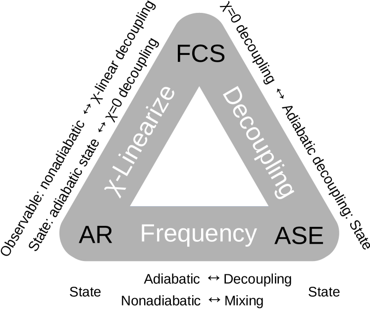
Figure 5: Relations between adiabatic-state evolution (ASE, Appendix G), adiabatic-response (AR, Sec. III) and full-counting statistics (FCS, Sec. V) approach discussed in the text.

“Adiabatic” FCS solution.

The “adiabatic” solution of the FCS master equation (101) can be written using Eq. (108), (114) and (115) as

$${|{\rho^{\chi,\text{i}}(t)})} =e^{i\chi\left[\Delta X^{r,\text{i}}(t)+\Delta X^{r,\text{a}}(t)\right]+\ldots}\Big{[}{|{\rho^{\text{i}}[{\mathbf{R}}(t)]})}+\ldots\Big{]}$$ (140)

Here only the $\chi$-linear terms are indicated since we exclusively discuss the first moment. A $\chi$-linear term in the eigenvector [Eq. (126b)] is also omitted since it is redundant [zero trace, cf. Eq. (94)]. From hereon we will not indicate such omissions ($\ldots$) for clarity.

$\chi=0$: FCS is adiabatic. In this case, the “adiabatic” FCS generating operator (140) only keeps track of the adiabatic, zeroth order in frequency, result for the state:

$$\left.{|{\rho^{\chi,\text{i}}(t)})}\vphantom{I^{I^{I}}}\right|_{\chi=0}={|{\rho^{\text{i}}[{\mathbf{R}}(t)]})}.$$ (141)

Thus, only that part of the AR [Eq. (97)] and ASE [Eq. (215a)] result is kept that describes the instantaneous dependence on the driving parameters. Here the label “i” is thus appropriate.

$\chi\neq 0$: FCS is nonadiabatic. In contrast, the generating operator ${|{\rho^{\chi,\text{i}}(t)})}$ for nonzero $\chi$ is not a function of the instantaneous parameters alone. By introducing $\chi$, the FCS circumvents the normalization constraint that prevents a Berry-Simon phase from appearing in the AR and ASE approach for the steady-state (cf. Sec. III.1). The FCS gauge freedom (132a) for $\chi\neq 0$ allows the exponential term in Eq. (140) to accumulate a dependence on parameters at all previous times $t^{\prime}\in[t,0]$. We found [Eq. (127)-(128)] that at $t=\mathcal{T}$ this produces the sum of the dynamical term $\Delta X^{r,\text{i}}=\int_{0}^{\mathcal{T}}dt^{\prime}I_{X^{r}}^{\text{i}}[{\mathbf{R}}(t^{\prime})]$ and the geometric term $\Delta X^{r,\text{a}}=\int_{0}^{\mathcal{T}}dt^{\prime}I_{X^{r}}^{\text{a}}[{\mathbf{R}}(t^{\prime})]=\oint_{\mathcal{C}}dRA_{0}[{\mathbf{R}}]$ as given by the AR expressions (46) and (48), respectively ($g=0$ gauge). As in the original Berry-Simon situation, the geometric term ($\propto(\dot{{\mathbf{R}}})^{1}$) in the exponent is of one order higher in the driving frequency than the dynamical one ($\propto(\dot{{\mathbf{R}}})^{0}$, c.f. Eq. (49) and Appendix G). In this way, the FCS also includes the pumped observable of nonadiabatic origin by allowing the “adiabatic” solution (140) to accumulate a phase.

Remarkably, this is an effect of the nonadiabatic state correction $\rho^{\text{a}}$, that we have just neglected in the $\chi=0$ part [Eq. (141)]. How does the FCS keep track of this effect without calculating $\rho^{\text{a}}$ explicitly? A reconsideration of our perturbative treatment of the $\chi$-linearization $W^{\chi}=W+i\chi W_{\hat{I}_{X^{r}}}$ sheds some light on how this is achieved by combining the $\chi$-bookkeeping with “adiabatic” decoupling. As in Sec. V.3.1 this requires us to consider currents and the FCS master equation (101). We now think for a moment of Eq. (140) as a solution ansatz, ${|{\rho^{\chi,\text{i}}(t)})}=e^{i\chi\Delta X^{r}(t)}{|{\rho^{\text{i}}[{\mathbf{R}}(t)]})}$, in which the transported observable $\Delta X^{r}(t)$ is to be determined. One notes that the nonredundant part of right eigenvector, ${|{\rho^{\text{i}}[{\mathbf{R}}(t)]})}$, from which it is built contains no nonadiabatic information whatsoever. Neither does the corresponding eigenvalue: it is just the instantaneous current, $\lambda_{0}^{\chi}[{\mathbf{R}}(t)]=i\chi I_{X^{r}}^{\text{i}}[{\mathbf{R}}(t)]$. The nonadiabatic effect can thus only enter through the step of “adiabatic” decoupling, i.e, when inserting this ansatz into the FCS master equation $\frac{d}{dt}{|{\rho^{\chi}})}=W^{\chi}{|{\rho^{\chi}})}$ and projecting this onto the eigenspace with the corresponding left eigenvector ${({\bar{v}^{\chi}_{0}}|}={({\mathbbm{1}}|}-i\chi{({\Phi_{X^{r}}}|}$. One immediately obtains an equation for the nonadiabatic part of the total FCS current $\tfrac{d}{dt}\Delta X^{r}(t)$:

$$I_{X^{r}}^{\text{a}}:=[\tfrac{d}{dt}\Delta X^{r}(t)]-I_{X^{r}}^{\text{i}}={({\Phi_{X^{r}}}|}\tfrac{d}{dt}{|{\rho^{\text{i}}})}.$$ (142)

This shows most directly that by the formal “adiabatic” decoupling, the instantaneous state ${|{\rho^{\text{i}}})}$ is combined with a time-derivative and the nonadiabatic response covector ${({\Phi_{X^{r}}}|}$. Only together they produce the nonadiabatic effect for observable $\hat{X}^{r}$. Even though the AR expression $\rho^{\text{a}}=W^{-1}\tfrac{d}{dt}{|{\rho^{\text{i}}})}$ does not explicitly appear, the FCS thus keeps track of the three required pieces required on the right hand side of Eq. (142) in three different places.

The response covector has precisely the right form ${({\Phi_{X^{r}}}|}={({\mathds{1}}|}W_{\hat{I}_{X^{r}}}W^{-1}$ [Eq. (126c)] required to obtain the AR result by a perturbative mixing. This is the point, where the physical “lag” enters the FCS analysis [cf. the AR discussion of Eq. (79)]. The formal $\chi$-controlled mixing of ${({\mathbbm{1}}|}$ with ${({\Phi_{X^{r}}}|}$ into the left eigenvector thus substitutes for the nonadiabatic coupling induced by physical time evolution. It is this mixing that allows the FCS to circumvent the probability normalization obstructing geometric phase accumulation (Sec. III.1).

Finally, we also note how the gauge transformation in the FCS corresponds to the physical meter-recalibration $X^{r}\to X^{r}_{g}=X^{r}+g\mathbbm{1}$, discussed in the AR approach [Eq. (63b) ff.]. One obtains the same generating operator when changing the gauge factor of the right eigenvector while compensating for this by using $X^{r}_{g}$ instead of $X^{r}$ in the ansatz ${|{\rho^{\chi,\text{i}}(t)})}=e^{i\chi\Delta X^{r}_{g}(t)}\cdot\big{[}e^{-i\chi[g[{\mathbf{R}}(t)]-g[{\mathbf{R}}(0)]]}{|{\rho^{\text{i}}[{\mathbf{R}}(t)]})}\big{]}$. The “adiabatic” decoupling then leads to a different FCS current,

$$I_{X^{r}_{g}}^{\text{a}}:=[\tfrac{d}{dt}\Delta X^{r}_{g}(t)]-I_{X^{r}}^{\text{i}}={({\Phi_{X^{r}}}|}\tfrac{d}{dt}{|{\rho^{\text{i}}})}+\tfrac{d}{dt}g$$ (143)

which, however, integrates to the correct value $\Delta X^{r,\text{a}}$.

“Nonadiabatic” corrections to FCS.

We now address the question whether or not the slow driving required for the “adiabaticity” of the FCS implies that it should neglect nonadiabatic effects it produces. It is therefore relevant to compare the terms that the approaches in Fig. 5 neglect. These conditions have received little attention in FCS works that compute the first moment of pumping, see however LABEL:Sinitsyn07EPL.

For this we return to the general formulation of the FCS of Sec. V.1 and decompose the generating operator as follows:

$$\rho^{\chi}=\rho^{\chi,\text{i}}+\rho^{\chi,\text{a}}+{\rho}^{\chi,\text{rest}}.$$ (144)

As noted before, this labeling is tentative and we should distinguish zero and nonzero values of $\chi$.

$\chi=0$: FCS neglects nonadiabatic effects. In this case each term reduces by Eq. (97) to the corresponding contribution in the ASE and AR expansion:

$$\rho=\rho^{\text{i}}+\rho^{\text{a}}+{\rho}^{\text{rest}}.$$ (145)

For $\chi=0$ the labeling is thus appropriate. For the FCS to be consistent, the nonadiabatic correction plus higher corrections that are neglected must be small relative to the “adiabatic” one that is kept:

$$||\rho^{\text{rest}}+\rho^{\text{a}}||\ll||\rho^{\text{i}}||.$$ (146)

This condition is satisfied if the condition (51) of slow driving, $|\dot{{\mathbf{R}}}|\ll\Gamma$, holds, since it guarantees $||\rho^{\text{rest}}||\ll||\rho^{\text{a}}||\ll||\rho^{\text{i}}||$. This can equivalently be expressed as a gap condition commonly used to justify the decoupling of eigenspaces [Eq. (212)]. For the ASE approach this leads to the same driving restriction as for the AR approach [Eq. (213)]. A possible source of confusion is that in the AR approach the contribution $\rho^{\text{a}}$ is necessarily and correctly kept, being aware that it is small [Eq. (50)].

$\chi\neq 0$: FCS keeps leading nonadiabatic effects, neglecting higher ones. In the FCS approach consistency also requires that the moments computed by Eq. (88) with $t_{0}\rightarrow 0$ from the “adiabatic” solution dominate the ones that are neglected, i.e., the first “nonadiabatic” correction and higher ones:

$$\partial_{i\chi}^{n}{({\mathbbm{1}|\rho^{\chi,\text{rest}}+\rho^{\chi,\text{a}}})}|_{\chi=0}\ll\partial_{i\chi}^{n}{({\mathbbm{1}|\rho^{\chi,\text{i}}})}|_{\chi=0}.$$ (147)

For the first moment, $n=1$, noting on the right hand side that the FCS result reduces to the AR expressions [Eq. (127)-(128)], we obtain

$$|\Delta X^{r,\text{rest}}|\ll|\Delta X^{r,\text{i}}+\Delta X^{r,\text{a}}|.$$ (148)

Both terms on the left in Eq. (147) together form the term on the left in Eq. (148), while the term on the right in Eq. (147) produces both terms on the right in Eq. (148). Here the tentative labeling is thus not appropriate but as mentioned above this is unavoidable. Importantly, the consistency condition Eq. (148) is exactly that of the AR approach [Eq. (53)], in which the small $\rho^{\text{a}}$ is kept to compute $\Delta X^{r,\text{a}}$. Thus, within the FCS this nonadiabatic effect is effectively kept, despite the fact that one neglects “nonadiabatic” effects in the state based on a gap condition at $\chi=0$.

As summarized in Fig. 5, in the FCS approach “adiabaticity” is merely a formal statement about the validity of the decoupling similar to the ASE, but applied to a formal device, the generating operator $\rho^{\chi}$. In contrast, in the AR approach (non)adiabaticity is directly related to different terms in a frequency expansion, corresponding to the (corrections to) decoupling of eigenspace in the ASE approach in the steady-state limit. This underlines that the useful notions of “adiabaticity”, “Berry-Simon phase” and “decoupling” should carefully be distinguished, in particular in open quantum systems with a unique stationary state. Our discussion illustrates the usefulness of having a clear physical picture of what all the geometric notions in a problem with gauge freedom stand for, going beyond the level of “the final result can be written as a curve integral”.

V.4 Discussion of the FCS approach

Having answered question (iv) of Sec. II.5 regarding the equivalence of the FCS and AR approach, we emphasize the obvious advantage of the FCS approach when one actually goes beyond the first moment of pumped quantities on which we focused here, as, e.g., in Refs. Ren and Sinitsyn, 2013; Li et al., 2014. As discussed from its inception Levitov and Lesovik (1993), the FCS can be considered a full description of an ideal meter detecting transport of an observable, see also LABEL:Schaller09. The relation between meter recalibrations and gauge freedom in pumping formalisms, highlighted in our paper in the simplest setting, deserves further consideration within the more general FCS approach, possibly, also for non-ideal meters.

However, in applications where FCS is used only to calculate the first moment it must be stressed that a definite overhead is introduced: besides deriving a more complicated kernel $W^{\chi}$, one needs to compute a specific instantaneous eigenvalue of $W^{\chi}$ with both its left and right eigenvectors in dependence of the continuous variable $\chi$. Even when one afterwards linearizes in $\chi$ to extract only the first moment, this is much more involved than solving the corresponding problem analytically or numerically in the AR approach, even for very simple models. For more complicated systems, the FCS approach may become so involved that in order to make progress, one may be inclined to introduce further approximations, which are unnecessary when using the AR approach. As explicitly shown here and in LABEL:Nakajima15, $\chi$-linearizing FCS calculations before hand amounts to using the AR approach. This overhead is even more relevant when considering strong coupling and memory effects [Eq. (11)-(12)] on geometric pumping that arise beyond the Born-Markov approximation Splettstoesser et al. (2006, 2010).

VI Discussion and outlook

In this paper, we have discussed the geometric nature of pumping through open quantum systems using the reduced density-operator approach. We focused explicitly on the memoryless, weak-coupling, high-temperature limit and the ubiquitous case of a unique parametric stationary state. This allows treating geometric pumping phases of complicated discrete quantum systems with essentially arbitrary local interactions, including in particular geometric phases that, in order to emerge, require interactions.

We outlined how in our solution of the physical pumping problem (much simpler than equivalent alternative approaches) a local gauge freedom emerges in the relation between a measured pumped observable (two-point expectation value) and an observable operator [Eq. (59)]: the choice of gauge corresponds to a meter calibration. In striking contrast to closed quantum systems, the gauge freedom is therefore a nonunitary group, reflecting the very different physical setting in which geometry enters here: the observable, not the quantum-state, accumulates the geometric phase over one driving period, as physically expected in transport problems.

Our paper combines definite computational advantages with a clear view of the tangible physical meaning of all relevant geometric concepts. We tie together the differential geometry defined by a connection $A_{X^{r}_{g}}$ with non-adiabaticity [$\dot{{\mathbf{R}}}(t)$] and the gauge freedom of recalibrations: the Landsberg geometric connection is essentially the nonadiabatic part of the current

$$A_{X^{r}_{g}}[{\mathbf{R}}(t)]=\frac{\delta I_{X^{r}_{g}}({\mathbf{R}},\dot{{\mathbf{R}}}(t))}{\delta\dot{{\mathbf{R}}}(t)},$$ (149)

with $X^{r}_{g}=X^{r}+g\mathds{1}$. The corresponding curvature of this connection, its curl, is the pumped charge per unit area of the driving-parameter space. We provided explicit formulas for the efficient computation of pumping phases applicable to very general interacting systems that are weakly coupled to reservoirs, showing how computational overhead can be avoided and conservation laws, present for specific observables, can be exploited. We demonstrated these advantages for the example of a single-level Anderson quantum dot illustrating how a geometric pumping phase can be induced by electron-electron interaction.

Moreover, we showed that the geometric “horizontal lift” defined by this connection corresponds to a (discontinuous) meter gauge that maintains the physical pumping current $I_{X^{r}_{g}}^{\text{a}}$ to be zero at each time instant by continuously adjusting the scale to follow the meter’s “needle.” The geometric-phase “jump” (the holonomy) exhibited by this horizontal lift is given by the resulting cumulative adjustment of the meter’s scale over a driving period, i.e., the pumped observable per period. We believe this is the most direct geometric significance one can attach to physical transport quantities in a pumping experiment. We demonstrated the importance of such a clear view by discussing the important issue how “adiabatic” approximations employed in the full-counting-statistics (FCS) approach produces a (correct) geometric pumping phase that is due to nonadiabatic currents.

It is an interesting question as to whether and how our approach relates to ideas for closed systems, in particular to the widely used Berry-Simon formulation of geometric phases appropriate for quantum state evolution. Such a relation can be established, but requires a construction different from –but relying on– the one presented in this paper and will be discussed elsewhere Wegewijs et al. . In fact, aside from the obvious consideration of topological pumping effects in strongly interacting systems, our work can be continued in several other directions:

(i) An important implication of our work is that Landsberg’s geometric framework is compatible with the more general adiabatic-response approach to pumping based on real-time kernels Splettstoesser et al. (2006) [Eq. (11)]: the nonuniqueness in the choice of the observable operator during a driving cycle does not rely on the state dynamics. We thus expect that the present approach can be extended to non-Markovian, strongly-coupled open quantum systems with a unique parametric stationary state. For this reason, we stressed that the gauge structure already requires attention when deriving quantum master equations and expectation value of the current for a nonsystem observable, an issue that has received little to no attention so far. This is crucial since measurements that display geometric effects are performed in the environment, that one would like to integrate out to keep the calculations simple. These are situations which existing formulations, such as generalizations of Kato’s method to open systemsAvron et al. (2012b), have not dealt with.

(ii) Our paper stressed the important distinction between the gauge freedom of the quantum state and that of the pumped observable. We showed that the state gauge freedom is quenched in the ubiquitous case of a unique stationary state for fixed driving parameters, our well-motivated working assumption. Clearly, an interesting extension of our work would be to consider nonunique stationary states Avron et al. (2012a) leading to an interplay of the state gauge freedom with the independent observable gauge freedom in steady-state pumping. Counter to standard intuition, a two-fold degenerate stationary state does not yet lead to a non-Abelian gauge freedom, but to an Abelian one due to physical restrictions imposed by trace and Hermiticity preservation, which are often not discussed. For higher degeneracies of the stationary state, a non-Abelian gauge structure does seem to emerge, but this requires a careful account of the mentioned nontrivial restrictions.

(iii) One may furthermore also consider a more complicated gauge group of non-Abelian character for the observable. In fact, Landsberg’s general geometric framework has already been extended to this case in LABEL:AnderssonThesis,Andersson05. However, its relation to the physical density operator formalism and to measurable pumping quantities (the starting point stressed throughout this paper) needs to be clarified first.

In any case, to address these important problems, the present formulation of Landsberg’s approach seems to provide the simplest and physically most transparent geometric picture: for the simple, but ubiquitous, class of problems addressed here, we demonstrated this by explicit comparison with several other approaches, highlighting geometric, physical and computational advantages. Our work illustrates that the standard intuition about geometric effects in quantum physics needs to be drastically reconsidered when turning to open quantum systems and motivates further work into this direction.

Appendix A Born kernels and conservation law

In this section we derive the Born-approximation to the kernels governing the dynamics of the system state [Eq. (24)] and the expectation values of nonsystem observables [(30)]. We also derive the simplification (83) in case the observable is conserved at a junction.

Partial normal ordering. Although we follow the well-known Wangsness-Bloch approach Koller et al. (2010), a key point, central to the issue of gauge freedom addressed in the main text, deserves to be highlighted: it is crucial to split up both the coupling $V$ and the nonsystem observables $\hat{X}^{r}$ into a partially averaged term and a partially normal-ordered term according to Eq. (29).

Throughout the paper it is assumed that the coupling $V(t)$ is partially normal ordered, i.e.,

$${\langle{V(t)}\rangle}^{\text{res}}=0.$$ (150)

This constitutes no approximation since for any Hamiltonian of the form of Eq. (13) the coupling can be partially normal ordered by absorbing the partial average of the original coupling, which is a system operator, into the system Hamiltonian.

Assuming initial decoupling of system and reservoir state, i.e., $\rho^{\text{tot}}(0)=\rho\otimes\rho^{\text{res}}$, and the interaction picture

$$A_{I}\coloneqq e^{i(H+H^{\text{res}})t}Ae^{-i(H+H^{\text{res}})t}$$ (151)

the Liouville-von Neumann differential equation for the total system state reads as

$$\partial_{t}{\rho}^{\text{tot}}_{I}(t) =-i\left[V_{I}(t),{\rho}^{\text{tot}}_{I}(t)\right]$$ (152a)

$${\rho}^{\text{tot}}_{I}(t_{0}) =\rho_{I}(t_{0})\otimes{\rho}^{\text{res}},$$ (152b)

which is equivalent to the Dyson integral equation

$${\rho}^{\text{tot}}_{I}(t)={\rho}^{\text{tot}}_{I}(t_{0})-i\int_{t_{0}}^{t}dt^{\prime}\left[V_{I}(t^{\prime}),{\rho}^{\text{tot}}_{I}(t^{\prime})\right].$$ (153)

Time-evolution kernel. To obtain the evolution equation for the reduced density operator $\rho_{I}(t)=\underset{\text{res}}{\mathsf{Tr}}{\rho}^{\text{tot}}_{I}(t)$ to leading order $V^{2}\sim\Gamma$ in the coupling, we insert Eq. (153) into Eq. (152a) and take the partial trace

$$\partial_{t}\rho_{I}(t)= -i\underset{\text{res}}{\mathsf{Tr}}\Big{[}V_{I}(t),{\rho}^{\text{tot}}_{I}(t_{0})\Big{]}$$

$$-\int_{t_{0}}^{t}dt^{\prime}\underset{\text{res}}{\mathsf{Tr}}\Big{[}V_{I}(t),\Big{[}V_{I}(t^{\prime}),{\rho}^{\text{tot}}_{I}(t^{\prime})\Big{]}\Big{]}.$$ (154)

The first term in Eq. (154) vanishes due to the partial normal-ordering (150). The second term in Eq. (154) can be simplified consistent with the Born approximation by inserting

$${\rho}^{\text{tot}}_{I}(t^{\prime})\approx\rho_{I}(t^{\prime})\otimes{\rho}^{\text{res}}$$ (155)

since the corrections, computed in LABEL:Koller10, end up in higher orders of the kernel, which we neglect. As a result, within the Born-approximation the kinetic equation reads in the interaction-picture

$$\partial_{t}\rho_{I}(t)=-\int_{t_{0}}^{t}dt^{\prime}\underset{\text{res}}{\mathsf{Tr}}\Big{[}V_{I}(t),\Big{[}V_{I}(t^{\prime}),\rho_{I}(t^{\prime}){\rho}^{\text{res}}\Big{]}\Big{]}$$ (156)

and, correspondingly, in the Schrödinger picture

$$\partial_{t}\rho(t)=-i\left[H,\rho(t)\right]+\int_{t_{0}}^{t}W(t-t^{\prime})\rho(t^{\prime})$$ (157)

with the time-nonlocal kernel Eq. (24) of the main text:

$$W(t-t^{\prime})\bullet=$$ (158)

$$-\underset{\text{res}}{\mathsf{Tr}}\left[V,e^{-i\left[H+{H}^{\text{res}}\right](t-t^{\prime})}\left[V,{\rho}^{\text{res}}\bullet\right]e^{+i\left[H+{H}^{\text{res}}\right](t-t^{\prime})}\right].$$

Observable kernels. For an arbitrary time-dependent nonsystem observable we can proceed in close analogy. The crucial step is not to approximate the expectation value of $\hat{X}^{r}_{I}(t)$, but instead the expectation value of its partially normal-ordered part [Eq. (29)],

$${\langle{\mathop{:}\nolimits\!\hat{X}^{r}(t)\!\mathop{:}\nolimits}\rangle} ={\langle{\hat{X}^{r}(t)}\rangle}-\mathsf{Tr}\left({\langle{\hat{X}^{r}(t)}\rangle}^{\text{res}}\rho_{I}(t)\right),$$ (159)

which does not exhibit fluctuations in the sense that

$${\langle{\mathop{:}\nolimits\!\hat{X}^{r}(t_{0})\!\mathop{:}\nolimits}\rangle}^{\text{res}}=0.$$ (160)

Now, inserting the Dyson equation (153) into the expectation value we obtain two terms, similar to Eq. (154):

$${\langle{\mathop{:}\nolimits\!\hat{X}^{r}(t)\!\mathop{:}\nolimits}\rangle}= \mathsf{Tr}\underset{\text{res}}{\mathsf{Tr}}\mathop{:}\nolimits\!\hat{X}^{r}_{I}(t)\!\mathop{:}\nolimits{\rho}^{\text{tot}}_{I}(t)$$ (161a)

$$= \mathsf{Tr}\underset{\text{res}}{\mathsf{Tr}}\mathop{:}\nolimits\!\hat{X}^{r}_{I}(t)\!\mathop{:}\nolimits{\rho}^{\text{tot}}_{I}(t_{0})$$ (161b)

$$-i\mathsf{Tr}\int_{t_{0}}^{t}dt^{\prime}\underset{\text{res}}{\mathsf{Tr}}\hat{X}^{r}_{I}(t)\left[V_{I}(t^{\prime}),{\rho}^{\text{tot}}_{I}(t^{\prime})\right].$$ (161c)

Again, the first term (161b) vanishes by virtue of partial normal ordering of the observable: inserting the initially factorizing state (152b) and using Eq. (160)

$$\mathsf{Tr}\underset{\text{res}}{\mathsf{Tr}}\mathop{:}\nolimits\!\hat{X}^{r}_{I}(t_{0})\!\mathop{:}\nolimits{\rho}^{\text{tot}}_{I}(t_{0})=\mathsf{Tr}{\langle{\mathop{:}\nolimits\!\hat{X}^{r}_{I}(t_{0})\!\mathop{:}\nolimits}\rangle}^{\text{res}}\rho_{I}(t_{0})=0.$$ (162)

In the second term (161c) we again insert the Born approximation (155). In analogy to Eq. (156) we thus obtain

$${\langle{\mathop{:}\nolimits\!\hat{X}^{r}(t)\!\mathop{:}\nolimits}\rangle}$$ (163a)

$$=-i\mathsf{Tr}\int_{t_{0}}^{t}dt^{\prime}\underset{\text{res}}{\mathsf{Tr}}\mathop{:}\nolimits\!\hat{X}^{r}_{I}(t)\!\mathop{:}\nolimits\Big{[}V_{I}(t^{\prime}),\rho_{I}(t^{\prime}){\rho}^{\text{res}}\Big{]}$$ (163b)

$$=-i\mathsf{Tr}\int_{t_{0}}^{t}dt^{\prime}\underset{\text{res}}{\mathsf{Tr}}\tfrac{1}{2}\Big{[}\mathop{:}\nolimits\!\hat{X}^{r}_{I}(t)\!\mathop{:}\nolimits,\Big{[}V_{I}(t^{\prime}),\rho_{I}(t^{\prime}){\rho}^{\text{res}}\Big{]}\Big{]}_{+}.$$ (163c)

In the last step to Eq. (163c) we have used that for a product $AB=\tfrac{1}{2}[A,B]+\tfrac{1}{2}[A,B]_{+}$ the commutator part does not contribute under the trace. As mentioned after Eq. (67), this is equivalent to changing $W_{\mathop{:}\nolimits\!X\!\mathop{:}\nolimits}\to W_{\mathop{:}\nolimits\!X\!\mathop{:}\nolimits}+\Theta$ by a superoperator with $\mathsf{Tr}\,\Theta\,\bullet=0$. Using Eq. (159) we obtain the expectation value (27) of the main text:

$${\langle{\hat{X}^{r}(t)}\rangle}=\mathsf{Tr}{\langle{\hat{X}^{r}(t)}\rangle}^{\text{res}}\rho(t)+\mathsf{Tr}\int_{t_{0}}^{t}dt^{\prime}W_{\mathop{:}\nolimits\!X^{r}\!\mathop{:}\nolimits}(t,t^{\prime})\rho(t^{\prime}),$$ (164)

with the time-nonlocal observable kernel (30)

$$W_{\mathop{:}\nolimits\!X^{r}\!\mathop{:}\nolimits}(t,t^{\prime})\bullet=-i\tfrac{1}{2}\times$$ (165)

$$\underset{R}{\mathsf{Tr}}\left[\mathop{:}\nolimits\!\hat{X}^{r}(t)\!\mathop{:}\nolimits\,,e^{-i\left[H+{H}^{\text{res}}\right](t-t^{\prime})}\left[V,{\rho}^{\text{res}}\bullet\right]e^{+i\left[H+{H}^{\text{res}}\right](t-t^{\prime})}\right]_{+},$$

which explicitly depends only on the partially normal-ordered part of the observable $\mathop{:}\nolimits\!\hat{X}^{r}\!\mathop{:}\nolimits$.

Conservation law at a junction $r$. We now derive the identity (83), which is used to simplify Eq. (30), assuming that the ${\mathbf{R}}$-independent nonsystem observable $\hat{X}^{r}$´ is conserved as in Eq. (81). We follow LABEL:Saptsov12a [Eq. (174) ff.] adapting the simpler formulation used in the above derivations. We allow the system operator $\hat{X}[{\mathbf{R}}]$ to depend on ${\mathbf{R}}$ (cf. Sec. IV).

Accounting for our assumptions that $\hat{X}^{r}$ is ${\mathbf{R}}$-independent, $[\hat{H}^{r},\hat{X}^{r}]=0$ [Eq. (35)] and $[\hat{H},\hat{X}]=0$ [Eq. (82)], the current operators read as

$$\hat{I}_{X^{r}}=i[V^{r},\hat{X}^{r}],\qquad\hat{I}_{X}=i\sum_{r}[V^{r},\hat{X}]+\frac{\partial\hat{X}}{\partial t}.$$ (166)

The conservation law (81) implies that the part of the current due to the coupling $V^{r}$, indicated by $|_{r}$, is conserved:

$${\langle{\hat{I}_{X^{r}}}\rangle} ={\langle{i[V^{r},\hat{X}^{r}]}\rangle}$$ (167)

$$=-{\langle{i[V^{r},\hat{X}]}\rangle}:=-{\langle{\hat{I}_{X}-\tfrac{\partial\hat{X}}{\partial t}}\rangle}|_{r}.$$ (168)

Going to the interaction picture, the right hand side is easily related to the state evolution:

$${\langle{\hat{I}_{X}-\tfrac{\partial\hat{X}}{\partial t}}\rangle}|_{r}$$ (169a)

$$=-i\mathsf{Tr}\underset{\text{res}}{\mathsf{Tr}}\,[\hat{X}_{I}(t),V^{r}_{I}(t)]{\rho}^{\text{tot}}_{I}(t)$$ (169b)

$$=\mathsf{Tr}\hat{X}_{I}(t)\underset{\text{res}}{\mathsf{Tr}}\Big{\{}-i[V^{r}_{I}(t),{\rho}^{\text{tot}}_{I}(t)]\Big{\}}$$ (169c)

$$=-\mathsf{Tr}\hat{X}_{I}(t)\int_{t_{0}}^{t}dt^{\prime}\underset{\text{res}}{\mathsf{Tr}}\left[V_{I}^{r}(t),\left[V_{I}(t^{\prime}),\rho_{I}(t^{\prime}){\rho}^{\text{res}}\right]\right].$$ (169d)

In step (169b) we used $\mathsf{Tr}\mathsf{Tr}_{\text{res}}[A,B]C=\mathsf{Tr}\mathsf{Tr}_{\text{res}}A[B,C]$ to pull the leftmost system operator out of the reservoir trace. Under the partial trace in Eq. (169c) we have precisely the right hand side of the Liouville equation (152a) except for $V_{I}(t)\to V^{r}_{I}(t)$ and we thus perform the same steps that led from Eq. (154) to Eq. (156)].

In the resulting Eq. (169d), the time-integral is just the right hand side of the kinetic equation (156) “resolved with respect to junction-$r$” at the latest time $t$. Correspondingly, in the Schrödinger picture we obtain

$${\langle{\hat{I}_{X^{r}}}\rangle}(t) =-\mathsf{Tr}\hat{X}(t)\int_{t_{0}}^{t}dt^{\prime}W^{r}(t,t^{\prime})\rho(t^{\prime})$$ (170)

where $W^{r}(t,t^{\prime})$ is obtained from Eq. (158) by simply replacing $V(t)\to V^{r}(t)$. Finally, by comparing the Markov limit of Eq. (164) for $\hat{X}^{r}\to\hat{I}_{X^{r}}$ and the Markov limit of Eq. (170) we obtain the result (83) of the main text

$${\langle{\hat{I}_{X^{r}}}\rangle}(t) =\mathsf{Tr}W_{\hat{I}_{X^{r}}}(t)\rho(t)=-\mathsf{Tr}\hat{X}W^{r}\rho(t)$$ (171)

with $W_{\hat{I}_{X^{r}}}:=W_{\mathop{:}\nolimits\!I_{X^{r}}\!\mathop{:}\nolimits}(t)+{\langle{\hat{I}_{X^{r}}}\rangle}^{\text{res}}$ defined as in Eq. (41).

Appendix B Conservation law - example

Here we illustrate how Eq. (83) in the main text takes a more commonly known form when it is expressed in terms of “current rates” as in LABEL:Schoeller97hab. For the stationary-state charge current into the reservoir $r$:

$$I_{N^{r}}={({\mathbbm{1}}|}W_{\hat{I}_{N^{r}}}{|{\rho^{\text{i}}})}=-{({N}|}W^{r}{|{\rho^{\text{i}}})}.$$ (172)

Let $|k\rangle$ be a particle-number eigenstate, i.e., $\hat{N}=\sum_{k}N_{k}|k\rangle\langle k|$ with particle number $N_{k}$ in state $k$. We now expand the density operator in basis operators ${|{kk^{\prime}})}:=|k\rangle\langle k^{\prime}|$ and expand ${({N}|}\bullet=\mathsf{Tr}\hat{N}\bullet=\sum_{j}N_{j}{({jj}|}$ in the dual basis ${({jj^{\prime}}|}=\mathsf{Tr}|j^{\prime}\rangle\langle j|$. For simplicity we ignore contributions from the off-diagonal elements $k\neq k^{\prime}$ of the stationary-state density operator in the $H$-basis. Denoting the transition rates ${({jj}|}W^{r}{|{kk})}:=W^{r}_{j,k}$ we obtain the well-known expression

$$I_{N^{r}} =-\sum_{k}\sum_{j}N_{j}W^{r}_{jk}\rho^{\text{i}}_{kk}+\ldots$$ (173)

$$=-\sum_{k}\sum_{j\neq k}\left(N_{j}-N_{k}\right)W^{r}_{j,k}\rho^{\text{i}}_{kk}+\ldots,$$ (174)

using only the probability conservation $W_{kk}^{r}=-\sum_{j\neq k}W_{j,k}^{r}$. Physically, this counts minus the change in $N$ going from state $k\to j$, which by conservation of $\hat{N}+\hat{N}^{r}$ should equal the change in $\hat{N}^{r}$.

Appendix C Pumping vs. instantaneous contribution

Here, we discuss how the different scalings with parameters, mentioned in Sec. II.4, allow the instantaneous part (46) and adiabatic-response part (47) and (48) to be separately extracted from measurements, both in principle and in practice. How can one get rid of the nongeometric “sum of snapshots” of the instantaneous current, even in strong nonequilibrium situations? In particular, one would like to do this directly in an experiment  in view of applications where pumping current is the main tool (Sec. I), but also in view of the pumping spectroscopy discussed in Sec. IV.2. We summarize three possible ways to extract the geometric pumped charge from the instantaneous background:

(a) Zero bias: $I_{X^{r}}^{\text{i}}(t)=\Delta X^{r,\text{i}}=0$. The characteristic of this case of pure pumping is that although at each instant the current for $\hat{X}^{r}$ is zero, a cyclic parameter change can still transport this observable.

(b) Bias driving with cancellations: $I_{X^{r}}^{\text{i}}(t)\neq 0$ but $\Delta X^{r,\text{i}}=0$. When driving the applied bias the instantaneous current is generally nonzero. The “sum of snapshots” may, however, still average to zero if the bias-driving probes regions with opposing currents. This happens, e.g., for charge transport through a symmetrically coupled quantum dot when driving gate and bias voltage at constant frequency $\Omega$.

If this cancellation is slightly incomplete for constant frequency, e.g., due to a nonsymmetric coupling, then one may slowly modulate the frequency to shift weight between positive and negative contributions during the period in order to still achieve cancellation and realize $\Delta X^{r,\text{i}}=0$. Importantly, this does not alter the adiabatic-response part because of its geometric nature: it depends only on the traversed parameter curve.

Another possibility is to perform a global modulation of the coupling, i.e., a time-dependent, spatially uniform rescaling of all couplings by $V^{r}[{\mathbf{R}}]\to\sqrt{\alpha[{\mathbf{R}}]}V^{r}[{\mathbf{R}}]$ with a nonnegative function $\alpha[{\mathbf{R}}]$. Such a rescaling modifies the instantaneous current by $I_{X^{r}}^{\text{i}}\to\alpha I_{X^{r}}^{\text{i}}$ but drops out in the pumping current: $I_{X^{r}}^{\text{a}}\to I_{X^{r}}^{\text{a}}$. This modification of the instantaneous part can be used to cancel it to zero by equally weighting forward and backward instantaneous current contributions along the driving cycle. Then, after one driving cycle only a geometric pumped charge remains.

(c) General case with bias and/or bias driving: $I_{X^{r}}^{\text{i}}(t)\neq 0$ and $\Delta X^{r,\text{i}}\neq 0$. Finally, if the driving cycle probes only parameter values with a definite bias, then one is “pumping with / against the flow” and the cancellation cannot be achieved in the way indicated above. However, a simple modification of the measurement scheme as suggested in LABEL:Sinitsyn07PRB still allows one to cancel out the instantaneous part: one first drives the system for a large number of cycles $M$ and measures the total observable during time $M\mathcal{T}$. One then reverses the time-dependent driving protocol and repeats the measurement. Subtracting the two measurements and dividing by $2M$ the instantaneous part cancels out (it does not change sign), leaving only the pumping part.

Situation (a) is at the focus of studies motivated by metrology Jehl et al. (2013), where topological protection is desired. Here, its geometric nature protects the pumping signal against various kinds of perturbations of the driving protocol. For example, different parametrizations ${\mathbf{R}}(t)$ of the same curve, e.g., due to fluctuations in the driving speed, leave the pumping invariant. Also, the deformation of the driving cycle has a smaller effect on the pumping contribution than on the stationary part since the former scales with the area enclosed by the driving cycle for small amplitude driving.

Situations (b)-(c) are relevant to recent studies discussing pumping Ren et al. (2010); Nakajima et al. (2015), pumping-spectroscopy Calvo et al. (2012); Reckermann et al. (2010); Haupt et al. (2013); Riwar et al. (2013), and excess entropy production in nonequilibrium thermodynamics Yuge et al. (2013) in the presence of a nonlinear bias. The interesting point here is that the pumping contribution contains spectroscopic information Splettstoesser et al. (2006) that is not contained in the averaged stationary-state information of in the instantaneous part.

Appendix D Interaction-induced pumping through a quantum dot

Here we explicitly work out the AR approach for the simple fermionic example of electron charge pumping through a single orbital quantum dot. This example was analyzed in LABEL:Calvo12a. Here we extend it by allowing for driving of the tunnel barrier and in fact of any parameter. This serves as an illustration of the general approach presented in this paper.

The system Hamiltonian describing such an example reads as

$$H=\epsilon N+BS_{z}+\tfrac{1}{2}N_{\uparrow}N_{\downarrow}U.$$ (175)

with bilinear tunnel couplings $V^{r}$ specified through tunnel rates $\Gamma_{r}$ (treated in the wide-band limit) and electron reservoirs $r=\text{L, R}$, characterized by $T$ and $\mu^{r}$. The magnetic field $B$ is initially added for our comparison with the FCS approach in Appendix I. We later focus on zero magnetic field results Refs. Reckermann et al., 2010; Calvo et al., 2012; Yoshii and Hayakawa, 2013; Nakajima et al., 2015, and make use of the supplementary information to LABEL:Schulenborg16a where more details can be found.

State dynamics. We first give the time-evolution kernel in Eq. (25)). Due to spin and charge conservation the off-diagonal elements of the quantum-dot density operator $\rho$ in the $H$-eigenbasis, describing, e.g., the transverse spin $S_{x}$ and $S_{y}$, decouple from the diagonal ones describing the spin $S_{z}$ along $B$ and the charge ($N$) dynamics. We can thus restrict the state dynamics to Liouville vectors spanned by pure states for an empty, spin-up, spin-down- and double occupied quantum dot, respectively:

$${|{\rho})}=p_{0}|0\rangle\langle 0|+\sum_{\sigma}p_{\sigma}|\sigma\rangle\langle\sigma|+p_{2}|2\rangle\langle 2|.$$ (176)

Acting on this subspace, the Liouvillian $L[{\mathbf{R}}]$ that we defined into the effective $W[{\mathbf{R}}]$ in Eq. (26) is zero and can thus be ignored. In this basis the master equation (25) for the example of this section reads

$$\partial_{t}\begin{pmatrix}p_{0}\\ p_{\uparrow}\\ p_{\downarrow}\\ p_{2}\end{pmatrix}=\begin{pmatrix}-W_{\uparrow,0}-W_{\downarrow,0}&W_{0,\uparrow}&W_{0,\downarrow}&0\\ W_{\uparrow,0}&-W_{0,\uparrow}-W_{2,\uparrow}&0&W_{\uparrow,2}\\ W_{\downarrow,0}&0&-W_{0,\downarrow}-W_{2,\downarrow}&W_{\downarrow,2}\\ 0&W_{2,\uparrow}&W_{2,\downarrow}&-W_{\uparrow,2}-W_{\downarrow,2}\end{pmatrix}\begin{pmatrix}p_{0}\\ p_{\uparrow}\\ p_{\downarrow}\\ p_{2}\end{pmatrix}.$$ (177)

Letting $\bar{\sigma}$ denote the opposite of $\sigma=\uparrow,\downarrow$ and $\epsilon_{\sigma}=\epsilon+\sigma B/2$, the rates $W_{x,y}=\sum_{r}W^{r}_{x,y}$ are given by

$$W^{r}_{\sigma,0} =\Gamma_{r}f^{+}_{r}(\epsilon_{\sigma}), W^{r}_{2,\overline{\sigma}} =\Gamma_{r}f^{+}_{r}(\epsilon_{\sigma}+U),$$

$$W^{r}_{0,\sigma} =\Gamma_{r}f^{-}_{r}(\epsilon_{\sigma}), W^{r}_{\overline{\sigma},2} =\Gamma_{r}f^{-}_{r}(\epsilon_{\sigma}+U),$$ (178)

with the Fermi functions $f^{\alpha}_{r}(\omega)=1/(1+\exp\alpha(\omega-\mu_{r})/T)$ and temperature $T$.

Now focusing on the case of zero magnetic field, $B=0$, the charge dynamics decouples from spin $S_{z}$ as well. Changing the operator basis for $N=1$ to the mixed spin state $\tfrac{1}{2}\sum_{\sigma}|\sigma\rangle\langle\sigma|$ and the spin-operator $\tfrac{1}{2}\sum_{\sigma}\sigma|\sigma\rangle\langle\sigma|=S_{z}$ and defining transition rates

$$W^{r}_{1,0} =\Gamma_{r}f^{+}_{r}(\epsilon) W^{r}_{2,1} =2\Gamma_{r}f^{+}_{r}(\epsilon+U)$$

$$W^{r}_{0,1} =2\Gamma_{r}f^{-}_{r}(\epsilon) W^{r}_{1,2} =\Gamma_{r}f^{-}_{r}(\epsilon+U)$$ (179)

we obtain the master equation reduced to charge subspace:

$$\partial_{t}\begin{pmatrix}p_{0}\\ p_{1}\\ p_{2}\end{pmatrix}=\begin{pmatrix}-W_{1,0}&W_{0,1}&0\\ W_{1,0}&-W_{0,1}-W_{2,1}&W_{1,2}\\ 0&W_{2,1}&-W_{1,2}\end{pmatrix}\begin{pmatrix}p_{0}\\ p_{1}\\ p_{2}\end{pmatrix}.$$ (180)

Here $p_{N}$ is the occupation probability of the charge $N=0,1,2$ state, which is a mixed state for $N=1$ and a pure one for $N\neq 1$.

We now introduce the time-dependent driving through any of the parameters entering the master equation via Eq. (179). There is little need to explicitly express the rates $W_{N,N^{\prime}}$ in terms of ${\mathbf{R}}$. We only illustrate for this example how to define these dimensionless parameters, required in the main text, starting from the physical quantities $\epsilon,\mu^{\text{L}},\mu^{\text{R}},U,\Gamma^{\text{L}},\Gamma^{\text{R}}$. Since $\epsilon,\mu^{\text{L}},\mu^{\text{R}},U$ enter the master equation through Fermi functions in Eq. (179), temperature $T$ is a relevant energy scale. The tunnel strengths $\Gamma^{\text{L}},\Gamma^{\text{R}}$ play a special role since they set the scale of the rates in Eq. (179), in contrast to the other parameters. The time-average of the total tunnel strengths $\bar{\Gamma}=\bar{\Gamma}^{\text{L}}+\bar{\Gamma}^{\text{R}}$ can be used to normalize them. Note that both the scales $T$ and $\bar{\Gamma}$ are by our assumptions nonnegative. Thus, the driving parameters can be concretely chosen as

$${\mathbf{R}}=\left(\frac{\epsilon}{T},\frac{\mu^{\text{L}}-\mu^{\text{R}}}{T},\frac{U}{T},\frac{\Gamma^{\text{L}}}{\bar{\Gamma}},\frac{\Gamma^{\text{R}}}{\bar{\Gamma}}\right).$$ (181)

Using the notation of Sec. V.3.2 the real eigenvalues, left and right eigenvectors of the superoperator $W$ in Eq. (180) are

Eigenvalue Left eigenvector Right eigenvector

$$\lambda_{0}=0 {\overline{v}_{0}}=\scalebox{0.8}{\mbox{$\displaystyle\begin{pmatrix}1&1&1\end{pmatrix}$}} {v_{0}}=\scalebox{0.8}{\mbox{$\displaystyle\frac{1}{\frac{W_{0,1}}{W_{1,0}}+\frac{W_{2,1}}{W_{1,2}}+1}\begin{pmatrix}\frac{W_{0,1}}{W_{1,0}}\\ 1\\ \frac{W_{2,1}}{W_{1,2}}\end{pmatrix}$}}$$ (182a)

$$\lambda_{1}=-\frac{1}{2}(W_{1,0}+W_{1,2}) {\overline{v}_{1}}=\scalebox{0.8}{\mbox{$\displaystyle\begin{pmatrix}-\frac{W_{1,0}}{W_{0,1}-W_{2,1}}&1&\frac{W_{1,2}}{W_{0,1}-W_{2,1}}\end{pmatrix}$}} {v_{1}}=\scalebox{0.8}{\mbox{$\displaystyle\scalebox{0.9}{\mbox{$\displaystyle\frac{1}{\frac{W_{1,0}W_{0,1}+W_{1,2}W_{2,1}}{(W_{0,1}-W_{2,1})^{2}}+1}$}}\begin{pmatrix}-\frac{W_{0,1}}{W_{0,1}-W_{2,1}}\\ 1\\ \frac{W_{2,1}}{W_{0,1}-W_{2,1}}\end{pmatrix}$}}$$ (182b)

$$\lambda_{2}=-W_{1,0}-2W_{0,1}=-2\Gamma {\overline{v}_{2}}=\scalebox{0.8}{\mbox{$\displaystyle\begin{pmatrix}\frac{W_{1,0}}{W_{0,1}}&-2&\frac{W_{1,2}}{W_{2,1}}\end{pmatrix}$}} {v_{2}}=\scalebox{0.8}{\mbox{$\displaystyle\frac{1}{\frac{W_{1,0}}{W_{0,1}}+\frac{W_{1,2}}{W_{2,1}}+4}\begin{pmatrix}1\\ -2\\ 1\end{pmatrix}$}}$$ (182c)

where the parameter dependence has been suppressed. The zero eigenvalue $\lambda_{0}$ is associated with preservation of the trace, represented by ${({\bar{v}_{0}}|}$, and with the unique stationary state ${|{v_{0}})}={|{\rho^{\text{i}}})}$. The negative eigenvalues $\propto\Gamma$ describe the decay mode of the charge $\hat{N}$, ${|{v_{1}})}$, and fermion-parity Contreras-Pulido et al. (2012); Saptsov and Wegewijs (2012, 2014) $(-\mathbbm{1})^{\hat{N}}$, ${|{v_{2}})}$, and their associated amplitude covectors. These are additionally required to compute the response vector.

Observable response vector. We focus on charge pumping and choose for the observable operator

$$X^{r}=N^{r}.$$ (183)

As mentioned in the main text [Eq. (57)] and discussed in LABEL:Calvo12a, at this point we already make use of the gauge freedom $N^{r}\to N^{r}+g[{\mathbf{R}}]\mathbbm{1}$: to compute the physical time-dependent currents in a quantum dot one actually needs to account for screening currents Bruder and Schoeller (1994). The resulting screening currents average out in one driving period. Thus, the gauge freedom in the observable is used from the start to discard these, Eq. (183) giving the correct pumped charge.

Since charge is conserved by the tunnel coupling, i.e., $[V^{r},N+N^{r}]=0$ [Eq. (81)], we can use the simplification (83) to obtain the connection (73a). With the pseudo inverse $W^{-1}=\sum_{k=1,2}\tfrac{1}{\lambda_{k}}{|{v_{k}})}{({\overline{v}_{k}}|}$ and using

$$2W^{r}_{0,1}[{\mathbf{R}}]+W^{r}_{1,0}[{\mathbf{R}}] =2\Gamma^{r}[{\mathbf{R}}]$$ (184)

$$2W^{r}_{2,1}[{\mathbf{R}}]+W^{r}_{1,2}[{\mathbf{R}}] =2\Gamma^{r}[{\mathbf{R}}]$$ (185)

using notation borrowed from LABEL:Schulenborg16a the pumping response-covector Eq. (84) is obtained as:

$${({\Phi_{N^{r}}[{\mathbf{R}}]}|} =-{({\hat{N}}|}W^{r}[{\mathbf{R}}]\frac{1}{W[{\mathbf{R}}]}$$ (186a)

$$=\frac{\lambda_{1}^{r}[{\mathbf{R}}]}{\lambda_{1}[{\mathbf{R}}]}\,\left[{({\hat{N}}|}-N_{0}[{\mathbf{R}}]\,{({\mathbbm{1}}|}\right]$$ (186b)

$$\propto{({\overline{v}_{1}[{\mathbf{R}}]}|}\,,$$ (186c)

where $N_{0}[{\mathbf{R}}]={({N|v_{0}[{\mathbf{R}}]})}$ is the frozen-parameter stationary-state charge. Since ${({\mathds{1}|{\mathbf{\nabla_{R}}}\rho^{i}[{\mathbf{R}}]})}=0$ the ${\mathbf{R}}$-dependence responsible for charge pumping enters only through the first nonzero eigenvalue of $W^{r}$

$$\lambda_{1}^{r}[{\mathbf{R}}]=-\tfrac{1}{2}\big{[}W^{r}_{1,0}[{\mathbf{R}}]+W^{r}_{1,2}[{\mathbf{R}}]\big{]}$$ (187)

and the eigenvalue $\lambda_{1}=\sum_{r}\lambda_{1}^{r}$ of $W$. The reason that the other eigenvalues $\lambda_{2}$ and $\lambda_{2}^{r}$ of $W$ and $W^{r}$, respectively, do not contribute is that the eigenvector ${|{v_{2}})}\propto{|{v_{2}^{r}})}\propto(-1)^{N}$ is the fermion parity operator which plays a special role Schulenborg et al. (2016).

Pumping connection and curvature. Combining Eq. (182a) with Eq. (186) we obtain for the charge-pumping connection (73a)

$$A_{0}[{\mathbf{R}}]={({\Phi_{N^{r}}|{\mathbf{\nabla_{R}}}\rho^{\text{i}}})}=$$ (188a)

$$\frac{\lambda_{1}^{r}[{\mathbf{R}}]}{2\lambda_{1}^{3}[{\mathbf{R}}]}\Big{[}W_{1,0}[{\mathbf{R}}]{\mathbf{\nabla_{R}}}W_{1,2}[{\mathbf{R}}]-W_{1,2}[{\mathbf{R}}]{\mathbf{\nabla_{R}}}W_{1,0}[{\mathbf{R}}]\Big{]}$$ (188b)

and for the pumping curvature (85)

$$B[{\mathbf{R}}]={({{\mathbf{\nabla_{R}}}\Phi_{N^{r}}}|}\times{|{{\mathbf{\nabla_{R}}}\rho^{\text{i}}})}=$$ (189)

$$=\frac{\lambda_{1}^{r}[{\mathbf{R}}]}{\lambda_{1}^{3}[{\mathbf{R}}]}{\mathbf{\nabla_{R}}}W_{1,0}[{\mathbf{R}}]\times{\mathbf{\nabla_{R}}}W_{1,2}[{\mathbf{R}}] +{\mathbf{\nabla_{R}}}\Big{[}\frac{\lambda_{1}^{r}[{\mathbf{R}}]}{2\lambda_{1}^{3}[{\mathbf{R}}]}\Big{]}\times\Big{[}W_{1,0}[{\mathbf{R}}]{\mathbf{\nabla_{R}}}W_{1,2}[{\mathbf{R}}]-W_{1,2}[{\mathbf{R}}]{\mathbf{\nabla_{R}}}W_{1,0}[{\mathbf{R}}]\Big{]}.$$ (190)

This result illustrates the geometric spectroscopy of Sec. IV: when driving the system energies $H$ relative to the reservoirs $\mu^{r}$ for fixed coupling parameters $\Gamma^{r}$, both ${({{\mathbf{\nabla_{R}}}\Phi_{N^{r}}}|}$ and ${|{{\mathbf{\nabla_{R}}}\rho^{\text{i}}})}$ show sharp changes. Due to the different functional dependence of covector and vector, their gradients are nonparallel, i.e., Eq. (80) is violated and a pumping response can be expected at sharply defined parameter points. Similar considerations hold for, e.g., the gradients ${\mathbf{\nabla_{R}}}W_{1,N}$ for $N=0,2$ in Eq. (189).

In the present case, this pumping effect is induced by the interaction Reckermann et al. (2010); Calvo et al. (2012); Haupt et al. (2013) $U$ if the tunnel rates are not driven. That the curvature vanishes in this case, can be seen from both formulas. First, setting $U=0$ in the pumping curvature Eq. (190) we find

$${\mathbf{\nabla_{R}}}W_{1,0}[{\mathbf{R}}]+{\mathbf{\nabla_{R}}}W_{1,2}[{\mathbf{R}}]={\mathbf{\nabla_{R}}}\Gamma[{\mathbf{R}}]$$ (191)

$$\lambda_{1}^{r}[{\mathbf{R}}]=-\Gamma^{r}[{\mathbf{R}}],\quad\lambda_{1}[{\mathbf{R}}]=-\Gamma[{\mathbf{R}}].$$ (192)

where we used $f^{+}_{r}+f^{-}_{r}=1$ in Eq. (179). For constant tunnel strengths the gradients ${\mathbf{\nabla_{R}}}W_{1,0}$ and ${\mathbf{\nabla_{R}}}W_{1,2}$ are (anti)parallel vectors, making the first term vanish, even though the parameter dependence of rates for electron and hole processes is different. In the second term in Eq. (190), the first gradient is zero.

If one only wants to see that the curvature vanishes it is easier to use Eq. (189) and first set $U=0$. In this case, the form (186b) of the response covector is simple because the $N_{0}$ part drops out in the connection

$$A_{0}[{\mathbf{R}}]=\frac{\lambda_{1}^{r}[{\mathbf{R}}]}{2\lambda_{1}^{3}[{\mathbf{R}}]}{({N|{\mathbf{\nabla_{R}}}\rho^{\text{i}}[{\mathbf{R}}]})}.$$ (193)

by probability conservation, ${({\mathds{1}|{\mathbf{\nabla_{R}}}\rho^{i}[{\mathbf{R}}]})}=0$. Thus the only relevant part of the response covector is parameter independent if the tunnel strengths are constant and hence the pumping curvature vanishes [Eq. (79) ff.]. This advantage of this derivation allows to avoid the evaluation of ${\mathbf{\nabla_{R}}}\rho^{\text{i}}$ in Eq. (186c). We note that to compute nonzero curvature values for $U\neq 0$ the explicit form (190) is more convenient.

We therefore find that pumping without driving the tunnel rates is interaction induced, i.e., there is no pumping effect in the absence of interaction, i.e., if $U=0$ during the whole driving cycle. This does not depend on the driving protocol or the choice of parameters, as long as the tunnel rates and interaction stay constant. We note that when driving the interaction $U$ itself, a pumping contribution can still arise as parameter regions with nonzero interaction are visited during the driving cycle.

The second curvature contribution in Eq. (190) was not given in LABEL:Reckermann10a,Calvo12a,Haupt13 since the tunnel rates were assumed to be constant from the start. If this is not the case, driving of tunnel rates may result in pumping even without interaction. Similar interaction-induced pumping effects have been discussed in different contextsSinitsyn and Nemenman (2007a); Ren et al. (2010).

Appendix E Pumping of system observables -
AR approach of Avron, et. al Avron et al. (2012a)

In this appendix we show how the AR approach of Avron, Fraas, and Graf, in LABEL:Avron12 fits into our considerations of gauge freedom of observables in Sec. III when we replace nonsystem observable $\hat{X}^{r}$ by a system observable $\hat{X}[{\mathbf{R}}]$. We extend their considerations by allowing for possible parametric time-dependence of the observable including that introduced by a gauge transformation.

The Heisenberg current superoperator for a gauged system observable $\hat{X}_{g}(t):=\hat{X}[{\mathbf{R}}(t)]+g[{\mathbf{R}}(t)]\mathbbm{1}$ reads when written under the trace ${({\mathbbm{1}}|}=\mathsf{Tr}$

$${({\mathbbm{1}}|}W_{\hat{I}_{X_{g}}}[{\mathbf{R}}(t)]={({X}|}W[{\mathbf{R}}(t)]+\frac{d}{dt}g[{\mathbf{R}}(t)]{({\mathbbm{1}}|}.$$ (194)

In this simpler situation of a system observable, this can be directly seen: following LABEL:Avron12, the right hand side of Eq. (194) is calculated by inserting $\frac{d}{dt}\rho(t)=W(t)\rho(t)$ into the expectation value $\frac{d}{dt}{\langle{\hat{X}_{g}}\rangle}(t)=\frac{d}{dt}{({\hat{X}_{g}|\rho(t)})}={({\mathbbm{1}}|}W_{\hat{I}_{X_{g}}}{|{\rho(t)})}$. This is the system-observable analog to the Heisenberg equation of motion (41) for nonsystem observables where $W[{\mathbf{R}}]$ is effectively replaced by $W^{r}[{\mathbf{R}}]$. Here, it is not necessary to start from the total system current (55) as we did in deriving the current kernel (41). Note, in particular, that in the above we did not assume that $\left[H,X\right]=0$, as we did in Eq. (82).

As in LABEL:Avron12, we now solve the master equation for the adiabatic response, $\rho^{\text{a}}=\frac{1}{W}{\mathbf{\nabla_{R}}}\rho^{\text{i}}$, and obtain for the transported observable $\Delta X=\Delta X^{\text{i}}+\Delta X^{\text{a}}$:

$$\Delta X^{\text{i}} =\int_{0}^{\mathcal{T}}dt{({\mathbbm{1}}|}W_{\hat{I}_{X}}[{\mathbf{R}}(t)]{|{\rho^{\text{i}}[{\mathbf{R}}(t)]})}$$ (195)

$$\Delta X^{\text{a}} =\int_{\mathcal{C}}d{\mathbf{R}}A_{g}[{\mathbf{R}}]=\int_{\mathcal{S}}dSB[{\mathbf{R}}]$$ (196)

where we recognize the Landsberg connection $A_{g}[{\mathbf{R}}]=A_{0}[{\mathbf{R}}]+{\mathbf{\nabla_{R}}}g[{\mathbf{R}}]$ with

$$A_{0}[{\mathbf{R}}] ={({X[{\mathbf{R}}]}|}Q[{\mathbf{R}}]{|{{\mathbf{\nabla_{R}}}\rho^{\text{i}}[{\mathbf{R}}]})}.$$ (197)

As in LABEL:Avron12 the result is expressed in the non-Hermitian projector on the Liouville subspace complementary to the unique stationary-state zero eigenvalue on which the pseudo-inverse $W^{-1}$ is computed:

$$Q[{\mathbf{R}}]:=W[{\mathbf{R}}]\frac{1}{W[{\mathbf{R}}]}=\mathcal{I}-{|{\rho^{\text{i}}[{\mathbf{R}}]})}{({\mathbbm{1}}|}$$ (198)

Our derivation emphasizes that the projector $Q$ has two factors: $W$ comes from the system observable [Eq. (194)], whereas $W^{-1}$ accounts of the “lag” time of the evolution [Eq. (79) ff.]. The pumping connection (197) corresponds to Theorem 9 of LABEL:Avron12. We refer to this work for a detailed discussion, as well as additional interesting results which find no parallel in the present paper, e.g., the case of nonunique stationary states. The corresponding curvature

$$B[{\mathbf{R}}] ={({X[{\mathbf{R}}]}|}\Big{[}{\mathbf{\nabla_{R}}}Q[{\mathbf{R}}]\Big{]}\times{|{{\mathbf{\nabla_{R}}}\rho^{\text{i}}[{\mathbf{R}}]})}$$ (199a)

$$+{({{\mathbf{\nabla_{R}}}X[{\mathbf{R}}]}|}\,Q[{\mathbf{R}}]\times{|{{\mathbf{\nabla_{R}}}\rho^{\text{i}}[{\mathbf{R}}]})}.$$ (199b)

shows that the ${\mathbf{R}}$-dependence of projector $Q$ in the term (199a) generates pumping as shown in LABEL:Avron12 [cf. our discussion in Sec. IV of conserved nonsystem observables Eq. (84)]. The term (199b) does not appear in LABEL:Avron12 since there $\hat{X}$ is explicitly assumed to be ${\mathbf{R}}$ independent, but it is related to our discussion following Eq. (82).

The geometric pumping response of LABEL:Avron12, there formulated elegantly in terms Liouville-space Kato projections, can thus also be considered as another instance of Landsberg’s nonadiabatic geometric phase. The gauge freedom responsible for the geometric effect lies in the observable and the relevant fiber bundle is the same as that discussed in Figs. 1 - 4 with $\hat{X}^{r}\to\hat{X}$. Our discussion of LABEL:Avron12 thus underscores a number of key points of of the main text in a simpler setting:

(i) Pumping involves a geometric nonadiabatic response of the quantum state relative to the instantaneous solution of the Berry-Robbins type (“geometric magnetism”) Berry and Robbins (1993).

(ii) Although geometric, the pumping effect is not a “Berry-Simon” phase, i.e., associated with adiabatic state evolution: the gauge freedom responsible for the result Eq. (197) lies in the observable, not in the state.

(iii) The connection Eq. (197) relies critically on the decay to a unique frozen-parameter stationary state, a key feature distinguishing Landsberg’s phase in dissipative systems from the Berry-Simon phase.

(iv) From Sec. V it is now also clear that the results of an FCS approach for pumping of the first moment of system observables will reduce to those obtained by the simpler AR approach of LABEL:Avron12.

Appendix F Response covector – Generalized Brouwer formula.

In LABEL:Calvo12a, pumping-response coefficients were introduced that are closely related to our response covector (79) (see also LABEL:Avron12). These allow to bring the Landsberg curvature (78) into a form similar to the well-known Brouwer formula Brouwer (1998) valid in the noninteracting / mean-field picture of transport. Additional terms arise for conserved parameter-dependent system observables. In the presence of interactions, model-specific calculations Splettstoesser et al. (2006, 2008); Reckermann et al. (2010); Calvo et al. (2012); Riwar et al. (2013) have been shown to take such a form. Here we briefly describe how the considerations of LABEL:Calvo12a extend to our more general setting.

To obtain the Brouwer-type form, one expands the instantaneous stationary state $\rho^{\text{i}}$ in any complete orthonormal basis of observables $\hat{Y}[{\mathbf{R}}]=\hat{Y}^{\dagger}[{\mathbf{R}}]$, i.e., for which $\sum_{Y}{|{Y[{\mathbf{R}}]})}{({Y[{\mathbf{R}}]}|}=\mathcal{I}$ with ${|{Y[{\mathbf{R}}]})}=\hat{Y}[{\mathbf{R}}]$, ${({Y[{\mathbf{R}}]}|}\bullet=\mathsf{Tr}\,\hat{Y}[{\mathbf{R}}]\bullet$. For example, for an interacting, single-orbital quantum dot coupled to normal metal electrodes, one possible set of such observables is $\{\hat{Y}\}=\{\mathbbm{1},\hat{N},\hat{S}_{z},(-\mathbbm{1})^{\hat{N}}\}$. In the expansion

$${|{\rho^{\text{i}}[{\mathbf{R}}]})}=\sum_{Y}{|{Y[{\mathbf{R}}]})}\,{\langle{Y}\rangle}^{\text{i}}[{\mathbf{R}}].$$ (200)

the coefficients are the stationary-state averages of these observables, ${\langle{\hat{Y}}\rangle}^{\text{i}}[{\mathbf{R}}]={({Y[{\mathbf{R}}]|\rho^{\text{i}}[{\mathbf{R}}]})}=\mathsf{Tr}\,\hat{Y}[{\mathbf{R}}]\rho^{\text{i}}[{\mathbf{R}}]$. In Brouwers formula, the pumping response of reservoir-observable $\hat{X}^{r}$ is expressed in terms of the responses of the averages of these system observables. In our case, using Eq. (78) the pumping curvature with the expansion (200) is

$$B_{X^{r}}[{\mathbf{R}}]=\sum_{Y} {({{\mathbf{\nabla_{R}}}\Phi_{X^{r}}[{\mathbf{R}}]|Y[{\mathbf{R}}]})}\times{\mathbf{\nabla_{R}}}{\langle{\hat{Y}}\rangle}^{\text{i}}[{\mathbf{R}}]$$

$$+ {({{\mathbf{\nabla_{R}}}\Phi_{X^{r}}[{\mathbf{R}}]}|}\times{|{{\mathbf{\nabla_{R}}}Y[{\mathbf{R}}]})}\ {\langle{\hat{Y}}\rangle}^{\text{i}}[{\mathbf{R}}].$$ (201)

The first term in Eq. (201) is similar to Brouwer’s formula. It contains the parameter gradient of the average system observables, whereas in the second term these averages appear by themselves. Moreover in the first term the role of response vector (79) is to assign to each system observable $\hat{Y}[{\mathbf{R}}]$ its response-coefficient ${({\Phi_{X^{r}}[{\mathbf{R}}]|Y[{\mathbf{R}}]})}=\mathsf{Tr}\,\Phi_{X^{r}}^{\dagger}[{\mathbf{R}}]\hat{Y}[{\mathbf{R}}]$ under the ${\mathbf{\nabla_{R}}}$ in Eq. (201). Although similar to Brouwer’s formula, Eq. (201) holds for strongly interacting, weakly coupled open quantum systems, with (possibly nonconserved) nonsystem observable $\hat{X}^{r}$.

Without further assumptions, there is no natural choice for the $\{\hat{Y}[{\mathbf{R}}]\}$: unitary transformations of this basis of operators leave (201) invariant. This nonuniqueness may seem a disadvantage that Eq. (201) as compared to the basis-independent response-covector Eq. (79). However, when $\hat{X}^{r}+\hat{X}[{\mathbf{R}}]$ is conserved at junction $r$ [Eq. (81)] we can exploit the simplification (84) by including the corresponding system observable $\hat{X}[{\mathbf{R}}]$ in the expansion set $\{\hat{Y}[{\mathbf{R}}]\}$. The pumping-response of the conserved observable $\hat{X}^{r}$ can then be written as a “self-response” plus cross-responses of other, linearly independent observables $\hat{Y}[{\mathbf{R}}]$:

$$B_{X^{r}}[{\mathbf{R}}]=$$ (202)

$$-\Big{[}{\mathbf{\nabla_{R}}}{({X[{\mathbf{R}}]}|}W^{r}[{\mathbf{R}}]\frac{1}{W[{\mathbf{R}}]}\Big{]}{|{X})}\times{\mathbf{\nabla_{R}}}{\langle{\hat{X}[{\mathbf{R}}]}\rangle}^{\text{i}}-\Big{[}{\mathbf{\nabla_{R}}}{({X[{\mathbf{R}}]}|}W^{r}[{\mathbf{R}}]\frac{1}{W[{\mathbf{R}}]}\Big{]}\times{|{{\mathbf{\nabla_{R}}}X[{\mathbf{R}}]})}\ {\langle{\hat{X}[{\mathbf{R}}]}\rangle}^{\text{i}}$$

$$-\sum_{Y\neq X}\left\{\Big{[}{\mathbf{\nabla_{R}}}{({X[{\mathbf{R}}]}|}W^{r}[{\mathbf{R}}]\frac{1}{W[{\mathbf{R}}]}\Big{]}{|{Y})}\times{\mathbf{\nabla_{R}}}{\langle{\hat{Y}[{\mathbf{R}}]}\rangle}^{\text{i}}-\Big{[}{\mathbf{\nabla_{R}}}{({X[{\mathbf{R}}]}|}W^{r}[{\mathbf{R}}]\frac{1}{W[{\mathbf{R}}]}\Big{]}\times{|{{\mathbf{\nabla_{R}}}Y[{\mathbf{R}}]})}\ {\langle{\hat{Y}[{\mathbf{R}}]}\rangle}^{\text{i}}\right\}$$

For example, for charge pumping, with parameter independent $X$ and $Y$, in LABEL:Splettstoesser06 only the first term played a role ($\hat{X}=\hat{N}$) due to spin-symmetry, whereas in LABEL:Reckermann10a the cross-talk with the spin ($\hat{Y}=\hat{S}_{z}$) in the third term is relevant as well. In Refs. Calvo et al., 2012; Haupt et al., 2013 spin pumping also involved two terms ($\hat{X}=\hat{S}_{z}$ and $\hat{Y}=\hat{N}$). Importantly, Eq. (202) also applies to discrete many-particle systems whose stationary state is specified by a larger set of observables.

Appendix G Adiabatic geometric phase for mixed states:
ASE approach of Sarandy and Lidar

In the main text we make repeated use of insights offered by the ASE approach of Refs. Sarandy and Lidar, 2005, 2006, an approach not related to pumping. Here we summarize the required key points, but also discuss some relevant issues that can not be found in Refs. Sarandy and Lidar, 2005, 2006.

Adiabatic approximation. Sarandy and Lidar consider a time-local master equation for the density operator

$$\frac{d}{dt}{|{\rho(t)})}=W(t){|{\rho(t)})}.$$ (203)

Since this approach can deal with non-steady-state evolution it is convenient to start the evolution from state $\rho(0)$ at $t_{0}=0$ (instead of $t_{0}\to-\infty$ as in the main text). In our setting, we assume the kernel decomposes as

$$W(t)=\sum_{n}\lambda_{n}(t){|{v_{n}(t)})}{({\overline{v}_{n}(t)}|}$$ (204)

with the right- and left eigenvectors ${|{v_{n}(t)})}$ and ${({\overline{v}_{n}(t)}|}$ to the possibly complex eigenvalues $\lambda_{n}(t)$. The eigenvalues are assumed to be nondegenerate for simplicity and to have non-positive real parts. The density operator is expanded in the right eigenvectors

$${|{\rho})}(t)=\sum_{n}e^{\Lambda_{n}(t)}\rho_{n}(t){|{v_{n}(t)})},$$ (205)

where the anticipated dynamical “phase” $\Lambda_{n}(t)=\int_{0}^{t}dt^{\prime}\lambda_{n}(t^{\prime})$ is split off right away. Inserting this ansatz into Eq. (203) yields coupled equations for the coefficients:

$$\partial_{t}\rho_{n}(t)= -{({\overline{v}_{n}(t)|\partial_{t}v_{n}(t)})}\rho_{n}(t)$$ (206)

$$-\sum_{m\neq n}{({\overline{v}_{n}(t)|\partial_{t}v_{m}(t)})}\rho_{m}(t)e^{\Lambda_{m}(t)-\Lambda_{n}(t)}.$$

At this point we apply the adiabatic approximation for open quantum systems, discussed carefully by Sarandy and Lidar Sarandy and Lidar (2005), which amounts to neglecting the second line in Eq. (206). The condition under which this is valid is described in Eq. (212). The adiabatic approximation, here labeled by “i” for “instanteneous” as in the main text, for the non-steady-state solution of the master-equation (203) is given by:

$${|{\rho^{\text{i}}(t)})}=\sum_{n}e^{\Lambda_{n}(t)}e^{\gamma_{n}(t)}\rho_{n}(0){|{v_{n}(t)})}.$$ (207)

Thus, in the adiabatic evolution the components of the mixed state ${|{\rho(t)})}$ in the various different instantaneous eigenspaces of $W(t)$ evolve independently of each other. Each eigenvector ${|{v_{n}(t)})}$ evolves with its own geometric phase factor determined by a separate connection for each eigenspace $n$:

$$\gamma_{n}(\mathcal{T})=-\oint_{\mathcal{C}}d{\mathbf{R}}A_{n}[{\mathbf{R}}]$$ (208)

$$A_{n}[{\mathbf{R}}]:={({\overline{v}_{n}[{\mathbf{R}}]|\partial v_{n}[{\mathbf{R}}]})}.$$ (209)

This is the most direct generalization of the Berry-Simon phase for adiabatic time evolution to open systems evolving with Eq. (203).

Adiabatic-response correction. In LABEL:Sarandy05 the first nonadiabatic correction to the result Eq. (207), here labeled “a” for “adiabatic-response” as in the main text, is shown to be

$${|{\rho^{\text{a}}(t)})}= \sum_{n}{|{v_{n}(t)})}\left\{\sum_{m\neq n}e^{\Lambda_{m}(t)}e^{\gamma_{m}(t)}\frac{{({\overline{v}_{n}(t)|\partial_{t}v_{m}(t)})}}{\lambda_{n}(t)-\lambda_{m}(t)}\rho_{m}(0)-\sum_{m\neq n}e^{\Lambda_{n}(t)}e^{\gamma_{n}(t)}\frac{{({\overline{v}_{n}(0)|\partial_{t}v_{m}(0)})}}{\lambda_{n}(0)-\lambda_{m}(0)}\rho_{m}(0)\right.$$

$$\left.+\sum_{m\neq n}e^{\Lambda_{n}(t)}e^{\gamma_{n}(t)}\int_{0}^{t}d\tau\frac{{({\overline{v}_{n}(\tau)|\partial_{\tau}v_{m}(\tau)})}{({\overline{v}_{m}(\tau)|\partial_{\tau}v_{n}(\tau)})}}{\lambda_{n}(\tau)-\lambda_{m}(\tau)}\rho_{n}(0)\right\}.$$ (210)

Both lines of (210) each can be understood in an intuitive picture. The first line describes processes where an initial state $m$ “leaks” into state $n$ via the coupling term

$$\tfrac{{({\overline{v}_{n}(\tau)|\partial_{\tau}v_{m}(\tau)})}}{\lambda_{n}(\tau)-\lambda_{m}(\tau)}$$ (211)

either at final time $\tau=t$ or initial time $\tau=0$. The “phase” factors (exponentials) correspond to the dynamics after and before the transition. The second term can be understood as a leakage from the state $n$ into itself: it contains the coupling terms for a transition from $n$ to $m$ and back. Although this seems to be a higher order contribution, it is in fact not since one integrates such processes over all possible times.

Gap condition. Reference LABEL:Sarandy05 derives the gap condition ensuring the validity of the adiabatic decoupling, i.e., neglecting the correction (210) relative to the adiabatic solution (207), similar to the closed system case, as

$$\max_{0<t<\mathcal{T}}\,\,\left|\frac{{({\overline{v}_{n}(t)|\partial_{t}v_{m}(t)})}}{\lambda_{n}(t)-\lambda_{m}(t)}\right|\,\ll\,||\bar{v}_{n}||\,||v_{m}||.$$ (212)

for all $n$,$m$. For a system driven at frequency $\Omega$ with dimensionless amplitudes $\delta{\mathbf{R}}$ and eigenvalues with relevant scale $\Gamma$ the condition (212) gives:

$$\Big{|}\frac{\delta{\mathbf{R}}\Omega}{\Gamma}\Big{|}\ll 1.$$ (213)

This is identical to Eq. (51) of the main text. It is crucial to note the distinct ways in which this gap condition is used:

(a) In both the ASE and the FCS approaches, this is the condition to neglect the adiabatic response ${|{\rho^{a}})}$ or ${|{\rho^{\chi,\text{a}}})}$.

(b) In the AR approach, at the focus of the main text, this condition is used to justify [Appendix H] keeping the adiabatic-response, yet neglecting higher adiabatic corrections (nonlinear in $\Omega$), which scale with $(\delta{\mathbf{R}}{\Omega}/{\Gamma})^{2}$.

We stress this point here and in in the main text since it easily leads to confusion. For example, in Sec. V.3.4 we show that in the FCS the kept “adiabatic” / ”instantaneous” contribution, through the “$\chi$-bookkeeping-device” of the FCS, in fact leads back to case (b): one effectively uses Eq. (213) to motivate keeping a physically nonadiabatic (!) part.

Gauge freedom in adiabatic mixed-state evolution. Similar to the closed-system case, the non-degenerate instantaneous eigenvectors of the kernel $W(t)$ are only determined up to a nonzero complex time-dependent factor, which is, however, complex: a gauge transformation with $c_{n}(t)\in\mathds{C}/\{0\}$, preserving the biorthonormality,

$${|{v_{n}(t)})} \rightarrow\,c_{n}(t)\,{|{v_{n}(t)})}$$ (214a)

$${({\overline{v}_{n}(t)}|} \rightarrow c^{-1}_{n}(t){({\overline{v}_{n}(t)}|}$$ (214b)

clearly leaves the kernel $W(t)$ invariant and thus also the solution of the master equation (203) remains unchanged. In agreement with this, the density operator contributions (207) and (210) are invariant under gauge transformations: although, the connections (209) are gauge dependent, transforming as $A_{n}\to A_{n}+c_{n}^{-1}{\mathbf{\nabla_{R}}}c_{n}$, these enter only through the invariant geometric phases (208).

In our discussion of the Landsberg (Sec. III) and the FCS (Sec. V) approaches we made use of the following important result which was not discussed in Refs. Sarandy and Lidar, 2005, 2006: the gauge freedom (214) still contains a mathematical redundancy which can be eliminated by taking into account two physical restrictions on the evolution of the mixed-state $\rho(t)$.

(a) First, the preservation of the trace-normalization of $\rho(t)$, i.e., $0=\partial_{t}\mathsf{Tr}{{\rho}}={({\mathds{1}|W|\rho})}$, requires that ${({\overline{v}_{0}}|}={({\mathds{1}}|}=\mathsf{Tr}$ is always a left eigenvector of $W$ to eigenvalue $\lambda_{0}=0$. The corresponding right eigenvector ${|{v_{0}(t)})}$ is by our nondegeneracy assumption the only eigenvector corresponding to a nonzero trace operator: by biorthonormality it has ${({\mathbbm{1}|v_{0}(t)})}=\mathsf{Tr}v_{0}(t)=1$ for all $t$. This fixes left- and right eigenvector of the $\lambda_{0}=0$ eigenspace and no (nonzero) geometric phase can appear here. Thus, the gauge freedom for the stationary eigenspace ($\lambda_{0}=0$) is effectively quenched. This was mentioned in Sec. III.1 of the main text.

(b) Similarly, preservation of Hermiticity of $\rho(t)$ can be used to reduce the gauge freedom to real-valued, nonzero eigenvalues positive numbers, i.e., $c_{n}(t)\in\mathds{R}^{+}$ for each eigenspace $n\neq 0$. This corresponds to working with an eigenbasis of Hermitian operators.

Quenching of adiabatic Berry phase in the steady-state. Finally, we discuss how the above ASE results simplify in the steady-state limit relevant for pumping. This was also not part of Refs. Sarandy and Lidar, 2005, 2006. In the steady-state limit, i.e., for times $t\gg\text{min}_{n\neq 0,{\mathbf{R}}\in\mathcal{C}}\{\lambda_{n}^{-1}\}\sim\Gamma^{-1}$ all non-steady-state exponentials in Eq. (207) and (210) have decayed to zero and reduce to, respectively,

$${|{\rho^{\text{i}}(t)})}= {|{v_{0}(t)})},$$ (215a)

$${|{\rho^{\text{a}}(t)})}= \sum_{n\neq 0}{|{v_{n}(t)})}\frac{{({\overline{v}_{n}(t)|\partial_{t}|v_{0}(t)})}}{\lambda_{n}(t)}=\frac{1}{W}\partial_{t}{|{\rho^{\text{i}}(t)})}$$ (215b)

with the pseudo inverse of $W$ [cf. Eq. (204)]. These are exactly Eq. (43a) and (43b) that we obtained in a much simpler way in the “naive” AR approach in Sec. II.4. However, this comparison shows that in the adiabatic evolution (215a) only the zero eigenvector ($\lambda_{0}=0$) remains, whose geometric phase is always zero

$$\gamma_{0}=0$$ (216)

due to the quenching of the gauge freedom.

For the nonadiabatic correction (210), leading to (215b), Refs. Sarandy and Lidar, 2005, 2006 do not discuss a possible geometric-phase. In Appendix H we show that “iterative” geometric phases are associated with correction (210) and even higher ones respectively, which however are all quenched in the steady-state limit.

Appendix H Nonadiabatic geometric phase for mixed states - extending Berry’s adiabatic iteration

Equation (54) in Sec. III.1 expressed the key point, that the steady-state mixed state is continuous even when accounting for higher orders of the driving frequency, assuming the Born-Markov equation (25) with nondegenerate states eigenvectors as in Appendix G In the adiabatic limit this statement follows from taking the steady-state limit of the result of Sarandy and Lidar Sarandy and Lidar (2005) as described in Eq. (216). Here we show that the nonadiabatic corrections do not break this result and explain in which sense these corrections relate to nonadiabatic geometric phases.

As pointed out by Berry Berry (1987) for unitary closed-system evolution, nonadiabatic corrections can be obtained as a geometric phase effect relative to an adiabatic solution by performing an iterative adiabatic approximation. Here we extend this to the nonunitary open-system evolution given by the Born-Markov Eq. (25): In Appendix G we have seen by the ASE approach that the adiabatic time-evolution superoperator, defined by ${|{\rho^{\text{i}}(t)})}=\Pi^{0}(t){|{\rho^{\text{i}}(0)})}$, reads as [Eq. (207)]:

$$\Pi^{0}(t)=\sum_{n}e^{\phi_{n}(t)}{|{v_{n}(t)})}{({\overline{v}_{n}(0)}|},$$ (217)

where $\phi_{n}(t)=\Lambda_{n}(t)+\gamma_{n}(t)$, $\Lambda_{n}(t)=\int_{0}^{t}\lambda_{n}(\tau)d\tau$, and $\gamma_{n}(t):=-\int_{0}^{t}{({\bar{v}_{n}(\tau)|\partial_{\tau}v_{n}(\tau)})}d\tau$. The exact Born-Markov time evolution $\Pi(t)=Te^{\int_{0}^{t}W(\tau)d\tau}$ can now be expressed as a product of the adiabatic time evolution and a correction factor $\Pi^{1}(t)$:

$$\Pi(t)=\Pi^{0}(t)\Pi^{1}(t),$$ (218)

where $\Pi^{1}(t)$ corresponds to the time evolution in the rotating frame of the adiabatic decoupling. (This is similar to going to an interaction picture, but note that the evolutions $\Pi^{1}$ and $\Pi^{0}$ are nonunitary.) Its evolution is generated by a new kernel $W^{1}(t)$:

$$\frac{d}{dt}\Pi^{1}(t) =W^{1}(t)\Pi^{1}(t),$$ (219)

$$W^{1}(t) =\Pi^{0}(t)^{-1}\left[W(t)-\partial_{t}\right]\Pi^{0}(t).$$ (220)

We again solve Eq. (219) by an adiabatic decoupling:

$$\Pi^{1}(t)\approx\sum_{n}e^{\phi_{n}^{1}(t)}{|{{v}^{1}_{n}(t)})}{({\overline{v}^{1}_{n}(t)}|},$$ (221)

where now $\phi_{n}^{1}(t)=\Lambda_{n}^{1}(t)+\gamma_{n}^{1}(t)$ with $\Lambda^{1}_{n}(t)=\int_{0}^{t}\lambda_{n}^{1}(\tau)d\tau$ and $\gamma_{n}^{1}(t):=-\int_{0}^{t}{({\bar{v}_{n}^{1}(\tau)|\partial_{\tau}v_{n}^{1}(\tau)})}d\tau$ are given in terms of the left- and right eigenvectors ${({\overline{v}^{1}_{n}(t)}|}$ and ${|{v^{1}_{n}(t)})}$ to eigenvalues $\lambda^{1}_{n}(t)$ of the new kernel $W^{1}(t)$ given by Eq. (220).

Like the adiabatic phase in $\Pi^{0}$, also this relative geometric phase is quenched when we take the steady-state limit: in the rotating frame ${|{\rho^{\prime}(t)})}=\Pi^{1}(t){|{\rho(0)})}$ also remains trace-normalized:

$$1= {({\mathbbm{1}}|}\Pi(t){|{\rho(0)})}={({\mathbbm{1}}|}\Pi^{0}(t)\Pi^{1}(t){|{\rho(0)})}$$

$$= {({\mathbbm{1}}|}\Pi^{1}(t){|{\rho(0)})}={({\mathbbm{1}|\rho^{\prime}(t)})}.$$ (222)

In the second line we have used that ${({\mathbbm{1}}|}=\mathsf{Tr}$ is a left eigenvector of $W^{0}$ to eigenvalue zero and therefore ${({\mathbbm{1}}|}\Pi^{0}={({\mathbbm{1}}|}$. Hence we know that ${({\overline{v}^{1}_{0}(t)}|}={({\mathbbm{1}}|}$ is a left eigenvector of $W^{1}$ to eigenvalue zero. Thus, the continuity Eq. (54) is enforced by probability normalization, even when including the adiabatic-response, $\rho(t)\approx\rho^{\text{i}}+\rho^{\text{a}}$.

Clearly, we can continue this argument to find, that in each iteration step $k$ this is a left eigenvector of the corresponding generator $W^{k}$. One then finds that the geometric and dynamic phases $\gamma_{0}^{k}$ and $\Lambda_{0}^{k}$, which remain in the steady-state limit, are zero assuming the steady state at each iteration to be unique: for the dynamical term this results trivially from the zero-eigenvalue $\lambda_{0}^{k}=0$. For the geometric part this follows from the biorthonormality of ${({\overline{v}_{0}^{k}|v^{k}_{0}(t)})}=1$ for all $t$ with $t$-independent ${({\overline{v}_{0}^{k}}|}=\mathsf{Tr}$:

$$\gamma_{0}^{k}(t) =-\int_{0}^{t}d\tau{({\overline{v}_{0}^{k}(\tau)|\partial_{\tau}|v_{0}^{k}(\tau)})}$$ (223a)

$$=\int_{0}^{t}d\tau{({\partial_{t}\overline{v}_{0}^{k}(\tau)|v_{0}^{k}(\tau)})}=0$$ (223b)

Thus the geometric phase relative to the previous iteration is quenched and we can say that the nonadiabatic steady-state density operator “exhibits no geometric phase”. Hence, a unique mixed steady-state will always return to itself after one driving period, i.e., it is continuous in the parameters [Eq. (54)].

Reduction to the steady state. Finally, we now show explicitly that to order $O(\dot{{\mathbf{R}}}/\Gamma)$ the steady-state solution after one iteration coincides with the result of the more practical sum expansion of the AR approach in the main text. The first iterative approximation amounts to finding the instantaneous stationary state equation in the first adiabatic frame, i.e., solving $W^{1}{|{v^{1}_{0}})}=0$. This can be done using the ansatz ${|{v^{1}_{0}(t)})}={|{v^{0}_{0}(0)})}+{|{\delta v^{1}_{0}(t)})}$ using that $\Pi^{0}{|{v^{0}_{0}(0)})}={|{v^{0}_{0}(t)})}$ and $W(t){|{v^{0}_{0}(t)})}=0$. Transformed to the original frame, one obtains the approximate time-dependent steady-state solution:

$$\rho(t)=\Pi^{0}(t){|{v^{1}_{0}(t)})}$$ (224)

$$\approx{|{v_{0}(t)})}+\frac{1}{W(t)-[\partial_{t}\Pi^{0}(t)]\Pi^{0}(t)^{-1}}\partial_{t}{|{v_{0}(t)})}$$

Assuming $W(t)\sim\Gamma\gg|\dot{{\mathbf{R}}}|=|\delta{\mathbf{R}}|\Omega\sim[\partial_{t}\Pi^{0}(t)]\Pi^{0}(t)^{-1}$ and restoring the notation ${|{v_{0}(t)})}={|{\rho^{\text{i}}(t)})}$ this reduces to the AR result $\rho(t)\approx\rho^{\text{i}}+\rho^{\text{a}}$ [Eqs. (42) and (43)] of the main text:

$$\rho(t)\approx{|{\rho^{\text{i}}(t)})}+\frac{1}{W(t)}\partial_{t}{|{\rho^{\text{i}}(t)})}$$ (225)

However, what the above makes clear is that the first nonadiabatic correction to the dynamics also corresponds to a geometric phase in the quantum state, the first-iteration phase $\gamma^{1}_{0}(\mathcal{T})$, which is however zero in the steady state on general grounds. This is the starting point for Landsberg’s phase to emerge from the observable.

Appendix I Full counting statistics - explicit kernel

In this appendix we illustrate the relation of the FCS kernel $W^{\chi}$ to the time-evolution kernel $W$ [Eq. (120)] and to the observable current kernel $W_{\hat{I}_{X^{r}}}$ [(123)]. In particular, we show that the redundant $\Theta$ [Eq. (123)], which obscures the relation of the $\chi$-linear part to the current kernels, is nonzero even in a simple application.

The explicit FCS kernel for the generating operator is taken from taken from Refs. Nakajima et al., 2015; Yoshii and Hayakawa, 2013 [Eq. (68) and Eq. (14), respectively] and describes the example we discussed in Appendix D using the AR approach:

$$W^{\chi}=-\scalebox{0.8}{\mbox{$\displaystyle\begin{pmatrix}-W_{\uparrow,0}-W_{\downarrow,0}&W^{-\chi}_{0,\uparrow}&W^{-\chi}_{0,\downarrow}&0\\ W^{+\chi}_{\uparrow,0}&-W_{0,\uparrow}-W_{2,\uparrow}&0&W^{-\chi}_{\uparrow,2}\\ W^{+\chi}_{\downarrow,0}&0&-W_{0,\downarrow}-W_{2,\downarrow}&W^{-\chi}_{\downarrow,2}\\ 0&W^{+\chi}_{2,\uparrow}&W^{+\chi}_{2,\downarrow}&-W_{\uparrow,2}-W_{\downarrow,2}\end{pmatrix}$}}$$ (226)

with counting-field dependent “rates”

$$W_{i,j}^{\pm\chi}=W^{\text{R}}_{i,j}+e^{\pm i\chi}W^{\text{L}}_{i,j}.$$ (227)

Clearly, $W^{\chi}|_{\chi=0}$ is exactly the quantum-state time-evolution kernel (177) in agreement with Eq. (120). However, the $\chi$-linear part of Eq. (226) reads

$$\left.\partial_{i\chi}W^{\chi}\right|_{\chi=0}=-\scalebox{0.8}{\mbox{$\displaystyle\begin{pmatrix}0&-W^{\text{L}}_{0,\uparrow}&-W^{\text{L}}_{0,\downarrow}&0\\ +W^{\text{L}}_{\uparrow,0}&0&0&-W^{\text{L}}_{\uparrow,2}\\ +W^{\text{L}}_{\downarrow,0}&0&0&-W^{\text{L}}_{\downarrow,2}\\ 0&+W^{\text{L}}_{2,\uparrow}&+W^{\text{L}}_{2,\downarrow}&0\end{pmatrix}$}}.$$ (228)

In contrast, computing the current kernel (165) gives

$$W_{\hat{I}_{N^{r}}}=$$ (229)

$$-\tfrac{1}{2} \scalebox{0.8}{\mbox{$\displaystyle\begin{pmatrix}W^{\text{L}}_{0,\uparrow}+W^{\text{L}}_{0,\downarrow}&-W^{\text{L}}_{0,\uparrow}&-W^{\text{L}}_{0,\downarrow}&0\\ +W^{\text{L}}_{\uparrow,0}&W^{\text{L}}_{2,\uparrow}-W^{\text{L}}_{0,\uparrow}&0&-W^{\text{L}}_{\uparrow,2}\\ +W^{\text{L}}_{\downarrow,0}&0&W^{\text{L}}_{2,\downarrow}-W^{\text{L}}_{0,\downarrow}&-W^{\text{L}}_{\downarrow,2}\\ 0&+W^{\text{L}}_{2,\uparrow}&+W^{\text{L}}_{2,\downarrow}&-W^{\text{L}}_{\uparrow,2}-W^{\text{L}}_{\downarrow,2}\end{pmatrix}$}}.$$

in agreement with Eq. (83). The difference between Eq. (228) and (229)

$$\Theta:=\left.\partial_{i\chi}W^{\chi}\right|_{\chi=0}-W_{\hat{I}_{N^{r}}}=$$ (230)

$$\tfrac{1}{2}\scalebox{0.8}{\mbox{$\displaystyle\begin{pmatrix}W^{\text{L}}_{0,\uparrow}+W^{\text{L}}_{0,\downarrow}&+W^{\text{L}}_{0,\uparrow}&+W^{\text{L}}_{0,\downarrow}&0\\ -W^{\text{L}}_{\uparrow,0}&W^{\text{L}}_{2,\uparrow}-W^{\text{L}}_{0,\uparrow}&0&+W^{\text{L}}_{\uparrow,2}\\ -W^{\text{L}}_{\downarrow,0}&0&W^{\text{L}}_{2,\downarrow}-W^{\text{L}}_{0,\downarrow}&+W^{\text{L}}_{\downarrow,2}\\ 0&-W^{\text{L}}_{2,\uparrow}&-W^{\text{L}}_{2,\downarrow}&-W^{\text{L}}_{\uparrow,2}-W^{\text{L}}_{\downarrow,2}\end{pmatrix}$}}$$

indeed represents a redundant superoperator with $\mathsf{Tr}\Theta\bullet=0$ since the sum of rows is zero, cf. Eq. (177): we stress that the nonzero redundancy $\Theta$ in this relation enters both through the choice of the current kernel used in the AR approach [Eq. (67) ff.] as well as in the FCS approach [Eq. (94),(123) ff.].

References

- Altland and Zirnbauer (1997) A. Altland and M. R. Zirnbauer, Phys. Rev. B 55, 1142 (1997).
- Read and Green (2000) N. Read and D. Green, Phys. Rev. B 61, 10267 (2000).
- Snyder and Toberer (2008) G. J. Snyder and E. S. Toberer, Nat. Mater. 7, 105 (2008).
- Nayak et al. (2008a) C. Nayak, S. H. Simon, A. Stern, M. Freedman, and S. Das Sarma, Rev. Mod. Phys. 80, 1083 (2008a).
- Kitaev (2009) A. Kitaev, AIP Conf. Proc. 1134, 22 (2009).
- Ryu et al. (2010) S. Ryu, A. Schnyder, A. Furusaki, and A. Ludwig, New. J. Phys. 12, 065010 (2010).
- Hasan and Kane (2010) M. Z. Hasan and C. L. Kane, Rev. Mod. Phys. 82, 3045 (2010).
- Qi and Zhang (2011) X.-L. Qi and S.-C. Zhang, Rev. Mod. Phys. 83, 1057 (2011).
- Budich et al. (2015) J. C. Budich, P. Zoller, and S. Diehl, Phys. Rev. A 91, 042117 (2015).
- Chiu et al. (2016) C.-K. Chiu, J. C. Y. Teo, A. P. Schnyder, and S. Ryu, Rev. Mod. Phys. 88, 035005 (2016).
- Kennedy and Zirnbauer (2016) R. Kennedy and M. R. Zirnbauer, Commun. Math. Phys. 342, 909 (2016).
- Diehl et al. (2011) S. Diehl, E. Rico, M. A. Baranov, and P. Zoller, Nature Phys. 7, 971 (2011).
- Bardyn et al. (2013) C.-E. Bardyn, M. A. Baranov, C. V. Kraus, E. Rico, A. İmamoğlu, P. Zoller, and S. Diehl, New. J. Phys. 15, 085001 (2013).
- Iemini et al. (2016) F. Iemini, D. Rossini, R. Fazio, S. Diehl, and L. Mazza, Phys. Rev. B 93, 115113 (2016).
- Huang and Arovas (2014) Z. Huang and D. P. Arovas, Phys. Rev. Lett. 113, 076407 (2014).
- Viyuela et al. (2015) O. Viyuela, A. Rivas, and M. A. Martin-Delgado, 2D Mater. 2, 034006 (2015).
- Budich and Diehl (2015) J. C. Budich and S. Diehl, Phys. Rev. B 91, 165140 (2015).
- Uhlmann (1986) A. Uhlmann, Rep. Math. Phys. 24, 229 (1986).
- Zanardi and Rasetti (1999) P. Zanardi and M. Rasetti, Phys. Lett. A 264, 94 (1999).
- Dennis et al. (2002) E. Dennis, A. Kitaev, A. Landahl, and J. Preskill, J. Math. Phys. 43, 4452 (2002).
- Nayak et al. (2008b) C. Nayak, S. H. Simon, A. Stern, M. Freedman, and S. Das Sarma, Rep. Math. Phys. 80, 1083 (2008b).
- Marsden et al. (1990) J. Marsden, R. Montgomery, and T. Rațiu, Reduction, Symmetry, and Phases in Mechanics, Memoirs of the American Mathematical Society (American Mathematical Society, 1990).
- Marsden and Ostrowski (1998) J. E. Marsden and J. Ostrowski, “Control, and geometry: Proceedings of a symposium,” (National Academies Press, 1998) Chap. Symmetries in Motion: Geometric Foundations of Motion Control. In: Motion, p. 3.
- Cendra et al. (2001) H. Cendra, J. E. Marsden, and T. S. Ratiu, “Mathematics unlimited - 2001 and beyond,” (Springer-Verlag, New York, 2001) Chap. Geometric mechanics, Langrangian reduction, and nonholonomic systems, p. 221.
- Bloch (2003) A. M. Bloch, Nonholonomic mechanics and control, Interdisciplinary Applied Mathematics (Springer-Verlag, New York, 2003).
- Andersson (2003a) S. B. Andersson, Geometric phases in sensing and control, Ph.D. thesis, University of Maryland, College Park (2003a).
- Dabrowski and Grosse (1990) L. Dabrowski and H. Grosse, Lett. Math. Phys. 19, 205 (1990).
- Sjöqvist et al. (2000) E. Sjöqvist, A. K. Pati, A. Ekert, J. S. Anandan, M. Ericsson, D. K. L. Oi, and V. Vedral, Phys. Rev. Lett. 85, 2845 (2000).
- Zhou et al. (2003) H.-Q. Zhou, S. Y. Cho, and R. H. McKenzie, Phys. Rev. Lett. 91, 186803 (2003).
- Ericsson et al. (2003) M. Ericsson, A. K. Pati, E. Sjöqvist, J. Brännlund, and D. K. L. Oi, Phys. Rev. Lett. 91, 090405 (2003).
- Cohen (2003) D. Cohen, Phys. Rev. B 68, 201303 (2003).
- Whitney and Gefen (2003) R. S. Whitney and Y. Gefen, Phys. Rev. Lett. 90, 190402 (2003).
- Whitney et al. (2005) R. S. Whitney, Y. Makhlin, A. Shnirman, and Y. Gefen, Phys. Rev. Lett. 94, 070407 (2005).
- Chu and Telnov (2004) S.-I. Chu and D. A. Telnov, Phys. Rep. 390 (2004).
- Tong et al. (2004) D. M. Tong, E. Sjöqvist, L. C. Kwek, and C. H. Oh, Phys. Rev. Lett. 93, 080405 (2004).
- Chaturvedi et al. (2004) S. Chaturvedi, E. Ercolessi, G. Marmo, G. Morandi, N. Mukunda, and R. Simon, Eur. Phys. J. B 35, 413 (2004).
- Sarandy and Lidar (2005) M. S. Sarandy and D. A. Lidar, Phys. Rev. A 71, 012331 (2005).
- Sarandy and Lidar (2006) M. S. Sarandy and D. A. Lidar, Phys. Rev. A 73, 062101 (2006).
- Fujikawa (2007) K. Fujikawa, Ann. Phys. 322, 1500 (2007).
- Sinitsyn and Nemenman (2007a) N. Sinitsyn and I. Nemenman, Eur. Phys. Lett. 77, 58001 (2007a).
- Goto and Ichimura (2007) H. Goto and K. Ichimura, Phys. Rev. A 76, 012120 (2007).
- Whitney (2010) R. S. Whitney, Phys. Rev. A 81, 032108 (2010).
- Avron et al. (2012a) J. Avron, M. Fraas, and G. Graf, J. Stat. Phys. 148, 800 (2012a).
- Sinitsyn (2009) N. A. Sinitsyn, J. Phys. A 42, 193001 (2009).
- Grifoni and Hänggi (1998) M. Grifoni and P. Hänggi, Phys. Rep. 304, 229 (1998).
- Kaestner and Kashcheyevs (2015) B. Kaestner and V. Kashcheyevs, Rep. Prog. Phys. 78, 103901 (2015).
- Brouwer (2001) P. W. Brouwer, Phys. Rev. B 63, R121303 (2001).
- Watanabe and Hayakawa (2014) K. L. Watanabe and H. Hayakawa, Progr. Theor. Exp. Phys. 2014 (2014).
- Boeuf et al. (2003) F. Boeuf, X. Jehl, M. Sanquer, and T. Skotnicki, IEEE Trans. Nanotechnol 2, 144 (2003).
- Chernyak and Sinitsyn (2009) V. Y. Chernyak and N. A. Sinitsyn, J. Chem. Phys. 131, 181101 (2009).
- Napitu and Thijssen (2015) B. D. Napitu and J. M. Thijssen, J. Phys. Condens. Matter 27, 275301 (2015).
- Büttiker et al. (1985) M. Büttiker, Y. Imry, R. Landauer, and S. Pinhas, Phys. Rev. B 31, 6207 (1985).
- Brouwer (1998) P. W. Brouwer, Phys. Rev. B 58, R10135 (1998).
- Switkes et al. (1999) M. Switkes, C. M. Marcus, K. Campman, and A. C. Gossard, Science 283, 1905 (1999).
- Splettstoesser et al. (2006) J. Splettstoesser, M. Governale, J. König, and R. Fazio, Phys. Rev. B 74, 085305 (2006).
- Resta (2000) R. Resta, J. Phys. Condens. Matter 12, R107 (2000).
- Xiao et al. (2010) D. Xiao, M.-C. Chang, and Q. Niu, Rev. Mod. Phys. 82, 1959 (2010).
- Bohm et al. (2003) A. Bohm, A. Mostafazadeh, H. Koizumi, Q. Niu, and J. Zwanziger, The Geometric Phase in Quantum Systems (Springer, Berlin Heidelberg, 2003).
- Nakahara (2003) M. Nakahara, Geometry, topology, and physics, Graduate student series in physics (Institute of Physics Publishing, Bristol, Philadelphia, 2003).
- Berry and Robbins (1993) M. V. Berry and J. M. Robbins, Proc. Roy. Soc. 442, 659 (1993).
- Berry (1984) M. V. Berry, Proc. Roy. Soc. 392, 45 (1984).
- Pekola et al. (2013) J. P. Pekola, O.-P. Saira, V. F. Maisi, A. Kemppinen, M. Möttönen, Y. A. Pashkin, and D. V. Averin, Rev. Mod. Phys. 85, 1421 (2013).
- Roche et al. (2013) B. Roche, R.-P. Riwar, B. Voisin, E. Dupont-Ferrier, R. Wacquez, M. Vinet, M. Sanquer, J. Splettstoesser, and X. Jehl, Nat. Commun. 4, 1581 (2013).
- Note (1) Pumping has also been studied intensively in superconducting systems. There, the pumping of Cooper-pairs can be effectively expressed as a closed-system geometric phase Fazio et al. (2003); Governale et al. (2005); Brosco et al. (2008); Möttönen et al. (2008); Gibertini et al. (2013), i.e., a Berry-Simon phase picked up by a superconducting state vector during the cyclic evolution. Here we study situations for which a pure-state description is not possible.
- Pothier et al. (1992) H. Pothier, P. Lafarge, C. Urbina, D. Esteve, and M. H. Devoret, Eur. Phys. Lett. 17, 249 (1992).
- Fève et al. (2007) G. Fève, A. Mahé, J.-M. Berroir, T. Kontos, B. Plaçais, D. C. Glattli, A. Cavanna, B. Etienne, and Y. Jin, Science 316, 1169 (2007).
- Xing et al. (2014) Y. Xing, Z.-l. Yang, Q.-f. Sun, and J. Wang, Phys. Rev. B 90, 075435 (2014).
- Dittmann et al. (2016) N. Dittmann, J. Splettstoesser, and F. Giazotto, New. J. Phys. 18, 083019 (2016).
- Reckermann et al. (2010) F. Reckermann, J. Splettstoesser, and M. R. Wegewijs, Phys. Rev. Lett. 104, 226803 (2010).
- Calvo et al. (2012) H. L. Calvo, L. Classen, J. Splettstoesser, and M. R. Wegewijs, Phys. Rev. B 86, 245308 (2012).
- Riwar et al. (2013) R.-P. Riwar, J. Splettstoesser, and J. König, Phys. Rev. B 87, 195407 (2013).
- Chernyak et al. (2012a) V. Y. Chernyak, J. R. Klein, and N. A. Sinitsyn, J. Chem. Phys. 136, 154107 (2012a).
- Chernyak et al. (2012b) V. Y. Chernyak, J. R. Klein, and N. A. Sinitsyn, J. Chem. Phys. 136, 154108 (2012b).
- Chernyak and Sinitsyn (2010) Y. Chernyak, Vladimir and A. Sinitsyn, N, J. Stat. Mech. Theor. Exp. , L07001 (2010).
- Ivanov and Abanov (2010) D. A. Ivanov and A. G. Abanov, Eur. Phys. Lett. 92, 37008 (2010).
- Nakajima et al. (2015) S. Nakajima, M. Taguchi, T. Kubo, and Y. Tokura, Phys. Rev. B 92, 195420 (2015).
- Büttiker et al. (1993) M. Büttiker, A. Prêtre, and H. Thomas, Phys. Rev. Lett. 70, 4114 (1993).
- Büttiker et al. (1994) M. Büttiker, H. Thomas, and A. Prêtre, Z. Phys. B Con. Mat. 94, 133 (1994).
- Altshuler and Glazman (1999) B. L. Altshuler and L. I. Glazman, Science 283, 1864 (1999).
- Dundas et al. (2009) D. Dundas, E. J. McEniry, and T. N. Todorov, Nat. Nanotechnol. 4, 99 (2009).
- Bode et al. (2011) N. Bode, S. V. Kusminskiy, R. Egger, and F. von Oppen, Phys. Rev. Lett. 107, 036804 (2011).
- Thomas et al. (2012) M. Thomas, T. Karzig, S. V. Kusminskiy, G. Zaránd, and F. von Oppen, Phys. Rev. B 86, 195419 (2012).
- Todorov et al. (2014) T. N. Todorov, D. Dundas, J.-T. Lü, M. Brandbyge, and P. Hedegård, Eur. J. Phys. 35, 065004 (2014).
- Lü et al. (2015) J.-T. Lü, R. B. Christensen, J.-S. Wang, P. Hedegård, and M. Brandbyge, Phys. Rev. Lett. 114, 096801 (2015).
- Hänggi and Marchesoni (2009) P. Hänggi and F. Marchesoni, Rev. Mod. Phys. 81, 387 (2009).
- Seldenthuis et al. (2010) J. S. Seldenthuis, F. Prins, J. M. Thijssen, and H. S. J. van der Zant, ACS Nano 4, 6681 (2010).
- Bustos-Marún et al. (2013) R. Bustos-Marún, G. Refael, and F. von Oppen, Phys. Rev. Lett. 111, 060802 (2013).
- Arrachea and von Oppen (2016) L. Arrachea and F. von Oppen, Physica E , (2016).
- Splettstoesser et al. (2005) J. Splettstoesser, M. Governale, J. König, and R. Fazio, Phys. Rev. Lett. 95, 246803 (2005).
- Sela and Oreg (2006) E. Sela and Y. Oreg, Phys. Rev. Lett. 96, 166802 (2006).
- Fioretto and Silva (2008) D. Fioretto and A. Silva, Phys. Rev. Lett. 100, 236803 (2008).
- (92) T. Pluecker, H. Calvo, M. R. Wegewijs, and J. Splettstoesser, .
- Sinitsyn and Nemenman (2007b) N. A. Sinitsyn and I. Nemenman, Phys. Rev. Lett. 99, 220408 (2007b).
- Ren et al. (2010) J. Ren, P. Hänggi, and B. Li, Phys. Rev. Lett. 104, 170601 (2010).
- Liu et al. (2013) S. Liu, B. K. Agarwalla, J.-S. Wang, and B. Li, Phys. Rev. E 87, 022122 (2013).
- Bagrets and Nazarov (2003) D. A. Bagrets and Y. V. Nazarov, Phys. Rev. B 67, 085316 (2003).
- Utsumi (2007) Y. Utsumi, Phys. Rev. B 75, 035333 (2007).
- Yuge et al. (2012) T. Yuge, T. Sagawa, A. Sugita, and H. Hayakawa, Phys. Rev. B 86, 235308 (2012).
- Yoshii and Hayakawa (2013) R. Yoshii and H. Hayakawa, “Analytical expression of geometrical pumping for a quantum dot based on quantum master equation,” (2013), arXiv:1312.3772.
- Yuge et al. (2013) T. Yuge, T. Sagawa, A. Sugita, and H. Hayakawa, J. Stat. Phys. 153, 412 (2013).
- Robbins and Berry (1992) J. M. Robbins and M. V. Berry, J. Phys. A 25, L961 (1992).
- Berry and Sinclair (1997) M. V. Berry and E. C. Sinclair, J. Phys. A 30, 2853 (1997).
- Bellissard (2002) J. Bellissard, “Dynamics of dissipation,” (2002) Chap. Coherent and Dissipative Transport in Aperiodic Solids: An Overview.
- Gebauer and Car (2004) R. Gebauer and R. Car, Phys. Rev. Lett. 93, 160404 (2004).
- Bodor and Diósi (2006) A. Bodor and L. Diósi, Phys. Rev. A 73, 064101 (2006).
- Salmilehto et al. (2012) J. Salmilehto, P. Solinas, and M. Möttönen, Phys. Rev. A 85, 032110 (2012).
- Landsberg (1992) A. S. Landsberg, Phys. Rev. Lett. 69, 865 (1992).
- Andersson (2005) S. B. Andersson, in IFAC Symposium on Nonlinear Control Systems (2005).
- Kepler and Kagan (1991) T. B. Kepler and M. L. Kagan, Phys. Rev. Lett. 66, 847 (1991).
- Ning and Haken (1992) C. Z. Ning and H. Haken, Phys. Rev. Lett. 68, 2109 (1992).
- König et al. (1995) J. König, H. Schoeller, and G. Schön, Eur. Phys. Lett. 31, 31 (1995).
- Schoeller (2009) H. Schoeller, Eur. Phys. Journ. Special Topics 168, 179 (2009).
- Aghassi et al. (2006) J. Aghassi, A. Thielmann, M. H. Hettler, and G. Schön, Phys. Rev. B 73, 195323 (2006).
- Schuricht and Schoeller (2009) D. Schuricht and H. Schoeller, Phys. Rev. B 80, 075120 (2009).
- Schmidt et al. (2010) B. B. Schmidt, M. H. Hettler, and G. Schön, Phys. Rev. B 82, 155113 (2010).
- Note (2) Sinitsyn’s master equation Eq. (101) for the generating-operator of the FCS can be derived in both, the “real-time” and the “Nakayima-Zwanzig’ approach. This underlines that neither label is a meaningful labels for distinguishing different approaches to pumping.
- Braggio et al. (2006) A. Braggio, J. König, and R. Fazio, Phys. Rev. Lett. 96, 026805 (2006).
- Eckel et al. (2010) J. Eckel, F. Heidrich-Meisner, S. Jakobs, M. Thorwart, M. Pletyukhov, and R. Egger, New. J. Phys. 12, 043042 (2010).
- Pletyukhov et al. (2010) M. Pletyukhov, D. Schuricht, and H. Schoeller, Phys. Rev. Lett. 104, 106801 (2010).
- Andergassen et al. (2011) S. Andergassen, M. Pletyukhov, D. Schuricht, H. Schoeller, and L. Borda, Phys. Rev. B 83, 205103 (2011).
- Pletyukhov and Schoeller (2012) M. Pletyukhov and H. Schoeller, Phys. Rev. Lett. 108, 260601 (2012).
- Saptsov and Wegewijs (2012) R. B. Saptsov and M. R. Wegewijs, Phys. Rev. B 86, 235432 (2012).
- Klochan et al. (2013) O. Klochan, A. P. Micolich, A. R. Hamilton, D. Reuter, A. D. Wieck, F. Reininghaus, M. Pletyukhov, and H. Schoeller, Phys. Rev. B 87, 201104 (2013).
- Kashuba et al. (2012) O. Kashuba, H. Schoeller, and J. Splettstoesser, Eur. Phys. Lett. 98, 57003 (2012).
- Mora and LeHur (2010) C. Mora and K. LeHur, Nat. Phys. 6, 697 (2010).
- Hamamoto et al. (2010) Y. Hamamoto, T. Jonckheere, T. Kato, and T. Martin, Phys. Rev. B 81, 153305 (2010).
- Lee et al. (2011) M. Lee, R. López, M.-S. Choi, T. Jonckheere, and T. Martin, Phys. Rev. B 83, 201304 (2011).
- (128) M. R. Wegewijs, T. Pluecker, and J. Splettstoesser, .
- Vanević et al. (2016) M. Vanević, J. Gabelli, W. Belzig, and B. Reulet, Phys. Rev. B 93, 041416 (2016).
- Note (3) For experiments one should keep in mind that driving gate voltages defining a quantum dot changes the screening properties Kaasbjerg and Flensberg (2008) and thus the effective interaction. This may well contribute to pumping and can be accounted for in our approach.
- Pedersen and Büttiker (1998) M. H. Pedersen and M. Büttiker, Phys. Rev. B 58, 12993 (1998).
- Battista et al. (2014) F. Battista, F. Haupt, and J. Splettstoesser, Phys. Rev. B 90, 085418 (2014).
- Note (4) The seemingly inconvenient cancellation of time-dependences in Eq. (14b) in the time-constant is actually advantageous.
- Note (5) We use a hat () only when operators may be confused with their expectation values.
- Esposito et al. (2009a) M. Esposito, U. Harbola, and S. Mukamel, Rev. Mod. Phys. 81, 1665 (2009a).
- Note (6) The “Wangsness-Bloch” approach used here to obtain Eqs. (23) and (24) runs into problems when going beyond the weak coupling approximation, see LABEL:Koller10 for a discussion. The real-time approach allows for a systematic derivation of corrections Splettstoesser et al. (2006) to Eq. (23) and (24) including higher-order coupling effects as well as non-Markovian effects. As a result of these corrections to the frozen-parameter approximation, the kernel’s time dependence will in general not be mediated solely by the parameters as in Eq. (25).
- König et al. (1996) J. König, J. Schmid, H. Schoeller, and G. Schön, Phys. Rev. B 54, 16820 (1996).
- Schoeller and Reininghaus (2009) H. Schoeller and F. Reininghaus, Phys. Rev. B 80, 045117 (2009).
- Note (7) “Partial” distinguishes it from the usual operation of normal ordering that ensures that any single Wick contraction of an operator expression is zero instead of just the average.
- Note (8) This implies that the gauge transformations with arbitrary time-dependent functions ), introduced in Sec. III, do not break the validity of the Markov approximations.
- Splettstoesser et al. (2008) J. Splettstoesser, M. Governale, and J. König, Phys. Rev. B 77, 195320 (2008).
- Winkler et al. (2009) N. Winkler, M. Governale, and J. König, Phys. Rev. B 79, 235309 (2009).
- Haupt et al. (2013) F. Haupt, M. Leijnse, H. L. Calvo, L. Classen, J. Splettstoesser, and M. R. Wegewijs, Phys. Stat. Solidi B 250, 2315 (2013).
- Winkler et al. (2013) N. Winkler, M. Governale, and J. König, Phys. Rev. B 87, 155428 (2013).
- Rojek et al. (2014) S. Rojek, M. Governale, and J. König, Phys. Stat. Solidi B 251, 1912 (2014).
- Note (9) Note the difference between “lag” (Markovian, non-adiabatic) that we keep and “memory” (non-Markovian) that we neglect: Since thermal fluctuations are much faster than both coupling and driving, , we can neglect the “memory” in the kernel. This results in Markovian dynamics of [Eq. (25)] on time scale . For driving velocities slower than this, i.e., , the solution of Eq. (25) develops a small “lag” responsible for pumping that we do take into account.
- Avron et al. (2012b) J. E. Avron, M. Fraas, G. M. Graf, and P. Grech, Communications in Mathematical Physics 314, 163 (2012b).
- Note (10) In Eq. (46) by Eq. (30) and (45).
- Note (11) Sec. IV shows that via Stoke’s theorem the pumped charge can be expressed as an area integral which for small driving cycles scales as .
- Note (12) Often the quoted condition for pumping implicitly assumes .
- Juergens et al. (2013) S. Juergens, F. Haupt, M. Moskalets, and J. Splettstoesser, Phys. Rev. B 87, 245423 (2013).
- Splettstoesser et al. (2010) J. Splettstoesser, M. Governale, J. König, and M. Büttiker, Phys. Rev. B 81, 165318 (2010).
- Landsberg (1993) A. S. Landsberg, Modern Physics Letters B 07, 71 (1993).
- Thouless (1983) D. J. Thouless, Phys. Rev. B 27, 6083 (1983).
- Avron et al. (2011) J. Avron, M. Fraas, G. Graf, and O. Kenneth, New. J. Phys. 13, 053042 (2011).
- Note (13) See Andersson (2003a, 2005) for a detailed exposition and generalization to the non-Abelian case and the review LABEL:Sinitsyn09 for related references.
- Berry (1987) M. V. Berry, Proc. Roy. Soc. 414, 31 (1987).
- Note (14) Whereas often gauge-invariance (dependence) is a test for “(un)physicality” of computed quantities, this is not the case here: Only a change of an expectation value is gauge invariant. One-point measurements, e.g., of the current in the interval are gauge dependent which is perfectly physical: changing the meter gauge changes the measured current.
- Bruder and Schoeller (1994) C. Bruder and H. Schoeller, Phys. Rev. Lett. 72, 1076 (1994).
- Note (15) This split-up is relative to since it can only be defined via the corresponding split-up of the current. The latter exploits the gauge freedom Eq. (57) that emerges only for periodic driving.
- Note (16) The rewriting of the result Eq. (30) in Appendix A involves adding a commutator to the expression, which is invariant under the physical gauge transformations Eq. (57). This means one can do such rewriting at any stage of the calculation.
- Note (17) The freedom in the assignment of a current operator to an observable was discussed in LABEL:Avron12 for geometric pumping of system observables connected to a single reservoir, motivated by other works Bellissard (2002); Gebauer and Car (2004); Bodor and Diósi (2006); Salmilehto et al. (2012). Here we consider more general nonsystem observables and multiple reservoirs, requiring consideration of current kernels. This allows steady-state transport through the system to be discussed. See further Appendix E.
- Note (18) Throughout the paper we assume that the “bare”, ungauged observable does not depend on the parameters: it is the “probe” used to detect a response of the driving () and should be independent of the stimulus. However, when observable is conserved the corresponding system observable may well dependent on [see discussion after Eq. (81)].
- Note (19) For simplicity we consider the parameters to form a vector space. For general nontrivial parameter manifolds one should instead consider the exterior 2-form on the tangent space of the manifold.
- Note (20) For bilinearly coupled quantum dots, the energy current is conserved only to the first order in the coupling, which is considered here. See LABEL:Gergs17a for a detailed study of the corrections.
- Note (21) We assume as in Eq. (15) of LABEL:Esposito09.
- Flindt et al. (2008) C. Flindt, T. Novotný, A. Braggio, M. Sassetti, and A.-P. Jauho, Phys. Rev. Lett. 100, 150601 (2008).
- Note (22) Beyond the first moment, non-Markovian, higher order effects and initial correlations are important as shown in LABEL:Braggio05.
- Note (23) is the antilinear superoperator that effects Hermitian conjugation of an operator , see LABEL:Saptsov12a, App. G.
- Note (24) As in the AR approach, the kernel’s eigenvalue with largest real part is assumed to be nondegenerate in the FCS approach.
- Note (25) See Eq. (19) ff. in LABEL:Sinitsyn07EPL and p. 25. of LABEL:Sinitsyn09.
- Note (26) This is possible for driving cycles that can be covered by one single coordinate patch of the parameter manifold. For other cycles one can glue the solutions together in the standard way using the gauge invariance of the curvature, see, e.g., LABEL:Bohm.
- Note (27) The general relation reads where is a nonvanishing complex function which is restricted as by consistency when taking the adjoint of the relation and setting . By taking for all we obtain Eq. (106).
- Note (28) This requires the transformation (137b) of the FCS connection.
- Note (29) Since we focus on the first moment, cumulants need not be introduced here.
- Note (30) Compare with a similar derivation given in LABEL:Nakajima15 see Eq. (22) there.
- Note (31) See Eq. (20) ff. in LABEL:Sinitsyn07EPL.
- Ren and Sinitsyn (2013) J. Ren and N. A. Sinitsyn, Phys. Rev. E 87, 050101 (2013).
- Li et al. (2014) F. Li, J. Ren, and N. A. Sinitsyn, Eur. Phys. Lett. 105, 27001 (2014).
- Levitov and Lesovik (1993) L. S. Levitov and G. B. Lesovik, JETP Lett. 58, 230 (1993).
- Schaller et al. (2009) G. Schaller, G. Kießlich, and T. Brandes, Phys. Rev. B 80, 245107 (2009).
- Note (32) This requires consideration of observable operators that are sufficiently general, i.e., explicitly time-dependent and not partially normal-ordered with respect to the reservoirs.
- Andersson (2003b) S. Andersson, Geometric Phases in Sensing and Control, Ph.D. thesis, University of Maryland, Mailand (2003b).
- Note (33) The further Markov approximation is discussed in detail in the main text. Consistent with the Born-Markov approximation the kernels Eq. (158) and (165) can be calculated for frozen parameters as discussed in the main text.
- Koller et al. (2010) S. Koller, M. Grifoni, M. Leijnse, and M. R. Wegewijs, Phys. Rev. B 82, 235307 (2010).
- Note (34) The system Hamiltonian may then depend on reservoir parameters (e.g., temperature, electrochemical potentials).
- Schoeller (1997) H. Schoeller, “Mesoscopic electron transport,” (Kluwer, 1997) Chap. Transport through interacting quantum dots, p. 291.
- Note (35) This can be done of course computationally if one has first measured the instantaneous currents at all parameter values accessed by the driving curve, but this seems less accurate as measurement errors for different times may accumulate.
- Note (36) Such a procedure is usually used to rectify the instantaneous current by suppressing it to values for parameter values where the current flows in an undesired direction and setting it to otherwise.
- Sinitsyn (2007) N. A. Sinitsyn, Phys. Rev. B 76, 153314 (2007).
- Jehl et al. (2013) X. Jehl, B. Voisin, T. Charron, P. Clapera, S. Ray, B. Roche, M. Sanquer, S. Djordjevic, L. Devoille, R. Wacquez, and M. Vinet, Phys. Rev. X 3, 021012 (2013).
- Schulenborg et al. (2016) J. Schulenborg, R. B. Saptsov, F. Haupt, J. Splettstoesser, and M. R. Wegewijs, Phys. Rev. B 93, 081411 (2016).
- Note (37) Choosing two tunnel rates and as driving parameters does not lead to pumping. For nonzero rates the reason for this is that the pumping contribution depends only on the ratio of tunnel rates. Therefore driving of and effectively amounts to single parameter driving.
- Contreras-Pulido et al. (2012) L. D. Contreras-Pulido, J. Splettstoesser, M. Governale, J. König, and M. Büttiker, Phys. Rev. B 85, 075301 (2012).
- Saptsov and Wegewijs (2014) R. B. Saptsov and M. R. Wegewijs, Phys. Rev. B 90, 045407 (2014).
- Note (38) The explicit pumping curvature result Eq. (202) corresponds to expressing in the intermediate calculation, for example, the AR charge current as [LABEL:Splettstoesser06] and [Refs. Reckermann et al., 2010].
- Note (39) The adiabatic solution is the instantaneous solution with the right “phase” factors.
- Note (40) Indeed condition (212) for the contribution (210) to be negligible is sufficient but not necessary. Due to the decay in an open system some contributions are exponentially suppressed even without the condition (212). This condition is thus only required for the nondecaying terms.
- Note (41) See LABEL:Sinitsyn09 (p. 8) for a related observation in the FCS approach.
- Note (42) This is consistent with the adiabatic limit: to describe at least one driving cycle one needs to be compatible with the gap condition (213) which is fine for .
- Note (43) If this assumption breaks down at any iteration it would imply that the solution we seek has no unique steady state which is our working assumption.
- Fazio et al. (2003) R. Fazio, F. W. J. Hekking, and J. P. Pekola, Phys. Rev. B 68, 054510 (2003).
- Governale et al. (2005) M. Governale, F. Taddei, R. Fazio, and F. W. J. Hekking, Phys. Rev. Lett. 95, 256801 (2005).
- Brosco et al. (2008) V. Brosco, R. Fazio, F. W. J. Hekking, and A. Joye, Phys. Rev. Lett. 100, 027002 (2008).
- Möttönen et al. (2008) M. Möttönen, J. J. Vartiainen, and J. P. Pekola, Phys. Rev. Lett. 100, 177201 (2008).
- Gibertini et al. (2013) M. Gibertini, R. Fazio, M. Polini, and F. Taddei, Phys. Rev. B 88, 140508 (2013).
- Kaasbjerg and Flensberg (2008) K. Kaasbjerg and K. Flensberg, Nano Lett. 8, 3809 (2008).
- (208) N. M. Gergs, R. B. Saptsov, D. Schuricht, and M. R. Wegewijs, .
- Esposito et al. (2009b) M. Esposito, K. Lindenberg, and C. van den Broeck, Eur. Phys. Lett. 85, 60010 (2009b).