At which magnetic field, exactly, does the Kondo resonance begin to split?
A Fermi liquid description of the low-energy properties of the Anderson model

Abstract

This paper is a corrected version of Phys. Rev. B 95, 165404 (2017), which we have retracted because it contained a trivial but fatal sign error that lead to incorrect conclusions. — We extend a recently-developed Fermi-liquid (FL) theory for the asymmetric single-impurity Anderson model [C. Mora et al., Phys. Rev. B, 92, 075120 (2015)] to the case of an arbitrary local magnetic field. To describe the system’s low-lying quasiparticle excitations for arbitrary values of the bare Hamiltonian’s model parameters, we construct an effective low-energy FL Hamiltonian whose FL parameters are expressed in terms of the local level’s spin-dependent ground-state occupations and their derivatives with respect to level energy and local magnetic field. These quantities are calculable with excellent accuracy from the Bethe Ansatz solution of the Anderson model. Applying this effective model to a quantum dot in a nonequilibrium setting, we obtain exact results for the curvature of the spectral function, $c_{A}$, describing its leading $\sim\varepsilon^{2}$ term, and the transport coefficients $c_{V}$ and $c_{T}$, describing the leading $\sim V^{2}$ and $\sim T^{2}$ terms in the nonlinear differential conductance. A sign change in $c_{A}$ or $c_{V}$ is indicative of a change from a local maximum to a local minimum in the spectral function or nonlinear conductance, respectively, as is expected to occur when an increasing magnetic field causes the Kondo resonance to split into two subpeaks. We find that the fields $B_{A}$, $B_{T}$ and $B_{V}$ at which $c_{A}$, $c_{T}$ and $c_{V}$ change sign, respectively, are all of order $T_{K}$, as expected, with $B_{A}=B_{T}=B_{V}=0.75073T_{K}$ in the Kondo limit.

I Introduction

The Kondo effect, arising from the exchange interaction between a localized spin and delocalized conduction band, is characterized by a crossover between a fully-screened singlet ground state and a free local spin at energies well above the Kondo temperature scale $T_{K}$. One of the most striking signatures of the Kondo effect is the occurrence of a sharp resonance near zero energy in the zero-temperature local spectral function $A(\varepsilon)$, which splits apart into two subresonances when a local magnetic field $B$ is applied. Consequences of this Kondo peak and its field-induced splitting have been directly observed in numerous experimental studies of quantum dots tuned into the Kondo regime, where it causes a zero-bias peak in the nonlinear differential conductance $G(V)$, which splits into two subpeaks with increasing field. Indeed, the observation of a field-split zero-bias peak has come to be regarded as one of the hallmarks of the Kondo effect in the context of transport through quantum dots Goldhaber-Gordon et al. (1998); Kogan et al. (2004); Houck et al. (2005); Amasha et al. (2005); Quay et al. (2007); Jespersen et al. (2006); Liu et al. (2009).

A minimal model for describing such experiments  Glazman and Raikh (1988); Ng and Lee (1988); Glazman and Pustilnik (2003); *glazman2004; Chang and Chen (2009) is the two-lead, nonequibrium, single-impurity Anderson model, describing a “dot” level with local interactions that hybridizes with two leads at different chemical potentials. Within the framework of this model (and its Kondo limit), numerous numerical and approximate analytical studies have explored the field-induced splitting of the Kondo peak in $A(\varepsilon)$ and of the zero-bias peak in $G(V)$ Rosch et al. (2003); Kehrein (2005); Doyon and Andrei (2006); Dias da Silva et al. (2008); Schoeller (2009); Eckel et al. (2010); Moca et al. (2011); Gezzi et al. (2007); Metzner et al. (2012); Pletyukhov and Schoeller (2012); Smirnov and Grifoni (2013); Schiller and Hershfield (1998); Boulat and Saleur (2008); Anders and Schiller (2005); Anders (2008); Cohen et al. (2014); Dorda et al. (2015). However, no exact, quantitative description exists for how these splittings come about . For example, it is natural to expect that the emergence of split peaks is accompanied by a change of the curvatures $\partial_{\varepsilon}^{2}A(\varepsilon)|_{\varepsilon=0}$ and $\partial_{V}^{2}G(V)|_{V=0}$ from negative to positive Hewson et al. (2005). A quantitative theory should yield exact results for the values of the “splitting fields”, say $B_{A}$ and $B_{V}$, respectively, at which these curvatures change sign. This information would be useful, for example, as benchmarks against which future numerical work on the nonequilibrium Anderson model could be tested.

In the present paper, we use Fermi-liquid (FL) theory to compute these quantities exactly within the context of the two-lead, single-impurity Anderson model, for arbitrary particle-hole asymmetry. We develop an exact FL description of the low-energy regime where both the temperature $T$ and the source-drain voltage $V$ are much smaller than a crossover scale $E_{\ast}$, while the magnetic field $B$ and the local level energy ${\varepsilon_{d}}$ can be arbitrary. (In the local-moment regime at zero field, $E_{\ast}$ corresponds to the Kondo temperature $T_{K}$.) Though our theory does not capture the full shape of $A(\varepsilon)$ for arbitrary $\varepsilon$ or $G(V)$ for arbitrary $V$, it does describe their curvatures at zero energy and voltage, respectively, for arbitrary values of $B$ and ${\varepsilon_{d}}$.

FL theories for quantum impurity systems have been originally introduced by Nozières Nozières (1974a); *nozieres1974b; *nozieres1978 with phenomenological quasiparticles, and by Yamada and Yosida on a diagrammatic basis Yosida and Yamada (1970); *yamada1975a; *yosida1975; *yamada1975b. Later these theories were extended to orbital degenerate Anderson models Yoshimori (1976); Mihály and Zawadowski (1978); Sakano et al. (2011a, b); Hörig et al. (2014); Hanl et al. (2014), or extended in a renormalized perturbation theory Hewson (1993a, 2005, b); *hewson1993b; *hewson1994; *hewson2001; *hewson2004; *hewson2006b; *bauer2007; *edwards2011; *edwards2013; *Pandis2015; Hewson et al. (2005); Hamad et al. (2015); Hewson (2006). They have also been extended to higher order terms in the low energy perturbative expansion Lesage and Saleur (1999a); *lesage1999b; Freton and Boulat (2014). The FL approach used here to obtain the above results builds on a recent formulation by some of the present authors of a Fermi-liquid theory for the single-impurity Anderson model Mora et al. (2015), similar in spirit to the celebrated FL theory of Nozières for the Kondo model Nozières (1974a); *nozieres1974b; *nozieres1978. One useful feature of FL approaches  Mora et al. (2015); Nozières (1974a); *nozieres1974b; *nozieres1978; Oguri (2001); Glazman and Pustilnik (2005); Sela et al. (2006); Golub (2006); Gogolin and Komnik (2006); Mora et al. (2008); Mora (2009); Mora et al. (2009); Vitushinsky et al. (2008); Fujii (2010) is that they provide exact results for the nonlinear conductance in out-of-equilibrium settings, albeit only in the limit that temperature and voltage are small compared to a characteristic FL energy scale $E_{\ast}$. For example, in Ref. Mora et al. (2015) we obtained exact results for the differential conductance and the noise of the Anderson model for arbitrary particle-hole asymmetry Mora et al. (2015), but zero magnetic field. The FL parameters of this effective theory were written in terms of ground state properties which are computable semi-analytically using Bethe Ansatz, or numerically via numerical renormalization group (NRG) calculations Wilson (1975); Bulla et al. (2008); Weichselbaum (2012a). We here extend this FL approach to arbitrary magnetic fields. This enables us to obtain exact results for the low-energy behavior of the spectral function and the nonlinear conductance for any $B$ and ${\varepsilon_{d}}$, and to explore the crossovers from the strong-coupling (screened-singlet) fixed point to the weak-coupling (free-spin) fixed point of the Anderson model as functions of both these parameters.

Our work is based on the fact that the Kondo ground state remains a Fermi liquid at finite magnetic field, as has been demonstrated by NRG in Ref. Garst et al., 2005. There the Korringa-Shiba relation on the spin susceptibility was shown to hold at arbitrary field, indicating that the low-energy excitations above the ground state are particle-hole pairs, as predicted by FL theory. Indeed, for both the Kondo model and the Anderson model, there is a fundamental difference between a non-vanishing local magnetic field and other perturbations such as temperature or voltage. Electrons conserve their spin after scattering and are thus not sensitive to the chemical potential of the opposite spin species. At zero temperature and bias voltage there is no room for inelastic processes, regardless of the value of the magnetic field, hence scattering remains purely elastic even when the Kondo singlet is destroyed due to the applied field. In contrast, increasing temperature or voltage open inelastic channels by deforming the Fermi surfaces of itinerant electrons.

The rest of the paper is organized as follows. Sec. II develops our FL theory for the asymmetric Anderson model at arbitrary local magnetic field and shows how the FL parameters can be expressed in terms of local spin and charge susceptibilities. In Sec. III, we exploit the effective FL Hamiltonian to compute two FL coefficients. $\tilde{c}_{A}$ and $c_{A}$, characterizing the zero-energy height and curvature of the spectral function, respectively, and two FL transport coefficients, $c_{T}$ and $c_{V}$, characterizing the curvatures of the conductance as function of temperature $T$ and bias voltage $V$. From these we extract the splitting fields $B_{A}$, $B_{T}$ and $B_{V}$ at which $c_{A}$, $c_{T}$ and $c_{V}$ change sign, respectively. This is done first at particle-hole symmetry, then for general particle-hole asymmetry. Sec. IV presents a summary and conlusions.

Our main physical result is that throughout the local-moment regime the three splitting fields are all of order of the Kondo temperature $T_{K}$, as expected. In the Kondo limit in which the Anderson model maps onto the Kondo model, we find $B_{A}=B_{T}=B_{V}=0.75073T_{K}$, where $T_{K}$ is defined from the zero-field spin susceptibility.

In a previous version of this paper, Filippone et al. (2017), we had erroneously reached a different conclusion for $B_{V}$. We had summarized our main physical conclusions as follows in the abstract: “Surprisingly, we find that the fields $B_{A}$ and $B_{V}$ at which $c_{A}$ and $c_{V}$ change sign are parametrically different, with $B_{A}$ of order $T_{K}$ but $B_{V}$ much larger. In fact, in the Kondo limit $c_{V}$ never vanishes, implying that the conductance retains a (very weak) zero-bias maximum even for strong magnetic field and that the two pronounced finite-bias conductance side peaks caused by the Zeeman splitting of the local level do not emerge from zero bias voltage.” These conclusion are simply incorrect — they arose from a trivial but fatal sign error in Eq. (25) during the computation of the conductance. When correcting this sign error and all its consequences, one finds that $B_{V}$, just as $B_{A}$ and $B_{T}$, is of order $T_{K}$ throughout the local moment regime, as stated above. We have therefore retracted Ref. Filippone et al. (2017); the present paper constitutes a corrected version thereof. We would like to emphasize, though, that the FL theory presented in section II of Ref. Filippone et al. (2017) remains unchanged — the sign error arose only during the application of our FL to the computation of the conductance in section III. Indeed, the validity of our FL theory has been confirmed in a very recent series of three papers by Oguri and Hewson Oguri and Hewson (2018a); *Oguri2017a; *Oguri2017b, who presented a microscopic derivation of our FL relations using Ward identities. Their analysis pinpointed a likely source of error in our computation of the conductance in Ref. Filippone et al. (2017), which indeed lead us to discover our sign error. Our corrected results for $c_{T}$ and $c_{V}$ fully agree with theirs (see appendix C).

In Ref. Filippone et al. (2017), we had made an attempt to back up our FL predictions by using NRG to compute the equilibrium spectral function $A(\omega)$, in order to extract $c_{A}$ and $\tilde{c}_{A}$ from its the low-frequency behavior. In retrospect, that analysis had been unreliable — in the regime of current interest, where $c_{A}$ and $\tilde{c}_{A}$ change sign and hence are very small, it is very challenging to extract them accurately, and we had not exercised sufficient care in doing so. We have now made another attempt, using a different NRG code that exploits all available symmetries, allowing us to increase the number of states kept during NRG truncation by a factor 7, leading to significantly more accurate numerical results. Moreover, we have modified our strategy for determining curvature coefficients from discrete spectral data to directly extract $C_{T}$ and $C_{V}$ (rather than $c_{A}$ and $\tilde{c}_{A}$). Our new NRG results, presented in Appendix D, are consistent with our corrected FL predictions for $C_{T}$, $C_{V}$, $B_{T}$ and $B_{V}$.

II Fermi-liquid theory

II.1 Anderson model

The single-impurity Anderson model is a prototype model for magnetic impurities in bulk metals or for quantum dot nanodevices, and more generally for studying strong correlations in those systems. It describes an interacting spinful single level tunnel-coupled to a Fermi sea of itinerant electrons. Its Hamiltonian takes the form

$$\begin{split}H&=\sum_{\sigma,k}\varepsilon_{k}c^{\dagger}_{k\sigma}c_{k\sigma}+\sum_{\sigma}\varepsilon_{d\sigma}\,\hat{n}_{d\sigma}\\ &+U\hat{n}_{d\uparrow}\hat{n}_{d\downarrow}+t\sum_{k,\sigma}\left(c_{k\sigma}^{\dagger}d_{\sigma}+d_{\sigma}^{\dagger}c_{k\sigma}\right).\end{split}$$ (1)

Here $d^{\dagger}_{\sigma}$ creates an electron with spin $\sigma$ in a localized level with occupation number $\hat{n}_{d\sigma}=d_{\sigma}^{\dagger}d_{\sigma}$, spin-dependent energy $\varepsilon_{d\sigma}=\varepsilon_{d}-\sigma B/2$, local magnetic field $B$, and Coulomb penalty $U$ for double occupancy. $c^{\dagger}_{k\sigma}$ creates an electron with spin $\sigma$ and energy $\varepsilon_{k}$ in a conduction band with linear spectrum and constant density of states $\nu_{0}$ per spin species. The local level and conduction band hybridize, yielding an escape rate $2\Delta=2\pi\nu_{0}t^{2}$.

We will denote the ground state chemical potential for electrons of spin $\sigma$ by ${\mu_{0\sigma}}$. Although ${\mu_{0}}_{\uparrow}$ and ${\mu_{0}}_{\downarrow}$ are usually taken equal, they formally are independent parameters that can be chosen to differ, because the model contains no spin-flip terms, hence spin-up and -down chemical potentials have no way to equilibrate. In this paper, we will consider only the limit of infinite bandwidth . Then ${\mu_{0}}_{\uparrow}$ and ${\mu_{0}}_{\downarrow}$ constitute the only meaningful points of reference for the model’s single-particle energy levels. Thus, ground state properties can depend on ${\varepsilon_{d\sigma}}$ and ${\mu_{0\sigma}}$ only in the combination ${\varepsilon_{d\sigma}}-{\mu_{0\sigma}}$, implying that they are invariant under shifts of the form

$${\varepsilon_{d\sigma}}\to{\varepsilon_{d\sigma}}+\delta\mu_{\sigma}\,,\qquad{\mu_{0\sigma}}\to{\mu_{0\sigma}}+\delta\mu_{\sigma}\,.$$ (2)

In Ref. Mora et al., 2015, this invariance was exploited for spin-independent shifts ($\delta\mu_{\sigma}=\delta\mu$) when devising a FL theory around the point $B=0$. Here we will exploit the fact that the invariance holds also for spin-dependent shifts to generalize the FL theory to arbitrary $B$. Having made this point, we henceforth take ${\mu_{0}}_{\uparrow}={\mu_{0}}_{\downarrow}=0$ (but for clarity nevertheless display ${\mu_{0\sigma}}$ explicitly in some formulas). The model’s zero-temperature, equilibrium properties are then fully characterized by $U$, $\Delta$, $\varepsilon_{d}$ and $B$.

II.2 General strategy of FL theory à la Nozières

Despite exhibiting strong correlations by itself, the ground state of the Anderson model (1) is a Fermi liquid for all values of $U$, $\varepsilon_{d}$, $\Delta$ and $B$. A corresponding FL theory à la Nozières was developed in Mora et al. (2015) for small fields. We now briefly outline the general strategy used there, suitably adapted to accommodate arbitrary values of $B$. Details follow in subsequent sections.

The low-energy behavior of a quantum impurity model with a FL ground state can be understood in terms of weakly interacting quasiparticles, characterized by their energy $\varepsilon$, spin $\sigma$, distribution function $n_{\sigma}(\varepsilon)$, and the phase shift $\delta_{\sigma}(\varepsilon,n_{\sigma^{\prime}})$ experienced upon scattering off the screened impurity. At zero temperature, the quasiparticle distribution reduces to a step function, $n^{0}_{{\mu_{0\sigma}}}(\varepsilon)=\theta({\mu_{0\sigma}}-\varepsilon)$, and the phase shift at the chemical potential, denoted by $\delta_{0\sigma}=\delta_{\sigma}({\mu_{0\sigma}},n^{0}_{{\mu_{0\sigma^{\prime}}}})$, is a characteristic property of the ground state. It is related to the impurity occupation function, $n_{d\sigma}=\langle\hat{n}_{d\sigma}\rangle$, via Friedel’s sum rule, $\delta_{0\sigma}=\pi n_{d\sigma}$. Likewise, derivates of $\delta_{0\sigma}$ w.r.t. $\varepsilon_{d}$ and $B$ are related to the ground state values of the local charge and spin susceptibilities. The ground-state dependence of local observables such as $n_{d\sigma}$ and their derivatives on the model’s bare parameters $U$, $\Delta$, $\varepsilon_{d}$ and $B$ is assumed to be known, e.g. from Bethe Ansatz or numerics.

The goal of a FL theory is to use such ground state information to predict the system’s behavior at non-zero but low excitation energies. The weak residual interactions between low-energy quasiparticles can be treated perturbatively using a phenomenological effective Hamiltonian, $H_{\rm FL}$, whose form is fixed by general symmetry arguments. The coupling constants in $H_{\rm FL}$, together with $\delta_{0\sigma}$, are the “FL parameters” of the theory. The challenge is to express these in terms of ground state properties, while ensuring that the theory remains invariant under the shifts of Eq. (2). To this end, $H_{\rm FL}$ is constructed in a way that is independent of ${\mu_{0\sigma}}$: it is expressed in terms of excitations relative to a reference ground state with distribution $n^{0}_{\varepsilon_{0\sigma}}$ and spin-dependent chemical potentials $\varepsilon_{0\sigma}$ chosen at some arbitrary values close to but not necessarily equal to ${\mu_{0\sigma}}$. The FL parameters are then functions of $U$, $\Delta$ and the energy differences ${\varepsilon_{d\sigma}}-{\varepsilon_{0\sigma}}$. Importantly, and in keeping with their status of depending only on ground state properties, they do not depend on the actual quasiparticle distribution functions $n_{\sigma}$, which are the only entities in the FL theory that depend on the actual chemical potential and temperature.

$H_{\rm FL}$ is used to calculate $\delta_{\sigma}(\varepsilon,n_{\sigma^{\prime}})$ for a general quasiparticle distribution $n_{\sigma^{\prime}}$, to lowest non-trivial order in the interactions. The result amounts to an expansion of the phase shift in powers of $\varepsilon-\varepsilon_{0\sigma}$ and $\delta n_{\sigma}=n_{\sigma}-n^{0}_{\varepsilon_{0\sigma}}$, which are assumed small. Since the reference energies $\varepsilon_{0\sigma}$ are dummy variables on which no physical observables should depend, this expansion must be independent of $\varepsilon_{0\sigma}$. This requirement leads to a set of so-called “Fermi liquid relations” between the FL parameters, which can be used to express them all in terms of various local ground state observables, thereby completing the specification of $H_{\rm FL}$. Finally, $H_{\rm FL}$ is used to calculate transport properties at low temperature and voltage.

II.3 Low-energy effective model

The phenomenological FL Hamiltonian has the form

$$H_{\rm FL} = \sum_{\sigma}\int_{\varepsilon}\,\varepsilon\,b_{\varepsilon\sigma}^{\dagger}b_{\varepsilon\sigma}+H_{\alpha}+H_{\phi}+\dots\,$$ (3a)

$$H_{\alpha} = -\!\sum_{\sigma}\int_{\varepsilon_{1},\varepsilon_{2}}\!\!\bigg{[}\frac{\alpha_{1\sigma}}{2\pi}\bigl{(}{\varepsilon_{1}+\varepsilon_{2}-2\varepsilon_{0\sigma}}\bigr{)}$$

$$\qquad+\frac{\alpha_{2\sigma}}{4\pi}\bigl{(}{\varepsilon_{1}+\varepsilon_{2}-2\varepsilon_{0\sigma}}\bigr{)}^{2}\bigg{]}b_{\varepsilon_{1}\sigma}^{\dagger}b_{\varepsilon_{2}\sigma}\,,$$

$$H_{\phi} = \int_{\varepsilon_{1},\dots,\varepsilon_{4}}\Bigg{[}\frac{\phi_{1}}{\pi}+\frac{\phi_{2\uparrow}}{4\pi}\left(\varepsilon_{1}+\varepsilon_{2}-2\varepsilon_{0\uparrow}\right)$$

$$+\frac{\phi_{2\downarrow}}{4\pi}\left(\varepsilon_{3}+\varepsilon_{4}-2\varepsilon_{0\downarrow}\right)\Bigg{]}:\!b_{\varepsilon_{1}\uparrow}^{\dagger}b_{\varepsilon_{2}\uparrow}b_{\varepsilon_{3}\downarrow}^{\dagger}b_{\varepsilon_{4}\downarrow}\!:.$$

It is a perturbative low-energy expansion involving excitations with respect to a reference ground state with chemical potentials $\varepsilon_{0\sigma}$ and distribution function $n^{0}_{\varepsilon_{0\sigma}}(\varepsilon)=\theta(\varepsilon_{0\sigma}-\varepsilon)$. The dummy reference energies $\varepsilon_{0\sigma}$ should be chosen close to ${\mu_{0\sigma}}$ for this expansion to make sense. Here $b^{\dagger}_{\varepsilon\sigma}$ creates a quasiparticle in a scattering state with spin $\sigma$ and excitation energy $\varepsilon-\varepsilon_{0\sigma}$ relative to the reference state; it already incorporates the zero-temperature phase shift $\delta_{0\sigma}$. Moreover, $:\,\,:$ denotes normal ordering w.r.t. the reference state, with

$$:\!b_{\varepsilon\sigma}^{\dagger}b_{\varepsilon\sigma}\!:\,\equiv b_{\varepsilon\sigma}^{\dagger}b_{\varepsilon\sigma}-n^{0}_{\varepsilon_{0\sigma}}(\varepsilon)\,.$$ (4)

$H_{\alpha}$ and $H_{\phi}$ describe elastic and inelastic scattering processes, respectively. Their formal structure can be justified using conformal field theory and symmetry arguments Affleck and Ludwig (1991, 1993); Lesage and Saleur (1999a); *lesage1999b, summarized in Supplementary Section S-IV of Ref. Mora et al., 2015. They contain the leading and subleading terms in a classification of all possible perturbations according to their scaling dimensions, which characterize their importance at low excitation energies with respect to the reference state. The coupling constants in $H_{\rm FL}$, together with the zero-energy phase shifts $\delta_{0\sigma}$, are the model’s nine FL parameters, which we will generically denote by $\gamma\in\{\delta_{0\sigma},\alpha_{1\sigma},\alpha_{2\sigma},\phi_{1},\phi_{2\sigma}\}$.

In the wide-band limit considered here, all FL parameters depend on the model parameters only in the form

$$\gamma=\gamma(U,\Delta,{\varepsilon_{d\sigma}}-{\varepsilon_{0\sigma}})\,,$$ (5)

because the chemical potential $\varepsilon_{0\sigma}$ of our reference ground state is the only possible point of reference for the local energies $\varepsilon_{d\sigma}$. Writing $\varepsilon_{0\sigma}=\varepsilon_{0}-\sigma B_{0}/2$, we thus note that all FL parameters satisfy the relations

$$-\partial_{\varepsilon_{0}}\gamma=\partial_{\varepsilon_{d}}\gamma\,,\qquad-\partial_{B_{0}}\gamma=\partial_{B}\gamma\,.$$ (6)

The form of $H_{\rm FL}$ in Eq. (3) is similar to that used in Ref. Mora et al., 2015, but with two changes, both due to considering $B\neq 0$. First, because the magnetic field breaks spin symmetry, some FL coefficients are now spin-dependent, namely those that occur in conjunction with excitation energies of the form $(\varepsilon-\varepsilon_{0\sigma})$. Second, since the FL theory of Ref. Mora et al., 2015 was developed around the point $B=0$, the FL parameters there were taken to be independent of field, and the system’s response to a small field was studied by explicitly including a small Zeeman term in $H_{\rm FL}$. In contrast, in the present formulation the FL parameters are functions of $B$ that explicitly incorporate the full magnetic-field dependence of all ground state properties, hence our $H_{\rm FL}$ does not need an explicit Zeeman term.

To conclude this subsection, we note that the form of $H_{\rm FL}$ presented above can be derived by an explicit calculation in a particular limiting case: the Kondo limit of the Anderson Hamiltonian where it can be mapped onto the Kondo Hamiltonian, studied in the limit of very large magnetic field. By doing perturbation theory in the spin-flip terms of the Kondo Hamiltonian, one arrives at effective interaction terms that have precisely the form of $H_{\alpha}$ and $H_{\phi}$ above. This calculation, presented in detail in Appendix A, is highly instructive, because it elucidates very clearly how the reference energies $\varepsilon_{0\sigma}$ enter the analysis and how the relations (5) and (6) come about.

II.4 Relating FL parameters to local observables

Having presented the general form of $H_{\rm FL}$, the next step is to express the FL parameters in terms of ground state observables. The corresponding relations are conveniently derived by examining the elastic phase shift of a single quasiparticle excitation Mora (2009). We suppose that the system is in an arbitrary state, not too far from the ground state, characterized by the spin-dependent number distribution $\langle b_{\varepsilon\sigma}^{\dagger}b_{\varepsilon^{\prime}\sigma}\rangle=n_{\sigma}(\varepsilon)\delta(\varepsilon-\varepsilon^{\prime})$, with arbitrary $n_{\sigma}(\varepsilon)$. The elastic phase shift of a quasiparticle with energy $\varepsilon$ and spin $\sigma$ scattered off this state is obtained from the elastic part $H_{\alpha}$, in addition to the Hartree diagrams inherited from $H_{\phi}$, thus $\delta_{\sigma}(\varepsilon,n_{\sigma^{\prime}})=\delta_{0\sigma}-\pi\partial\langle H_{\alpha}+H_{\phi}\rangle/\partial_{n_{\sigma}(\varepsilon)}$. One finds the expansion

$$\delta_{\sigma}(\varepsilon,n_{\sigma^{\prime}})={\delta_{0\sigma}}+\alpha_{1\sigma}(\varepsilon-\varepsilon_{0\sigma})+\alpha_{2\sigma}(\varepsilon-\varepsilon_{0\sigma})^{2}$$ (7)

$$\quad-\int_{\varepsilon^{\prime}}\left[\phi_{1}+\tfrac{1}{2}\phi_{2\sigma}(\varepsilon-\varepsilon_{0\sigma})+\tfrac{1}{2}\phi_{2\bar{\sigma}}(\varepsilon^{\prime}-\varepsilon_{0\bar{\sigma}})\right]\delta n_{\bar{\sigma}}(\varepsilon^{\prime})\,.$$

Due to the normal ordering prescription for $H_{\phi}$, all terms stemming from the latter involve the difference between the actual and reference distribution functions, $\delta n_{\bar{\sigma}}=n_{\bar{\sigma}}-n^{0}_{\varepsilon_{0\bar{\sigma}}}$, where $\bar{\sigma}$ denotes the spin opposite to $\sigma$. Now, though expansion (7) depends on ${\varepsilon_{0\sigma}}$ both explicitly and via the FL parameters $\gamma(U,\Delta,{\varepsilon_{d\sigma}}-{\varepsilon_{0\sigma}})$, these dependencies have to conspire in such a way that the phase shift is actually independent of ${\varepsilon_{0\sigma}}$. Thus the following conditions must be satisfied:

$$\partial_{{\varepsilon_{0}}}\delta_{\sigma}(\varepsilon,n_{\sigma^{\prime}})=0,\qquad\partial_{{B_{0}}}\delta_{\sigma}(\varepsilon,n_{\sigma^{\prime}})=0.$$ (8)

Inserting Eq. (7), setting the coefficients of the various terms in the expansion (const., $\sim(\varepsilon-{\varepsilon_{0\sigma}}),\propto\int\delta n_{\bar{\sigma}}$) to zero and exploiting Eqs. (6), we obtain a set of linear relations among the FL parameters, to be called “Fermi liquid relations”:

$$\frac{\partial{\delta_{0\sigma}}}{\partial{\varepsilon_{d}}} =\phi_{1}-\alpha_{1\sigma}, \frac{\partial{\delta_{0\sigma}}}{\partial B} =\tfrac{\sigma}{2}(\phi_{1}+\alpha_{1\sigma}),$$ (9a)

$$\frac{\partial\alpha_{1\sigma}}{\partial{\varepsilon_{d}}} =\tfrac{1}{2}\phi_{2\sigma}-2\alpha_{2\sigma}, \frac{\partial\alpha_{1\sigma}}{\partial B} =\tfrac{\sigma}{2}(\tfrac{1}{2}\phi_{2\sigma}+2\alpha_{2\sigma}),$$ (9b)

$$\frac{\partial\phi_{1}}{\partial{\varepsilon_{d}}} =-\tfrac{1}{2}(\phi_{2\uparrow}+\phi_{2\downarrow}), \frac{\partial\phi_{1}}{\partial B} =\tfrac{1}{4}(\phi_{2\uparrow}-\phi_{2\downarrow}).$$ (9c)

They are important for three reasons. First, for fixed values of the model parameters, they ensure by construction that $\delta_{\sigma}(\varepsilon,n_{\sigma^{\prime}})$ is invariant under spin-dependent shifts of the dummy reference energies ${\varepsilon_{0\sigma}}$. Second, for fixed values of ${\varepsilon_{0\sigma}}$, they ensure that for any distribution $n_{\sigma^{\prime}}$ with well-defined chemical potentials $\mu_{\sigma^{\prime}}$, the function $\delta_{\sigma}(\varepsilon,n_{\sigma^{\prime}})$ is invariant, up to a shift in $\varepsilon$, under simultaneous spin-dependent shifts [cf. Eq. (2)] of the physical model parameters $\varepsilon_{d\sigma^{\prime}}$ and $\mu_{\sigma^{\prime}}$, say by $\delta\mu_{\sigma^{\prime}}=\delta\mu-\tfrac{1}{2}\sigma^{\prime}h$:

$$\delta_{\sigma}(\varepsilon\!+\!\delta\mu_{\sigma},n_{\sigma^{\prime}})\Big{|}_{\varepsilon_{d\sigma^{\prime}}+\delta\mu_{\sigma^{\prime}},\mu_{\sigma^{\prime}}+\delta\mu_{\sigma^{\prime}}}\!\!\!\!=\delta_{\sigma}(\varepsilon,n_{\sigma^{\prime}})\Big{|}_{\varepsilon_{d\sigma^{\prime}},\mu_{\sigma^{\prime}}}\!\!.\qquad\phantom{.}$$ (10)

Conversely, an alternative way to derive Eqs. (9) is to impose Eq. (10) as a condition on the expansion (7). [Verifying this is particularly simple at zero temperature, e.g. using $n_{\sigma^{\prime}}=n^{0}_{{\mu_{0\sigma}}}$.] In the parlance of Nozières Nozières (1974a); *nozieres1974b; *nozieres1978, Eq. (10) is the “strong universality” version of his “floating Kondo resonance” argument, applied to the Anderson model. Pictorially speaking, for each spin species the phase shift function “floats” on the Fermi sea of corresponding spin: if the Fermi surface $\mu_{\sigma}$ and local level ${\varepsilon_{d\sigma}}$ for spin $\sigma$ are both shifted by $\delta\mu_{\sigma}$, the phase shift function $\delta_{\sigma}(\varepsilon,n_{\sigma^{\prime}})$ shifts along without changing its shape.

Third, the Fermi liquid relations, in conjunction with Friedel’s sum rule, can be used to link the FL parameters to ground state values of local observables. To this end, we henceforth set ${\varepsilon_{0\sigma}}={\mu_{0\sigma}}$ and focus on the case of zero temperature with ground state distribution $n^{0}_{\mu_{0\sigma}}$. Then only the first term in Eq. (7) survives when writing down Friedel’s sum rule for the phase shift at the chemical potential:

$$\delta_{\sigma}({\mu_{0\sigma}},n^{0}_{\mu_{0\sigma^{\prime}}})={\delta_{0\sigma}}=\pi n_{d\sigma}\,.$$ (11)

Let $n_{d}=\sum_{\sigma}n_{d\sigma}$ and $m_{d}=\frac{1}{2}\sum_{\sigma}\sigma n_{d\sigma}$ denote the average local charge and magnetization, respectively, and let us introduce corresponding even and odd linear combinations of the spin-dependent FL parameters, to be denoted without or with overbars, e.g. $\alpha_{1}=\frac{1}{2}\sum_{\sigma}\alpha_{1\sigma}$ and $\overline{\alpha}_{1}=\frac{1}{2}\sum_{\sigma}\sigma\alpha_{1\sigma}$. Then we have $n_{d}=2\delta_{0}/\pi$ and $m_{d}=\overline{\delta}_{0}/\pi$. By differentiating these relations with respect to ${\varepsilon_{d}}$ and $B$ we obtain various local susceptibilities, which can be expressed, via the derivates occurring in Eq. (9), as linear combinations of FL parameters:

$$\chi_{c}= -\frac{\partial n_{d}}{\partial{\varepsilon_{d}}}\;\, =\;\,\frac{2}{\pi}(\alpha_{1}-\phi_{1})\,,$$ (12a)

$$\chi_{s}= \frac{\partial m_{d}}{\partial B}\; =\frac{1}{2\pi}(\alpha_{1}+\phi_{1})\,,$$ (12b)

$$\chi_{m}= -\frac{\partial m_{d}}{\partial{\varepsilon_{d}}}\; =\frac{\partial n_{d}}{\partial B}=\frac{\overline{\alpha}_{1}}{\pi}\,,$$ (12c)

$$\frac{\partial\chi_{c}}{\partial{\varepsilon_{d}}}= -\frac{\partial^{2}n_{d}}{\partial{\varepsilon_{d}}^{2}} =-\frac{4}{\pi}\left[\alpha_{2}-\frac{3}{4}\phi_{2}\right],\quad\phantom{.}$$ (12d)

$$\frac{\partial\chi_{s}}{\partial B}= \phantom{-}\frac{\partial^{2}m_{d}}{\partial B^{2}} =\,\frac{1}{2\pi}\left[\overline{\alpha}_{2}+\frac{3}{4}\,\overline{\phi}_{2}\right],$$ (12e)

$$\frac{\partial\chi_{m}}{\partial{\varepsilon_{d}}}= \;-\frac{\partial^{2}m_{d}}{\partial{\varepsilon_{d}}^{2}} =\phantom{-}\frac{\partial^{2}n_{d}}{\partial B\partial{\varepsilon_{d}}}=-\frac{2}{\pi}\left[\overline{\alpha}_{2}-\frac{\overline{\phi}_{2}}{4}\right],$$ (12f)

$$\frac{\partial\chi_{m}}{\partial B}= \frac{\partial^{2}n_{d}}{\partial B^{2}} =-\frac{\partial^{2}m_{d}}{\partial{\varepsilon_{d}}\partial B}=\phantom{-}\frac{1}{\pi}\left[\alpha_{2}+\frac{\phi_{2}}{4}\right].$$ (12g)

Eq. (12c) reproduces a standard thermodynamic identity, and implies similar identities for higher derivates, $\partial\chi_{m}/\partial{\varepsilon_{d}}=-\partial\chi_{c}/\partial B$ and $\partial\chi_{m}/\partial B=-\partial\chi_{s}/\partial{\varepsilon_{d}}$. By inverting the above relations, we obtain the FL parameters in terms of local ground state susceptibilities:

$$\frac{\alpha_{1}}{\pi} =\chi_{s}+\frac{1}{4}\chi_{c}\,, \frac{\alpha_{2}}{\pi} =\frac{3}{4}\frac{\partial\chi_{m}}{\partial B}-\frac{1}{16}\frac{\partial\chi_{c}}{\partial{\varepsilon_{d}}}\ ,$$ (13a)

$$\frac{\phi_{1}}{\pi} =\chi_{s}-\frac{1}{4}\chi_{c}, \frac{\phi_{2}}{\pi} =\phantom{\frac{3}{4}}\frac{\partial\chi_{m}}{\partial B}+\frac{1}{4}\frac{\partial\chi_{c}}{\partial{\varepsilon_{d}}}\,,$$ (13b)

$$\frac{\overline{\alpha}_{1}}{\pi} =\chi_{m}, \frac{\overline{\alpha}_{2}}{\pi} =\frac{1}{2}\frac{\partial\chi_{s}}{\partial B}-\frac{3}{8}\frac{\partial\chi_{m}}{\partial{\varepsilon_{d}}}\,,$$ (13c)

$$\frac{\overline{\phi}_{2}}{\pi} =\,2\frac{\partial\chi_{s}}{\partial B}+\frac{1}{2}\frac{\partial\chi_{m}}{\partial{\varepsilon_{d}}}\,,$$ (13d)

implying that $\phi_{2}=-\partial_{{\varepsilon_{d}}}\phi_{1}$ and $\overline{\phi}_{2}=2\partial_{B}\phi_{1}$. These equations are a central technical result of this paper. Those for the even FL parameters $\alpha_{1,2}$ and $\phi_{1,2}$ are equivalent to the ones obtained, for zero field, in Ref. Mora et al., 2015. The expressions for $\alpha_{1}$ and $\phi_{1}$ have been shown Mora et al. (2015) to be equivalent to the relation

$$\frac{4\chi_{s}}{(g\mu_{B})^{2}}+\chi_{c}=\frac{6\gamma_{\rm imp}}{\pi^{2}k_{B}^{2}}\;,$$ (14)

(physical units have been reinstated in this equation) between the spin/charge susceptibilities and the impurity specific heat coefficient $\gamma_{\rm imp}$ Hewson (1993b). This relation in fact derives from Ward identities Yosida and Yamada (1970); *yamada1975a; *yosida1975; *yamada1975b; Yoshimori (1976) associated with the $U(1)$ symmetry of the model. We expect that the other expressions in Eqs. (13) also originate from Ward identities involving higher-order derivatives.

Equations (13) can be checked independently in two limits: for a non-interacting impurity, and at large magnetic field in the Kondo model, see Appendix A for the latter. The former case, $U=0$, reduces to a resonant level model in which spin and charge susceptibilities are easily obtained. We have verified that they give $\phi_{1}=\phi_{2\sigma}=0$, so that the interaction $H_{\phi}=0$ in Eq. (3) vanishes, and that the phase shift expansion (7) reproduces that expected for the resonant level model.

All of the susceptibilities introduced above are calculable exactly by Bethe Ansatz, and hence the same is true for all the FL parameters. In the particle-hole symmetric case, $\varepsilon_{d}=-U/2$, semi-analytical expressions for the local charge and magnetization have been derived with the help of the Wiener-Hopf method. A comprehensive review on this approach can be found in Ref. Tsvelick and Wiegmann, 1983a and we summarize the resulting analytical expressions in the Supplemental Material . They have been used to produce Fig. 1 to 4 below with excellent accuracy.

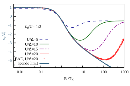
Figure 4: Evolution of $c_{V}$ during the crossover to the Kondo limit. The normalized FL transport coefficient $c_{V}/c_{V}^{K}$ is plotted as a function of $B/T_{K}$ for several values of $U/\Delta$, including the Kondo limit (thick solid line). The direct integration of the coupled Bethe Ansatz equations, Eq. (S3a) and (S4b) Note (1), performed here for $U/\Delta=20$ (BAE, open dots), is in very good agreement with the corresponding Wiener-Hopf solution (dashed line). All curves with large $U/\Delta$ ($\gtrsim 10$) initially collapse onto a universal scaling curve as function of increasing $B/T_{K}$, but for large $B/T_{K}$ they eventually bend upward towards zero at a field scale that increases with $U/\Delta$ and tends to infinity in the Kondo limit.

Away from particle-hole symmetry, where the Wiener-Hopf method is not applicable, the Bethe Ansatz coupled integral equations (see Eq. (S3a) and (S3b) in the Supplemental Material Note (1)) have to be solved numerically. This direct method is used in Figs. 6 and 7. In Fig. 4 we have verified that at particle-hole symmetry it agrees nicely with the accurate Wiener-Hopf solution.

To conclude this subsection, we briefly discuss some special cases, for future reference:

(i) Zero magnetic field: Eqs. (13) for the odd FL parameters yield zero for $B=0$,

$$\overline{\alpha}_{1}=\overline{\alpha}_{2}=\overline{\phi}_{2}=0\,,$$ (15)

since $m_{d}$ is an antisymmetric function of $B$.

(ii) Particle-hole symmetry: At ${\varepsilon_{d}}=-U/2$ we have

$$n_{d}=1,\;\;\delta_{0\sigma}=\pi\left(\tfrac{1}{2}+\sigma m_{d}\right),\;\;\overline{\alpha}_{1}=\alpha_{2}=\phi_{2}=0,$$ (16)

for any $B$. The three FL parameters vanish since $n_{d}-1$ is an antisymmetric function of ${\varepsilon_{d}}-U/2$, implying the same for $\chi_{m}$ and $\partial\chi_{c}/\partial{\varepsilon_{d}}$, so that both vanish at ${\varepsilon_{d}}=-U/2$.

(iii) Kondo limit: If the limit $U/\Delta\to\infty$ is taken at particle-hole symmetry while maintaining a finite Kondo temperature, local charge fluctuations are frozen out completely and the Anderson model maps onto the Kondo model. All susceptibilities involving derivatives of $n_{d}$ with respect to ${\varepsilon_{d}}$ vanish, namely $\chi_{c}=\chi_{m}=\partial_{{\varepsilon_{d}}}\chi_{c}=\partial_{{\varepsilon_{d}}}\chi_{s}=\partial_{B}\chi_{c}=0$, so that Eqs. (16) are supplemented by

$$\frac{\alpha_{1}}{\pi}=\frac{\phi_{1}}{\pi}=\chi_{s},\qquad\frac{4\overline{\alpha}_{2}}{\pi}=\frac{\overline{\phi}_{2}}{\pi}=2\frac{\partial\chi_{s}}{\partial B}\,.$$ (17)

Since $\chi_{s}$ and $\partial\chi_{s}/\partial B$ are strictly positive and negative, respectively, the same is true for $\alpha_{1},\phi_{1}$ and $\overline{\alpha}_{2},\overline{\phi}_{2}$.

(iv) Kondo limit at large fields: In the limit $B\gg T_{K}$ of the Kondo model, its Bethe Ansatz solution yields the following results for the leading asymptotic behavior of the magnetization and its derivates, with $\beta_{r}=\frac{\pi}{8}(B/T_{K})^{2}$:

$$m_{d} =\frac{1}{2}-\frac{1}{2\ln\beta_{r}},\quad\chi_{s}=\frac{1}{B\,(\ln\beta_{r})^{2}},$$ (18a)

$$\frac{\partial\chi_{s}}{\partial B} =-\frac{1}{B^{2}\,(\ln\beta_{r})^{2}}.$$ (18b)

Thus, all the FL parameters in Eq. (17) vanish asymptotically in the large-field limit.

II.5 Characteristic FL energy scale

As mentioned repeatedly above, the FL approach only holds for excitation energies sufficiently small, say $|\varepsilon-{\mu_{0\sigma}}|\ll E_{\ast}$, that all terms in expansion (7) for $\delta_{\sigma}(\varepsilon,n_{\sigma^{\prime}})-{\delta_{0\sigma}}$ are small. In the local moment regime of the Anderson model, the FL scale $E_{\ast}$ can be associated with the Kondo temperature $T_{K}$, but in the present context we need a definition applicable in the full parameter space of the Anderson model. Following Ref. Mora et al., 2015, we define $E_{\ast}$ in terms of the FL coefficient of the leading term in expansion (7),

$$E_{\ast}=\frac{\pi}{4\alpha_{1}}=\frac{1}{4\chi_{s}+\chi_{c}}\,,$$ (19)

and $T_{K}$ in terms of the zero-field spin susceptibility,

$$T_{K}=\frac{1}{4\chi_{s}^{B=0}}\,.$$ (20)

While both definitions involve some arbitrariness, they are mutually consistent, in that the zero-field value of $E_{\ast}$ equals $T_{K}$ in the Kondo limit $U/\Delta\to\infty$, where we have

$$E_{\ast}^{B=0}=T_{K},\qquad E_{\ast}^{B\gg T_{K}}=\tfrac{1}{4}B(\ln\beta_{r})^{2}\,.$$ (21)

More generally, $E_{\ast}^{B=0}$ and $T_{K}$ are roughly equal throughout the local-moment regime where $\chi_{c}\simeq 0$, i.e. for $U\gg\Delta$ and $-U+\Delta\lesssim{\varepsilon_{d}}\lesssim-\Delta$. In this regime, $T_{K}$ is well described by the analytic formula (af) Haldane (1978a, b); Mora et al. (2015)

$$T_{K}^{\rm(af)}=\sqrt{\tfrac{U\Delta}{2}}\,e^{\pi\left[\frac{\Delta}{2U}-\frac{U}{8\Delta}\right]}e^{x^{2}}\,,\quad$$ (22)

where $x=({\varepsilon_{d}}+U/2)\sqrt{\pi/(2\Delta U)}$ measures the distance to the particle-hole symmetric point. At the latter, $T_{K}^{\rm(af)}|_{x=0}$ can be derived analytically from the Bethe-Ansatz equations for $\chi_{s}^{B=0}$ Tsvelick and Wiegmann (1983a). The factor $e^{x^{2}}$, familiar from Haldane’s RG treatment of the Anderson model Haldane (1978a), phenomenologically includes the effect of particle-hole asymmetry. Throughout the local moment regime, Eq. (22) yields excellent agreement with a direct numerical evaluation of Eq. (20) via the Bethe-Ansatz equations for $\chi^{B=0}_{s}$ (see Fig. 6 below).

III Spectral function and non-linear conductance

III.1 General results

For the remainder of this paper we consider a single-level quantum dot with symmetric tunnel couplings to left and right leads with chemical potentials $\pm eV/2$, described by the two-lead, single-level Anderson model. The non-linear conductance of this system can be expressed by the Meir-Wingreen formula as Meir and Wingreen (1992)

$$G(V,T)=\partial_{V}\frac{e}{h}\int_{\varepsilon}\left[f_{L}(\varepsilon)-f_{R}(\varepsilon)\right]A(\varepsilon)\,.$$ (23)

Here $f_{L/R}(\varepsilon)=[e^{(\varepsilon\mp eV/2)/T}\!+\!1]^{-1}$ are the distribution functions of the left and right leads, $A(\varepsilon)=\sum_{\sigma}A_{\sigma}(\varepsilon)$ is the local spectral function with spin components $A_{\sigma}(\varepsilon)=-\pi\nu_{0}\,\text{Im}\mathcal{T}_{\sigma}(\varepsilon)$, and $\mathcal{T}_{\sigma}(\varepsilon)$ is the $T$-matrix for spin $\sigma$ conduction electrons scattering off the local level. A FL calculation of the low-energy behavior of $A_{\sigma}(\varepsilon)$ and $G(V,T)$ has been performed in detail at zero magnetic field in Ref. Mora et al., 2015, following similar studies in Refs. Mora et al., 2008; Vitushinsky et al., 2008; Mora et al., 2009; Hörig et al., 2014. The strategy of the calculation is rather straightforward. First one introduces even and odd linear combinations of operators from the two leads. The odd ones decouple, resulting in an effective one-lead Anderson model for a dot coupled to the even lead, whose low-energy behavior is described by the Hamiltonian $H_{\rm FL}$ introduced above. Then, in the spirit of the standard Landauer-Büttiker formalism Blanter and Büttiker (2000), the current operator is expanded over a convenient single-particle basis of scattering states accounting for both the lead-dot geometry and the FL elastic phase shifts. Interactions between electrons stemming from $H_{\phi}$ are included perturbatively when calculating the average current in the Keldysh formalism Kamenev and Levchenko (2009).

The calculation described above trivially generalizes to the case of nonzero field, since the two spin components give separate contributions to the current. The results from Ref. Mora et al., 2015 for the low-energy expansion of the conductance can thus be directly taken over, modified merely by supplying FL parameters with spin indices. A corresponding low-energy expansion for the spectral function can then be deduced via Eq. (23). We now present the results obtained in this manner, starting with the $T$-matrix and spectral function, since these form the basis for understanding the resulting physical behavior.

For the $T$-matrix, written as the sum of elastic and inelastic contributions, the results of Ref. Mora et al. (2015) (Supplementary Section S-V) imply

$${\cal T}^{\rm el}_{\sigma}(\varepsilon) =-\frac{i}{2\pi\nu_{0}}\left(1-e^{2i\delta_{\sigma}(\varepsilon)}\right),$$ (24a)

$${\cal T}^{\rm inel}_{\sigma}(\varepsilon) =-\frac{ie^{2i{\delta_{0\sigma}}}}{2\pi\nu_{0}}\phi_{1}^{2}\left[\varepsilon^{2}+(\pi T)^{2}+\tfrac{3}{4}(eV)^{2}\right].$$ (24b)

Here ${\cal T}^{\rm el}_{\sigma}(\varepsilon)$ is determined by the phase shift $\delta_{\sigma}(\varepsilon)$ obtained from Eq. (7) using $n_{\sigma}(\varepsilon)=\frac{1}{2}\left[f_{L}(\varepsilon)+f_{R}(\varepsilon)\right]$ as quasiparticle distribution function for the even lead:

$$\delta_{\sigma}(\varepsilon)={\delta_{0\sigma}}\!+\!\alpha_{1\sigma}\varepsilon\!+\!\alpha_{2\sigma}\varepsilon^{2}\!-\!\tfrac{1}{12}\phi_{2\bar{\sigma}}\!\left[(\pi T)^{2}\!+\!\tfrac{3}{4}(eV)^{2}\right]\!.$$ (25)

(In Ref. Filippone et al. (2017) this equation contained an error, which lead to incorrect physical conclusions, see Ref. .) Note that the inelastic $T$-matrix has the same dependence on temperature and bias, which occur only in the combination $(\pi T)^{2}\!+\!\frac{3}{4}(eV)^{2}$ . This is significant, since it implies that knowing the spectral function’s leading temperature dependence in equilibrium suffices to deduce its leading bias dependence in nonequilibrium. The spectral function, expanded to second order in $\varepsilon$, $T$ and $eV$, can thus be written as

$$A(\varepsilon)=A_{0}+A_{1}\varepsilon-\widetilde{C}_{\!A}\!\left[\tfrac{1}{3}(\pi T)^{2}\!+\!\tfrac{1}{4}(eV)^{2}\right]-C_{\!A}\varepsilon^{2},$$ (26)

with expansion coefficients:

$$A_{0} =\sum_{\sigma}\sin^{2}({\delta_{0\sigma}}),\quad A_{1}=\sum_{\sigma}\alpha_{1\sigma}\sin(2{\delta_{0\sigma}}),$$ (27a)

$$\widetilde{C}_{\!A} =-\sum_{\sigma}\left[\tfrac{3}{2}\phi_{1}^{2}\cos(2{\delta_{0\sigma}})-\tfrac{1}{4}\phi_{2\bar{\sigma}}\sin(2{\delta_{0\sigma}})\right]\!,$$ (27b)

$$C_{\!A} =-\sum_{\sigma}\!\left[(\alpha_{1\sigma}^{2}\!+\!\tfrac{1}{2}\phi_{1}^{2})\cos(2{\delta_{0\sigma}})+\alpha_{2\sigma}\sin(2{\delta_{0\sigma}})\right]\!.$$ (27c)

These results hold for all values of $U$, $\Delta$, $\varepsilon_{d}$ and $B$.

Inserting Eq. (26) into (23) and using the relations

$$\partial_{V}\!\!\int_{\varepsilon}\left[f_{L}\!-\!f_{R}\right]\varepsilon^{2}=e\left[\tfrac{1}{3}(\pi T)^{2}\!+\!\tfrac{1}{4}(eV)^{2}\right],$$ (28)

$$\partial_{V}\!\!\int_{\varepsilon}\left[f_{L}\!-\!f_{R}\right]\!\left[\tfrac{1}{3}(\pi T)^{2}\!+\!\tfrac{1}{4}(eV)^{2}\right]=e\!\left[\tfrac{1}{3}(\pi T)^{2}\!+\!\tfrac{3}{4}(eV)^{2}\right]\!,$$

one obtains an expansion for the conductance of the form

$$G(V,T) =\widetilde{G}-(2e^{2}/h)\left[C_{T}T^{2}+C_{V}(eV)^{2}\right].$$ (29)

Here $\widetilde{G}=\frac{1}{2}A_{0}G_{0}$ is the zero-temperature, linear conductance, $G_{0}=2e^{2}/h$ is the conductance quantum, and the expansion coefficients of the quadratic terms are

$$C_{T} =\tfrac{1}{6}\pi^{2}(\widetilde{C}_{\!A}+C_{\!A})\,,\quad C_{V}=\tfrac{3}{8}(\widetilde{C}_{\!A}+\tfrac{1}{3}C_{\!A})\,.$$ (30)

Eqs. (30) and (27) are consistent with expressions for $C_{T}$ and $C_{V}$ recently derived by Oguri and Hewson Oguri and Hewson (2018a); *Oguri2017a; *Oguri2017b (see Appendix C).

The four $C$ coefficients introduced above all have dimensions of (energy)^-2. If we express them as

$$\widetilde{C}_{\!A}=\frac{\tilde{c}_{A}}{E_{\ast}^{2}},\quad C_{X}=\frac{c_{X}}{E_{\ast}^{2}},\quad X=A,V,T\,,$$ (31)

where $E_{\ast}$ is the FL scale of Eq. (19), the resulting four $c$ coefficients are dimensionless, with $c_{T}$ and $c_{V}$ corresponding to the coefficients calculated in Ref. Mora et al., 2015. For asymmetric couplings to the leads Aligia (2012); Muñoz et al. (2013); Aligia (2014), not considered here, the conductance also contains a term linear in $V$, as also discussed in Ref. Mora et al. (2009), where the same formalism has been applied.

Equations (27) instructively reveal which role the various FL parameters play in determining the shape of the local spectral function $A(\varepsilon)$ at the chemical potential, characterized by its “height” $A(0)$, slope $A_{1}$ and curvature $C_{\!A}$. The ground state phase shifts ${\delta_{0\sigma}}$ fix the height at zero temperature and bias, $A_{0}$. The elastic couplings $\alpha_{1\sigma}$ and $\alpha_{2\sigma}$ of $H_{\alpha}$ affect only the slope and curvature, but not the height. The inelastic couplings $\phi_{1}$ and $\phi_{2\sigma}$ of $H_{\phi}$ determine the leading effect of temperature and bias on the height via $\widetilde{C}_{\!A}$, while $\phi_{1}$ also contributes to the curvature $C_{\!A}$. Moreover, via the sine and cosine factors the relative contributions of all terms depend sensitively on the ground state phase shifts ${\delta_{0\sigma}}$, and hence can change significantly when these are tuned via changing parameters such as $B$ or ${\varepsilon_{d}}$.

III.2 Spectral function at particle-hole symmetry

When the single-level, two-lead Anderson model is tuned into the local moment regime, the local spectral function exhibits a Kondo peak that splits with magnetic field. Correspondingly, the non-linear conductance exhibits a zero-bias peak that likewise splits with increasing field. Our goal is to use FL theory to study the peak splittings of both the spectral function and the nonlinear conductance in quantitative detail. For this purpose, we will focus on the particle-hole symmetric point in this subsection and the next, leaving particle-hole asymmetry to Subsection III.4.

We begin with a qualitative discussion, based on the results of numerous previous studies of the local moment regime Costi (2000); Wright et al. (2011); Zitko et al. (2009); Moore and Wen (2000); Glazman and Pustilnik (2005); Rosch et al. (2003, 2005); Weichselbaum et al. (2009). At zero field, the two components of the local spectral function, $A_{\uparrow}$ and $A_{\downarrow}$, both exhibit a Kondo peak at zero energy. An increasing field weakens these peaks and shifts them in opposite directions. When their splitting exceeds their width, which happens for $B$ of order $T_{K}$, then $A=A_{\uparrow}+A_{\downarrow}$ develops a local minimum at zero energy, implying that $C_{\!A}$ changes from positive to negative. We will denote the “splitting field” where $C_{\!A}=0$ by $B_{A}$. [For $B\gg T_{K}$ the subpeaks in $A_{\uparrow,\downarrow}$ are located at $\varepsilon\simeq\pm B$, modulo corrections of order $\mp B/\log(B/T_{K})$ Moore and Wen (2000); Rosch et al. (2003); Weichselbaum et al. (2009).]

For small fields, where the Kondo peak is well developed, an increasing temperature or bias tends to weaken it, thus reducing the zero-energy spectral height $A(0)$. We thus expect $\widetilde{C}_{\!A}$ to be a decreasing but positive function of $B$ for small fields. However, this trend can be expected to be reversed for fields of order $T_{K}$ or larger, where Kondo correlations are weak or absent, in which case we may expect $\widetilde{C}_{\!A}$ to become negative. We will denote this field by $\widetilde{B}_{A}$.

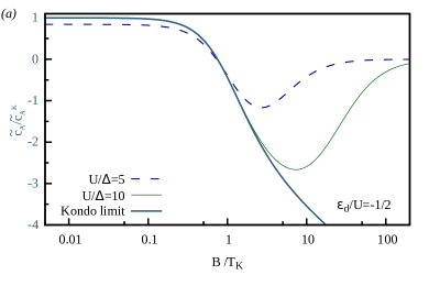
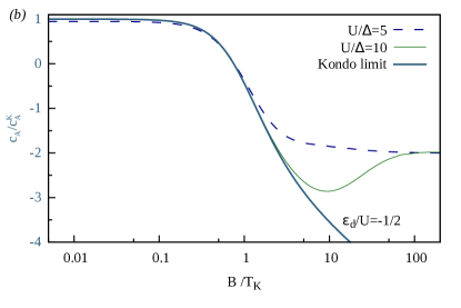
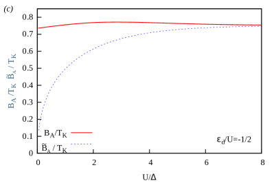
Figure 1: Low-energy properties of the spectral function at particle-hole symmetry. (a) The normalized height coefficient $\tilde{c}_{A}/\tilde{c}_{A}^{K}$ and (b) curvature coefficient $c_{A}/c_{A}^{K}$ of the local spectral function at particle-hole symmetry, plotted as functions of magnetic field [in units of $T_{K}$, as defined in Eq. (20)], for three values of the interaction parameter $U/\Delta$, including the Kondo limit $U/\Delta=\infty$ [given by Eq. (35)]. The sign change for $C_{\!A}$ signals the splitting of the Kondo resonance into two resonances due to the breaking of the Kondo singlet by the magnetic field. (c) The characteristic fields $B_{A}$ and $\widetilde{B}_{A}$ where $C_{\!A}$ and $\widetilde{C}_{\!A}$ vanish, respectively, plotted in units of $T_{K}$ as functions of $U/\Delta$. In the Kondo limit $U/\Delta\to\infty$ they approach the same limiting value, $B_{A}=\widetilde{B}_{A}=0.75073T_{K}$.

To study this behavior quantitatively, we specialize the results of the previous subsection to the case of particle-hole symmetry using Eq. (16), obtaining:

$$A_{0} =2\cos^{2}(\pi m_{d})\,,$$ (32a)

$$\widetilde{C}_{\!A} =3\phi^{2}_{1}\cos(2\pi m_{d})+\tfrac{1}{2}\overline{\phi}_{2}\sin(2\pi m_{d})\,,$$ (32b)

$$C_{\!A} =\left(2\alpha_{1}^{2}+\phi^{2}_{1}\right)\cos(2\pi m_{d})+2\overline{\alpha}_{2}\sin(2\pi m_{d})\,.$$ (32c)

Figure 1 shows the $B$-dependence of $\tilde{c}_{A}=E_{\ast}^{2}\widetilde{C}_{\!A}$ and $c_{A}=E_{\ast}^{2}C_{\!A}$ for several values of $U/\Delta$. (We multiply by the $B$-dependent scale $E_{\ast}^{2}$ [cf. Eq. (31)], since this better reveals the large-field behavior, for reasons explained below.)

The main finding of Fig. 1 is that with increasing field, both $c_{A}$ and $\tilde{c}_{A}$ decrease and change sign, as expected from our qualitative discussion. The sign change for $c_{A}$ implies that our FL approach reproduces the field-induced splitting of the Kondo peak in the spectral function. Moreover, we find [Fig. 1(c)] that the scale for the fields $B_{A}$ and $\widetilde{B}_{A}$ is universal, in the usual sense familiar from many aspects of Kondo physics in the Anderson model: the ratios $B_{A}/T_{K}$ and $\widetilde{B}_{A}/T_{K}$ are of order unity and depend only weakly on $U/\Delta$, tending to a constant value in the Kondo limit $U/\Delta\to\infty$. Their limiting value, namely $B_{A}=\widetilde{B}_{A}=0.75073\,T_{K}$, agrees with previous numerical estimates Costi (2000); Wright et al. (2011).

Another observation from Fig. 1 is that $c_{A}$ and $\tilde{c}_{A}$ show a very similar field dependence for $B/T_{K}\lesssim 1$. In the large-field regime their field dependence differs somewhat for weak interactions, $U/\Delta\lesssim 5$, but becomes increasingly similar with increasing $U/\Delta$. To understand their behavior in the Kondo limit $U/\Delta\to\infty$, we first consider that of $\widetilde{C}_{\!A}$ and $C_{\!A}$. Eqs. (32) and (17) show that they are equal in this limit, given by

$$\widetilde{C}_{\!A}=C_{\!A}=3\alpha^{2}_{1}\cos(2\pi m_{d})+2\overline{\alpha}_{2}\sin(2\pi m_{d})\,,$$ (33)

with zero-field values (indicated by a superscript $K$ for “fully-developed Kondo effect”) of

$$\widetilde{C}_{\!A}^{K} =C_{\!A}^{K}=\frac{3\pi^{2}}{16}\frac{1}{T_{K}^{2}}\quad(B=0)\,,$$ (34a)

and asymptotic large-field behavior [obtained via (18)]

$$\widetilde{C}_{\!A}=C_{\!A}=-\frac{\pi^{2}}{B^{2}(\ln\beta_{r})^{4}}\ln\beta_{r}\quad(B\gg T_{K})\,.$$ (34b)

This confirms that $\widetilde{C}_{\!A}$ and $C_{\!A}$ both become negative at large fields. Their magnitude changes in scale from $\sim 1/T_{K}^{2}$ for small fields to becoming negligibly small, $\sim 1/[B^{2}(\ln\beta_{r})^{3}]$, for large fields. We now also see why it is useful to study the $C$ coefficients in the normalized form $c=E_{\ast}^{2}C$ of Eq. (31), as done in Fig. 1: $E_{\ast}^{2}$ increases with $B$ and in the large-field limit [see (21)] compensates the small prefactor in Eq. (34b). Correspondingly normalized, Eqs. (33) and (34) yield

$$\frac{\tilde{c}_{A}}{\tilde{c}_{A}^{K}}=\frac{c_{A}}{c_{A}^{K}} =\cos(2\pi m_{d})+\frac{\partial_{B}\chi_{s}}{3\pi\chi_{s}^{2}}\sin(2\pi m_{d})\,,$$ (35)

with zero-field values and large-field behavior given by

$$\tilde{c}_{A}^{K} =c_{A}^{K}=\frac{3\pi^{2}}{16}\,, (B=0)\,,$$ (36a)

$$\frac{\tilde{c}_{A}}{\tilde{c}_{A}^{K}} =\frac{c_{A}}{c_{A}^{K}}=-\tfrac{1}{3}\ln\beta_{r} (B\gg T_{K})\,.$$ (36b)

The $-\ln\beta_{r}$ term in Eq. (36b) explains the behavior of the Kondo limit curves (thick solid) in Figs. 1(a) and 1(b).

As a consistency check, we note that inserting the Kondo-limit coefficients $\widetilde{C}_{\!A}^{K}$ and $C_{\!A}^{K}$ of Eq. (34a) into Eq. (26) for $A(\varepsilon)$ yields the low-energy expansion of the spectral function of the spin-$\frac{1}{2}$ Kondo model at $B=0$. Indeed, the result so obtained,

$$A^{K}(\varepsilon)=2-\frac{3\pi^{2}}{16}\frac{\left[\varepsilon^{2}+\frac{1}{3}(\pi T)^{2}+\frac{1}{4}(eV)^{2}\right]}{T_{K}^{2}}\,,$$ (37)

is consistent with previous studies of the Kondo model for $V=0$ Nozières (1974a); Affleck and Ludwig (1993); Glazman and Pustilnik (2005); Hanl et al. (2014) [see for example Eq. (4) of Ref. Hanl et al. (2014), where the coefficients of this expansion, called $c_{\varepsilon}$ and $c^{\prime}_{T}$ there, were checked numerically using NRG].

For completeness, we mention that the opposite limit of weak interactions yields, for ${\varepsilon_{d}}=U=0$:

$$\tilde{c}_{A}=0,\qquad c_{A}=\frac{\pi^{2}}{8}\frac{\Delta^{2}-3B^{2}/4}{\Delta^{2}+B^{2}/4}\,.$$ (38)

III.3 Conductance at particle-hole symmetry

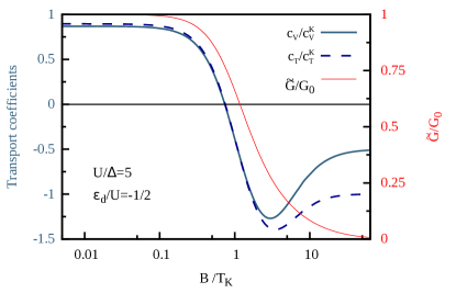
Figure 2: FL transport properties at particle-hole symmetry and $U/\Delta=5$, plotted as functions of $B/T_{K}$. Left axis: Normalized FL transport coefficients $c_{V}/c_{V}^{K}$ (thick solid line) and $c_{T}/c_{T}^{K}$ (thick dashed line). The fields $B_{T}$ and $B_{V}$ where $c_{T}$ and $c_{V}$ change sign are essentially equal and of order $T_{K}$. Right axis: Normalized zero-temperature linear conductance $\tilde{G}/G_{0}=\cos^{2}(\pi m_{d})$ [from Eq. (32a)] (thin solid line).

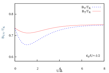
Figure 3: Interaction dependence of splitting field properties at particle-hole symmetry, plotted as functions of $U/\Delta$. Splitting fields $B_{T}$ and $B_{V}$ at which $c_{T}$ and $c_{V}$ vanish (left axis, thick line), shown in units of $T_{K}$. In the absence of interaction $U=0$, the Kondo temperature extracted from Eq. (20) is $T_{K}=\pi\Delta/2$, hence $B_{V}=B_{T}=\frac{4}{\pi\sqrt{3}}~{}T_{K}\simeq 0.735~{}T_{K}$. In the Kondo limit $U/\Delta\to\infty$, both curves approach the limiting value $B_{V}=B_{T}=0.75073~{}T_{K}$. The data also agrees with NRG to within the NRG’s error bars (see Fig. 9 in Appendix D).

We now turn our attention to transport properties, and again begin with a qualitative discussion. The behavior of the local spectral function discussed in the preceding subsection fully determines, via the Meir-Wingreen formula (23), that of the non-linear differential conductance. At zero field $G(V,T)$, studied as function of $V$, exhibits a peak around zero bias which weakens with temperature, and which splits with increasing field.

The details of these changes are quantified by Eq. (30): as $\tilde{c}_{A}$ and $c_{A}$ decrease with increasing field and eventually turn negative, the same will happen for $c_{T}$ and $c_{V}$. We will denote the “splitting fields” at which $c_{T}$ or $c_{V}$ equal zero by $B_{T}$ or $B_{V}$, respectively. Since in Eq. (30) the relative weight of $\tilde{c}_{A}$ to $c_{A}$ is three times larger in $c_{V}$ than in $c_{T}$, the behavior of these two coefficients, and that of the corresponding splitting fields $B_{V}$ and $B_{T}$, can thus differ quantitatively.

In the noninteracting limit, where $\tilde{c}_{A}=0$, $c_{T}$, $c_{V}$ and $c_{A}$ are proportional to each other for all fields, $c_{V}=\frac{3}{4\pi^{2}}c_{T}=\frac{1}{4}c_{A}$, implying splitting fields of $B_{T}=B_{V}=(2/\sqrt{3})\Delta$ [see Eq. (38)]. At this field value, the magnetization equals $\frac{1}{6}$ and the zero-temperature linear conductance is $\widetilde{G}=\frac{3}{2}e^{2}/h$, i.e. $\frac{3}{4}$ of the unitary value $G_{0}=2e^{2}/h$.

With increasing $U/\Delta$, the behavior of $c_{T}$ and $c_{V}$ are strikingly similar for small fields and begin to differ only for fields well above $T_{K}$. This is already evident in Fig. 2, which shows the $B$ dependence of $\widetilde{G}$, $c_{T}$ and $c_{V}$ for $U/\Delta=5$. With increasing field, $\widetilde{G}$ is smoothly suppressed on a field scale set by $T_{K}$, while $c_{T}$ and $c_{V}$ both decrease and change sign, at essentially the same scales: $B_{T}$ and $B_{V}$ are both of order $T_{K}$, a property that they directly inherit from $B_{A}$ and $\widetilde{B}_{A}$. However, the large-field values reached by $c_{T}$ and $c_{V}$ for $B\gg T_{K}$ are different. For $U/\Delta$ not too large $(\lesssim 5$, as in Fig. 2), they correspond to the empty-orbital asymptotic forms found in Ref. Mora et al., 2015,

$$c^{\rm eo}_{T}=-\frac{\pi^{4}}{16},\qquad c^{\rm eo}_{V}=-\frac{3\pi^{2}}{64}.$$ (39)

A systematic study of the splitting fields $B_{T}$ and $B_{V}$ as functions of $U/\Delta$ yields the results shown in Fig. 3. They show qualitatively similar behavior, remaining of order $T_{K}$ for all values of $U/\Delta$. This implies that $B_{T}$ and $B_{V}$ are universal in the same sense as $B_{A}$.

In the Kondo limit, Eqs. (30), (33) and (34) yield

$$\frac{c_{T}}{c_{T}^{K}}=\frac{c_{V}}{c_{V}^{K}}=\cos(2\pi m_{d})+\frac{\partial_{B}\chi_{s}}{3\pi\chi_{s}^{2}}\sin(2\pi m_{d}),$$ (40)

with zero-field values and large-field behavior given by

$$c_{T}^{K} =\frac{\pi^{4}}{16},\qquad c_{V}^{K}=\frac{3\pi^{2}}{32} (B=0),$$ (41a)

$$\frac{c_{T}}{c_{T}^{K}} =\frac{c_{V}}{c_{V}^{K}}=-\tfrac{1}{3}\ln\beta_{r} (B\gg T_{K}).$$ (41b)

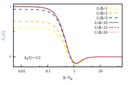
Figure 5: The coefficient $C_{V}=c_{V}/E_{\ast}^{2}$, plotted as a function of $B/T_{\rm K}$ for different interaction strengths $U/\Delta$, in units of $C_{V}^{\rm K}=c_{V}^{\rm K}/T_{K}^{2}$, with $c_{V}^{\rm K}$ defined in Eq. (41a). In contrast to $c_{V}$ from Fig. 4(a), $C_{V}$ is strongly suppressed in the regime $B>T_{K}$ (even for $U/\Delta\gg 1$), because for large fields the spin susceptibility becomes very small and hence $E_{\ast}$ very large [cf. Eq. (21)]. Inset: the normalization factor $C_{V}^{\rm K}$, plotted as function of $U/\Delta$ in units of $1/\Delta^{2}$ (black points indicate the $U/\Delta$ values from the main plot). $C_{V}^{\rm K}$ shows an exponential increase with $U/T_{K}$, caused by an exponential decrease in $T_{K}$. The growth in $C_{V}^{\rm K}$ is counteracted by the fact that the voltage window in which our FL analysis applies decreases exponentially, since the FL expansion (29) of the conductance requires $V\ll T_{K}$.

To conclude this section, we remark that it is instructive to compare the predictions of our FL theory with those of Hewson, Bauer and Oguri Hewson et al. (2005), who computed $B_{V}$ for the case of particle-hole symmetry using renormalized perturbation theory (RPT) [see the discussion after their Eqs. (19) and (27)]. For example, for $U/\Delta=4\pi$ they find $\tfrac{1}{2}B_{V}\simeq 0.584T_{K}$ [after their Eq. (27)]. This is comparable in magnitude, but not equal, to our result $B_{V}\simeq 0.7506\,T_{K}$ [see our Fig. 3] for the same value of $U/\Delta$. However, we note that in Ref. Hewson et al. (2005) the coefficients playing the roles of our $\alpha_{2\sigma}$ and $\phi_{2\sigma}$ were computed perturbatively in terms of the renormalized parameters of RPT (the same three parameters are also used at zero magnetic field Hewson (2005)), and are therefore approximate. As noted in the concluding section of Ref. Mora et al. (2015), it is not clear whether this RPT approach contains enough parameters to accurately evaluate $B_{V}$.

In an attempt to track down the difference, we have expressed our FL parameters in terms of the RPT parameters needed in general to characterize the local impurity Green’s function (see Appendix B). This can be done by simply expanding the RPT spectral function to second order in $\varepsilon$, $T$ and $eV$ and equating the result to our Eqs. (26) and (27). The resulting equations (64) provide a RPT-FL dictionary that relates the RPT parameters to our FL parameters. Since the latter are computable exactly via the Bethe Ansatz, this dictionary provides a number of exact constraints on the RPT parameters. We were not able to ascertain that the expressions provided in Ref. Hewson et al. (2005) for their RPT parameters satisfy these constraints. We suspect that at finite magnetic field or out of particle-hole symmetry, the second-order RPT (perturbative in the renormalized interaction $U$) becomes approximate for the calculation of the coefficients $\alpha_{2}$ and $\phi_{2}$ Hewson (2016). However, we would like to suggest a converse strategy: one could set up a RPT whose input parameters are computed exactly by Bethe Ansatz via the RPT-FL dictionary in Appendix B. Doing so would be an interesting goal for future work, since RPT offers the welcome prospect of smoothly linking the exact FL description of the impurity’s low-energy behavior to a description, albeit approximate, that is also useful at higher energies.

Very recently, Oguri and Hewson have taken a decisive step forward which completes the RPT program and puts it on a fully rigorous footing Oguri and Hewson (2018a); *Oguri2017a; *Oguri2017b: they used Ward identities together with the analytic and antisymmetry properties of the vertex function of the Anderson impurity model to fully determine all parameters needed in RPT. In doing so, they also presented a microscopic derivation of the FL relations arising from a low-energy expansion of the self-energy and the vertex. Their results are in full agreement with the FL theory presented in section II of this work. Indeed, we show in appendix C that our analytical expressions for $C_{T}$ and $C_{V}$ coincide, for general values of $\varepsilon_{d}$, with those obtained by them. For the case of particle-hole symmetry, they combined their FL analysis with NRG computations of the FL parameters. Their prediction for the splitting field for the zero-bias conductance peak is $B_{V}/2=h_{V}\simeq 0.4T_{K}$ for $U/\Delta=4\pi$, implying $B_{V}/T_{K}\simeq 0.8$. This is in fairly good agreement with our prediction at $U/\Delta=4\pi$, namely $B_{V}/T_{K}=0.7506$. The difference is likely due to different methods for numerically determining the FL parameters – NRG in their work, Bethe Ansatz in ours.

As another consistency check for our FL analysis, we have used NRG to compute the equilibrium spectral function $A(\epsilon)$ and extracted $C_{T}$ and $C_{V}$ from its leading dependence on $T$ and $\epsilon$. The results of this analysis, presented in Appendix D, are consistent with the FL results for $C_{T}$ and $C_{V}$ of Fig. 2, and $B_{T}$ and $B_{V}$ of Fig. 3.

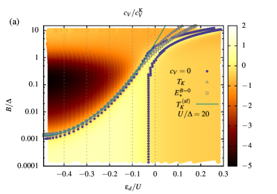
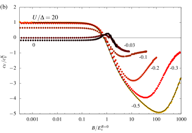
Figure 6: (a) Transition from the local-moment regime to the empty-orbital regime for the transport coefficient $c_{V}/c_{V}^{K}$, shown using a color scale, as a function of the magnetic field $B$ and the level energy $\varepsilon_{d}$, at $U/\Delta=20$, a convenient value to highlight features related to Kondo physics. The solid line shows the prediction for the Kondo scale of the analytic formula (22) for $T_{K}^{\rm(af)}$, the grey triangles the numerical evaluation of $T_{K}$ as defined in Eq. (20) and the grey squares the numerical evaluation of $E_{*}$ in Eq. (19) for $B=0$. All these quantities show a nice agreement as long as $\varepsilon_{d}<0$. The blue points signal when $c_{V}=0$ and changes sign. The light-colored regions correspond to positive values of $c_{V}$. (b) Same quantity $c_{V}/c_{V}^{K}$ as in (a), now shown along the cuts marked in (a) by grey dashed lines, and plotted as a function of $B/E_{*}^{B=0}$ on a logarithmic scale. The numbers above the data points give the corresponding values of $\varepsilon_{d}/U$ (increasing as colors turn from light to dark). The solid line corresponds to the analytical result for $c_{V}$ at particle-hole symmetry derived from the Wiener-Hopf solution Note (1) (see also Fig. 4a). Throughout the local-moment regime in which Kondo correlations occur ($\varepsilon_{d}\lesssim-\Delta$), $c_{V}$ changes sign around fields of order $T_{K}$. For $\varepsilon_{d}\gtrsim 0$, $c_{V}$ develops a double sign change with a peak in between, which reflects a field-induced resonance between the empty- and singly-occupied dot states (see Fig. 7).

III.4 $c_{V}$ away from particle-hole symmetry

Finally, let us examine the behavior of the transport coefficient $c_{V}$ away from particle-hole symmetry. We consider only $\varepsilon_{d}/U>-\frac{1}{2}$ (from which the opposite case follows by particle-hole symmetry). The quantum dot is in a strongly correlated Kondo singlet state as long as the dot is in the local-moment regime ($-U/2\leq\varepsilon_{d}\lesssim-\Delta$). As $\varepsilon_{d}$ crosses over through the mixed-valence regime ($|{\varepsilon_{d}}|<\Delta$) into the empty-orbital regime (${\varepsilon_{d}}\gtrsim\Delta$), Kondo correlations die out completely. In the previous section, we showed that $c_{V}$ changes sign at particle-hole symmetry for splitting fields $B_{V}$ of the order of $T_{K}$ [see Fig. 3(b)]. Our aim here is to study the evolution of $B_{V}$ as $\varepsilon_{d}/U$ is tuned through the transition from the local-moment regime to the empty-orbital regime. The numerical results reported below were obtained by numerically solving the Bethe-Ansatz equations for the Anderson model Wiegmann (1980); *kawakami1982ground; *wiegmann1983; *tsvelick1983; *tsvelick1983a in the form reported in the Supplemental Material Note (1).

Fig. 6(a) shows a color-scale plot of $c_{V}$ for a large, fixed interaction of $U/\Delta=20$, plotted as function of field $B$ and level energy $\varepsilon_{d}$. Fig. 6(b) shows the same data as function of $B$ along several fixed values of ${\varepsilon_{d}}$. We find that throughout the local-moment regime, an increasing field yields a sign change for $c_{V}$ as function of $B$ around field values that distinctly follow the ${\varepsilon_{d}}$ dependence of the Kondo temperature $T_{K}$ of Eq. (20) (grey triangles). The latter is well approximated by the analytic formula $T_{K}^{\rm(af)}$ of Eq. (22) (black solid line) and coincides with the FL scale $E_{*}$ of Eq. (19) at $B=0$ (grey squares), with deviations only in the empty orbital regime (${\varepsilon_{d}}\gtrsim\Delta$).

The behavior of $c_{V}$ is strongly modified as soon as the renormalized level increases past the Fermi surface ($\varepsilon_{d}\gtrsim\Delta$) and the charge on the dot changes from 1 to 0, so that Kondo correlations are completely absent. For low magnetic fields, $c_{V}$ is negative and with increasing field evolves through a double sign change with a positive-valued peak in between, see Figs. 6 and 7. This behavior can be understood as follows. At zero magnetic magnetic field, the dot is empty and in a cotunneling regime Grabert and Devoret (2013), so that its conductance increases when the bias increases from zero. This explains why $c_{V}$ is found to be negative for small fields in Fig. 6. With increasing field, the local level is Zeeman split. When the empty and singly-occupied states come into resonance, the conductance develops a well-pronounced zero-bias peak with a negative curvature, explaining why $c_{V}$ goes through a positive-valued maximum. The resonance condition at which this happens is that the spin-up Zeeman energy $B/2$ matches the renormalized level position ${\tilde{\varepsilon}_{d}}$, which differs from ${\varepsilon_{d}}$ due to virtual processes involving doubly-occupied intermediate dot states. A perturbative calculation following Haldane Haldane (1978a) yields

$$\tilde{\varepsilon}_{d}=\varepsilon_{d}+\frac{\Delta}{\pi}\ln\frac{\varepsilon_{d}+U}{\alpha\varepsilon_{d}}\,,$$ (42)

where $\alpha$ is a constant of order one. For the choice $\alpha\simeq 1.62$ the resonance field values $B=2\tilde{\varepsilon}_{d}$, indicated by vertical solid lines in Fig. 7, indeed match the observed peak positions for $c_{V}$ rather well.

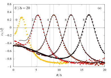
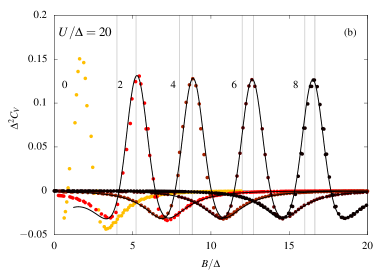
Figure 7: Magnetic-field dependence of (a) $c_{V}$ in units of $c_{V}^{\rm K}$ and (b) $C_{V}=c_{V}/E_{\ast}^{2}$ in units of $1/\Delta$, in the mixed-valence and empty-orbital regimes. Both are plotted as functions of $B/\Delta$ on a linear scale, for several values of $\varepsilon_{d}/\Delta$ (given by numbers above the data points, increasing as colors turn from light to dark). Black solid curves display analytical predictions derived in perturbation theory, showing good agreement with the numerical results (symbols). The peaks in $c_{V}$ and $C_{V}$ reflect the field-induced resonance between the empty and singly-occupied dot states. Vertical solid lines indicate the predicted values of the resonance field, $B=2\tilde{\varepsilon}_{d}$, where the renormalized level position ${\tilde{\varepsilon}_{d}}$ is given by Eq. (42) (and $\alpha\simeq 1.62$ therein); for comparison, vertical dashed lines indicate the bare values, $B=2\varepsilon_{d}$. Note that the non-trivial $B$-dependence exhibited by $C_{V}$ in (b) is as pronounced as that of $c_{V}$ in (a). The reason is that near the resonance field $B\simeq 2\tilde{\varepsilon}_{d}$, both the spin and charge susceptibilities are large, ensuring that $E_{\ast}$ remains small.

For $\varepsilon_{d}>\Delta$, the full dependence of $c_{V}$ on the magnetic field can be well captured analytically by second-order perturbation theory in the dot-lead hybridization Filippone et al. (2013), using the spin-down state of the dot as virtual intermediate state. Appendix E presents corresponding results for $n_{d\sigma}$ as function of the bare level position ${\varepsilon_{d}}$ and Zeeman field $B$, from which $c_{V}$ can be obtained using the formulas of Sec. II. Using the substitution $\varepsilon_{d}\rightarrow\tilde{\varepsilon}_{d}$ in the final results, one obtains the solid curves for $c_{V}$ shown in Fig. 7, which agree nicely with our numerical results (symbols). In the limit $\varepsilon_{d}\gg\Delta$, where the spin-down state can be totally neglected, the shape of the $c_{V}$ peak can be computed by considering a single non-interacting resonant level. The result is

$$\frac{c_{V}}{c_{V}^{\rm K}} =\frac{1}{3}\frac{\Delta^{2}-3\left(\tfrac{1}{2}B-{\varepsilon_{d}}\right)^{2}}{\Delta^{2}+\left(\tfrac{1}{2}B-{\varepsilon_{d}}\right)^{2}}\,,$$ (43)

which is peaked symmetrically around the resonance field $B=2{\varepsilon_{d}}$.

In the mixed-valence and empty-orbital regimes, the non-trivial $B$-dependence exhibited by $c_{V}$ is equally well visible in $C_{V}=c_{V}/E^{*2}$, see Fig. 7(b) (in contrast to the Kondo regime, where $C_{V}$ rapidly approaches zero for $B\gtrsim T_{K}$, cf. Fig. 5). The reason is that in the mixed-valence and empty-orbital regimes the FL scale $E_{*}$ does not become very large with increasing $B$, because both the spin and charge susceptibilities $\chi_{s}$ and $\chi_{c}$ are sizable, ensuring that $E_{\ast}$ remains small [cf. Eq. (19)]. In fact, both susceptibilities become maximal, and $E_{\ast}$ minimal, in the regime near near $B\simeq 2\tilde{\varepsilon}_{d}$ where the empty and singly-occupied dot states are in resonance. This can be checked analytically in the $\varepsilon_{d}\gg\Delta$ limit, where the perturbative approach presented in Appendix E yields

$$E_{*}=\frac{\pi}{2\Delta}\Big{[}(\varepsilon_{d}-B/2)^{2}+\Delta^{2}\Big{]}\,,$$ (44)

which is minimal at the bare resonance field $B=2{\varepsilon_{d}}$.

The fact that $C_{V}$ is large in the mixed-valence and empty-orbital regimes suggests that these regimes would be particularly suitable for the purposes of benchmarking numerical methods for solving the nonequilibrium Anderson model against the exact results obtained by our FL approach.

IV Summary and conclusions

We extended the FL framework of Ref. Mora et al., 2015 to the single-impurity Anderson model at finite magnetic field where low energy properties can be calculated in the whole phase diagram. Using a generalization of the “floating Kondo resonance” argument of Nozières, we expressed all parameters of the low-energy effective FL Hamiltonian in terms of the zero-temperature local occupation functions $n_{d\sigma}$ and their derivatives with respect to level energy and magnetic field. Our results are in full agreement with a recent analysis of Oguri and Hewson Oguri and Hewson (2018a); *Oguri2017a; *Oguri2017b. We evaluated our expressions for the FL parameters using precise Bethe Ansatz calculations. Focussing on strong interaction, zero temperature and particle-hole symmetry where the Kondo singlet forms, we obtained exact results for the magnetic-field dependence of $\tilde{c}_{A}$ and $c_{A}$, two parameters that characterize the zero-energy height and curvature of the equilibrium spectral function, respectively. We also computed the splitting field $B_{A}$ at which $c_{A}$ changes sign, signaling the onset of a field-induced splitting of the equilibrium Kondo peak, and find that $B_{A}$ is of order $T_{K}$ throughout the local-moment regime, as expected.

We next performed exact calculations of the FL transport coefficients $c_{T}$ and $c_{V}$ at particle-hole symmetry but for arbitrary magnetic fields. In the local-moment regime we find that both $c_{T}$ and $c_{V}$ change sign at a field of order $T_{K}$, as expected. Finally, we also calculated the magnetic-field dependence of $c_{V}$ throughout the crossover from the local-moment through the mixed-valence into the empty-orbital regime. Throughout the former, the behavior of $c_{V}$ is qualitatively similar to that found at particle-hole symmetry. However, it changes dramatically upon entering the empty orbital regime: there $c_{V}$ is negative at zero magnetic field, but with increasing field traverses a positive-valued peak at twice the renormalized level energy, $B\simeq 2{\tilde{\varepsilon}_{d}}$, arising from a spin-polarized resonance between the empty and singly-occupied dot states.

It would be an interesting challenge for experimental studies of nonequilibrium transport through quantum dots to check our peak-splitting predictions by detailed measurements of the nonlinear conductance as function of bias voltage and field. Since the specifics of our peak-splitting predictions are model dependent, it would be important to strive for a faithful implementation of the single-level Anderson model, requiring a small dot with a very large level spacing, and to make the ratio $U/\Delta$ as large as possible.

To conclude, we have used exact tools to address the question posed in the title of our paper, finding $B_{T}=B_{V}=0.75073T_{K}$ in the Kondo limit. On a quantitative level, our work establishes exact benchmark results against which any future numerical work on the nonequilibrium properties of the Anderson model can be tested.

Appendix A Kondo model at large magnetic field

In this appendix, we perform a consistency check of the FL theory of the main text by considering the Kondo model in the large-field limit $B\gg T_{K}$. To this end, we derive an effective FL Hamiltonian from the Kondo Hamiltonian by doing second-order perturbation theory in spin-flip scattering. This yields explicit expressions, in terms of the bare parameters of the Kondo model, for the FL parameters $\delta_{0\sigma}$, $\alpha_{j\sigma}$ and $\phi_{j\sigma}$, and hence, via the FL relations (13), also for $m_{d}$, $\chi_{s}$ and $\partial\chi_{s}/\partial B$. Satisfyingly, the latter expressions turn out to fully agree with corresponding Bethe-Ansatz results in the large-field limit.

A standard mapping exists between the Anderson model Eq. (1) and the Kondo model $H_{K}=-B\,S_{z}+\sum_{\sigma,k}\varepsilon_{k}c^{\dagger}_{k\sigma}c_{k\sigma}+H_{\rm ex}$ with the spin-exchange interaction

$$H_{\rm ex}=J\,{\bf S}\cdot{\bf s},$$ (45)

where $\mathbf{s}=\sum_{kk^{\prime}\sigma\sigma^{\prime}}c^{\dagger}_{k\sigma}\frac{{\bm{\tau}}_{\sigma\sigma^{\prime}}}{2}c_{k^{\prime}\sigma^{\prime}}$ denotes the local spin of conduction electrons and ${\bm{\tau}}_{\sigma\sigma^{\prime}}$ is a vector composed of the Pauli matrices. The mapping holds at particle-hole symmetry, where $\nu_{0}J=8\Delta/(\pi U)$, and for energies well below the charging energy $U$. The impurity then hosts exactly one electron with spin $\mathbf{S}$.

The FL Hamiltonian of Eq. (3) can be derived perturbatively at large magnetic fields $B\gg T_{K}$. A strong magnetic field polarizes the impurity and a perturbation expansion with respect to the impurity in the spin up state $|\!\uparrow\rangle$ can be formulated. The result is a perturbative Hamiltonian $H_{\rm pert}=H_{1}+H_{2}+\ldots$ written as a series with increasing powers of $J$, and in which the impurity spin has disappeared. The leading order $H_{1}$ is simply obtained by averaging the exchange Kondo term over the spin up state,

$$H_{1}=\langle\uparrow\!|H_{\rm ex}|\!\uparrow\rangle=\frac{J}{4}\sum_{\sigma,k,k^{\prime}}\sigma c^{\dagger}_{k\sigma}c_{k^{\prime}\sigma},$$ (46)

corresponding to a spin-selective potential scattering term inducing the phase shifts $\delta_{0\uparrow}=\pi-\pi\nu_{0}J/4$ and $\delta_{0\downarrow}=\pi\nu_{0}J/4$. The next order, $H_{2}$, arises from virtual impurity spin-flip process in which an electron-hole pair (with opposite spins) is excited. It is obtained by using the standard Schrieffer-Wolff technique, with the outcome

$$H_{2}=-\frac{J^{2}}{8}\sum_{\{k_{i}\}}\frac{1}{B+\varepsilon_{3}-\varepsilon_{4}}c^{\dagger}_{k_{1}\downarrow}c_{k_{2}\uparrow}c^{\dagger}_{k_{3}\uparrow}c_{k_{4}\downarrow}+\text{h.c.}$$ (47)

In order to compare this result with the FL form of Eq. (3), we normal order the two equal-spin pairs of operators in Eq. (47) with respect to a reference ground state with spin-dependent chemical potentials ${\varepsilon_{0\sigma}}=-\frac{1}{2}\sigma B_{0}$ close to ${\mu_{0\sigma}}=0$ (in the Kondo limit, where ${\varepsilon_{d}}=-\infty$, there is no need to use ${\varepsilon_{0}}\neq 0$):

$$c_{k_{2}\uparrow}c^{\dagger}_{k_{3}\uparrow} =-:\!c^{\dagger}_{k_{3}\uparrow}c_{k_{2}\uparrow}\!:+\delta_{k_{3},k_{2}}\theta(\varepsilon_{2}-\varepsilon_{0\uparrow}),$$ (48a)

$$c^{\dagger}_{k_{1}\downarrow}c_{k_{4}\downarrow} =:\!c^{\dagger}_{k_{1}\downarrow}c_{k_{4}\downarrow}\!:+\delta_{k_{1},k_{4}}\theta(\varepsilon_{0\downarrow}-\varepsilon_{1}).$$ (48b)

Inserting these expressions into Eq. (47) yields, up to a constant term, $H_{2}=H_{\alpha}+H_{\phi}$, with

$$H_{\alpha}= \frac{J^{2}\nu_{0}}{8}\!\!\!\sum_{\sigma,k_{1},k_{2}}\!\!\sigma\ln\!\left[\frac{D}{B-B_{0}+\sigma(\varepsilon_{1}\!-\!\varepsilon_{0\sigma})}\right]c^{\dagger}_{k_{1}\sigma}c_{k_{2}\sigma}$$

$$\hskip 147.95424pt+\text{h.c.}\vspace{-5mm},$$ (49)

$$H_{\phi}= \frac{J^{2}}{8}\!\sum_{\{k_{i}\}}\frac{:\!c^{\dagger}_{k_{3}\uparrow}c_{k_{2}\uparrow}c^{\dagger}_{k_{1}\downarrow}c_{k_{4}\downarrow}\!:}{B-B_{0}+(\varepsilon_{3}-{\varepsilon_{0}}_{\uparrow})-(\varepsilon_{4}-{\varepsilon_{0}}_{\downarrow})}+\text{h.c.},$$ (50)

where $D$ is the high-energy cutoff of the Kondo model. $H_{\alpha}$ describes elastic potential scattering. It can be expanded by assuming $(\varepsilon_{1,2}-{\varepsilon_{0\sigma}})\ll B-B_{0}$. The zeroth order gives the first logarithmic correction to the zero-energy phase shifts,

$$\begin{Bmatrix}\delta_{0\uparrow}\\ \delta_{0\downarrow}\end{Bmatrix}=\begin{Bmatrix}\pi\\ 0\end{Bmatrix}\mp\frac{\pi\nu_{0}J}{4}\mp\frac{\pi(\nu_{0}J)^{2}}{4}\ln\left[\frac{D}{B-B_{0}}\right].$$ (51)

Changing from wavevector to energy summations, the first and second orders obtained from Eq. (49) reproduce precisely  $H_{\alpha}$ in Eq. (3), with $\bar{\alpha}_{1}=0$, $\alpha_{2}=0$ and

$$\frac{\alpha_{1}}{\pi}=\frac{(\nu_{0}J)^{2}}{4(B-B_{0})},\qquad\frac{\overline{\alpha}_{2}}{\pi}=-\frac{(\nu_{0}J)^{2}}{8(B-B_{0})^{2}}.$$ (52)

Next, expand $H_{\phi}$ to first order in $(\varepsilon_{3,4}-{\varepsilon_{0\sigma}})/(B-B_{0})$. The result coincides with $H_{\phi}$ in Eq. (3), with $\phi_{2}=0$,

$$\frac{\phi_{1}}{\pi}=\frac{(\nu_{0}J)^{2}}{4(B-B_{0})},\qquad\frac{\overline{\phi}_{2}}{\pi}=-\frac{(\nu_{0}J)^{2}}{2(B-B_{0})^{2}}.$$ (53)

Eqs. (51) to (53) are the main results of this appendix. They explicitly give all the FL parameters in terms of the bare parameters of the Kondo model and the dummy reference energies ${\varepsilon_{0\sigma}}=-\frac{1}{2}\sigma B_{0}$, illustrating explicitly that the latter occur only in the combination $B-B_{0}$ [cf. Eq. (5)]. It is easy to verify explicitly that Eqs. (51) to (53) satisfy the FL relations (9) (in the latter, all derivatives w.r.t. ${\varepsilon_{d}}$ vanish in the Kondo limit). Moreover, the above derivation clarifies the underlying reason for why the FL parameters necessarily must be mutually interrelated: they arise as expansion coefficients of the actual physical Hamiltonian in the large-field Kondo limit, namely $H_{2}$ of Eq. (47), whose functional form fully fixes all terms in the expansion $H_{2}=H_{\alpha}+H_{\phi}+\dots$.

Eqs. (51) to (53) can also be used to test our predictions (17) for how the FL parameters are related to susceptibilities. To this end, we remove the dependence on the dummy reference energy by setting it to ${\varepsilon_{0\sigma}}={\mu_{0\sigma}}=0$ [as done in Eq. (11)]. Then, we directly compute the magnetization and spin susceptibility at large magnetic field. The Bethe Ansatz solution provides a universal expression for the magnetization of the Kondo model,

$$m_{d}=\frac{1}{2}-\frac{1}{2\pi^{3/2}}\int_{0}^{\infty}dt\,\frac{\sin(\pi t)(\beta_{r}t)^{-t}}{t}\,\Gamma\left(\tfrac{1}{2}+t\right)$$ (54)

where the ratio $\beta_{r}=\frac{\pi}{8}(B/T_{K})^{2}\geq\frac{1}{e}$ is written in terms of the Kondo temperature $T_{K}$ extracted from the zero-field spin susceptibility [Eq. (20)]. At large magnetic fields, Eq. (54) can be expanded in powers of $1/\ln\beta_{r}$. Noting that (we use that $T_{K}\sim D\,e^{-1/\nu_{0}J}$)

$$\frac{2}{\ln\beta_{r}}\simeq\frac{\nu_{0}J}{1+\nu_{0}J\ln(B/D)}\simeq\nu_{0}J+\ldots$$ (55)

we also find an expansion for $\nu_{0}J\ll 1$. At large magnetic fields, one obtains

$$m_{d}=\frac{1}{2}-\frac{\nu_{0}J}{4},\quad\chi_{s}=\frac{(\nu_{0}J)^{2}}{4B},\quad\frac{\partial\chi_{s}}{\partial B}=-\frac{(\nu_{0}J)^{2}}{4B^{2}}.$$ (56)

Inserting these susceptibilities into Eqs. (17) for the FL parameters, we recover Eqs. (52), (53), which serves as a nice consistency check for Eqs. (17). [Eq. (56) for $m_{d}$ does not strictly approach $\frac{1}{2}$ in the limit $B\to\infty$, because the calculation is perturbative in $\nu_{0}J$.]

In summary, in this appendix we explicitly derived the FL Hamiltonian at large magnetic field and checked the FL relations advertised in this paper.

Appendix B RPT-FL dictionary

It is instructive to relate the FL parameters introduced in this work to the parameters that are used in renormalized perturbation theory (RPT) Hewson (1993a, 2005, b); *hewson1993b; *hewson1994; *hewson2001; *hewson2004; *hewson2006b; *bauer2007; *edwards2011; *edwards2013; *Pandis2015; Hewson et al. (2005); Hewson (2006) to parametrize the low-energy behavior of the retarded local Green’s function of the impurity, $G_{d\sigma}(\omega)=1/[\omega-\Sigma_{\sigma}(\omega)]$. If $\omega$, $T$ and $eV$ are so small that the impurity self-energy may be expanded to second order in these variables, this correlator can be expressed in the form

$$G_{d\sigma}(\omega) =\frac{\tilde{z}_{\sigma}}{\omega-\tilde{\varepsilon}_{d\sigma}+i\tilde{\Delta}_{\sigma}+\tilde{R}_{\sigma}+i\tilde{I}_{\sigma}}.$$ (57)

All parameters carrying tildes are understood to be functions of magnetic field. $\tilde{z}_{\sigma}=\left[1-\partial_{\omega}\Sigma^{\prime}_{\sigma}(0)\right]^{-1}$ is the quasiparticle weight, $\tilde{\varepsilon}_{d\sigma}=\left[\varepsilon_{d\sigma}+\Sigma_{\sigma}(0)\right]\tilde{z}_{\sigma}$ the renormalized position of the local level with spin $\sigma$, and $\tilde{\Delta}_{\sigma}=\tilde{z}_{\sigma}\Delta$ its renormalized width. $\tilde{R}_{\sigma}$ and $\tilde{I}_{\sigma}$ are the real and imaginary parts of $-\Sigma_{\sigma}^{(2)}\tilde{z}_{\sigma}$, coming from the second-order term in the self-energy, which we parametrize as

$$\tilde{R}_{\sigma} =\tilde{R}_{\omega\sigma}\omega^{2}+\tilde{R}_{V\!\sigma}\bigl{[}\tfrac{1}{3}(\pi T)^{2}+\tfrac{1}{4}(eV)^{2}\bigr{]},$$ (58a)

$$\tilde{I}_{\sigma} =\tilde{I}_{\omega\sigma}\bigl{[}\tfrac{1}{3}\omega^{2}+\tfrac{1}{3}(\pi T)^{2}+\tfrac{1}{4}(eV)^{2}\bigr{]},$$ (58b)

where $\tilde{R}_{\omega\sigma}$, $\tilde{R}_{V\!\sigma}$ and $\tilde{I}_{\omega\sigma}$ are constants independent of $\omega$, $T$ and $eV$. The imaginary part of the second-order self-energy can only depend on the combination of energy, temperature and bias stated in Eq. (58b), because it is governed by the second-order term of the inelastic $T$-matrix, which we know to depend only on this combination [Eq. (24b)]. The corresponding real part, however, requires two separate coefficients for its energy dependence and its temperature and voltage dependence [Eq. (58a)], because the former also receives a contribution from the elastic $T$-matrix, but the latter does not.

The spin-resolved version of the FL spectral function discussed in the main text is normalized such that $A_{\sigma}(0)=1$ for the symmetric Anderson model at $T=V=B=0$. It is related to the imaginary part of the local Green’s function by $A_{\sigma}(\omega)=-(\pi\Delta)\frac{1}{\pi}\text{Im}G_{\sigma}(\omega)$, hence [from Eq. (57)]:

$$A_{\sigma}(\omega) =\dfrac{\tilde{\Delta}_{\sigma}(\tilde{\Delta}_{\sigma}+\tilde{I}_{\sigma})}{(\omega-\tilde{\varepsilon}_{d\sigma}+\tilde{R}_{\sigma})^{2}+(\tilde{\Delta}_{\sigma}+\tilde{I}_{\sigma})^{2}}\,.$$ (59)

When this expression is expanded in the form of the spin-resolved versions of Eq. (26),

$$A_{\sigma}(\omega)=A_{0\sigma}+A_{1\sigma}\omega-\widetilde{C}_{\!A\sigma}\!\left[\tfrac{1}{3}(\pi T)^{2}\!+\!\tfrac{1}{4}(eV)^{2}\right]-C_{\!A\sigma}\omega^{2},$$ (60)

and the expansion coefficients are expressed in terms of

$$\tilde{\rho}_{\sigma} =-\frac{1}{\pi}\text{Im}G_{d\sigma}(0)=\frac{\tilde{\Delta}_{\sigma}/\pi}{\tilde{\Delta}_{\sigma}^{2}+\tilde{\varepsilon}_{d\sigma}^{2}}\,,$$ (61)

$$\sin(\delta_{0\sigma}) =\frac{\tilde{\Delta}_{\sigma}}{\sqrt{\tilde{\Delta}_{\sigma}^{2}+\tilde{\varepsilon}_{d\sigma}^{2}}},\;\;\cos(\delta_{0\sigma})=\frac{\tilde{\varepsilon}_{d\sigma}}{\sqrt{\tilde{\Delta}_{\sigma}^{2}+\tilde{\varepsilon}_{d\sigma}^{2}}},$$ (62)

one readily obtains:

$$A_{0\sigma}={} \sin^{2}(\delta_{0\sigma})\,,$$ (63a)

$$A_{1\sigma}={} \pi\tilde{\rho}_{\sigma}\sin(2\delta_{0\sigma})\,,$$ (63b)

$$\widetilde{C}_{\!A\sigma}={} -\pi\tilde{\rho}_{\sigma}\bigl{[}\tilde{R}_{V\!\sigma}\sin(2\delta_{0\sigma})+\tilde{I}_{\omega\sigma}\cos(2\delta_{0\sigma})\bigr{]}\,,$$ (63c)

$$C_{\!A\sigma}={} -\pi\tilde{\rho}_{\sigma}\bigl{[}\tilde{R}_{\omega\sigma}\sin(2\delta_{0\sigma})+\tfrac{1}{3}\tilde{I}_{\omega\sigma}\cos(2\delta_{0\sigma})\bigr{]}$$

$$+(\pi\tilde{\rho}_{\sigma})^{2}[4\sin^{2}(\delta_{0\sigma})-3]\,.$$ (63d)

By comparing Eqs. (63) to the expressions (27) of the main text, we can express all the FL parameters in terms of RPT parameters. Eqs. (63b) and (63c) imply

$$\alpha_{1\sigma} =\pi\tilde{\rho}_{\sigma}\,,\quad\phi_{1}=\sqrt{\tfrac{2}{3}\pi\tilde{\rho}_{\sigma}\tilde{I}_{\omega\sigma}}\,,\quad\phi_{2\bar{\sigma}}=-4\pi\tilde{\rho}_{\sigma}\tilde{R}_{V\!\sigma}\,.$$ (64a)

Inserting these into Eq. (27c) and solving for $$\alpha_{2\sigma}$$ we find:

$$\alpha_{2\sigma} =(\pi\tilde{\rho}_{\sigma})^{2}\cot(\delta_{0\sigma})+\pi\tilde{\rho}_{\sigma}\tilde{R}_{\omega\sigma}\,.$$ (64b)

Eqs. (64) constitute a useful dictionary that relates the RPT parameters, which characterize the impurity dynamics, to the FL parameters, which characterize the quasiparticle dynamics.

In conjunction with Eqs. (13), the RPT-FL dictionary can be used to express the RPT parameters in terms of local ground state susceptibilities; they can thus be computed exactly via the Bethe Ansatz. Moreover, if alternative strategies (e.g. NRG) are used to compute the RPT parameters, then the relations (15) to (18) between various FL parameters that hold for certain special cases (zero field, or particle-hole symmetry, or the Kondo limit), suitably transcribed using the RPT-FL dictionary, provide useful consistency checks on the RPT parameters.

Appendix C Agreement of the transport coefficients $C_{T}$ and $C_{V}$ with those of Oguri and Hewson

In this Appendix we verify that our expressions for the transport coefficients $C_{T}$ an $C_{V}$, given by Eqs. (30) and (27), are consistent with those recently derived by Oguri and Hewson Oguri and Hewson (2018a); *Oguri2017a; *Oguri2017b. Their definition of the transport coefficients occuring in our conductance expansion (29) reads

$$G(V,T)=\frac{2e^{2}}{h}\sum_{\sigma}\Big{[}\sin^{2}(\delta_{0\sigma})-\bar{C}_{T,\sigma}T^{2}-\bar{C}_{V,\sigma}(eV)^{2}\Big{]}\,,$$ (65)

with

$$\begin{split}\bar{C}_{T,\sigma}=\frac{\pi^{4}}{6}&\Bigg{[}-\cos(2\delta_{0\sigma})\big{(}\chi^{2}_{\sigma\sigma}+2\chi^{2}_{\uparrow\downarrow}\big{)}\\ &+\frac{\sin(2\delta_{0\sigma})}{2\pi}\left(\frac{\partial\chi_{\sigma\sigma}}{\partial\varepsilon_{d}}+\sigma\frac{\partial\chi_{\uparrow\downarrow}}{\partial h}\right)\Bigg{]}\,\\ \bar{C}_{V,\sigma}=\frac{\pi^{2}}{8}&\Bigg{[}-\cos(2\delta_{0\sigma})\big{(}\chi^{2}_{\sigma\sigma}+5\chi^{2}_{\uparrow\downarrow}\big{)}\\ &+\frac{\sin(2\delta_{0\sigma})}{2\pi}\left(\frac{\partial\chi_{\sigma\sigma}}{\partial\varepsilon_{d}}+\frac{\partial\chi_{\uparrow\downarrow}}{\partial\varepsilon_{d}}+2\sigma\frac{\partial\chi_{\uparrow\downarrow}}{\partial h}\right)\Bigg{]}\,,\end{split}$$ (66)

in which $2h=B$ and $\chi_{\sigma\sigma^{\prime}}=-\partial n_{d\sigma}/\partial\varepsilon_{d\sigma^{\prime}}$. Notice that $\chi_{\sigma\sigma^{\prime}}=\chi_{\sigma^{\prime}\sigma}$, as $n_{d,\sigma}(\varepsilon_{d},h)=n_{d,-\sigma}(\varepsilon_{d},-h)$. In this notation, after making the substitutions

$$\frac{\partial}{\partial\varepsilon_{d}} =\frac{\partial}{\partial\varepsilon_{d\uparrow}}+\frac{\partial}{\partial\varepsilon_{d\downarrow}}\,, \frac{\partial}{\partial h} =-\frac{\partial}{\partial\varepsilon_{d\uparrow}}+\frac{\partial}{\partial\varepsilon_{d\downarrow}}\,,$$ (67)

our susceptibilities (12) read

$$\begin{split}\chi_{m}=\frac{\chi_{\uparrow\uparrow}-\chi_{\downarrow\downarrow}}{2}&\,,\qquad\chi_{s}=\frac{\chi_{\uparrow\uparrow}+\chi_{\downarrow\downarrow}-2\chi_{\uparrow\downarrow}}{4}\,,\\ \chi_{c}&=\chi_{\uparrow\uparrow}+\chi_{\downarrow\downarrow}+2\chi_{\uparrow\downarrow}\,.\ \end{split}$$ (68)

Comparing Eqs. (66) with our Eqs. (27) and (30) for $C_{T}$ and $C_{V}$, one finds that they are consistent provided that the following relations hold:

$$\pi^{2}(\chi^{2}_{\sigma\sigma}+2\chi^{2}_{\uparrow\downarrow}) =\alpha_{1\sigma}^{2}+2\phi_{1}^{2}\,,$$ (69)

$$\pi^{2}(\chi^{2}_{\sigma\sigma}+5\chi^{2}_{\uparrow\downarrow}) =\alpha_{1\sigma}^{2}+5\phi_{1}^{2}\,,$$ (70)

$$\frac{\pi}{2}\left[\frac{\partial\chi_{\sigma\sigma}}{\partial\varepsilon_{d}}+\sigma\frac{\partial\chi_{\uparrow\downarrow}}{\partial h}\right] =\frac{1}{4}\phi_{2\bar{\sigma}}-\alpha_{2\sigma}\,,$$ (71)

$$\frac{\pi}{2}\left[\frac{\partial\chi_{\sigma\sigma}}{\partial\varepsilon_{d}}+\frac{\partial\chi_{\uparrow\downarrow}}{\partial\varepsilon_{d}}+2\sigma\frac{\partial\chi_{\uparrow\downarrow}}{\partial h}\right] =\frac{3}{4}\phi_{2\bar{\sigma}}-\alpha_{2\sigma}\,.$$ (72)

This is indeed the case. Equalities (69) and (70) readily follow from the substitution

$$\phi_{1} =-\pi\chi_{\uparrow\downarrow}\,, \alpha_{1\sigma}=\sigma\pi\chi_{\sigma\sigma}\,.$$ (73)

Equation (71) is shown by writing its right hand side in the form $\phi_{2\bar{\sigma}}/4-\alpha_{2\sigma}=\pi(\partial_{\varepsilon_{d\sigma}}\chi_{\sigma\sigma}+\partial_{\varepsilon_{d,-\sigma}}\chi_{\uparrow\downarrow})/2$, then by applying the substitution (67) on the left hand side of Eq. (71), and using $\partial_{\varepsilon_{d\sigma}}\chi_{-\sigma,-\sigma}=\partial_{\varepsilon_{d,-\sigma}}\chi_{\sigma,-\sigma}$. The equality (72) is shown in a similar fashion: applying Eq. (68) on the right hand side, the equality is derived provided that $\partial_{\varepsilon_{d}}\chi_{\sigma\sigma}+\sigma\partial_{h}\chi_{\uparrow\downarrow}-(\partial_{\varepsilon_{d}}-\sigma\partial_{h})(\chi_{\uparrow\uparrow}+\chi_{\downarrow\downarrow})/2=0$, which is readily shown after substitution (67).

Appendix D NRG computation of $C_{T}$ and $C_{V}$

In this appendix we describe a consistency check for our FL theory. We consider the case of particle-hole symmetry ($\varepsilon_{d}=-U/2$), and use the numerical renormalization group (NRG) Wilson (1975); Bulla et al. (2008) to compute the equilibrium impurity spectral function, $A(\epsilon)$, as function of temperature and magnetic field. Although this is an equilibrium quantity, it contains sufficient information to determine not only $C_{T}$ but also $C_{V}$ — the point is that both these transport coefficients are fully determined by the expansion coefficients $\widetilde{C}_{\!A}$ and $C_{\!A}$ [see Eq. (26)], which can be extracted from the low-energy behavior of the equilibrium spectral function $A(\epsilon)$. As shown below, the NRG results for the magnetic-field dependence $C_{T}$ and $C_{V}$ are consistent with the FL predictions obtained in the main text.

D.1 Method, definitions and conventions

We employ the full-density-matrix NRG approach (fdm-NRG) Weichselbaum and von Delft (2007); Weichselbaum (2012a), based on complete basis sets Anders and Schiller (2005). We also fully exploit non-abelian symmetries Weichselbaum (2012b) where applicable. Here this is SU(2) spin when there is no magnetic field ($B=0$), and SU(2) particle-hole symmetry. During NRG iterative diagonalization we keep track of symmetry multiplets rather than individual states, and $N^{\ast}_{\mathrm{kept}}$ specifies the reduced, i.e. effective dimensionality in terms of number of kept multiplets. The discrete spectral data is $z$-averaged Oliveira (1992); Zitko Žitko and Pruschke (2009) by averaging over $n_{z}$ equally spaced $z$-shifts, with $z\in(0,1]$, for the logarithmically discretized conduction band energies, $\Lambda^{-n-z}$, with the discretization parameter $\Lambda\gtrsim 2$ and $n$ being integers.

At particle-hole symmetry and in equilibrium, Eq. (26) for the low-energy behavior of the impurity spectral function simplifies to

$$A(\varepsilon)\equiv\sum_{\sigma}A_{\sigma}(\epsilon)=A_{0}-\tfrac{1}{3}\widetilde{C}_{\!A}(\pi T)^{2}-C_{\!A}\varepsilon^{2}.$$ (74)

The output of an NRG computation of $A(\varepsilon)$ yields a representation of this function as a weighted sum over discrete delta functions. Usually these are broadened individually to obtain a smooth, continuous curve Bulla et al. (2008); Weichselbaum and von Delft (2007); Lee and Weichselbaum (2016). The coefficients in Eq. (74) may then be obtained by fits to such broadened curves. However, a much better way to extract these coefficients is from integrals of the discrete data itself – this avoids the need for broadening and hence yields significantly lower error bars on the Fermi liquid coefficients Weichselbaum and von Delft (2007); Hanl et al. (2014). A convenient way of extracting $\widetilde{C}_{\!A}$ and $C_{\!A}$ from the discrete NRG data is to consider the integral

$$g_{\alpha}(T) \equiv\tfrac{1}{2}\int d\epsilon A(\epsilon)\frac{-df_{\alpha}(\epsilon)}{d\epsilon}\,,$$ (75)

where $\tfrac{1}{2}A$ is the spin-averaged spectral function, and $f_{\alpha}(\omega)=[1+e^{\omega/(\alpha T)}]^{-1}$ a Fermi function with temperature scaled by a factor $\alpha$. For $\alpha=1$, Eq. (75) corresponds to the dimensionless version of the linear conductance of Eq. (29), $g(T)\equiv g_{1}(T)=G(0,T)/G_{0}$. Inserting Eq. (74) into Eq. (75) we obtain

$$g_{\alpha}(T)\equiv\tfrac{1}{2}A_{0}-C_{\alpha}T^{2},\ \text{with }C_{\alpha}=\tfrac{\pi^{2}}{6}(\widetilde{C}_{\!A}+\alpha^{2}C_{\!A})\,.\qquad$$ (76)

The coefficient $C_{\alpha}$ can be extracted from the curvature of $g_{\alpha}(T)$ in the limit $T/T_{K}\ll 1$, and $C_{T}$ or $C_{V}$ are found, via Eq. (30), by doing this for $\alpha=1$ or $\alpha=1/\sqrt{3}$:

$$C_{T} =\tfrac{1}{6}\pi^{2}(\widetilde{C}_{\!A}+C_{\!A})=C_{1}\,,$$ (77a)

$$C_{V} =\tfrac{3}{8}(\widetilde{C}_{\!A}+\tfrac{1}{3}C_{\!A})=\bigl{(}\tfrac{3}{2\pi}\bigr{)}^{2}C_{1/\sqrt{3}}\,.$$ (77b)

In the Kondo limit $U/\Delta\to\infty$, the zero-field values of these coefficients follow from Eq. (34),

$$C_{1}^{K}=C_{T}^{K}=\frac{\pi^{4}}{16T_{K}^{2}},\qquad C_{V}^{K}=\frac{3\pi^{2}}{32T_{K}^{2}}\,.$$ (78)

with $T_{K}\equiv 1/4\chi^{B=0}_{s}$ defined from the zero-field impurity spin susceptibility.

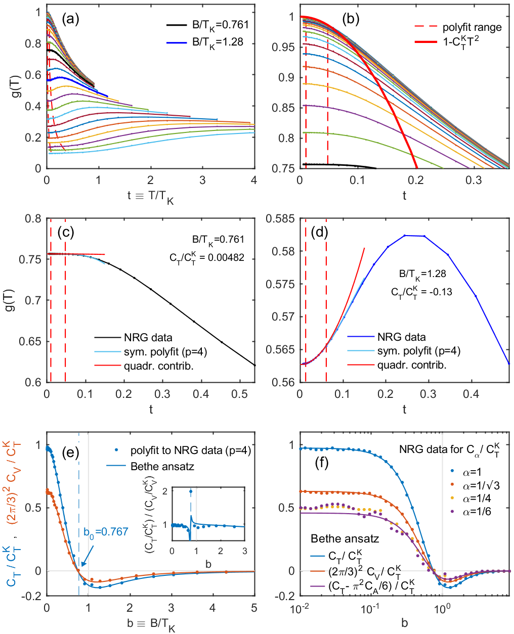
Figure 8: NRG analysis of the transport coefficients $C_{T}$ and $C_{V}$. (a) The linear conductance, $g(T)=g_{\alpha=1}(T)$, plotted as function of $t\equiv T/T_{K}$, for a uniform logarithmic grid of magnetic fields around $T_{K}$ [cf. data points in panels (e-f)]. The red vertical dashed lines indicate the fitting range used to extract curvatures. (b) Zoom into the low-temperature regime of (a). The thick red line shows the FL prediction at zero field, $1-C_{T}^{K}T^{2}$. (c,d) Illustration of the fit quality for two curves from (a) for magnetic fields around $C_{T}\approx 0$ and around the largest negative value of $C_{T}$, respectively. (e) $C_{1}=C_{T}$ (blue) and $C_{1/\sqrt{3}}=(2\pi/3)^{2}C_{V}$ (red), normalized by $C_{T}^{K}$ and plotted versus $B/T_{K}$. The agreement with the corresponding FL predictions (solid lines in matching color) from the main text is excellent. Inset: the ratio $C_{T}/C_{T}^{K}$ over $C_{V}/C_{V}^{K}$, showing that both have the same limits for $B/T_{K}\ll$ and $\gg 1$. (f) $C_{\alpha}/C_{T}^{K}$ for several values of $\alpha$, plotted on a log scale as function of $B/T_{K}$. The data for $\alpha=1$ and $1/\sqrt{3}$ replicate those from from (e) for $C_{T}$ and $C_{V}$. For comparison, solid lines show Bethe ansatz data. NRG parameters: $\Lambda=2$, $z$-averaged at $n_{z}=8$; truncation by number of multipets, with $N^{\ast}_{\mathrm{kept}}=1060$ (corresponding to $6944$ states).

D.2 Numerical results

Our NRG calculations were performed for the single-impurity Anderson model with a box-shaped density of states with half-bandwidth $D=1$, which thus sets the unit of energy unless specified otherwise. For the results shown in Fig. 8, we used a hybridization strength $\Delta=10^{-3}$, $U/\Delta=5$, $\epsilon_{d}=-U/2$, resulting in a Kondo temperature of $T_{K}=2.990\cdot 10^{-4}$. Since both $U$ and $\Gamma$ are much smaller than the bandwidth, and the local dynamics is cut off by the energy scale $U$, the parameter regime analyzed essentially is equivalent Hanl et al. (2014) to an infinite bandwidth scenario as considered in the main text.

Our NRG results for the temperature-dependent linear conductance, $g(T)=g_{\alpha=1}(T)$, are shown in Fig. 8(a), for a fine-grained set of $B$-values uniformly distributed around $T_{K}$ on a logarithmic grid. To determine the Fermi liquid coefficient $C_{T}=C_{\alpha=1}$ for a given field, the curvature of the corresponding curve must be extracted in the regime $t\equiv T/T_{K}\ll 1$. On the other hand, $t$ must be sufficiently large that the temperature-dependent variation in $g(T)$ exceeds the NRG resolution (typically, $\delta g\gtrsim 10^{-3}$). In practice, we constrain the fitting interval to $t\in[0.01,0.05]\times\max(T_{K},B)$ [vertical dashed lines in Figs. 8(b-d)]. Since we use a fine-grained logarithmic grid for $t$, cutting out $t<0.01$ is also required to avoid a bias of the fit towards a dense set of data points at $t=0$. We perform a symmetrized $(p=4)$-th order polynomial fit, by also including the mirror image $t\to-t$ of the data. This way, only even polynomial coefficients are non-zero.

Two exemplary fits are shown in Figs. 8(c,d). In panel (c), $C_{T}\approx 0$, indicating that the field is close to the value $B_{T}$ where the curvature $C_{T}$ changes sign. In contrast, Fig. 8(d) analyzes the conductance data for the magnetic field where the upward curvature in the conductance is maximal [this corresponds to the minimum of $c_{T}$ in Fig. 8(e)]. Both panels (c) and (d) show that $g(T)$ deviates significantly from the quadratic regime already for $t\simeq 0.1$. Hence smaller $t$ is required for the fit (here we use $t\leq 0.05$) while already also allowing for quartic corrections. Moreover, note that $g_{\alpha}(T)$ varies by $\lesssim 0.5\%$ over the fitting interval, illustrating that an accurate determination of the curvature requires $g_{\alpha}(T)$ to be known with an accuracy of order $\lesssim 0.1\%$.

Fig. 8(e) shows the curvatures $C_{T}$ and $(2\pi/3)^{2}C_{V}$ extracted from all the curves in panel (a), normalized by $C_{T}^{K}$ and plotted as dots, as functions of $B/T_{K}$. The NRG results are in very good agreement with the FL predictions (Bethe ansatz data, solid lines, replotted from Fig. 3 of main text). For the specific value $U/\Delta=5$ used in this plot, the field at which $C_{T}$ vanishes, as obtained by interpolation from the discrete set of NRG data points, is $B_{T}/T_{K}=0.767$. This agrees to within about 1% with the FL prediction. Panel (f) replots the data from (e) on a log-$x$ scale, showing good agreement down to the smallest magnetic fields.

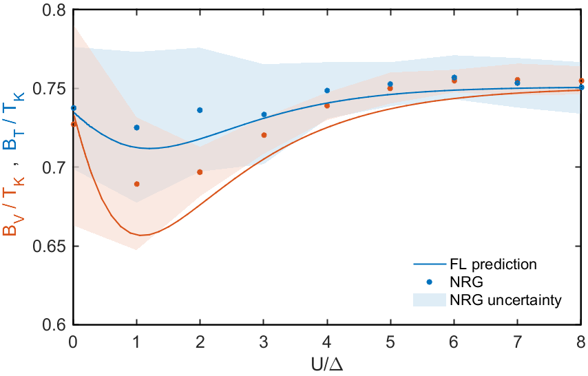
Figure 9: Comparison of results from NRG and FL theory for $B_{T}$ and $B_{V}$, corresponding to Fig. 3 of the main text. The color-matched shaded regions are estimates for the error margins, simply based on matlab polyfit confidence intervals. NRG parameters: $\Delta=0.001$, $\Lambda=2$, with $N^{\ast}_{\mathrm{kept}}\leq 1244$ multiplets ($8176$ states), $z$-averaged at $n_{z}=4$.

We have repeated the above analysis for a range of interaction strengths to extract $B_{T}$ and $B_{V}$ as functions of $U/\Delta$. The results are shown in Fig. 9. The NRG results are consistent with the FL predictions within the indicated simple error estimates. Note that the error estimates increase with decreasing $U/\Delta$, because this causes the Kondo peak to become broader, making it more difficult to accurately extract curvature coefficients. The fact that the error estimates are quite sizeable, varying between 3% and 12%, reflects the challenge of extracting curvatures from an energy window that necessarily has to be very small to satisfy the requirement $\varepsilon,T\ll T_{K}$.

We conclude this subsection with a technical remark. Since $\widetilde{C}_{\!A}=\frac{6}{\pi^{2}}C_{0}$ and $C_{\!A}=\frac{6}{\pi^{2}}(C_{1}-C_{0})$, one may attempt to compute these coefficients via $C_{1}$ and $C_{0}$. Note, though, that $C_{0}$ can not be extracted by simply using $\alpha\to 0^{+}$, because the discrete NRG data looses spectral support at energies below $\sim T/10$ (see Fig. 2(b) of Weichselbaum and von Delft (2007)). Therefore, when the peaked function $-df_{\alpha}(\varepsilon)/d\varepsilon$ becomes too narrow as $\alpha$ is decreased, the numerically determined $g_{\alpha}(T)$ first becomes a noisy function of $T$, and eventually drops to zero for very small $\alpha$. Indeed, Fig. 8(f), which displays curves of $C_{\alpha}/C_{T}^{K}$ versus $B/T_{K}$ for several values $\alpha\in[0,1]$, shows that these curves become more ‘noisy’ as $\alpha$ is decreased. The increase in noise in spectral resolution seen at $\alpha=1/4$ becomes large very quickly for $\alpha<0.25$.

$C_{0}$ can nevertheless be determined to fairly good accuracy by noting that the overall shape of the curves in Fig. 8(f) essentially stops changing for $\alpha<0.25$. Hence $C_{0.25}$ may be viewed as an approximation for $C_{0}$. Indeed, its low-field limit, $C_{0.25}\simeq C_{T}^{K}/2$, is consistent with the value expected for $C^{K}_{0}=C_{T}^{K}/2$. For comparison, Fig. 8(f) also shows the Bethe ansatz data for $C_{0}=C_{1}-\tfrac{\pi^{2}}{6}C_{\!A}=C_{T}-\tfrac{\pi^{2}}{6}C_{\!A}.$ The agreement with the NRG data is within the increased level of spectral noise of the NRG data.

D.3 Remarks on our previous NRG results

We conclude this appendix with a brief discussion of why, in retrospect, the NRG results presented in a previous version of this paper, Filippone et al. (2017), were unreliable. There are two main reasons: first, they were obtained using only 1024 states (here we use 6944), and no $z$-averaging (here we use $n_{z}=8$). Hence they did not achieve the $\mathcal{O}(0.1\%)$ accuracy needed for $g_{\alpha}(T)$ to allow an accurate determination of its curvature. Second, we had attempted to extract the curvature coefficients $C_{\!A}$ and $\widetilde{C}_{\!A}$ by following a strategy described in section IV.D of Ref. Hanl et al. (2014). However, that strategy had been devised only to determine $C_{\!A}$ at $T{=}0$. In retrospect, our attempt to generalize it to determine both $C_{\!A}$ and $\widetilde{C}_{\!A}$ at nonzero $T$ had been flawed, which is why we now instead use $C_{1}$ and $C_{1/\sqrt{3}}$ to determine $C_{T}$ and $C_{V}$, as described above.

Appendix E Perturbation results in the $\varepsilon_{d}\gg\Delta$ limit.

The FL coefficients needed to derive the spectral coefficients $\tilde{c}_{A},c_{A}$ and transport coefficients $c_{V},c_{T}$, depend on the zero-temperature dot occupation functions $n_{d\sigma}$ and their derivatives with respect to the level energy ${\varepsilon_{d}}$ and magnetic field $B$. Deep in the empty-orbital regime, where $\varepsilon_{d}\gg\Delta$, the leading corrections to the noninteracting occupations,

$$n^{0}_{d\uparrow}= \tfrac{1}{2}-\tfrac{1}{\pi}\,{\rm arctan}\left[\left(\varepsilon_{d}-\tfrac{1}{2}B\right)/\Delta\right],$$ (79)

can be computed perturbatively in the dot-lead hybridization, using the spin-down state of the dot as intermediate state (see also Ref. Filippone et al., 2013), with the result

$$n_{d\uparrow}= n^{0}_{d\uparrow}-\frac{\Delta}{\pi}\frac{Un_{d\uparrow}^{0}(1-n_{d\uparrow}^{0})}{(U+\varepsilon_{d}+\frac{1}{2}B)(\varepsilon_{d}+\frac{1}{2}B)},$$ (80a)

$$n_{d\downarrow}= \frac{\Delta}{\pi}\left(\frac{1-n_{d\uparrow}^{0}}{\varepsilon_{d}+\frac{1}{2}B}+\frac{n_{d\uparrow}^{0}}{\varepsilon_{d}+U+\frac{1}{2}B}\right).$$ (80b)

All FL parameters can be straightforwardly computed from these expressions using Eqs. (12) and (13). To compare with the numerical results in Fig. 7, we substitute $\varepsilon_{d}\to{\tilde{\varepsilon}_{d}}$ [cf. Eq. (42)] in the final result for $c_{V}$.

References

- Goldhaber-Gordon et al. (1998) D. Goldhaber-Gordon, H. Shtrikman, D. Mahalu, D. Abusch-Magder, U. Meirav, and M. Kastner, Nature 391, 156 (1998).
- Kogan et al. (2004) A. Kogan, S. Amasha, D. Goldhaber-Gordon, G. Granger, M. A. Kastner, and H. Shtrikman, Phys. Rev. Lett. 93, 166602 (2004).
- Houck et al. (2005) A. A. Houck, J. Labaziewicz, E. K. Chan, J. A. Folk, and I. L. Chuang, Nano Letters 5, 1685 (2005).
- Amasha et al. (2005) S. Amasha, I. J. Gelfand, M. A. Kastner, and A. Kogan, Phys. Rev. B 72, 045308 (2005).
- Quay et al. (2007) C. H. L. Quay, J. Cumings, S. J. Gamble, R. dePicciotto, H. Kataura, and D. Goldhaber-Gordon, Phys. Rev. B 76, 245311 (2007).
- Jespersen et al. (2006) T. S. Jespersen, M. Aagesen, C. Sørensen, P. E. Lindelof, and J. Nygård, Phys. Rev. B 74, 233304 (2006).
- Liu et al. (2009) T.-M. Liu, B. Hemingway, A. Kogan, S. Herbert, and M. Melloch, Phys. Rev. Lett. 103, 026803 (2009).
- Glazman and Raikh (1988) L. Glazman and M. Raikh, JETP Lett. 47, 452 (1988).
- Ng and Lee (1988) T. K. Ng and P. A. Lee, Phys. Rev. Lett. 61, 1768 (1988).
- Glazman and Pustilnik (2003) L. Glazman and M. Pustilnik, in New Directions in Mesoscopic Physics (Towards Nanoscience), edited by R. Fazio, V. Gantmakher, and Y. Imry (Kluwer, Dordrecht, 2003).
- Glazman and Pustilnik (2004) L. Glazman and M. Pustilnik, J. Phys.: Condens. Matter 16, R513 (2004).
- Chang and Chen (2009) A. M. Chang and J. C. Chen, Rep. Prog. Phys. 72, 096501 (2009).
- Rosch et al. (2003) A. Rosch, J. Paaske, J. Kroha, and P. Wölfle, Phys. Rev. Lett. 90, 076804 (2003).
- Kehrein (2005) S. Kehrein, Phys. Rev. Lett. 95, 056602 (2005).
- Doyon and Andrei (2006) B. Doyon and N. Andrei, Phys. Rev. B 73, 245326 (2006).
- Dias da Silva et al. (2008) L. G. G. V. Dias da Silva, F. Heidrich-Meisner, A. E. Feiguin, C. A. Busser, G. B. Martins, E. V. Anda, and E. Dagotto, Phys. Rev. B 78, 195317 (2008).
- Schoeller (2009) H. Schoeller, The European Physical Journal Special Topics 168, 179 (2009).
- Eckel et al. (2010) J. Eckel, F. Heidrich-Meisner, S. Jakobs, M. Thorwart, M. Pletyukhov, and R. Egger, New. J. Phys. 12, 043042 (2010).
- Moca et al. (2011) C. P. Moca, P. Simon, C. H. Chung, and G. Zaránd, Phys. Rev. B 83, 201303 (2011).
- Gezzi et al. (2007) R. Gezzi, T. Pruschke, and V. Meden, Phys. Rev. B 75, 045324 (2007).
- Metzner et al. (2012) W. Metzner, M. Salmhofer, C. Honerkamp, V. Meden, and K. Schönhammer, Rev. Mod. Phys. 84, 299 (2012).
- Pletyukhov and Schoeller (2012) M. Pletyukhov and H. Schoeller, Phys. Rev. Lett. 108, 260601 (2012).
- Smirnov and Grifoni (2013) S. Smirnov and M. Grifoni, Phys. Rev. B 87, 121302 (2013).
- Schiller and Hershfield (1998) A. Schiller and S. Hershfield, Phys. Rev. B 58, 14978 (1998).
- Boulat and Saleur (2008) E. Boulat and H. Saleur, Phys. Rev. B 77, 033409 (2008).
- Anders and Schiller (2005) F. B. Anders and A. Schiller, Phys. Rev. Lett. 95, 196801 (2005).
- Anders (2008) F. B. Anders, Phys. Rev. Lett. 101, 066804 (2008).
- Cohen et al. (2014) G. Cohen, E. Gull, D. R. Reichman, and A. J. Millis, Phys. Rev. Lett. 112, 146802 (2014).
- Dorda et al. (2015) A. Dorda, M. Ganahl, H. G. Evertz, W. von der Linden, and E. Arrigoni, Phys. Rev. B 92, 125145 (2015).
- Note (1) An attempt in this direction was made in Ref. Hewson et al. (2005) for the symmetric Anderson model, using renormalized perturbation theory. However their results disagree with the results presented here (see the end of Section 5).
- Hewson et al. (2005) A. C. Hewson, J. Bauer, and A. Oguri, J. Phys.: Condens. Matter 17, 5413 (2005).
- Nozières (1974a) P. Nozières, J. Low Temp. Phys. 17, 31 (1974a).
- Nozières (1974b) P. Nozières, in Proceedings of the 14th International Conference on Low Temperature Physics, Vol. 5, edited by M. Krasius and M. Vuorio (North Holland, Amsterdam, 1974) pp. 339-374.
- Nozières (1978) P. Nozières, J. Physique 39, 1117 (1978).
- Yosida and Yamada (1970) K. Yosida and K. Yamada, Prog. Theor. Phys. 46, 244 (1970).
- Yamada (1975a) K. Yamada, Prog. Theor. Phys. 53, 970 (1975a).
- Yosida and Yamada (1975) K. Yosida and K. Yamada, Prog. of Theor. Phys. 53, 1286 (1975).
- Yamada (1975b) K. Yamada, Prog. Theor. Phys. 54, 316 (1975b).
- Yoshimori (1976) A. Yoshimori, Prog. Theor. Phys. 55, 67 (1976).
- Mihály and Zawadowski (1978) L. Mihály and A. Zawadowski, J. Phys. (Paris) Lett. 39, 483 (1978).
- Sakano et al. (2011a) R. Sakano, T. Fujii, and A. Oguri, Phys. Rev. B 83, 075440 (2011a).
- Sakano et al. (2011b) R. Sakano, A. Oguri, T. Kato, and S. Tarucha, Phys. Rev. B 83, 241301 (2011b).
- Hörig et al. (2014) C. B. M. Hörig, C. Mora, and D. Schuricht, Phys. Rev. B 89, 165411 (2014).
- Hanl et al. (2014) M. Hanl, A. Weichselbaum, J. von Delft, and M. Kiselev, Phys. Rev. B 89, 195131 (2014).
- Hewson (1993a) A. C. Hewson, The Kondo Problem to Heavy Fermions (Cambridge University Press, Cambridge, 1993).
- Hewson (2005) A. C. Hewson, J. Phys. Soc. Jpn. 74, 8 (2005).
- Hewson (1993b) A. C. Hewson, Phys. Rev. Lett. 70, 4007 (1993b).
- Hewson (1993c) A. C. Hewson, J. Phys.: Condens. Matter 5, 6277 (1993c).
- Hewson (1994) A. C. Hewson, Adv. Phys. 43, 543 (1994).
- Hewson (2001) A. C. Hewson, J. Phys.: Condens. Matter 13, 10011 (2001).
- Hewson et al. (2004) A. C. Hewson, A. Oguri, and D. Meyer, Eur. Phys. J. B 40, 177 (2004).
- Hewson et al. (2006) A. C. Hewson, J. Bauer, and W. Koller, Phys. Rev. B 73, 045117 (2006).
- Bauer and Hewson (2007) J. Bauer and A. C. Hewson, Phys. Rev. B 76, 035119 (2007).
- Edwards and Hewson (2011) K. Edwards and A. C. Hewson, J. Phys.: Condens. Matter 23, 045601 (2011).
- Edwards et al. (2013) K. Edwards, A. C. Hewson, and V. Pandis, Phys. Rev. B 87, 165128 (2013).
- Pandis and Hewson (2015) V. Pandis and A. C. Hewson, Phys. Rev. B 92, 115131 (2015).
- Hamad et al. (2015) I. J. Hamad, C. Gazza, J. A. Andrade, A. A. Aligia, P. S. Cornaglia, and P. Roura-Bas, Phys. Rev. B 92, 195113 (2015).
- Hewson (2006) A. C. Hewson, J. Phys.: Condens. Matter 18, 1815 (2006).
- Lesage and Saleur (1999a) F. Lesage and H. Saleur, Phys. Rev. Lett. 82, 4540 (1999a).
- Lesage and Saleur (1999b) F. Lesage and H. Saleur, Nucl. Phys. B 546, 585 (1999b).
- Freton and Boulat (2014) L. Freton and E. Boulat, Phys. Rev. Lett. 112, 216802 (2014).
- Mora et al. (2015) C. Mora, C. P. Moca, J. von Delft, and G. Zaránd, Phys. Rev. B 92, 075120 (2015).
- Oguri (2001) A. Oguri, Phys. Rev. B 64, 153305 (2001).
- Glazman and Pustilnik (2005) L. Glazman and M. Pustilnik, in Nanophysics: Coherence and Transport, edited by H. et al.. Bouchiat (Elsevier, Amsterdam, 2005) pp. 427–478, cond-mat/0501007.
- Sela et al. (2006) E. Sela, Y. Oreg, F. von Oppen, and J. Koch, Phys. Rev. Lett. 97, 086601 (2006).
- Golub (2006) A. Golub, Phys. Rev. B 73, 233310 (2006).
- Gogolin and Komnik (2006) A. O. Gogolin and A. Komnik, Phys. Rev. Lett. 97, 016602 (2006).
- Mora et al. (2008) C. Mora, X. Leyronas, and N. Regnault, Phys. Rev. Lett. 100, 036604 (2008).
- Mora (2009) C. Mora, Phys. Rev. B 80, 125304 (2009).
- Mora et al. (2009) C. Mora, P. Vitushinsky, X. Leyronas, A. A. Clerk, and K. Le Hur, Phys. Rev. B 80, 155322 (2009).
- Vitushinsky et al. (2008) P. Vitushinsky, A. A. Clerk, and K. Le Hur, Phys. Rev. Lett. 100, 036603 (2008).
- Fujii (2010) T. Fujii, J. Phys. Soc. Jpn. 79 (2010).
- Wilson (1975) K. G. Wilson, Rev. Mod. Phys. 47, 773 (1975).
- Bulla et al. (2008) R. Bulla, T. A. Costi, and T. Pruschke, Rev. Mod. Phys. 80, 395 (2008).
- Weichselbaum (2012a) A. Weichselbaum, Phys. Rev. B 86, 245124 (2012a).
- Garst et al. (2005) M. Garst, P. Wölfle, L. Borda, J. von Delft, and L. Glazman, Phys. Rev. B 72, 205125 (2005).
- Filippone et al. (2017) M. Filippone, C. P. Moca, J. von Delft, and C. Mora, Phys. Rev. B 95, 165404 (2017), arXiv:1609.06165v1 [cond-mat.mes-hall].
- Oguri and Hewson (2018a) A. Oguri and A. C. Hewson, Phys. Rev. Lett. 120, 126802 (2018a).
- Oguri and Hewson (2018b) A. Oguri and A. C. Hewson, Phys. Rev. B 97, 045406 (2018b).
- Oguri and Hewson (2018c) A. Oguri and A. C. Hewson, Phys. Rev. B 97, 035435 (2018c).
- Note (2) In the non-universal case of a finite bandwidth, the Fermi liquid relations that we derive are no longer strictly valid. Nevertheless, the corrections to our predictions are expected to be small with the ratio of the maximum of , , and over the bandwidth of the model.
- Affleck and Ludwig (1991) I. Affleck and A. W. W. Ludwig, Nucl. Phys. B 360, 641 (1991).
- Affleck and Ludwig (1993) I. Affleck and A. W. W. Ludwig, Phys. Rev. B 48, 7297 (1993).
- Tsvelick and Wiegmann (1983a) A. Tsvelick and P. Wiegmann, Adv. Phys. 32, 453 (1983a).
- Note (3) See Supplemental Material, where the Bethe Ansatz expressions used here are reviewed.
- Haldane (1978a) F. D. M. Haldane, Phys. Rev. Lett. 40, 416 (1978a).
- Haldane (1978b) F. D. M. Haldane, J. Phys. C: Solid State Phys. 11, 5015 (1978b).
- Meir and Wingreen (1992) Y. Meir and N. S. Wingreen, Phys. Rev. Lett. 68, 2512 (1992).
- Blanter and Büttiker (2000) Y. M. Blanter and M. Büttiker, Phys. Rep. 336, 1 (2000).
- Kamenev and Levchenko (2009) A. Kamenev and A. Levchenko, Adv. Phys. 58, 197 (2009).
- Note (4) In Ref. Filippone et al. (2017), the last term in Eq. (25\@@italiccorr) erroneously contained a factor instead of . Consequently most subsequent expressions for were incorrect. For example, Eq. (27b\@@italiccorr) contained an instead of , and Eq. (32b\@@italiccorr) an incorrect sign, minus instead of plus, in front of the term. This lead to the wrong conclusion that in the Kondo limit and remain positive for large fields – insteady, they turn negative; and that “the conductance retains a (very weak) zero-bias maximum even for strong magnetic fields” – instead, the zero-bias maximum turns into a minimum at a field of order .
- Note (5) Expression (24b\@@italiccorr) for stems from the quadratic contribution of the term in to the quasi-particle self-energy. Its contribution is well known in an equilibrium context Nozières (1974a); *nozieres1974b; *nozieres1978; Affleck and Ludwig (1993). We obtained its contribution as follows. Since , and all characterize the phase space available for inelastically scattering a quasiparticle having energy , their contributions all have the same general form, differing only by numerical prefactors. We deduced that of to be by inserting a general low-energy expansion for into (23\@@italiccorr) for , expanding the latter in the form (29\@@italiccorr) and equating the resulting expression for to the quantity found in Ref. Mora et al. (2015) by a direct calculation of the current. The resulting combination in Eq. (24b) for is consistent with that reported in Eq. (43) of Ref. Oguri (2005) for the imaginary part of the local self-energy in renormalized perturbation theory.
- Note (6) The numerical prefactor for was chosen to ensure that in the Kondo limit at zero field, see Eq. (34a).
- Aligia (2012) A. A. Aligia, J. Phys.: Condens. Matter 24, 015306 (2012).
- Muñoz et al. (2013) E. Muñoz, C. J. Bolech, and S. Kirchner, Phys. Rev. Lett. 110, 016601 (2013).
- Aligia (2014) A. A. Aligia, Phys. Rev. B 89, 125405 (2014).
- Costi (2000) T. A. Costi, Phys. Rev. Lett. 85, 1504 (2000).
- Wright et al. (2011) C. J. Wright, M. R. Galpin, and D. E. Logan, Phys. Rev. B 84, 115308 (2011).
- Zitko et al. (2009) R. Zitko, R. Peters, and T. Pruschke, New Journal of Physics 11, 053003 (2009).
- Moore and Wen (2000) J. E. Moore and X.-G. Wen, Phys. Rev. Lett. 85, 1722 (2000).
- Rosch et al. (2005) A. Rosch, J. Paaske, J. Kroha, and P. Wölfle, Journal of the Physical Society of Japan 74, 118 (2005).
- Weichselbaum et al. (2009) A. Weichselbaum, F. Verstraete, U. Schollwöck, J. I. Cirac, and J. von Delft, Phys. Rev. B 80, 165117 (2009).
- Hewson (2016) A. C. Hewson, private communication (2016).
- Wiegmann (1980) P. Wiegmann, Physics Letters A 80, 163 (1980).
- Kawakami and Okiji (1982) N. Kawakami and A. Okiji, J. Phys. Soc. Jpn. 51, 2043 (1982).
- Wiegmann and Tsvelick (1983) P. Wiegmann and A. Tsvelick, J. Phys. C 16, 2281 (1983).
- Tsvelick and Wiegmann (1983b) A. Tsvelick and P. Wiegmann, J. Phys. C 16, 2321 (1983b).
- Grabert and Devoret (2013) H. Grabert and M. H. Devoret, Single charge tunneling: Coulomb blockade phenomena in nanostructures, Vol. 294 (Springer Science & Business Media, 2013).
- Note (7) Eq. (42\@@italiccorr) is derived from the seminal expression of the renormalized level provided by Haldane in Ref. Haldane (1978a), , in which is the energy scale at which the orbital energy renormalization starts, namely , and the energy scale in which the renormalization stops, i.e. . Notice that this formula for applies within a regime different from the mixed valence regime; in the latter, , hence is the lowest energy scale in the problem and the renormalization stops at . For the data sets presented in Fig. 7(a), is still comparable to (but somewhat larger than) the hybridization energy and the charging energy .
- Filippone et al. (2013) M. Filippone, K. Le Hur, and C. Mora, Phys. Rev. B 88, 045302 (2013).
- Oguri and Hewson (2017) A. Oguri and A. C. Hewson, private communication (2017).
- Note (8) Up to terms which can be written as total derivatives in the action formalism, see Supplementary Note S-IV in Ref. \rev@citealpmora2015.
- Weichselbaum and von Delft (2007) A. Weichselbaum and J. von Delft, Phys. Rev. Lett. 99, 076402 (2007).
- Weichselbaum (2012b) A. Weichselbaum, Annals of Physics 327, 2972 (2012b).
- Oliveira (1992) L. N. Oliveira, Braz. J. Phys 22, 155 (1992).
- Zitko Žitko and Pruschke (2009) R. Zitko Žitko and T. Pruschke, Phys. Rev. B 79, 085106 (2009).
- Lee and Weichselbaum (2016) S.-S. B. Lee and A. Weichselbaum, Phys. Rev. B 94, 235127 (2016).
- Oguri (2005) A. Oguri, J. Phys. Soc. Jpn. 74, 110 (2005).