Probing the scale invariance of the inflationary power spectrum in expanding quasi-two-dimensional dipolar condensates

Abstract

We consider an analogue de Sitter cosmos in an expanding quasi-two-dimensional Bose-Einstein condensate with dominant dipole-dipole interactions between the atoms or molecules in the ultracold gas. It is demonstrated that a hallmark signature of inflationary cosmology, the scale invariance of the power spectrum of inflaton field correlations, experiences strong modifications when, at the initial stage of expansion, the excitation spectrum displays a roton minimum. Dipolar quantum gases thus furnish a viable laboratory tool to experimentally investigate, with well-defined and controllable initial conditions, whether primordial oscillation spectra deviating from Lorentz invariance at trans-Planckian momenta violate standard predictions of inflationary cosmology.

The hypothesis of a rapid initial expansion of the cosmos in the inflationary scenario Guth (1981); Linde (1982); Mukhanov (2005) resolved many vexing cosmological questions plaguing other theories, such as the observed flatness and homogeneity of the universe, as well as the nonexistence of monopoles. However the resolution of these issues comes at the price of creating another potential problem Martin and Brandenberger (2001): Generally the period of inflation lasts so long that, at the beginning of the inflationary period, the physical wavelengths of comoving scales which correspond to the present large-scale structure of the universe were smaller than the Planck length. Thus necessarily trans-Planckian energies become involved, for which the physics is at present speculative. Similar issues regarding kinematical phenomena for quantum fields propagating on a fixed curved spacetime arise when tracing back Hawking radiation emission all the way down to the black hole horizon Unruh (1995); Corley and Jacobson (1996); Unruh and Schützhold (2005); Leonhardt and Robertson (2012).

The analogue gravity program Unruh (1981); Visser (1998a); Volovik (2009); Barceló et al. (2011) has been successfully theoretically implemented in ultracold matter for various cosmological phenomena, e.g., inflaton quantum fluctuations Fischer and Schützhold (2004); Uhlmann et al. (2005), the Gibbons-Hawking effect Fedichev and Fischer (2003), cosmological particle production Barceló et al. (2003a); Fedichev and Fischer (2004); Weinfurtner et al. (2009), the cosmological constant problem Volovik (2009); Finazzi et al. (2012); Jannes and Volovik (2012), or false vacuum decay Fialko et al. (2015). Importantly, recent experimental advances have allowed for groundbreaking observations of analogues of cosmological particle production, Sakharov oscillations, black hole lasers, and Hawking radiation Jaskula et al. (2012); Hung et al. (2013); Steinhauer (2014); Boiron et al. (2015); Steinhauer (2016). In the near future, these experiments hold promise to realize experimental cosmology: A quantum simulation of inflation with reproducible initial conditions distinct from the current purely observational cosmology of a pregiven state of the universe. Furthermore, a major original motivation of analogue gravity, so far not experimentally investigated, is to probe consequences of trans-Planckian physics in a microscopically well understood setup in a regime inaccessible for quantum fields in the presence of strong real (Einsteinian or other) gravity. We here propose to realize this aim with dipolar Bose-Einstein condensates (BECs), addressing the trans-Planckian problem of inflationary cosmology.

Going beyond contact interactions (in field theory language $\phi^{4}$), magnetic dipole-dipole interaction (DDI) dominated condensates with chromium Lahaye et al. (2007), dysprosium Lu et al. (2011), and erbium Aikawa et al. (2012) atoms have been created, and the future realization of electrically dipolar BECs Quéméner and Julienne (2012) will offer even greater flexibility in controlling the ratio of dipolar and contact interactions. The excitation spectrum of DDI-dominated BECs displays a roton minimum Santos et al. (2003); Fischer (2006); Ronen et al. (2007), and roton-induced dynamical effects are being experimentally investigated Kadau et al. (2016); Ferrier-Barbut et al. (2016). In addition, the significant progress in probing correlation functions to increasing accuracy Hung et al. (2013); Hodgman et al. (2011) pave the way for an exploration of the intricate many-body correlations due to the DDI.

For certain classes of inflaton dispersion relations, displaying deviations from Lorentz invariance at trans-Planckian scales, the predictions of inflation, in particular the scale invariance of the power spectrum (SIPS) of inflaton field correlations, remain robust, while for others, they change significantly, cf., e.g., Niemeyer and Parentani (2001); Starobinsky (2001); Brandenberger and Martin (2001, 2001, 2013); Zhu et al. (2014). We will show that dipolar BECs, possessing trans-Planckian spectra leading to strong departures from Lorentz invariance, yield significant changes of the standard inflationary prediction of SIPS. To the best of our knowledge, this represents the first example within analogue gravity where violations of SIPS can become experimentally manifest.

We start with the Lagrangian density of a Bose gas comprising atoms or molecules of mass $m$,

$$\mathcal{L} =\frac{i\hbar}{2}\bigl{(}\Psi^{*}\partial_{t}{\Psi}-\partial_{t}{\Psi}^{*}\Psi\bigr{)}-\frac{\hbar^{2}}{2m}|\nabla\Psi|^{2}-V_{\mathrm{ext}}|\Psi|^{2}$$

$$\quad-\frac{1}{2}|\Psi|^{2}\int d^{3}\mathbf{R}^{\prime}\,V_{\mathrm{int}}(\mathbf{R}-\mathbf{R}^{\prime})|\Psi(\mathbf{R}^{\prime})|^{2},$$ (1)

where $\mathbf{R}=(\mathbf{r},z)$ are spatial 3D coordinates. The trapping potential is $V_{\mathrm{ext}}(\mathbf{R},t)=m\omega^{2}\mathbf{r}^{2}/2+m\omega_{z}^{2}z^{2}/2,$ where $\omega$ and $\omega_{z}$ can be chosen functions of time. The gas is strongly confined in $z$-direction, with aspect ratio $\kappa=\omega_{z}/\omega\gg 1$ over the whole time evolution. The interaction reads $V_{\mathrm{int}}(\mathbf{R}-\mathbf{R}^{\prime})=g_{c}\delta^{(3)}(\mathbf{R}-\mathbf{R}^{\prime})+V_{\mathrm{dd}}(\mathbf{R}-\mathbf{R}^{\prime}),$ where $g_{c}$ is the contact interaction coupling, and $V_{\mathrm{dd}}(\mathbf{R})=3g_{d}[(1-3z^{2}/|\mathbf{R}|^{2})/|\mathbf{R}|^{3}]/4\pi$ for dipoles polarized perpendicular to the plane. We have a scaling law $V_{\rm int}(\Lambda\mathbf{R})=\Lambda^{\alpha}V_{\rm int}(\mathbf{R})$ Gritsev et al. (2010) for a combined 3D contact and dipolar potential with $\alpha=-3$. Note that the scaling equation (4) below is thus 3D. To ensure stability in the DDI dominated regime Fischer (2006), we impose the system to stay sufficiently close to the quasi-2D regime during expansion. We integrate out the $z$ dependence by assuming a Gaussian, $\rho_{z}(z)=(\pi d_{z}^{2})^{-1/2}\exp\left[-{z^{2}}/{d_{z}^{2}}\right]$, where $d_{z}=b(t)d_{z,0}$, and $b(t)$ is the scale factor in Eq. (2) ren , where $d_{z,0}=\sqrt{\hbar/m\omega_{z,0}}$. The reduced contact coupling and lower-dimensional interaction are, respectively, then given by $g_{c}^{2\mathrm{D}}=g_{c}/\sqrt{2\pi}d_{z}$, $V_{\rm int}^{2\mathrm{D}}(\mathbf{r}-\mathbf{r}^{\prime})=\int dzdz^{\prime}\,V_{\rm int}(\mathbf{R}-\mathbf{R}^{\prime})\rho_{z}(z)\rho_{z}(z^{\prime})$ sup .

Employing the conventional scaling transformation to describe the evolution of the BEC upon changing the trapping or the coupling constants Kagan et al. (1996); Castin and Dum (1996); Gritsev et al. (2010),

$$\mathbf{x} :=\frac{\mathbf{r}}{b(t)},\;\;\quad\tau:=\int_{0}^{t}\frac{dt^{\prime}}{b^{2}(t^{\prime})},$$

$$\Psi(\mathbf{r},t) :=e^{i(mr^{2}/2\hbar)(\partial_{t}b/b)}\frac{\psi(\mathbf{x},\tau)}{b},$$ (2)

we obtain the nonlocal Gross-Pitaevskiǐ equation

$$i\hbar\partial_{\tau}\psi =-\frac{\hbar^{2}}{2m}\nabla_{x}^{2}\psi+f^{2}\biggl{(}\frac{m}{2}\omega_{0}^{2}x^{2}+g_{c,0}^{2\mathrm{D}}|\psi|^{2}$$

$$\quad+\int d^{2}\mathbf{x}^{\prime}\,V_{{\rm dd},0}^{2\mathrm{D}}(\mathbf{x}-\mathbf{x}^{\prime})|\psi(\mathbf{x}^{\prime})|^{2}\biggr{)}\psi.$$ (3)

We combined all remaining time dependences into a single factor $f=f(t)$, imposing Uhlmann (2009) [$b(0)=f(0)=1$]

$$f^{2}=\frac{b^{3}\partial^{2}_{t}b+b^{4}\omega^{2}(t)}{\omega_{0}^{2}}=\frac{g_{c}(t)}{g_{c,0}b}=\frac{g_{d}(t)}{g_{d,0}b}.$$ (4)

To separate off the effective contact interaction contribution $g_{0}^{\mathrm{eff}}$, we put $V_{\mathrm{int},0}^{2\mathrm{D}}(\mathbf{x}-\mathbf{x}^{\prime})=g_{c,0}^{2\mathrm{D}}\delta^{(2)}(\mathbf{x}-\mathbf{x}^{\prime})+V_{{\rm dd},0}^{2\mathrm{D}}(\mathbf{x}-\mathbf{x}^{\prime}):=g_{0}^{\mathrm{eff}}\delta^{(2)}(\mathbf{x}-\mathbf{x}^{\prime})+U_{0}^{2\mathrm{D}}(\mathbf{x}-\mathbf{x}^{\prime})$ sup .

The planar cloud size greatly exceeds the wavelengths of relevant Bogoliubov excitations in the plane. Especially near the center of cloud, density gradients are thus negligible, and we approximate the 2D comoving density $\rho_{0}\simeq$ const. The Bogoliubov equations for density and phase fluctuations read, with comoving momentum $\mathbf{k}$,

$$(\partial_{\tau}+i\mathbf{v}_{\rm com}\cdot\mathbf{k})\delta\rho_{\mathbf{k}} = \frac{\hbar\rho_{0}}{m}k^{2}\delta\phi_{\mathbf{k}},$$

$$(\partial_{\tau}+i\mathbf{v}_{\rm com}\cdot\mathbf{k})\delta\phi_{\mathbf{k}} = -\frac{f^{2}g_{0}^{\mathrm{eff}}}{\hbar}\mathcal{W}_{k}\delta\rho_{\mathbf{k}},$$ (5)

$$\mathcal{W}_{k}=\frac{\zeta^{2}}{4Af^{2}}+\frac{1}{g_{0}^{\mathrm{eff}}}{V}_{\mathrm{int},0}^{2\mathrm{D}}(\zeta), A=\frac{mc_{0}^{2}}{\hbar\omega_{z,0}},$$ (6)

and $c_{0}=\sqrt{{g_{0}^{\mathrm{eff}}\rho_{0}}/{m}}$. Furthermore, ${V}_{\mathrm{int},0}^{2\mathrm{D}}(\zeta)$ is the Fourier transform of $V_{\mathrm{int},0}^{2\mathrm{D}}$, with dimensionless $\zeta=kd_{z,0}$, and $\mathbf{v}_{\rm com}$ is the comoving frame velocity sup ; we assume it to be negligibly small in what follows, $\mathbf{v}_{\rm com}\simeq 0$.

Solving the second equation in (5) for $\delta\rho_{\mathbf{k}}$ and substituting into the first equation yields

$$\delta\ddot{\tilde{\phi}}_{k}+\biggl{(}2\frac{\dot{a}}{a}-\frac{\dot{\mathcal{W}}_{k}}{\mathcal{W}_{k}}\biggr{)}\delta\dot{\tilde{\phi}}_{k}+\biggl{(}\frac{c_{0}k}{a}\biggr{)}^{2}\mathcal{W}_{k}\delta\tilde{\phi}_{k}=0,$$ (7)

where overdot denotes $\tau$ derivatives, and we rescaled $\delta\tilde{\phi}=\Omega^{-1/2}\delta\phi,\;\Omega=c_{0}^{2}m^{2}/\hbar^{2}\rho_{0}$ for later convenience. We introduce the Friedmann-Robertson-Walker (FRW) cosmological scale factor by $a(t):=1/f(t)$, see below for a detailed discussion.

In an adiabatic regime Uhlmann (2009), momentarily ignoring time derivatives of $a$ and $\mathcal{W}_{k}$, the Bogoliubov dispersion is

$$\frac{\varepsilon^{2}}{(\hbar\omega_{z,0})^{2}}=\frac{A\zeta^{2}}{a^{2}}\left(1-\frac{3R}{2}\zeta w\left[\frac{\zeta}{\sqrt{2}}\right]\right)+\frac{\zeta^{4}}{4},$$ (8)

where the $w$ function $w(z)=\exp[z^{2}](1-{\rm erf}[z])$ contains the error function Fischer (2006); Abramowitz and Stegun (1970). The dimensionless parameter, $R=g_{d,0}/(d_{z,0}g_{0}^{\mathrm{eff}})={\sqrt{\pi/2}}/({1+g_{c,0}/2g_{d,0}})$, ranges from $R=0$ if $g_{d,0}/g_{c,0}\to 0$ to $R=\sqrt{\pi/2}$ for $g_{d,0}/g_{c,0}\to\infty$. In the latter DDI dominated case, the spectrum displays a “roton” minimum, which touches zero when $A$ is equal to the critical value $A_{c}=3.4454$, see Fig.1.

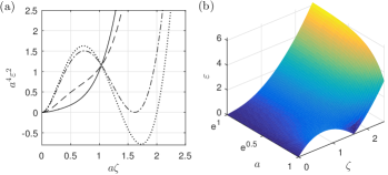
Figure 1: (a) Squared Bogoliubov excitation energy in units of $\hbar^{4}/4m^{2}d_{z,0}^{4}$, for DDI domination, $R=\sqrt{\pi/2}$. Counting from bottom to top at small $\zeta$, $A$ in (6) is $A_{c}/10,\;A_{\mathrm{min}},\;A_{c}$, and $1.1A_{c}$. For $A>A_{\mathrm{min}}=1.249$, the spectrum develops a roton minimum, and becomes unstable for $A>A_{c}=3.4454$. (b) Time evolution of the Bogoliubov spectrum in the course of expansion at criticality $A=A_{c}$. Initially, a roton minimum occurs, disappearing at late times.

In the long-wavelength limit, $\mathcal{W}_{k}\to 1$, and (7) becomes

$$\delta\ddot{\tilde{\phi}}_{k}+2\frac{\dot{a}}{a}\delta\dot{\tilde{\phi}}_{k}+\biggl{(}\frac{c_{0}k}{a}\biggr{)}^{2}\delta\tilde{\phi}_{k}=0.$$ (9)

The gravitational analogy can now be established by introducing the analogue space-time line element Barceló et al. (2011, 2003b); Fedichev and Fischer (2004)

$$ds^{2}=\Omega^{-2}(c_{0}^{2}d\tau^{2}-a^{2}d\mathbf{x}^{2}).$$ (10)

Then, (9) becomes the wave equation for a massless, minimally coupled free scalar field $\Box\delta\tilde{\phi}=(1/\sqrt{|\tilde{g}|})\partial_{\mu}(\sqrt{|\tilde{g}|}\tilde{g}^{\mu\nu}\partial_{\nu}\delta\tilde{\phi})=0$, in the (2+1)D FRW spacetime of Eq. (10) sup .

The simple possibility of $g_{c}(t)\propto g_{d}(t)\propto\exp[-2Ht]$ to realize an effective de Sitter (dark energy dominated) cosmos, $a=\exp[Ht]$, while having the advantage that the gas does not need to expand [$b(t)=1\,\forall\,t$ and thus $\tau:=t$], comes with the experimental difficulty that both couplings need to vary exponentially rapidly in lab time, see  Eqs. (2) and (4). While this is, in principle, possible Giovanazzi et al. (2002), also cf. Ref. Natu et al. (2014), we keep for the below discussion $g_{c}$ as well as $g_{d}$ constant; then $a^{2}(t)=b(t)$. For de Sitter expansion, $a(\tau)=1/f(\tau)=e^{H\tau}$, and thence in the lab,

$$b(t)=\sqrt{4Ht+1},\quad\omega^{2}(t)={\omega_{0}^{2}}/{b^{5}}+4H^{2}/b^{4}.$$ (11)

The radial condensate velocity then scales as $v=2Hr/b^{2}$ and the kinetic energy per particle, relative to $\omega_{z,0}$, as $A/b^{2}$. It thus decreases $\propto\omega_{z}$, ensuring proximity to the quasi-2D limit $\forall\,t$. The much slower (in comoving $\tau$ space) pre-de Sitter stage of cosmic expansion, $t<0$, is conceived such that it $\approx$ adiabatically leads to $\partial_{t}b(0)=2H$, and can be used to simulate as well the radiation- [$a(\tau)\propto\tau^{1/2}$] and matter-dominated [$a(\tau)\propto\tau^{2/3}$] eras Peacock (1999), by appropriately tuning $\omega(t)$ and/or $g_{c,d}(t)$.

It is noteworthy that with the (asymptotically square-root) expansion (11), Eq. (9) yields an analytical solution

$$\delta\tilde{\phi}_{k}(s)=s\sqrt{\frac{\pi\hbar VH}{4mc_{0}^{2}k^{2}}}\Bigl{[}J_{1}(s)+iY_{1}(s)\Bigr{]}:=h_{k}(s),$$ (12)

where the variable $s=(c_{0}/H)/(a/k)$ measures the ratio of Hubble radius to the cosmic expansion-rescaled wavelength, and $J_{1},Y_{1}$ are Bessel functions sup ; $s$ starts from $\infty$ and approaches zero when $\tau$ runs from $-\infty$ to $\infty$, that is when conformal time $\eta:=\int_{\infty}^{\tau}d\tau^{\prime}c_{0}/a(\tau^{\prime})$, for which $ds^{2}=a^{2}[d\eta^{2}-d\mathbf{x}^{2}]$, ranges from $-\infty$ to 0. The instantaneous vacuum corresponding to the basis $h_{k}(s)$ is the Bunch-Davies vacuum Bunch and Davies (1978), yielding an asymptotic Minkowski vacuum in the (formally) infinite past equivalent to the lab’s quasiparticle vacuum. It is assumed that the initial Bunch-Davies vacuum $\left|0\right>$ at $\eta=-c_{0}/H$ ($t=\tau=0$) is during the pre-de Sitter stage smoothly connected to this asymptotic vacuum. We emphasize that “cosmological” quasiparticles are measurable: In sup , we establish the equivalence of representations using cosmological comoving or scaling and lab frame Bogoliubov quasiparticles, also cf. Kurita et al. (2009); Barceló et al. (2010), and elaborate on the measurement process when the expansion is stopped.

The modes oscillate almost freely for $\eta\to-\infty$. At $k\eta=-1$ and horizon crossing, the mode freezes, leading to the standard theory of inhomogeneity or galaxy formation during inflation Mukhanov (2005). At late times, $s\rightarrow 0$, and the modes do effectively not evolve anymore. Fig. 2 shows the evolution of $kh_{k}$ as a function of $k\eta$; (b)$\sim$(d) illustrate the fact that when trans-Planckian defomation of the spectrum is included (see below), horizon crossing and mode freezing nontrivially still occur.

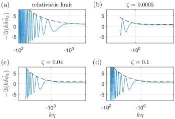
Figure 2: (a) Freezing process of the inflaton mode function $kh_{k}$ in units of $\sqrt{\hbar HV/\pi mc_{0}^{2}}=\sqrt{HV/\pi A\omega_{z,0}}$ in terms of the wavenumber dependent logarithmic conformal time $k\eta$. Blue solid line represents the imaginary part of $kh_{k}$ and black dashed line represents the absolute value of $kh_{k}$. (a) Lorentz-invariant relativistic regime. (b)$\sim$(d) demonstrate that when the trans-Planckian spectrum is taken into account, solving Eq.(16), freezing still occurs ($A=A_{c}/10$ and $R=\sqrt{\pi/2}$).

We define the power spectrum $P(k)$ as the Fourier transform of the correlation function Peacock (1999), $\xi(\mathbf{x}-\mathbf{y})=\langle 0|\delta\hat{\tilde{\phi}}(\mathbf{x},\tau)\delta\hat{\tilde{\phi}}(\mathbf{y},\tau)|0\rangle:=\sum_{\mathbf{k}}P(k)e^{i\mathbf{k}\cdot(\mathbf{x}-\mathbf{y})}/V$, from which we have $P(k)=\langle\delta\hat{\tilde{\phi}}_{\mathbf{k}}\delta\hat{\tilde{\phi}}_{\mathbf{k}}^{\dagger}\rangle/V=|h_{k}|^{2}/V$. At late times, $\eta\to\infty$, the power spectrum $P(k)$ converges to $\hbar H/\pi mc_{0}^{2}k^{2}$ and we see that the quantity,

$$\Delta^{2}(k):=k^{2}P(k),$$ (13)

becomes independent of $k$. We thus obtain, after freezing, a spectrum in which $\Delta^{2}(k)$, the variance per $\ln k$ Peacock (1999); sup , is constant, conventionally referred to as the cosmological SIPS Harrison (1970); Zel’dovich (1972); Peebles and Yu (1970). Note that SIPS is not per se related to the scaling approach to describe expansion of the gas.

Regarding $\delta\hat{\tilde{\phi}}(\mathbf{x},\tau)$ as a homogeneous and isotropic Gaussian random field Mukhanov (2005), and identifying its variance by $\sigma_{k}^{2}:=P(k)$ sup , we obtain a real space realization of the scale-invariant fully relativistic limit, see Fig. 3 (a).

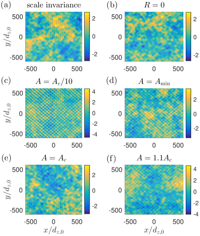
Figure 3: (a) Coordinate space representation of the (real) field $\delta\tilde{\phi}(\mathbf{x},\tau)$, in units of $\sqrt{\hbar HV/\pi mc_{0}^{2}d_{z,0}^{2}}$ after the completion of the freezing process, where the 2D volume of the system $V=(2\kappa_{0}d_{z,0})^{2}$, with initial aspect ratio $\kappa_{0}$, and the wavevector separation is chosen to be $\Delta k=2\pi/2\kappa_{0}d_{z,0}$. The statistical self-similarity reveals itself by the same degree of “wrinkliness” on each scale. (b) The field obtained from numerical implementation of the full Bogoliubov equations ($A=A_{c}/10$, $R=0$). Plots (c) through (f) are for increasing $A$ and dominating DDI ($R=\sqrt{\pi/2}$).

The solution (12) represents phonons residing in the low-momentum corner of the Bogoliubov dispersion relation [see Fig. 1 (a)]. In order to incorporate trans-Planckian dispersion and to describe its influence on the small $k$ regime, we consider the more general Bogoliubov equations (7). We start by rewriting (7) in terms of $s$

$$\delta\tilde{\phi}^{\prime\prime}_{k}-\frac{G(\zeta)^{2}-\frac{(a\zeta)^{4}}{4A}}{G(\zeta)^{2}+\frac{(a\zeta)^{4}}{4A}}\frac{1}{s}\delta\tilde{\phi}^{\prime}_{k}+\left[\frac{(a\zeta)^{4}}{4A}+G(\zeta)^{2}\right]\delta\tilde{\phi}_{k}=0,$$ (14)

where prime denotes $s$ derivatives, and $G(\zeta)^{2}:={V_{\mathrm{int},0}^{2\mathrm{D}}}(\zeta)/{g_{0}^{\mathrm{eff}}}$. Taking into account (8) and (6), the linear dispersion occurs for wavenumbers satisfying

$$\frac{(a\zeta)^{2}}{4A}\ll G(\zeta)^{2}\quad\mbox{($\Rightarrow$ analogue Planck scale $\zeta_{\rm PL}$}).$$ (15)

For small $\zeta$, $G(\zeta)^{2}\rightarrow 1$, and Eq. (15) defines $\zeta_{\rm PL}$. Experiments will generally probe sub-Planckian $\zeta$ that satisfy (15). Therefore, we consider (14) given (15) is fulfilled,

$$\delta\tilde{\phi}^{\prime\prime}_{k}-\frac{1}{s}\delta\tilde{\phi}^{\prime}_{k}+G(\zeta)^{2}\delta\tilde{\phi}_{k}=0.$$ (16)

From (11), we have $4H^{2}=\omega^{2}(0)$ (for $\omega_{0}^{2}\ll 4H^{2}$). Setting $\kappa_{0}=50$, $\omega_{z,0}=2\pi\times 2921$Hz results in $H=183.5\,$sec^-1. Given $n_{f}$ e-folds of the scale factor $a(t_{f})=\exp[n_{f}]$, the final lab time is $t_{f}=(\exp[4n_{f}]-1)/4H$. For 2.5 $e$-folds, then, $t_{f}\sim 30$ sec in lab time (for $w_{z,0}=2\pi\times 3952$ Hz, $H=248.3$ sec^-1, and 2 e-folds, $t_{f}\sim 3$ sec). We introduce a momentum cutoff $\zeta_{c}\lesssim 0.1$ which meets (15) at late times. Fig. 4 displays $\Delta^{2}(k)$, and clearly shows the deviations from SIPS, occurring for strongly dipolar interactions. When $R=0$, Eq. (16) becomes identical to the wave equation in analogue curved spacetime (9), and SIPS for long wavelengths obtains, cf. Ref. Uhlmann et al. (2005) and Fig. 4. For high momenta, there is a slight upturn in the spectrum line. As we increase the number of $e$-folds, this deviation converges to zero; for small wavelengths, it takes longer time to exit the Hubble horizon, and settling down requires longer. Using the power spectrum $\Delta^{2}(k)$, one again constructs Gaussian random fields, and the coordinate-space realization of Fig. 3  (b)–(f) is obtained, demonstrating the violation of SIPS for increasing DDI by introducing short-range correlations.

Whether SIPS is robust to trans-Planckian physics was studied in Niemeyer and Parentani (2001) (also cf. Starobinsky (2001)), where scale separation and adiabaticity in conformal time were established as sufficient conditions for SIPS. Scale separation reads ${H}/{c_{0}}\ll k_{\mathrm{Pl}}(\eta_{k})/a(\eta_{k})$, while adiabaticity holds when $\left|{c_{0}\partial_{\eta}\omega_{\eta}}/{\omega_{\eta}^{2}}\right|\ll 1\,\,\forall\,\,\eta_{i}<\eta<\eta_{f},$ where $\omega_{\eta}(\eta)$ is an effective comoving frame mode frequency Niemeyer and Parentani (2001); sup . Furthermore, $\eta_{f}$ is the ‘nonadiabatic time’ lying between $\eta_{i}$, the onset of inflation, and $\eta_{k}$, the horizon crossing, which satisfies ${H}/{c_{0}}\ll{k}/{a(\eta_{f})}\ll{k_{\mathrm{Pl}}(\eta_{k})}/{a(\eta_{k})}.$ Roughly speaking, $\eta_{f}$ is the moment when the mode stops to behave WKB-like. For de Sitter spacetime, $a=-c_{0}/H\eta$, scale separation holds when $k\ll k_{\mathrm{Pl}}(\eta_{k})$. A given $k$ thus must lie in the linear dispersion regime at horizon crossing $k\eta_{k}=-1$, which is is equivalent to imposing (15) at this point. Therefore, in our numerical implementation of the Bogoliubov equations which employs (15), scale separation is satisfied automatically. According to Niemeyer and Parentani (2001), scale separation usually implies adiabaticity, resulting in the robustness of the predictions of the inflationary scenario. However, when the spectrum has (even if only initially) a deep minimum, as here, adiabaticity can be violated even when scale separation holds, and SIPS breaks down.

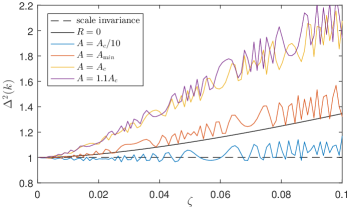
Figure 4: $\Delta^{2}(k)=k^{2}P(k)$ as a function of in-plane momentum $\zeta$, for 2.5 e-folds. Black dashed line represent SIPS. The black solid line corresponds to contact interaction, $R=0$ ($A=A_{c}/10$). The other lines correspond to DDI domination ($R=\sqrt{\pi/2}$), with values of $A$ as specified in the inset. In the long-wavelength limit, they all converge to SIPS. The slope of the $R=0$ curve decreases for increasing number of e-folds, asymptotically yieldding SIPS for pure contact interactions.

In conclusion, we have found that for contact interactions, $R=0$, SIPS is retained (in the limit of many e-folds), while there appear strong deviations from scale invariance in the presence of strong DDI (Fig. 4) due to an initially present roton minimum. Importantly, the influence of the trans-Planckian nonlinear dispersion is manifest even far from criticality at $A_{c}$. When a negative slope in the excitation spectrum occurs ($A>A_{\mathrm{min}}$ in  Fig.1), the power spectrum shows a general tendency of increase at high momenta. On the other hand, for monotonously increasing spectrum, when $A\leq A_{\mathrm{min}}$, the power spectrum oscillates around the SIPS prediction.

We stress that the presence of a minimum in the spectrum does not necessarily imply violations of scale invariance. It is possible to construct an analytic solution to the full Bogoliubov equations for a spectrum with minimum, which displays SIPS sup . The proposed experiment (or variants thereof, possibly with other engineered interaction potentials) can thus potentially lead to conclusions about the trans-Planckian physics of quantum fields in early cosmological stages. We also note in this regard that SIPS is a kinematical effect for quantum fields in de Sitter spacetime, in analogy to Hawking radiation from black holes Visser (1998b), and therefore, like the latter, does not require the Einstein equations to hold.

Going beyond mean-field theory, future perspectives include to study the influence of strong quantum fluctuations of high density electrically dipolar gases Baranov et al. (2012), prevailing in an early, possibly pre-metric stage, onto the analogue cosmological evolution in the inflationary scenario.

This research was supported by the NRF Korea, Grant No. 2014R1A2A2A01006535.

I Supplemental Material

I.1 Action of the system

I.1.1 Dimensional reduction

In the limit of zero-point energy of the axial harmonic oscillator greatly exceeding the chemical potential, and for large aspect ratio, the longitudinal and transversal degrees of freedom decouple and we can factorize the order parameter $\Psi(\mathbf{R},t)$ as follows

$$\Psi(\mathbf{R},t)=\Psi_{r}(\mathbf{r},t)\Phi_{z}(z)e^{-i\omega_{z}t/2}.$$ (S1)

Here $\Phi_{z}(z)$ describes the zero point oscillations in a harmonic oscillator potential, and is given by

$$\Phi_{z}(z)=\frac{1}{(\pi d_{z}^{2})^{1/4}}\exp\Bigl{[}-\frac{z^{2}}{2d_{z}^{2}}\Bigr{]},$$

where $d_{z}=\sqrt{\hbar/m\omega_{z}}$ is the oscillator length. Improved estimates for $d_{z}$ can be found by treating $d_{z}$ as a parameter minimizing the Gross-Pitaevskiǐ  ground-state energy Fischer (2006); Giovanazzi and O’Dell (2004).

Substituting (S1) into the action (1), and integrating out the $z$ dependence, we obtain the reduced Lagrangian for the horizontal in-plane mode:

$$\mathcal{L}_{r} =\frac{i\hbar}{2}(\Psi_{r}^{*}\partial_{t}{\Psi}_{r}-\partial_{t}{\Psi}_{r}^{*}\Psi_{r})-\frac{\hbar^{2}}{2m}|\nabla_{r}\Psi_{r}|^{2}-\frac{m}{2}\omega^{2}r^{2}|\Psi_{r}|^{2}-\frac{g_{c}^{2\mathrm{D}}}{2}|\Psi_{r}|^{4}-\frac{1}{2}|\Psi_{r}|^{2}\int d^{2}\mathbf{r}^{\prime}\,V_{dd}^{2\mathrm{D}}(\mathbf{r}-\mathbf{r}^{\prime})|\Psi_{r}(\mathbf{r}^{\prime})|^{2},$$

where $\nabla_{r}=(\partial_{x},\partial_{y})$. The contact coupling is reduced to $g_{c}^{2\mathrm{D}}=g_{c}/\sqrt{2\pi}d_{z}$, and the reduced lower-dimensional DDI is given by ($\rho_{z}=|\Phi_{z}|^{2}$)

$$V_{dd}^{2\mathrm{D}}(\mathbf{r}-\mathbf{r}^{\prime})=\int dzdz^{\prime}\,V_{dd}(\mathbf{R}-\mathbf{R}^{\prime})\rho_{z}(z)\rho_{z}(z^{\prime}).$$ (S2)

We assume the dipoles to be polarized along $z$-direction by an external field, so that their interaction is

$$V_{dd}(\mathbf{R},t)=\frac{3g_{d}}{4\pi}\frac{1-3z^{2}/|\mathbf{R}|^{2}}{|\mathbf{R}|^{3}},$$ (S3)

where $g_{d}=\mu d_{m}^{2}/3$ for magnetic and $g_{d}=d_{e}^{2}/3\epsilon$ for electric dipoles.

The nature of this interaction can be seen clearly by looking at its Fourier space representation. The Fourier transform of the DDI (S3) takes the well-known form

$${V}_{dd}(\mathbf{Q})=g_{d}\Bigl{(}\frac{3q_{z}^{2}}{Q^{2}}-1\Bigr{)},$$

where $\mathbf{Q}=(\mathbf{q},q_{z})$. Here and below, we will use asymmetric Fourier convention in which the inverse transform incorporates the whole prefactor. The Fourier transform of the density profile in $z$-direction $\rho_{z}$, for homogeneous density in the 2D plane, is given by ${\rho}_{z}(\mathbf{Q})=V\delta^{(2)}_{\mathbf{q},0}\exp[-q_{z}^{2}d_{z}^{2}/4]$, where $V$ is the area of the plane. Substituting the inverse Fourier transforms of these expressions into (S2), we obtain Fischer (2006)

$$V_{dd}^{2\mathrm{D}}(\mathbf{r}-\mathbf{r}^{\prime})=\frac{g_{d}}{V}\sum_{\mathbf{q}}e^{i\mathbf{q}\cdot(\mathbf{r}-\mathbf{r}^{\prime})}\biggl{\{}\frac{2}{\sqrt{2\pi}d_{z}}-\frac{3q}{2}w\biggl{[}\frac{qd_{z}}{\sqrt{2}}\biggr{]}\biggr{\}}.$$ (S4)

Here we made use of an integral representation of the error function Abramowitz and Stegun (1970)

$$w(z):=e^{z^{2}}\mathrm{erfc}(z)=\frac{2z}{\pi}\int_{0}^{\infty}\frac{e^{-t^{2}}}{z^{2}+t^{2}}dt\quad(z>0),$$ (S5)

where the complementary error function is defined as $\mathrm{erfc}(z)=1-\mathrm{erf}(z)=1-(2/\sqrt{\pi})\int_{0}^{z}\exp(-t^{2})dt$.

From (S4), we see that the DDI contributes to the delta-function-like interaction as well as to the nonlocal one. It is convenient to decompose the total (contact and dipolar) interaction into a sum of effective contact interaction and nonlocal interaction:

$$g^{\mathrm{eff}}\delta^{(2)}(\mathbf{r}-\mathbf{r}^{\prime})+U^{2\mathrm{D}}(\mathbf{r}-\mathbf{r}^{\prime}),$$ (S6)

where the effective contact coupling strength is defined by

$$g^{\mathrm{eff}}:=g_{c}^{2\mathrm{D}}+\frac{2g_{d}}{\sqrt{2\pi}d_{z}}=\frac{1}{\sqrt{2\pi}d_{z}}(g_{c}+2g_{d}),$$

and the nonlocal interaction is written as

$$U^{2\mathrm{D}}(\mathbf{r}-\mathbf{r}^{\prime})=-\frac{3}{2}\frac{g_{d}}{V}\sum_{\mathbf{q}}e^{i\mathbf{q}\cdot(\mathbf{r}-\mathbf{r}^{\prime})}qw\biggl{[}\frac{qd_{z}}{\sqrt{2}}\biggr{]}.$$

I.1.2 Scaling transformation

Having performed dimensional reduction, we consider the action

$$\mathcal{L} =\frac{i\hbar}{2}(\Psi^{*}\dot{\Psi}-\dot{\Psi}^{*}\Psi)-\frac{\hbar^{2}}{2m}|\nabla\Psi|^{2}-\frac{m}{2}\omega^{2}r^{2}|\Psi|^{2}-\frac{g^{\mathrm{eff}}}{2}|\Psi|^{4}-\frac{1}{2}|\Psi|^{2}\int d^{2}\mathbf{r}^{\prime}\,U^{2\mathrm{D}}(\mathbf{r}-\mathbf{r}^{\prime})|\Psi(\mathbf{r}^{\prime})|^{2},$$ (S7)

where we dropped subscripts for conciseness. We can prescribe an external time dependences not only with a temporal profile of the trap frequencies but also to $g_{c}=4\pi\hbar^{2}a_{s}/m$ and $g_{d}$ by changing the $s$-wave scattering length $a_{s}$ via Feshbach resonances Courteille et al. (1998); Inouye et al. (1998) and using a rotating polarizing field to change $g_{d}$ Giovanazzi et al. (2002), respectively. As a result, the gas cloud will adapt to these changes and will either expand or contract.

A part of this background motion can be accounted for by transforming to a new coordinate system

$$\mathbf{x}:=\frac{\mathbf{r}}{b(t)},\qquad\tau:=\int_{0}^{t}\frac{1}{b^{2}(t^{\prime})}dt^{\prime},$$ (S8)

with a scale factor $b(t)$. Following Kagan et al. (1996), define $\psi(\mathbf{x},\tau)$ by

$$\Psi(\mathbf{r},t):=e^{i\Phi}\frac{\psi(\mathbf{x},\tau)}{b},$$ (S9)

where $\Phi(\mathbf{x},t)=\frac{1}{2}\frac{m}{\hbar}r^{2}\frac{\partial_{t}{b}}{b}$ is chosen so as to describe the bulk velocity $\mathbf{v}=\dot{\mathbf{x}}=-\frac{1}{b}\frac{\hbar}{m}\nabla\Phi$, while the phase of $\psi$ will represent the residual velocity potential, which can be regarded as small. Insertion of this ansatz into the action (S7) yields

$$\mathcal{L} =\frac{i\hbar}{2}(\psi^{*}\partial_{\tau}\psi-\partial_{\tau}\psi^{*}\psi)-\frac{\hbar^{2}}{2m}|\nabla_{x}\psi|^{2}-\frac{m}{2}x^{2}\left(\frac{d^{2}b}{dt^{2}}{b^{3}}+\omega^{2}b^{4}\right)|\psi|^{2}-\frac{g^{\mathrm{eff}}}{2}|\psi|^{4}$$

$$\quad-\frac{g_{d}}{2g_{d,0}b}\int d^{2}\mathbf{x}^{\prime}\,U^{2\mathrm{D}}_{0}(\mathbf{x}-\mathbf{x}^{\prime})|\psi(\mathbf{x})|^{2}|\psi(\mathbf{x}^{\prime})|^{2}.$$ (S10)

Note that the measure $dtd^{2}\mathbf{r}$ gives an additional factor of $b^{4}$ by the relation $dtd^{2}\mathbf{r}=b^{4}d\tau d^{2}\mathbf{x}$. The scaled nonlocal interaction is written as

$$U^{2\mathrm{D}}_{0}(\mathbf{x}-\mathbf{x}^{\prime})=-\frac{3}{2}\frac{g_{d,0}}{V}\sum_{\mathbf{k}}e^{i\mathbf{k}\cdot(\mathbf{x}-\mathbf{x}^{\prime})}kw\bigg{[}\frac{kd_{z,0}}{\sqrt{2}}\biggr{]},$$

where $g_{d,0}$ and $d_{z,0}$ are initial values. In order to obtain this expression, we have assumed a scaling condition

$$d_{z}(t)=d_{z,0}b(t)\quad\text{ or }\quad\omega_{z}(t)=\frac{\omega_{z,0}}{b^{2}(t)}.$$ (S11)

We can combine the remaining time dependences into a single factor $f(t)$ by imposing (4). Here $g_{c,0}$ is the initial value and $\omega_{0}$ will be fixed when a specific solution to the scaling equation is chosen. Examples of analytic solutions to the scaling equation (4) are presented in (S25) and (11). Under these scaling conditions, the action (S10) becomes

$$\mathcal{L} =\frac{i\hbar}{2}(\psi^{*}\partial_{\tau}\psi-\psi\partial_{\tau}\psi^{*})-\frac{\hbar^{2}}{2m}{|\nabla_{x}\psi|^{2}}-f^{2}\biggl{[}\frac{m}{2}\omega_{0}^{2}x^{2}|\psi|^{2}+\frac{g^{\mathrm{eff}}_{0}}{2}|\psi|^{4}+\frac{1}{2}\int d^{2}\mathbf{x}^{\prime}\,U^{2\mathrm{D}}_{0}(\mathbf{x}-\mathbf{x}^{\prime})|\psi(\mathbf{x})|^{2}|\psi(\mathbf{x}^{\prime})|^{2}\biggr{]}.$$ (S12)

I.1.3 Hydrodynamic variables and a background solution

In terms of the Madelung representation for the scaled order parameter, $\psi=\sqrt{\rho}e^{i\phi}$, the equation of motion (3) can be recast as

$$\partial_{\tau}\rho =-\frac{\hbar}{m}(\nabla_{x}\phi\cdot\nabla_{x}\rho+\rho\nabla_{x}^{2}\phi),$$

$$-\hbar\partial_{\tau}\phi =-\frac{\hbar^{2}}{2m\sqrt{\rho}}\nabla_{x}^{2}\sqrt{\rho}+\frac{\hbar^{2}}{2m}(\nabla_{x}\phi)^{2}+f^{2}\frac{m}{2}\omega_{0}^{2}x^{2}+f^{2}\int d^{2}\mathbf{x}^{\prime}\,V^{2\mathrm{D}}_{\mathrm{int},0}(\mathbf{x}-\mathbf{x}^{\prime})\rho(\mathbf{x}^{\prime}),$$ (S13)

where $V^{2\mathrm{D}}_{\mathrm{int},0}(\mathbf{x}-\mathbf{x}^{\prime})=g_{0}^{\mathrm{eff}}\delta^{(2)}(\mathbf{x}-\mathbf{x}^{\prime})+U_{0}^{2\mathrm{D}}(\mathbf{x}-\mathbf{x}^{\prime})$. If we linearize the fields around stationary background solutions, $\rho=\rho_{0}+\delta\rho,\,\phi=\phi_{0}+\delta\phi$, the zeroth order equations are the same as (S13) with subscripts $0$ attached to the fields, and the first order equations are the Bogoliubov equations (5).

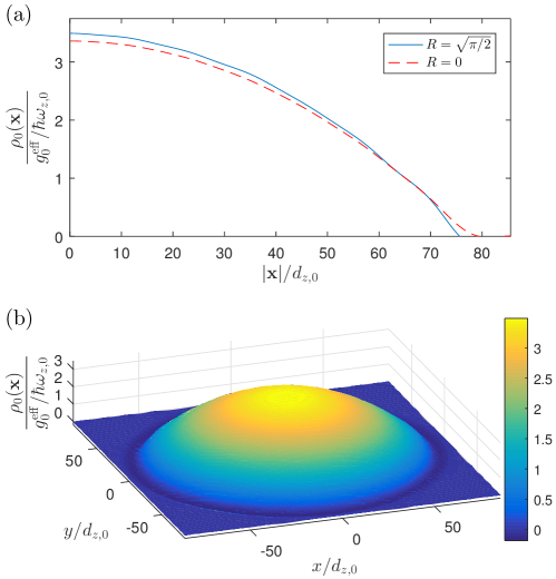
Figure S1: The density profile of the gas in units of $g^{\mathrm{eff}}_{0}/\hbar\omega_{z,0}$ as a function of radial distance in units of $d_{z,0}$. In (a), blue solid and red dashed line corresponds to DDI-dominant and contact-dominant cases, repectively. We also present a visualization of the gas in (b), using parameters appropriate for erbium atoms Aikawa et al. (2012). Namely, particle number $N=9.5\times 10^{4}$, magnetic moment $d_{m}=7\,\mu_{B}$, boson mass $m=168\,\mathrm{u}$, aspect ratio $\kappa_{0}=30$, and transverse trapping frequency $\omega_{z,0}=2\pi\times 5435$ Hz.

We solve the zeroth order equations assuming vanishingly small residual comoving frame velocity ($\mathbf{v}_{\rm com}:=\frac{\hbar}{m}\nabla_{x}\phi_{0}=0$) by the ansatz $\psi_{0}(\mathbf{x},\tau)=\sqrt{\rho_{0}(\mathbf{x})}e^{i\phi_{0}(\tau)}$ Uhlmann et al. (2005), and neglect the kinetic energy term, which is equivalent to neglecting terms proportional to $\nabla_{x}^{2}\sqrt{\rho_{0}}$. Then we obtain a spatially constant phase function

$$\phi_{0}(\tau)=-\frac{\mu_{0}}{\hbar}\int_{0}^{\tau}d\tau^{\prime}\,f^{2}(\tau^{\prime}),$$ (S14)

where $\mu_{0}$ is initial chemical potential, and an integral equation for time independent density profile

$$\int d^{2}\mathbf{x}^{\prime}\,V^{2\mathrm{D}}_{\mathrm{int},0}(\mathbf{x}-\mathbf{x}^{\prime})\rho_{0}(\mathbf{x}^{\prime})=\mu_{0}-\frac{m}{2}\omega_{0}^{2}x^{2},$$ (S15)

which can be solved numerically. Because of the partially attractive nature of DDI, the profile shows enhanced concentration at the center compared to the pure contact case, cf. Fig. S1. Also, the anisotropy of the interaction results in the appearance of small wiggles in the density profile Parker and O’Dell (2008); Lu et al. (2010).

I.2 Gravitational analogy and an analytical solution

I.2.1 Effective geometry

Rewriting the equation (9) in real space, the resulting equation is equivalent to the phases only Lagrangian

$$\overline{\mathcal{L}^{(2)}}=\frac{\hbar^{2}/2}{f^{2}g_{0}^{\mathrm{eff}}}(D\delta\phi)^{2}-\frac{\hbar^{2}\rho_{0}}{2m}(\nabla_{x}\delta\phi)^{2},$$ (S16)

where $D=\partial_{\tau}+\mathbf{v}_{\rm com}\cdot\nabla_{x}$ is the comoving derivative.

With the metric tensor (10), the Lagrangian becomes that of a minimally coupled free scalar field in a curved spacetime

$$\overline{\mathcal{L}^{(2)}}=\frac{mc_{0}^{2}}{2}\sqrt{|g|}g^{\mu\nu}\partial_{\mu}\delta\phi\partial_{\nu}\delta\phi,$$ (S17)

where repeated indices imply summation over $\mu=0,\,1,\,2$ and $x^{0}=c_{0}\tau$.

For the background solutions (S14) and (S15), $\mathbf{v}_{\rm com}=\frac{\hbar}{m}\nabla_{x}\phi_{0}=\mathbf{0}$ and $\rho_{0}$ is time independent. In this case the line element (10) becomes

$$ds^{2}=\Omega^{-2}\bigl{(}c_{0}^{2}d\tau^{2}-a^{2}d\mathbf{x}^{2}\bigr{)},\quad a=\frac{1}{f},$$ (S18)

where the conformal factor

$$\Omega=\frac{c_{0}^{2}m^{2}}{\hbar^{2}\rho_{0}}$$ (S19)

is dimensionless. Herein, we assume that the density $\rho_{0}$ is essentially homogeneous near the center of cloud. This implies that $\omega_{0}$, the trapping frequency in the scaled coordinate system, is negligible compared to the time scale of the effective spacetime (that is the Hubble constant $H$, cf. (11)). Then $\Omega$ becomes just a constant, and the action (S17) is invariant under the conformal transformation

$$\tilde{g}_{\mu\nu}=\Omega^{2}g_{\mu\nu}\quad\text{ and }\quad\delta\tilde{\phi}=\Omega^{-1/2}\delta\phi,$$ (S20)

and the resulting metric $\tilde{g}_{\mu\nu}$ assumes the form of FRW universe

$$ds^{2}=c_{0}^{2}d\tau^{2}-a^{2}d\mathbf{x}^{2}=\tilde{g}_{\mu\nu}dx^{\mu}dx^{\nu},$$ (S21)

where $\tilde{g}_{\mu\nu}=\mathrm{diag}(1,\,-a^{2},\,-a^{2})$. Now we can apply standard techniques of quantum field theory in a FRW universe to obtain independent solutions for $\delta\tilde{\phi}$. Then the independent solutions for original field $\delta\phi$ will be obtained by $\delta\phi=\Omega^{1/2}\delta\tilde{\phi}$. In this effective spacetime, the Klein-Gordon (KG) equation for massless, minimally coupled free scalar field,

$$\Box\delta\tilde{\phi}=(1/\sqrt{|\tilde{g}|})\partial_{\mu}(\sqrt{|\tilde{g}|}\tilde{g}^{\mu\nu}\partial_{\nu}\delta\tilde{\phi})=0,$$ (S22)

takes the form of (9).

Here, for ease of connecting the current discussion to a standard cosmological context, we introduce the conformal time

$$\eta:=\int_{\infty}^{\tau}\frac{c_{0}}{a(\tau^{\prime})}\,d\tau^{\prime},$$ (S23)

which ranges from $-\infty\;(\tau\to-\infty)$ to $0\;(\tau\to\infty)$. Then the metric (S18) takes the conformally flat form $ds^{2}=a^{2}[d\eta^{2}-d\mathbf{x}^{2}]$, and the equation (9) can be recasted in terms of an auxiliary field $\chi_{k}:=\sqrt{a}\delta\tilde{\phi}_{k}$ by

$$\partial^{2}_{\eta}\chi_{k}+\left[k^{2}-\frac{\partial^{2}_{\eta}a}{2a}+\frac{(\partial_{\eta}a)^{2}}{4a^{2}}\right]\chi_{k}=0\quad\Leftrightarrow\quad\partial^{2}_{\eta}\chi_{k}+\omega^{2}_{\eta}(\eta)\chi_{k}=0.$$ (S24)

Comparing this equation with Eq. (1) in Niemeyer and Parentani (2001), one identifies $\omega_{\eta}$ as an effective comoving frame mode frequency. The choice of auxiliary field $\chi_{k}$ is motivated by removing the first derivative term in (9).

I.2.2 Mode functions in $2+1$-dimensional de Sitter spacetime

We consider de Sitter spacetime by setting $a(\tau)=1/f(\tau)=e^{H\tau}$. There are several simple analytic solutions to the scaling equation (4) for the realization of analogue de Sitter spacetime. For example one can consider $b:=1\,\forall\,t$, so that scaling time equals lab time, $\tau=t$, and obtain the scale factor evolution

$$a^{-2}(t)=e^{-2Ht}=\frac{\omega^{2}}{\omega_{0}^{2}}=\frac{g_{c}}{g_{c,0}}=\frac{g_{d}}{g_{d,0}}.$$ (S25)

While this expansion has the advantage of scaling and lab time being identical, $\tau:=t$, it is experimentally challenging to realize because of the (simultaneously) exponentially in time varying coupling constants. Another analytic solution, which is found by imposing $g_{d}:=g_{d,0}$, gives (11). This solution implies $g_{c}$ as well as $g_{d}$ to be constant. Our numerical analysis is based on this solution. Note that we assume $\omega_{0}$ to be negligible compared to $H$ in the quasihomogeneous limit.

A simple parameter can help us understand the underlying physical process and characterize appropriate asymptotic regimes. Define

$$s:=\frac{c_{0}/H}{a/k}=\frac{c_{0}k}{Ha},$$ (S26)

which is the ratio of Hubble radius to the physical wavelength of a chosen mode. The parameter $s$ starts from infinity and finally approaches 0. Note that, in the de Sitter analogue $a=e^{H\tau}$, the conformal time becomes $\eta=-c_{0}/Ha$, and the parameter $s$ can be written employing conformal time simply as $s=-k\eta$. One can see that the horizon crossing time $\eta_{k}$ of a chosen wavenumber $k$ is determined by $s=1$ or $k=a(\eta_{k})H/c_{0}$. In the de Sitter analogue, $a=-c_{0}/H\eta$, the horizon crossing time is the moment when

$$k\eta_{k}=-1.$$ (S27)

The equation (9) can now be written as

$$\delta\tilde{\phi}_{k}^{\prime\prime}-\frac{1}{s}\delta\tilde{\phi}_{k}^{\prime}+\delta\tilde{\phi}_{k}=0,$$ (S28)

where prime denotes taking derivative with respect to $s$.

Large $s$ implies that the mode is well inside the Hubble radius and does not feel the curvature of the analogue spacetime. When $a$ is small, i.e., before the inflation, the condition $s\gg 1$ is satisfied for wide range of $k$ and so all the relevant modes are well inside the Hubble radius. At this epoch, the second term in (9) can be neglected and we get the WKB solution for time varying frequency $\omega_{k}=c_{0}k/a$:

$$\delta\tilde{\phi}_{k}\longrightarrow\sqrt{\frac{\hbar V}{2ma^{2}Hs}}\exp(is)=\sqrt{\frac{\hbar V}{2ma^{2}\omega_{k}}}\exp\left(-i\int_{\infty}^{\tau}\omega_{k}(\tau^{\prime})d\tau^{\prime}\right),$$ (S29)

where coefficients are chosen by imposing the normalization condition $\bigl{(}\delta\tilde{\phi}_{k}e^{i\mathbf{k}\cdot\mathbf{x}}/V,\,\delta\tilde{\phi}_{k}e^{i\mathbf{k}^{\prime}\cdot\mathbf{x}}/V\bigr{)}_{\mathrm{KG}}=\delta^{(2)}_{\mathbf{k},\mathbf{k}^{\prime}}$ and the conserved Klein-Gordon (KG) inner product is defined by Kurita et al. (2009); Barceló et al. (2010)

$$(f,g)_{\mathrm{KG}} =i\frac{mc_{0}}{\hbar}\int d^{2}\mathbf{x}\,\sqrt{|\gamma|}f^{*}(\mathbf{x},\tau)\overleftrightarrow{\partial_{n}}g(\mathbf{x},\tau)$$ (S30)

$$=i\frac{mc_{0}^{2}}{\hbar}\int d^{2}\mathbf{x}\,\frac{a^{2}}{c_{0}^{2}}f^{*}(\mathbf{x},\tau)\overleftrightarrow{\partial_{\tau}}g(\mathbf{x},\tau).$$

Here, $\gamma$ is the determinant of the metric in the spatial slice $\tau=\mathrm{const.}$, $n^{\mu}$ is its normal, and $\partial_{n}=n^{\mu}\partial_{\mu}$.

We note that, with this choice of coefficients, the canonical commutation relation, $\bigl{[}\delta\hat{\tilde{\phi}}(\mathbf{x},\tau),\,\delta\hat{\tilde{\pi}}(\mathbf{y},\tau)\bigr{]}=i\hbar\delta^{(2)}(\mathbf{x}-\mathbf{y})$, with conjugate momentum $\delta\tilde{\pi}=\partial\overline{\mathcal{L}^{(2)}}/\partial(\partial_{\tau}\delta\tilde{\phi})=ma^{2}\partial_{\tau}\delta\tilde{\phi}$ holds, and the proper (diagonalized) expression for the energy $\overline{H^{(2)}}=\sum_{\mathbf{k}}\hbar\omega_{k}(\hat{a}_{\mathbf{k}}^{\dagger}\hat{a}_{\mathbf{k}}+1/2)$ can be obtained.

It is possible to obtain an analytic solution to (S28) over the whole range of time. Following Mukhanov and Winitzki (2007); Parker and Toms (2009), we define a function $F$ by

$$F(s)=\frac{1}{s}\delta\tilde{\phi}_{k}.$$

Then (S28) becomes the Bessel equation of order 1:

$$s^{2}F^{\prime\prime}+sF^{\prime}+(s^{2}-1)F=0,$$

whose general solution can be written as a linear combination of Bessel functions $J_{1}$ and $Y_{1}$ Abramowitz and Stegun (1970). Thus we obtain

$$\delta\tilde{\phi}_{k}(s)=s\Bigl{[}A(k)J_{1}(s)+B(k)Y_{1}(s)\Bigr{]}.$$ (S31)

We can determine the coefficients $A(k)$ and $B(k)$ by matching this solution with the WKB solution (S29) in the $s\to\infty$ limit. Recalling the asymptotic behavior of Bessel functions Abramowitz and Stegun (1970), we see that, for fixed $\eta$,

$$B(k)\to iA(k),\quad A(k)\to\sqrt{\frac{\pi\hbar VH}{4mc_{0}^{2}k^{2}}}\quad\text{ as }k\to\infty,$$

must be fulfilled in order to match the WKB solution (S29) up to a constant phase.

We invoke de Sitter invariance to determine $A(k)$ and $B(k)$ for all $k$. We observe that the metric (S21) with $a(\tau)=e^{H\tau}$ is invariant under the transformation

$$\tau \to\tau^{\prime}=\tau+\tau_{1},$$

$$\mathbf{x} \to\mathbf{x}^{\prime}=e^{-H\tau_{1}}\mathbf{x},$$

where $\tau_{1}$ is arbitrary. If we define $\mathbf{k}^{\prime}:=\mathbf{k}e^{H\tau_{1}}$, we have $\mathbf{k}^{\prime}/a(\tau^{\prime})=\mathbf{k}/a(\tau)$ and $\mathbf{k}\cdot\mathbf{x}=\mathbf{k}^{\prime}\cdot\mathbf{x}^{\prime}$. Thus we obtain

$$\delta\tilde{\phi}_{k^{\prime}}(s)=s\Bigl{[}A(k^{\prime})J_{1}(s)+B(k^{\prime})Y_{1}(s)\Bigr{]},$$

since $s$ is unchanged when $\tau\to\tau^{\prime}$ and $k\to k^{\prime}$. From the invariance of the metric, it follows that $\delta\tilde{\phi}_{k^{\prime}}(s)e^{i\mathbf{k}^{\prime}\cdot\mathbf{x}^{\prime}}/V^{\prime}=\delta\tilde{\phi}_{k}(s)e^{i\mathbf{k}\cdot\mathbf{x}}/V$ and so

$$\frac{A(k)}{V}=\frac{A(k^{\prime})}{V^{\prime}}$$

for any $k$ and any $\tau_{1}$. Taking $\tau_{1}\to\infty$, the r.h.s. converges to $(1/V)\sqrt{\pi\hbar VH/4mc_{0}^{2}k^{2}}$. Therefore we conclude that $A(k)=\sqrt{\pi\hbar VH/4mc_{0}^{2}k^{2}}$ for any $k$ and the mode function is written as in (12).

We finally obtain the mode expansion for the phase fluctuation field:

$$\delta\hat{\tilde{\phi}}(\mathbf{x},\tau)=\sum_{\mathbf{k}}\hat{\tilde{a}}_{\mathbf{k}}f^{(0)}_{\mathbf{k}}(\mathbf{x},\tau)+\hat{\tilde{a}}_{\mathbf{k}}^{\dagger}f^{(0)*}_{\mathbf{k}}(\mathbf{x},\tau),$$ (S32)

where $\hat{\tilde{a}}_{\mathbf{k}}$ and $\hat{\tilde{a}}_{\mathbf{k}}^{\dagger}$ are time independent creation/annihilation operators obeying the commutation relations $[\hat{\tilde{a}}_{\mathbf{k}},\,\hat{\tilde{a}}_{\mathbf{k}^{\prime}}^{\dagger}]=\delta^{(2)}_{\mathbf{k},\mathbf{k}^{\prime}}$. The mode function is written as

$$f^{(0)}_{\mathbf{k}}(\mathbf{x},\tau)=\frac{1}{V}h_{k}(s)e^{i\mathbf{k}\cdot\mathbf{x}}.$$

The vacuum corresponding to the basis $\hat{\tilde{a}}_{\mathbf{k}}$ is the Bunch-Davies vacuum Bunch and Davies (1978). Note that at this stage the relation between what $\hat{\tilde{a}}_{\mathbf{k}}^{\dagger}$ creates and the Bogoliubov quasiparticles is not clear. We will establish a direct connection between them below in (S60).

I.2.3 Correlation function

The correlations of a fluctuating quantum field are a measurable quantity in an experimental setup. Thus we investigate the spatially Fourier-transformed two-point correlation function, which is defined by Fischer and Schützhold (2004)

$$C_{\delta\tilde{\phi}}(\mathbf{k},\tau)=\int_{V}d^{2}\mathbf{x}\,e^{-i\mathbf{k}\cdot\mathbf{x}}\bigl{\langle}\delta\hat{\tilde{\phi}}(0,\tau)\delta\hat{\tilde{\phi}}(\mathbf{x},\tau)\bigr{\rangle}.$$

Now we insert the the mode expansion (S32). Recalling the asymptotic behavior of the Bessel functions, we have

$$h_{k}(s)\to-i\sqrt{\frac{\hbar VH}{\pi mc_{0}^{2}}}\frac{1}{k},\quad\text{ as }s\to 0,$$

and obtain

$$C_{\delta\tilde{\phi}}(\mathbf{k},\tau)=\frac{|h_{k}|^{2}}{V}\>\to\>\frac{\hbar H}{\pi mc_{0}^{2}}\frac{1}{k^{2}}.$$ (S33)

Note that the mode function and correlation function become time independent at late times. Thus the density fluctuations determined by (5) vanish at zeroth order. In order to obtain nontrivial density fluctuations, one has to take the time dependence of the phase fluctuations into account, which is beyond the zeroth-order frozen part.

I.2.4 Scale invariant power spectrum

The amplitude of quantum fluctuations is always well defined irrespective of whether the particle interpretation of a given field is available Mukhanov and Winitzki (2007). One way to characterize the typical fluctuations on scales $L$ is to calculate the variance $\delta\chi_{L}^{2}(\tau)=\langle 0|[\hat{\chi}_{L}(\tau)]^{2}|0\rangle$ of the field operator averaged over a region of size $L$:

$$\hat{\chi}_{L}(\tau):=\int d^{2}\mathbf{x}\,\delta\hat{\tilde{\phi}}(\mathbf{x},\tau)W_{L}(\mathbf{x}),$$

where $W_{L}(\mathbf{x})$ is a window function which is of order 1 for $|\mathbf{x}|\lesssim L$ and rapidly decays for $|\mathbf{x}|\gg L$. It is prototypically specified in terms of Gaussian function $W_{L}(\mathbf{x})=(1/2\pi L^{2})\exp(-|\mathbf{x}|^{2}/2L^{2})$. Given the mode expansion (S32), after straightforward algebra with an approximation to the Fourier transform of the unit ($L=1$) window function, $w(\mathbf{k})\simeq 2\pi[1-\theta(k-1)]$, one can find

$$\delta\chi_{L}^{2}(\tau)\simeq\int_{0}^{L^{-1}}\frac{dk}{k}\frac{k^{2}|h_{k}|^{2}}{V}.$$

We define the (two-dimensional version of) power spectrum $P(k)$ to be proportional to the variance per $\ln k$:

$$k^{2}P(k):=\Delta^{2}(k)=\frac{d\delta\chi_{L}^{2}}{d\ln k}=\frac{k^{2}|h_{k}|^{2}}{V},\quad k=L^{-1}.$$

Another characterization of the power spectrum is as the Fourier transform of the correlation function Peacock (1999):

$$\xi(\mathbf{x}-\mathbf{y}) =\langle 0|\delta\hat{\tilde{\phi}}(\mathbf{x},\tau)\delta\hat{\tilde{\phi}}(\mathbf{y},\tau)|0\rangle$$

$$:=\frac{1}{V}\sum_{\mathbf{k}}P(k)e^{i\mathbf{k}\cdot(\mathbf{x}-\mathbf{y})}.$$ (S34)

from which we have $P(k)=\langle\delta\hat{\tilde{\phi}}_{\mathbf{k}}\delta\hat{\tilde{\phi}}_{\mathbf{k}}^{\dagger}\rangle/V=|h_{k}|^{2}/V$, where $\delta\hat{\tilde{\phi}}_{\mathbf{k}}$ is the Fourier transform of the mode expansion (S32). Note that $P(k)$ is nothing but the correlation function obtained in (S33). At late times, $\eta\to 0$, the power spectrum $P(k)$ converges to $\hbar H/\pi mc_{0}^{2}k^{2}$ and we see that $\Delta^{2}(k)=k^{2}P(k)$ becomes independent of $k$. We thus obtain, after the freezing process, a spectrum in which $\Delta^{2}(k)$, the variance per $\ln k$ Peacock (1999), is constant. This is called a scale-invariant power spectrum (SIPS): The universe has the same degree of ‘wrinkliness’ on each resolution scale. One can also understand this concept by observing that $|\delta\tilde{\phi}_{k}|^{2}\propto\frac{1}{k^{2}}$, namely the probability amplitude of a fluctuation having wavelength $1/k$ is proportional to the volume(area) of the space that the fluctuation is filling. Thus the general shape of the fluctuation field will be independent of the resolution scale.

It is commonly argued that the prediction of scale invariance arises because de Sitter space is invariant under time translation: there is no natural origin of time under exponential expansion Peacock (1999). At a given moment of time, the only length scale in the model is the horizon size $c_{0}/H$, so it is inevitable that the fluctuations that exist on this scale are the same at all time. If one ignores their evolution while they are outside the horizon, the resulting fluctuations give us the scale-invariant or Harrison-Zel’dovich-Peebles spectrum Harrison (1970); Zel’dovich (1972); Peebles and Yu (1970).

Regarding the phase fluctuation field $\delta\hat{\tilde{\phi}}(\mathbf{x},\tau)$ as a homogeneous and isotropic Gaussian random field Mukhanov (2005), i.e. a field whose Fourier coefficients $\delta\tilde{\phi}_{\mathbf{k}}=a_{\mathbf{k}}+ib_{\mathbf{k}}$ are random variables with probability function of the form,

$$p(a_{\mathbf{k}},b_{\mathbf{k}})=\frac{1}{\pi\sigma_{k}^{2}}e^{-a_{\mathbf{k}}^{2}/\sigma_{k}^{2}}e^{-b_{\mathbf{k}}^{2}/\sigma_{k}^{2}},$$ (S35)

the correlation function can be expressed as

$$\xi(\mathbf{x}-\mathbf{y}) =\frac{1}{V^{2}}\sum_{\mathbf{k},\mathbf{k}^{\prime}}\langle\delta\tilde{\phi}_{\mathbf{k}}(\tau)\delta\tilde{\phi}_{\mathbf{k}^{\prime}}^{*}(\tau)\rangle e^{i\mathbf{k}\cdot\mathbf{x}-i\mathbf{k}^{\prime}\cdot\mathbf{y}}$$

$$=\frac{1}{V}\sum_{\mathbf{k}}\sigma_{k}^{2}e^{i\mathbf{k}\cdot(\mathbf{x}-\mathbf{y})},$$ (S36)

where one has to take into account that $a_{-\mathbf{k}}=a_{\mathbf{k}}$ and $b_{-\mathbf{k}}=-b_{\mathbf{k}}$. From (S35), one can see that $a_{\mathbf{k}}$ and $b_{\mathbf{k}}$ are real random variables with standard deviation $\sigma_{k}/\sqrt{2}$.

Comparing (S34) and (S36), we see that the variance of the random variable $\delta\tilde{\phi}_{\mathbf{k}}$ is given by $\sigma_{k}^{2}=P(k)=|h_{k}|^{2}/V\to\hbar H/\pi mc_{0}^{2}k^{2}$, from which we can obtain a real-space realization of the phase fluctuation field $\delta\hat{\tilde{\phi}}(\mathbf{x},\tau)$ as in Fig. 3 (a).

I.3 Incorporating trans-Planckian deformation

I.3.1 Generalized Klein-Gordon equation

If we rewrite (5) in real space, we obtain

$$\partial_{\tau}\delta\rho =-\frac{\hbar\rho_{0}}{m}\nabla_{x}^{2}\delta\phi,\qquad\partial_{\tau}\delta\phi =-\frac{f^{2}g_{0}^{\mathrm{eff}}}{\hbar}\mathcal{W}\delta\rho,$$ (S37)

where $\mathcal{W}$ is an integral operator defined by

$$\mathcal{W}=\int d^{2}\mathbf{x}^{\prime}\,\biggl{[}\frac{1}{V}\sum_{\mathbf{k}}\mathcal{W}_{k}e^{i\mathbf{k}\cdot(\mathbf{x}-\mathbf{x}^{\prime})}\biggr{]}\star(\mathbf{x}^{\prime}),$$ (S38)

where $\star$ stands for the argument upon which the integral operator acts. Solving the second equation in (S37) for $\delta\rho$ and substituting into the first equation, we obtain

$$\partial_{\tau}\biggl{[}\frac{a^{2}}{c_{0}^{2}}\mathcal{W}^{-1}\partial_{\tau}\delta\tilde{\phi}\biggr{]}=\nabla_{x}^{2}\delta\tilde{\phi},$$ (S39)

where $\delta\tilde{\phi}=\Omega^{-1/2}\delta\phi$ as in (S20). This is the ‘generalized’ Klein-Gordon equation with the local Lorentz invariance being broken Barceló et al. (2010).

Rewriting (S39) in momentum space, or equivalently, solving the second equation in (5) for $\delta\rho_{\mathbf{k}}$ and substituting into the first equation yields (7).

Let us again introduce an auxiliary field and discuss in the cosmological context. In order to remove the first derivative term of (7), we define $\chi_{k}:=\sqrt{a/\mathcal{W}_{k}}\delta\tilde{\phi}_{k}$, and recast (7) as

$$\partial_{\eta}^{2}\chi_{k}+\left[k^{2}\mathcal{W}_{k}-\frac{\partial^{2}_{\eta}a}{2a}\left(1-\frac{2a\partial_{\eta}\mathcal{W}_{k}}{\mathcal{W}_{k}}\right)+\frac{(\partial_{\eta}a)^{2}}{4a^{2}}\left(1-\frac{3a^{2}(\partial_{\eta}\mathcal{W}_{k})^{2}}{\mathcal{W}_{k}^{2}}+\frac{2a^{2}\partial^{2}_{\eta}\mathcal{W}_{k}}{\mathcal{W}_{k}}+\frac{4a\partial_{\eta}\mathcal{W}_{k}}{\mathcal{W}_{k}}\right)\right]\chi_{k}=0.$$ (S40)

This equation again corresponds to Eq. (1) of Niemeyer and Parentani (2001), cf. the relativistic limit above in (S24), where now the effective comoving frame mode frequency $\omega_{\eta}$ is the square root of the expression in the square brackets. It is easily observed that (S40) converges to (S24) when $\mathcal{W}_{k}=1$, i.e. in the long wavelength limit. Furthermore, (S40) becomes (S24) except a factor of $\mathcal{W}_{k}$ multiplied to $k^{2}$ when $\mathcal{W}_{k}$ is time independent (or $a$ independent). This case is discussed in the next subsection.

I.3.2 An exactly solvable case

Solving the general equation (7) requires numerical methods. We show herein that an analytic solutions under an approximation to the interaction potential and introducing a momentum cutoff is feasible.

We replace the Fourier transform of the interaction ${V}_{\mathrm{int},0}^{2\mathrm{D}}(\zeta)$ by

$$\bar{V}^{2\mathrm{D}}_{\mathrm{int},0}(\zeta)=\left\{\begin{array}[]{l@{\qquad}l}(1-\dfrac{1}{f^{2}})\dfrac{g_{0}^{\mathrm{eff}}\zeta^{2}}{4A}+{V}^{2\mathrm{D}}_{\mathrm{int},0}(\zeta)&(\zeta\leq\zeta_{c}),\\ (1-\dfrac{1}{f^{2}})\dfrac{g_{0}^{\mathrm{eff}}\zeta_{c}^{4}}{4A\zeta^{2}}+{V}^{2\mathrm{D}}_{\mathrm{int},0}(\zeta)&(\zeta>\zeta_{c}),\end{array}\right.$$ (S41)

where momentum cutoff $\zeta_{c}$ is set to include a part of trans-Planckian momenta:

$$\zeta_{c}=\zeta_{\mathrm{Pl}}\times\alpha,$$ (S42)

where $\alpha\gtrsim 1$ determines the cutoff location and gives a class of spectrum lines that yields scale invariant power spectra (cf. Eq.(S45)). Note that initially ($f=1$) the new potential $\bar{V}^{2\mathrm{D}}_{\mathrm{int},0}$ coincides with the original one ${V}^{2\mathrm{D}}_{\mathrm{int},0}$ (Fig. S2 (a)). As time passes, the excitation spectrum deviates from the true dispersion. However, the deviation is localized around the cutoff momentum $\zeta_{c}$, and the dispersion law at low energies is secured $\forall t$.

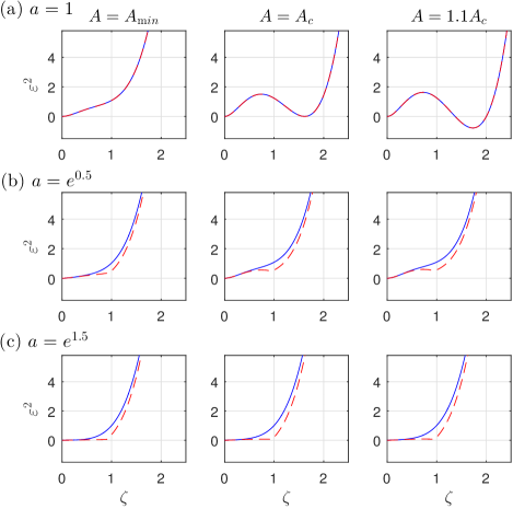
Figure S2: The squared excitation spectrum in units of $(\hbar^{2}/md_{z,0}^{2})^{2}$ at various instants of time. From left to right, the values of $A$ are $A_{\min}$, $A_{c}$ and $A_{c}\times 1.1$, repectively. $R=\sqrt{\pi/2}$ for every case. The cutoff momentum is placed at $\alpha=1.8$ (cf. (S42)). Blue lines represent the original spectrum while the red dashed lines are approximations carried out to obtain an analytic solution. Initially the two coincide and as time evolves they gradually deviate. Note that the deviation is however localized around the cutoff momentum $\zeta_{c}$.

Below the cutoff ($\zeta\leq\zeta_{c}$), the operator (6) becomes time independent

$$\mathcal{W}_{k}=\frac{\zeta^{2}}{4A}+\frac{1}{g_{0}^{\mathrm{eff}}}{V}_{\mathrm{int},0}^{2\mathrm{D}}(\zeta),$$

and equation (7) becomes

$$\delta\ddot{\tilde{\phi}}_{k}+2H\delta\dot{\tilde{\phi}}_{k}+\biggl{(}\frac{c_{0}\mathcal{K}(k)}{a}\biggr{)}^{2}\delta\tilde{\phi}_{k}=0,$$ (S43)

which is identical to (9) with $k$ being replaced with $\mathcal{K}(k)$ defined by

$$\mathcal{K}(k)^{2}:=k^{2}\mathcal{W}_{k}.$$ (S44)

We can then carry out exactly the same procedure for obtaining the mode functions (12) with $s$ being replaced with $\tilde{s}=c_{0}\mathcal{K}(k)/Ha$ and with an additional prefactor $\sqrt{\mathcal{W}_{k}}$.

With these modified mode functions, the Fourier transformed correlation function, or the power spectrum now becomes (after freezing)

$$C_{\delta\tilde{\phi}}(\mathbf{k},\tau)=\frac{|h_{k}|^{2}}{V}\;\to\;\frac{\hbar H\mathcal{W}_{k}}{\pi mc_{0}^{2}\mathcal{K}(k)^{2}},$$

and the variance per $\ln k$ becomes

$$\Delta^{2}(k)=\frac{2\hbar H\mathcal{W}_{k}}{mc_{0}^{2}}\frac{k^{2}}{\mathcal{K}(k)^{2}}=\frac{2\hbar H}{mc_{0}^{2}},$$ (S45)

which still is scale invariant. Therefore, this type of trans-Planckian deformation implied by (S41) has no effect on the power spectrum and on the matter distribution after the freezing process and SIPS is retained.

I.3.3 Numerical implementation of the full Bogoliubov equation

Let us first analyze the condition (15) in detail. Fig. S3 shows the plots of $G(\zeta)^{2}$ and $(a_{1}\zeta)^{2}/4A$ for various values of $A$ where $a_{1}$ is the final value of the scale factor. We see that, for the validity of the gravitational analogy, one can pose the later time Planck scale to be $\zeta_{\mathrm{Pl}}\lesssim 0.1$. If $\zeta<0.05$, the condition (15) is safely satisfied for all cases.

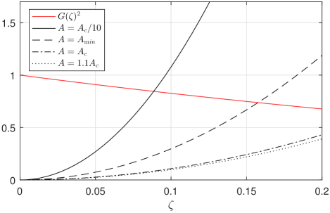
Figure S3: Plots of $G(\zeta)^{2}$ and $(a_{1}\zeta)^{2}/4A$ for various values of $A$. Here the final value of the scale factor $a_{1}$ is assumed to be $e^{5/2}$, i.e., 2.5 $e$-folds of expansion.

Before inflation, $s\to\infty$ and the second term in (16) becomes negligible. Therefore, one finds that the mode functions would converge to a WKB solution as $a\to 0$:

$$\delta\tilde{\phi}_{k}\to\sqrt{\frac{G(\zeta)\hbar VHs}{2mc_{0}^{2}k^{2}}}\exp(iG(\zeta)s),$$

where the coefficient is determined by the normalization condition $\bigl{(}\delta\tilde{\phi}_{k}e^{i\mathbf{k}\cdot\mathbf{x}}/V,\,\delta\tilde{\phi}_{k}e^{i\mathbf{k}^{\prime}\cdot\mathbf{x}}/V\bigr{)}_{\mathcal{W}-\mathrm{KG}}=\delta^{(2)}_{\mathbf{k},\mathbf{k}^{\prime}}$ where the Generalized Klein-Gordon ($\mathcal{W}$-KG) inner product is defined by the equation (S49). This solution and its derivative provides initial conditions to the second order differential equation (16). Final values (after inflation) of the mode functions $h_{k}$ then give the power spectrum via $P(k)=|h_{k}|^{2}/V$ and $\Delta^{2}(k)=k^{2}P(k)$.

I.4 Measurement

I.4.1 Bogoliubov transformation to the instantaneous Minkowski vacuum at late times

Since the de Sitter expansion is not asymptotically flat at late times, a vacuum state cannot be unambiguously defined for late times. However, the experimental verification obviously requires a choice of Fock vacuum and that choice should lead to physically reasonable results. We therefore assume, following Jain et al. (2007), that the expansion stops at some chosen moment of time $\tau_{1}$ and the gas becomes stationary, in other words, $f(\tau)=e^{-H\tau}$ for $\tau<\tau_{1}$, and $f(\tau):=f_{1}$ for $\tau\geq\tau_{1}$.

Suppose that we have obtained a complete set of “in” mode functions $f_{\mathbf{k}}^{(0)}$ for $\tau<\tau_{1}$, e.g. one obtained under (S44):

$$f_{\mathbf{k}}^{(0)}(\mathbf{x},\tau)=\frac{1}{V}h_{k}(\eta)e^{i\mathbf{k}\cdot\mathbf{x}},$$ (S46)

where the temporal part is given by

$$h_{k}(\eta)=\sqrt{\frac{\pi\hbar V\mathcal{W}_{k}}{4ma^{2}H}}\Bigl{\{}J_{1}(-\mathcal{K}(k)\eta)+iY_{1}(-\mathcal{K}(k)\eta)\Bigr{\}},$$

where $\mathcal{K}(k)$ is as defined in (S44). And suppose that a complete set of “out” mode functions $f_{\mathbf{k}}^{(1)}$ which defines the vacuum state at late times $\tau>\tau_{1}$ is given, e.g. one consists of

$$f_{\mathbf{k}}^{(1)}(\mathbf{x},\tau)=\frac{1}{V}\sqrt{\frac{\hbar V\mathcal{W}_{k}}{2ma_{1}^{2}\omega_{k1}}}e^{-i\omega_{k1}(\tau-\tau_{1})}e^{i\mathbf{k}\cdot\mathbf{x}},$$ (S47)

where $\omega_{k1}:=c_{0}\mathcal{K}(k)/a_{1}$. This is a solution to the Bogoliubov equation (S43) with $a:=a_{1}$ and $H=\frac{\dot{a}}{a}$ set equal to zero, which represents the late time behavior of the equation. The coefficients are fixed by imposing the normalization conditions ($\lambda=0,1$)

$$(f_{\mathbf{k}}^{(\lambda)},f_{\mathbf{k}^{\prime}}^{(\lambda)})_{\text{$\mathcal{W}$-$\mathrm{KG}$}}=\delta^{(2)}_{\mathbf{k},\mathbf{k}^{\prime}},\qquad(f_{\mathbf{k}}^{(\lambda)},f_{\mathbf{k}^{\prime}}^{(\lambda)*})_{\text{$\mathcal{W}$-$\mathrm{KG}$}}=0,\qquad(f_{\mathbf{k}}^{(\lambda)*},f_{\mathbf{k}^{\prime}}^{(\lambda)*})_{\text{$\mathcal{W}$-$\mathrm{KG}$}} =-\delta^{(2)}_{\mathbf{k},\mathbf{k}^{\prime}},$$ (S48)

where the generalized KG product ($\mathcal{W}$-KG inner product) is defined by Barceló et al. (2010)

$$(f,g)_{\text{$\mathcal{W}$-$\mathrm{KG}$}}=i\frac{mc_{0}^{2}}{\hbar}\int d^{2}\mathbf{x}\,\frac{a^{2}}{c_{0}^{2}}f^{*}(\mathbf{x},\tau)\overleftrightarrow{\mathcal{W}^{-1}\partial_{\tau}}g(\mathbf{x},\tau).$$ (S49)

Note that $\mathcal{W}$-KG inner product converges to the standard relativistic KG product (S30) in the limit $\mathcal{W}\to 1$.

The task at hand is to represent the “in” mode functions at $\tau>\tau_{1}$ as a linear combination of the “out” mode functions, i.e. finding the Bogoliubov coefficients $\alpha_{k},\,\beta_{k}$ in the expression

$$f_{\mathbf{k}}^{(0)}=\alpha_{k}^{*}f_{\mathbf{k}}^{(1)}+\beta_{k}^{*}f_{-\mathbf{k}}^{(1)*}$$ (S50)

for $\tau>\tau_{1}$. Then the creation/annihilation operators for “in” and “out” states will be related by

$$\hat{\tilde{a}}_{\mathbf{k}}^{(1)}=(f_{\mathbf{k}}^{(1)},\,\delta\hat{\tilde{\phi}})_{\text{$\mathcal{W}$-KG}}=\alpha_{k}^{*}\hat{\tilde{a}}_{\mathbf{k}}^{(0)}+\beta_{k}\hat{\tilde{a}}_{-\mathbf{k}}^{(0){\dagger}}.$$

Since $H={\dot{a}}/{a}$ in (S43) changes at $\tau=\tau_{1}$ in a discontinuous manner, the mode functions and their derivatives must be matched at this point:

$$f_{\mathbf{k}}^{(0)}(\tau_{1}) =\alpha_{k}^{*}f_{\mathbf{k}}^{(1)}(\tau_{1})+\beta_{k}^{*}f_{-\mathbf{k}}^{(1)*}(\tau_{1}),$$

$$\partial_{\tau}f_{\mathbf{k}}^{(0)}(\tau_{1}) =\alpha_{k}^{*}\partial_{\tau}f_{\mathbf{k}}^{(1)}(\tau_{1})+\beta_{k}^{*}\partial_{\tau}f_{-\mathbf{k}}^{(1)*}(\tau_{1}),$$

where we suppressed $\mathbf{x}$ dependence for conciseness. In the case of (S46) and (S47), solving this equation yields

$$\alpha_{k}^{*} =\sqrt{\frac{\pi\omega_{k1}}{8H}}\biggl{\{}J_{1}+Y_{1}^{\prime}+\frac{HY_{1}}{\omega_{k1}}+i\biggl{[}Y_{1}-J_{1}^{\prime}-\frac{HJ_{1}}{\omega_{k1}}\biggr{]}\biggr{\}},$$ (S51)

$$\beta_{k}^{*} =\sqrt{\frac{\pi\omega_{k1}}{8H}}\biggl{\{}J_{1}-Y_{1}^{\prime}-\frac{HY_{1}}{\omega_{k1}}+i\biggl{[}Y_{1}+J_{1}^{\prime}+\frac{HJ_{1}}{\omega_{k1}}\biggr{]}\biggr{\}},$$

where the arguments of the Bessel functions are $-\mathcal{K}(k)\eta_{1}$. Note that, if the normalization conditions, (S48), are applied to (S50), then one obtains the correct bosonic Bogoliubov unitarity condition $|\alpha_{k}|^{2}-|\beta_{k}|^{2}=1$. This relation can also be checked from (S51) by direct computation.

If the initial state is assumed to have no excitations, the quantum state is the initial vacuum denoted by $|0\rangle_{(0)}$, i.e., $\hat{\tilde{a}}_{\mathbf{k}}^{(0)}|0\rangle_{(0)}=0$. We consider the Heisenberg picture and the state for $\delta\hat{\tilde{\phi}}$ is time independent. Then the expected number of quasiparticles with momentum $\mathbf{k}$ after inflation is calculated to be

$$_{(0)}\langle 0|\hat{N}_{\mathbf{k}}^{(1)}|0\rangle_{(0)}=|\beta_{k}|^{2}\;\to\;\frac{1}{2\pi|\mathcal{K}(k)\eta_{1}|^{3}},$$ (S52)

as $\eta_{1}\to 0$.

I.4.2 Translation of cosmological into lab-frame Bogoliubov quasiparticle excitations

Quantum excitations in BECs can, on the one hand, be analyzed within the Bogoliubov formalism by directly perturbing the Gross Pitaevskiǐ  equation. On the other hand, the phase perturbations of the condensate obey a modified Klein-Gordon equation, and a corresponding quantization can be carried out as in (S32).

In order to connect quantum physics in curved spacetime to the behavior of a realistic quantum fluid, Leonhardt et al. Leonhardt et al. (2003) investigated the Hawking effect within the Bogoliubov theory of the elementary excitations in BEC. A more detailed correspondence was discussed by Jain et al. Jain et al. (2007), giving an analytical expression for the analogue cosmological particle creation spectrum in terms of the Bogoliubov mode functions in the case of a homogeneous BEC.

Kurita et al. Kurita et al. (2009) demonstrated the equivalence of the two procedures in the long-wavelength acoustic limit. They showed that the number of quanta in analogue spacetime is different from that of Bogoliubov quasiparticles, unless the corresponding field is normalized correctly.

Barceló et al. Barceló et al. (2010) consolidated the equivalence of the two approaches by generalizing the Klein-Gordon formalism beyond the limit of validity of the acoustic approximation. They showed that both formalism lead to the same concept of positive and negative solutions. This line of research allows us to establish a deep conceptual connection between the two formalisms, the first one being inherently nonrelativistic while the second is relativistic, up to corrections which are vanishingly small for long wavelengths.

In the following, we discuss the measurement implications of the predictions of previous sections, based on a generalized version of the theory formulated in Barceló et al. (2010).

Under the scaling transformation (S9) and the scaling conditions (S11) and (4), the Heisenberg equation of motion for the field operator $\hat{\psi}(\mathbf{x},\tau)$ reads

$$i\hbar\partial_{\tau}\hat{\psi}=\biggl{[}-\frac{\hbar^{2}}{2m}\nabla_{x}^{2}+f^{2}\frac{m}{2}\omega_{0}^{2}x^{2}+f^{2}\int d^{2}\mathbf{x}^{\prime}\,V_{\mathrm{int},0}^{2\mathrm{D}}(\mathbf{x}-\mathbf{x}^{\prime})\hat{\psi}^{\dagger}(\mathbf{x}^{\prime})\hat{\psi}(\mathbf{x}^{\prime})\biggr{]}\hat{\psi}.$$ (S53)

Expanding the field operator in canonical way, $\hat{\psi}=\psi_{0}+\delta\hat{\psi}$, we obtain the GP equation (3) for the order parameter $\psi_{0}$, and the Bogoliubov equation Castin (2001)

$$i\hbar\partial_{\tau}\delta\hat{\psi}=(\mathcal{H}+\mathcal{A})\delta\hat{\psi}+\mathcal{B}\delta\hat{\psi}^{\dagger},$$ (S54)

where

$$\mathcal{H} =-\frac{\hbar^{2}}{2m}\nabla_{x}^{2}+\frac{\hbar^{2}}{2m\sqrt{\rho_{0}}}\nabla_{x}^{2}\sqrt{\rho_{0}}-\frac{1}{2}mv_{0}^{2}-\hbar\partial_{\tau}\phi_{0},$$ (S55)

$$\mathcal{A} =f^{2}\psi_{0}(\mathbf{x})\int d^{2}\mathbf{x}^{\prime}\,V_{\mathrm{int},0}^{2\mathrm{D}}(\mathbf{x}-\mathbf{x}^{\prime})\psi_{0}^{*}(\mathbf{x}^{\prime})\star(\mathbf{x}^{\prime}),$$

$$\mathcal{B} =f^{2}\psi_{0}(\mathbf{x})\int d^{2}\mathbf{x}^{\prime}\,V_{\mathrm{int},0}^{2\mathrm{D}}(\mathbf{x}-\mathbf{x}^{\prime})\psi_{0}(\mathbf{x}^{\prime})\star(\mathbf{x}^{\prime}).$$

In deriving (S55), we have used (S13). The $\star$ stands for the argument upon which $\mathcal{A}$ and $\mathcal{B}$ acts.

Note that Eq. (S54) is a complex equation and is nonlinear: If $\delta\psi$ is a solution, then $\alpha\delta\psi$ is not unless $\alpha$ is real. Therefore we cannot directly perform a mode expansion to find the general solution. In order to overcome this problem, we enlarge the space: We introduce the spinor field

$$\delta\underline{\Upsilon}=\begin{pmatrix}\delta\psi\\ \delta\bar{\psi}\end{pmatrix},$$

subject to the evolution equation

$$i\hbar\partial_{\tau}\delta\underline{\Upsilon}=\mathcal{M}\delta\underline{\Upsilon},\qquad\mathcal{M}=\begin{pmatrix}\mathcal{H}+\mathcal{A}&\mathcal{B}\\ -\mathcal{B}^{*}&-\mathcal{H}-\mathcal{A}^{*}\end{pmatrix}.$$ (S56)

This equation is now linear, and the solutions to the Bogoliubov equation (S54) are obtained by restricting the solutions of (S56) by the condition

$$\delta\bar{\psi}=\delta\psi^{*},\quad\text{ or }\quad\sigma_{x}\delta\underline{\Upsilon}^{*}=\delta\underline{\Upsilon},$$ (S57)

where $\sigma_{x,y,z}$ are the Pauli matrices.

We introduce here a conserved “Bogoliubov” inner product

$$\langle\delta\underline{\Upsilon}|\delta\underline{\Upsilon}^{\prime}\rangle_{\mathrm{B}}=\int d^{2}\mathbf{x}^{\prime}\,\delta\underline{\Upsilon}^{\dagger}\sigma_{z}\delta\underline{\Upsilon}^{\prime}.$$

One can check that the operator $\mathcal{M}$ is self-adjoint with respect to this inner product

$$\langle\delta\underline{\Upsilon}|\mathcal{M}\delta\underline{\Upsilon}^{\prime}\rangle_{\mathrm{B}}=\langle\mathcal{M}\delta\underline{\Upsilon}|\delta\underline{\Upsilon}^{\prime}\rangle_{\mathrm{B}}.$$

This implies that the “Bogoliubov” inner product is conserved for solutions of (S56). Note that this inner product is not positive definite, since it satisfies

$$\langle\sigma_{x}\delta\underline{\Upsilon}^{*}|\sigma_{x}\delta\underline{\Upsilon}^{\prime*}\rangle_{\mathrm{B}}=-\langle\delta\underline{\Upsilon}^{\prime}|\delta\underline{\Upsilon}\rangle_{\mathrm{B}},$$

and so the physical solutions, i.e. those that satisfy $\sigma_{x}\delta\underline{\Upsilon}^{*}=\delta\underline{\Upsilon}$, have zero norm.

The evolution operator $\mathcal{M}$ is self-adjoint in a non-positive-definite inner product space, and therefore it may have complex eigenvalues. We will assume that the condensate is stable and $\mathcal{M}$ has complete othonormal set of eigenspinors with real eigenvalues Barceló et al. (2010). One can easily check that $\sigma_{x}\mathcal{M}\sigma_{x}=-\mathcal{M}^{*}$ holds, and in view of this property, one can see that if

$$U_{k}=\begin{pmatrix}u_{\mathbf{k}}\\ v_{\mathbf{k}}\end{pmatrix}$$

is an eigenspinor of $\mathcal{M}$ with eigenvalue $\omega_{\mathbf{k}}$, then $V_{\mathbf{k}}^{*}=\sigma_{x}U_{\mathbf{k}}^{*}$ is another eigenspinor of $\mathcal{M}$ with eigenvalue $-\omega_{\mathbf{k}}$. Furthermore, the modes $U_{\mathbf{k}}$ and $V_{\mathbf{k}}^{*}$ are orthogonal and can be chosen orthonormal in the Bogoliubov inner product:

$$\langle U_{\mathbf{k}}|U_{\mathbf{l}}\rangle_{\mathrm{B}}=\delta^{(2)}_{\mathbf{k},{\mathbf{l}}},\quad\langle U_{\mathbf{k}}|V_{\mathbf{l}}^{*}\rangle_{\mathrm{B}}=0,\quad\langle V_{\mathbf{k}}^{*}|V_{\mathbf{l}}^{*}\rangle_{\mathrm{B}}=-\delta^{(2)}_{\mathbf{k},{\mathbf{l}}}.$$

Any spinor solution $\delta\underline{\Upsilon}$ of Eq. (S56) can be expanded in this basis:

$$\delta\underline{\Upsilon}=\sum_{\mathbf{k}}b_{\mathbf{k}}U_{\mathbf{k}}+c_{\mathbf{k}}^{*}V_{\mathbf{k}}^{*}.$$

Note that the modes $U_{\mathbf{k}}$ and $V_{\mathbf{k}}^{*}$ themselves are not physical, while physical solutions are linear combinations of them.

Now the mode expansion for the physical spinor field becomes of the form

$$\delta\hat{\underline{\Upsilon}}=\sum_{\mathbf{k}}\hat{\underline{b}}_{\mathbf{k}}U_{\mathbf{k}}+\hat{\underline{b}}_{\mathbf{k}}^{\dagger}V_{\mathbf{k}}^{*},$$

where $\hat{\underline{b}}_{\mathbf{k}}$ and $\hat{\underline{b}}_{\mathbf{k}}^{\dagger}$ are operators for Bogoliubov quasiparticles.

The (physical or unphysical) spinor field $\delta\underline{\Upsilon}$ corresponds to (complexified) density and phase fluctuations by

$$\delta\rho =\sqrt{\rho_{0}}\bigl{(}e^{-i\phi_{0}}\delta\psi+e^{i\phi_{0}}\delta\bar{\psi}\bigr{)},$$ (S58)

$$\delta\phi =\frac{1}{2i\sqrt{\rho_{0}}}\bigl{(}e^{-i\phi_{0}}\delta\psi-e^{i\phi_{0}}\delta\bar{\psi}\bigr{)}.$$

The condition (S57) that $\delta\psi$ and $\delta\bar{\psi}$ represent physical solutions to the Bogoliubov equation (S56) translates into reality conditions for $\delta\rho$ and $\delta\phi$. The density and current operators are then expanded as $\hat{\rho}=\hat{\psi}^{\dagger}\hat{\psi}=\rho_{0}+\delta\hat{\rho}$ and $\hat{\mathbf{j}}=(\hbar/2mi)(\hat{\psi}^{\dagger}\nabla\hat{\psi}-\nabla\hat{\psi}^{\dagger}\hat{\psi})=\rho_{0}\mathbf{v}_{\rm com}+\mathbf{v}_{\rm com}\delta\rho+(\rho_{0}\hbar/m)\nabla_{x}\delta\hat{\phi}$. In addition, from the bosonic commutation relations $[\delta\hat{\psi}(\mathbf{x}),\delta\hat{\psi}^{\dagger}(\mathbf{x}^{\prime})]=\delta^{(2)}(\mathbf{x}-\mathbf{x}^{\prime})$ etc., one obtains $[\delta\hat{\rho}(\mathbf{x}),\delta\hat{\phi}(\mathbf{x}^{\prime})]=i\delta^{(2)}(\mathbf{x}-\mathbf{x}^{\prime})$, i.e., the density and phase fluctuations are canonically conjugate fields. By the relation (S58), there is one-to-one correspondence between spinor fields $\delta\underline{\Upsilon}$ and complexified density and phase fluctuations $\delta\rho,\;\delta\phi$. Provided they are physical solutions, $\delta\rho$ and $\delta\phi$ are related by (5).

One can readily derive

$$\langle\delta\underline{\Upsilon}|\delta\underline{\Upsilon}^{\prime}\rangle_{\mathrm{B}}=(\delta\tilde{\phi},\delta\tilde{\phi}^{\prime})_{\text{$\mathcal{W}$-KG}},$$ (S59)

where $\delta\tilde{\phi}=\Omega^{-1/2}\delta\phi$, and $\mathcal{W}$-KG inner product is as defined in (S49). For a given set of mode functions $\{f_{\mathbf{k}}^{(\lambda)}\}$ for the field $\delta\tilde{\phi}$, which for example were obtained in (S46) and (S47), one can find corresponding mode functions $\{U_{\mathbf{k}}^{(\lambda)}\}$ for the spinor field, and this gives an exact relation between analogue cosmological particles $\hat{\tilde{a}}_{\mathbf{k}}^{(\lambda)}$ and Bogoliubov quasiparticles $\hat{\underline{b}}_{\mathbf{k}}^{(\lambda)}$:

$$\hat{\tilde{a}}^{(\lambda)}_{\mathbf{k}}=(f_{\mathbf{k}}^{(\lambda)},\delta\hat{\tilde{\phi}})_{\text{$\mathcal{W}$-KG}}=\langle U_{\mathbf{k}}^{(\lambda)}|\delta\hat{\underline{\Upsilon}}\rangle_{\mathrm{B}}=\hat{\underline{b}}_{\mathbf{k}}^{(\lambda)}.$$ (S60)

Therefore the number operator of cosmological particles is identical with that of Bogoliubov quasiparticles:

$$\hat{\tilde{a}}_{\mathbf{k}}^{(\lambda){\dagger}}\hat{\tilde{a}}_{\mathbf{k}}^{(\lambda)}=\hat{\underline{b}}_{\mathbf{k}}^{(\lambda){\dagger}}\hat{\underline{b}}_{\mathbf{k}}^{(\lambda)}.$$ (S61)

We note here that the operators $\hat{\tilde{a}}_{\mathbf{k}}^{(\lambda)}$ and $\hat{\underline{b}}_{\mathbf{k}}^{(\lambda)}$ correspond to particles that are detected in the comoving frame (S8). However, experiments obviously implement particle detection in the lab frame. Therefore, one more translation into the lab frame is needed, and is specified below.

I.4.3 Translation into lab frame variables

When a normalized mode function $\sqrt{\Omega}f_{\mathbf{k}}^{(\lambda)}$ for the field $\delta\phi=\sqrt{\Omega}\delta\tilde{\phi}$ is given, one can get a mode function for the field $\delta\rho$ by the relation

$$\delta\rho=-\frac{a^{2}\hbar}{g_{0}^{\mathrm{eff}}}\mathcal{W}^{-1}\partial_{\tau}\delta\phi,$$ (S62)

which is immediate from the second equation of (S37). Then one gets the mode functions for $\delta\underline{\Upsilon}$ via

$$\delta\underline{\Upsilon}=\begin{pmatrix}\delta\psi\\ \delta\bar{\psi}\end{pmatrix}=\begin{pmatrix}e^{i\phi_{0}}\biggl{[}\frac{1}{2\sqrt{\rho_{0}}}\delta\rho+i\sqrt{\rho_{0}}\delta\phi\biggr{]}\\ e^{-i\phi_{0}}\biggl{[}\frac{1}{2\sqrt{\rho_{0}}}\delta\rho-i\sqrt{\rho_{0}}\delta\phi\biggr{]}\end{pmatrix},$$ (S63)

which have already been normalized by (S59). The perturbed field $\delta\psi$ of the scaled order parameter is related to that of the original Bose field in the lab frame by ($\Phi=mr^{2}\partial_{t}b/2\hbar b$)

$$\delta\Psi=\frac{e^{i\Phi}}{b}\delta\psi,\quad\delta\bar{\Psi}=\frac{e^{-i\Phi}}{b}\delta\bar{\psi}.$$ (S64)

The normalization should however still be verified for this field: We form a spinor field

$$\delta\Upsilon=\begin{pmatrix}\delta\Psi\\ \delta\bar{\Psi}\end{pmatrix}=\frac{1}{b}\begin{pmatrix}e^{i\Phi}\delta\psi\\ e^{-i\Phi}\delta\bar{\psi}\end{pmatrix},$$ (S65)

and introduce the Bogoliubov inner product

$$\langle\delta\Upsilon|\delta\Upsilon^{\prime}\rangle_{\mathrm{B}} =\int d^{2}\mathbf{r}\,\delta\Upsilon^{\dagger}\sigma_{z}\delta\Upsilon^{\prime}=\int d^{2}\mathbf{x}\,\delta\underline{\Upsilon}^{\dagger}\sigma_{z}\delta\underline{\Upsilon}^{\prime}$$

$$=\langle\delta\underline{\Upsilon}|\delta\underline{\Upsilon}^{\prime}\rangle_{\mathrm{B}}=(\delta\tilde{\phi},\delta\tilde{\phi}^{\prime})_{\text{$\mathcal{W}$-KG}}.$$ (S66)

This implies that the cosmological particles are equivalent to the Bogoliubov quasiparticles observed in the lab frame provided the mode functions are chosen consistent with (S62), (S63), (S64), and (S65). It leads to the lab frame Bogoliubov quasiparticle operators when expansion stops, see above discussion between Eqs. (S46) and (S52), being given by $\hat{b}_{\mathbf{k}/b_{1}}^{(1)}=\hat{\tilde{a}}_{\mathbf{k}}^{(1)}$, where $b_{1}:=b(t_{1})$ is the final scale factor and $\hat{b}_{\mathbf{k}}$ are the annihilation operators associated to $\delta\Upsilon$.

References

Guth (1981)A. H. Guth, “Inflationary
universe: A possible solution to the horizon and flatness problems,” Phys. Rev. D 23, 347 (1981).
Linde (1982)A. D. Linde, “A new
inflationary universe scenario: A possible solution of the horizon, flatness,
homogeneity, isotropy and primordial monopole problems,” Physics Letters B 108, 389 (1982).
Martin and Brandenberger (2001)J. Martin and R. H. Brandenberger, “Trans-Planckian problem of inflationary cosmology,” Phys.
Rev. D 63, 123501
(2001).
Unruh (1995)W. G. Unruh, “Sonic analogue of
black holes and the effects of high frequencies on black hole evaporation,” Phys. Rev. D 51, 2827 (1995).
Corley and Jacobson (1996)S. Corley and Ted Jacobson, “Hawking
spectrum and high frequency dispersion,” Phys.
Rev. D 54, 1568
(1996).
Unruh and Schützhold (2005)W. G. Unruh and R. Schützhold, “Universality of the Hawking effect,” Phys.
Rev. D 71, 024028
(2005).
Leonhardt and Robertson (2012)U. Leonhardt and S. Robertson, “Analytical
theory of Hawking radiation in dispersive media,” New J. Phys. 14, 053003 (2012).
Fischer and Schützhold (2004)U. R. Fischer and R. Schützhold, “Quantum
simulation of cosmic inflation in two-component Bose-Einstein
condensates,” Phys. Rev. A 70, 063615 (2004).
Uhlmann et al. (2005)M. Uhlmann, Y. Xu, and R. Schützhold, “Aspects of cosmic inflation
in expanding Bose-Einstein condensates,” New J. of Phys. 7, 248 (2005).
Fedichev and Fischer (2003)P. O. Fedichev and U. R. Fischer, “Gibbons-Hawking Effect in the Sonic de Sitter Space-Time of an Expanding
Bose-Einstein-Condensed Gas,” Phys. Rev. Lett. 91, 240407 (2003).
Barceló et al. (2003a)C. Barceló, S. Liberati,
and M. Visser, “Probing semiclassical
analog gravity in Bose-Einstein condensates with widely tunable
interactions,” Phys. Rev. A 68, 053613 (2003a).
Fedichev and Fischer (2004)P. O. Fedichev and U. R. Fischer, ““Cosmological” quasiparticle production in harmonically trapped
superfluid gases,” Phys. Rev. A 69, 033602 (2004).
Weinfurtner et al. (2009)S. Weinfurtner, P. Jain,
M. Visser, and C. W. Gardiner, “Cosmological particle production in
emergent rainbow spacetimes,” Classical and Quantum Gravity 26, 065012 (2009).
Finazzi et al. (2012)S. Finazzi, S. Liberati, and L. Sindoni, “Cosmological Constant: A
Lesson from Bose-Einstein Condensates,” Phys. Rev. Lett. 108, 071101 (2012).
Jannes and Volovik (2012)G. Jannes and G. E. Volovik, “Cosmological Constant: a Lesson from the Effective Gravity of Topological
Weyl Media,” JETP Lett. 96, 215 (2012).
Fialko et al. (2015)O. Fialko, B. Opanchuk,
A. I. Sidorov, P. D. Drummond, and J. Brand, “Fate of the false vacuum: Towards realization
with ultra-cold atoms,” Europhys. Lett. 110, 56001 (2015).
Jaskula et al. (2012)J.-C. Jaskula, G. B. Partridge, M. Bonneau,
R. Lopes, J. Ruaudel, D. Boiron, and C. I. Westbrook, “Acoustic Analog to the Dynamical Casimir Effect
in a Bose-Einstein Condensate,” Phys. Rev. Lett. 109, 220401 (2012).
Hung et al. (2013)C.-L. Hung, V. Gurarie, and C. Chin, “From Cosmology to Cold Atoms:
Observation of Sakharov Oscillations in a Quenched Atomic Superfluid,” Science 341, 1213 (2013).
Steinhauer (2014)J. Steinhauer, “Observation
of self-amplifying Hawking radiation in an analogue black-hole laser,” Nat. Phys. 10, 864 (2014).
Boiron et al. (2015)D. Boiron, A. Fabbri,
P.-É. Larré, N. Pavloff, C. I. Westbrook, and P. Ziń, “Quantum Signature of Analog
Hawking Radiation in Momentum Space,” Phys. Rev. Lett. 115, 025301 (2015).
Steinhauer (2016)J. Steinhauer, “Observation
of quantum Hawking radiation and its entanglement in an analogue black
hole,” Nat. Phys. 12, 959 (2016).
Lahaye et al. (2007)T. Lahaye, T. Koch,
B. Fröhlich, M. Fattori, J. Metz, A. Griesmaier, S. Giovanazzi, and T. Pfau, “Strong dipolar effects in a quantum ferrofluid,” Nature (London) 448, 672 (2007).
Lu et al. (2011)M. Lu, N. Q. Burdick,
S. H. Youn, and B. L. Lev, “Strongly Dipolar Bose-Einstein
Condensate of Dysprosium,” Phys. Rev. Lett. 107, 190401 (2011).
Aikawa et al. (2012)K. Aikawa, A. Frisch,
M. Mark, S. Baier, A. Rietzler, R. Grimm, and F. Ferlaino, “Bose-Einstein Condensation of Erbium,” Phys. Rev. Lett. 108, 210401 (2012).
Quéméner and Julienne (2012)G. Quéméner and P. S. Julienne, “Ultracold
molecules under control!” Chem. Rev. 112, 4949 (2012).
Santos et al. (2003)L. Santos, G. V. Shlyapnikov, and M. Lewenstein, “Roton-Maxon
Spectrum and Stability of Trapped Dipolar Bose-Einstein Condensates,” Phys. Rev. Lett. 90, 250403 (2003).
Fischer (2006)U. R. Fischer, “Stability of
quasi-two-dimensional Bose-Einstein condensates with dominant dipole-dipole
interactions,” Phys. Rev. A 73, 031602 (2006).
Ronen et al. (2007)S. Ronen, D. C. E. Bortolotti, and J. L. Bohn, “Radial and
Angular Rotons in Trapped Dipolar Gases,” Phys. Rev. Lett. 98, 030406 (2007).
Kadau et al. (2016)H. Kadau, M. Schmitt,
M. Wenzel, C. Wink, T. Maier, I. Ferrier-Barbut, and T. Pfau, “Observing the Rosensweig instability of a quantum ferrofluid,” Nature (London) 530, 194 (2016).
Ferrier-Barbut et al. (2016)I. Ferrier-Barbut, H. Kadau, M. Schmitt,
M. Wenzel, and T. Pfau, “Observation of Quantum Droplets in a Strongly
Dipolar Bose Gas,” Phys. Rev. Lett. 116, 215301 (2016).
Hodgman et al. (2011)S. S. Hodgman, R. G. Dall,
A. G. Manning, K. G. H. Baldwin, and A. G. Truscott, “Direct Measurement of Long-Range
Third-Order Coherence in Bose-Einstein Condensates,” Science 331, 1046
(2011).
Niemeyer and Parentani (2001)J. C. Niemeyer and R. Parentani, “Trans-planckian dispersion and scale invariance of inflationary
perturbations,” Phys. Rev. D 64, 101301 (2001).
Starobinsky (2001)A. A. Starobinsky, “Robustness
of the inflationary perturbation spectrum to trans-Planckian physics,” JETP Lett. 73, 371 (2001).
Brandenberger and Martin (2001)R. H. Brandenberger and J. Martin, “The robustness
of inflation to changes in super-planck-scale physics,” Mod.
Phys. Lett. A 16, 999
(2001).
Zhu et al. (2014)T. Zhu, A. Wang, G. Cleaver, K. Kirsten, and Q. Sheng, “Inflationary cosmology with nonlinear dispersion
relations,” Phys. Rev. D 89, 043507 (2014).
Gritsev et al. (2010)V. Gritsev, P. Barmettler,
and E. Demler, “Scaling approach to quantum
non-equilibrium dynamics of many-body systems,” New J. Phys. 12, 113005 (2010).
(43) We neglect the interaction-dependent
renormalization of in the crossover regime from quasi-2D to 3D
Fischer (2006), which decreases in time as the gas becomes more
dilute.
(44) See Supplemental Material for an
extended discussion and details of the derivation. The Refs. [45-54]
are quoted therein.
Giovanazzi and O’Dell (2004)S. Giovanazzi and D. H. J. O’Dell, “Instabilities
and the roton spectrum of a quasi-1D Bose-Einstein condensed gas with
dipole-dipole interactions,” Eur. Phys. J. D 31, 439 (2004).
Courteille et al. (1998)Ph. Courteille, R. S. Freeland, D. J. Heinzen, F. A. van
Abeelen, and B. J. Verhaar, “Observation of
a Feshbach Resonance in Cold Atom Scattering,” Phys.
Rev. Lett. 81, 69–72
(1998).
Inouye et al. (1998)S. Inouye, M. R. Andrews,
J. Stenger, H. J. Miesner, D. M. Stamper-Kurn, and W. Ketterle, “Observation of Feshbach resonances in a
Bose- Einstein condensate,” Nature (London) 392, 151 (1998).
Parker and O’Dell (2008)N. G. Parker and D. H. J. O’Dell, “Thomas-Fermi
versus one- and two-dimensional regimes of a trapped dipolar Bose-Einstein
condensate,” Phys. Rev. A 78, 041601 (2008).
Lu et al. (2010)H.-Y. Lu, H. Lu, J.-N. Zhang, R.-Z. Qiu, H. Pu, and S. Yi, “Spatial density oscillations in trapped dipolar condensates,” Phys. Rev. A 82, 023622 (2010).
Jain et al. (2007)P. Jain, S. Weinfurtner,
M. Visser, and C. W. Gardiner, “Analog model of a
Friedmann-Robertson-Walker universe in Bose-Einstein condensates: Application
of the classical field method,” Phys.
Rev. A 76, 033616
(2007).
Leonhardt et al. (2003)U. Leonhardt, T. Kiss, and P. Öhberg, “Bogoliubov theory of the
Hawking effect in Bose-Einstein condensates,” J. Opt. B 5, S42 (2003).
Castin (2001)Y. Castin, “Bose-Einstein Condensates in
Atomic Gases: Simple Theoretical Results,” in Coherent atomic matter
waves, Les Houches Session LXXII, edited by R. Kaiser, C. Westbrook, and F. David (Springer, Berlin, 2001).
Kagan et al. (1996)Yu. Kagan, E. L. Surkov, and G. V. Shlyapnikov, “Evolution of a
Bose-condensed gas under variations of the confining potential,” Phys. Rev. A 54, R1753–R1756 (1996).
Giovanazzi et al. (2002)S. Giovanazzi, A. Görlitz, and T. Pfau, “Tuning the
Dipolar Interaction in Quantum Gases,” Phys. Rev. Lett. 89, 130401 (2002).
Natu et al. (2014)S. S. Natu, L. Campanello, and S. Das Sarma, “Dynamics of correlations in
a quasi-two-dimensional dipolar Bose gas following a quantum quench,” Phys. Rev. A 90, 043617 (2014).
Peacock (1999)J. A. Peacock, Cosmological Physics, Cambridge Astrophysics (Cambridge University Press, Cambridge, 1999).
Bunch and Davies (1978)T. S. Bunch and P. C. W. Davies, “Quantum field
theory in de Sitter space: renormalization by point-splitting,” Proc. R. Soc. A 360, 117 (1978).
Kurita et al. (2009)Y. Kurita, M. Kobayashi,
T. Morinari, M. Tsubota, and H. Ishihara, “Spacetime analog of Bose-Einstein condensates:
Bogoliubov-de Gennes formulation,” Phys.
Rev. A 79, 043616
(2009).
Barceló et al. (2010)C. Barceló, L. J. Garay, and G. Jannes, “Two faces of
quantum sound,” Phys. Rev. D 82, 044042 (2010).
Baranov et al. (2012)M. A. Baranov, M. Dalmonte,
G. Pupillo, and P. Zoller, “Condensed matter theory of dipolar
quantum gases,” Chemical Reviews 112, 5012–5061 (2012).