Multilevel Monte Carlo for Scalable Bayesian Computations

Abstract

Markov chain Monte Carlo (MCMC) algorithms are ubiquitous in Bayesian computations. However, they need to access the full data set in order to evaluate the posterior density at every step of the algorithm. This results in a great computational burden in big data applications. In contrast to MCMC methods, Stochastic Gradient MCMC (SGMCMC) algorithms such as the Stochastic Gradient Langevin Dynamics (SGLD) only require access to a batch of the data set at every step. This drastically improves the computational performance and scales well to large data sets. However, the difficulty with SGMCMC algorithms comes from the sensitivity to its parameters which are notoriously difficult to tune. Moreover, the Root Mean Square Error (RMSE) scales as $\mathcal{O}(c^{-\frac{1}{3}})$ as opposed to standard MCMC $\mathcal{O}(c^{-\frac{1}{2}})$ where $c$ is the computational cost.
We introduce a new class of Multilevel Stochastic Gradient Markov chain Monte Carlo algorithms that are able to mitigate the problem of tuning the step size and more importantly of recovering the $\mathcal{O}(c^{-\frac{1}{2}})$ convergence of standard Markov Chain Monte Carlo methods without the need to introduce Metropolis-Hasting steps. A further advantage of this new class of algorithms is that it can easily be parallelised over a heterogeneous computer architecture. We illustrate our methodology using Bayesian logistic regression and provide numerical evidence that for a prescribed relative RMSE the computational cost is sublinear in the number of data items.

1 Introduction

In recent years there has been an increasing interest in methods for Bayesian inference which are scalable to Big Data settings. Contrary to optimisation-based or maximum likelihood settings, where one looks for a single point estimation of parameters, Bayesian methods attempt to obtain a characterisation of the full posterior distribution over the unknown parameters and latent variables in the model. This approach allows for a better characterisation of the uncertainties inherent to the learning process as well as providing protection against over fitting.

One of the most widely used classes of methods for Bayesian posterior inference is Markov Chain Monte Carlo (MCMC). This class of algorithms mixes slowly in complex, high dimensional-models and scales poorly to large data sets [3]. In order to deal with these issues, a lot of effort has been placed on developing MCMC methods that provide more efficient exploration of the posterior, such as Hamiltonian Monte Carlo (HMC) [6, 16] and its Riemannian manifold variant [12].

Stochastic gradient variants of such continuous-dynamic samplers have been shown to scale very well with the size of the data sets, as at each iteration they use data subsamples (also called minibatches) rather than the full dataset. Stochastic gradient Langevin dynamics (SGLD) [21] was the first algorithm of this kind showing that adding the right amount of noise to a standard stochastic gradient optimisation algorithm leads to sampling from the true posterior as the step size is decreased to zero. Since its introduction, there have been a number of articles extending this idea to different samplers [4, 15, 5], as well as carefully studying the behaviour of the mean square error (MSE) of the SGLD for decreasing step sizes and for a fixed step size [20, 19]. The common conclusion of these papers is that the MSE is of order $\mathcal{O}(c^{-\frac{1}{3}})$ for computational cost of $c$ (as opposed to $\mathcal{O}(c^{-\frac{1}{2}})$ rate of MCMC).

The basic idea of Multilevel Monte Carlo methodology is to use a cascade of decreasing step-sizes. If those different levels of the algorithm are appropriately coupled, one can reduce the computational complexity without a loss of accuracy.

In this paper, we develop a Multilevel SGLD (ML-SGLD) algorithm with computational complexity of $\mathcal{O}(c^{-\frac{1}{2}})$, hence closing the gap between MCMC and stochastic gradient methods. The underlying idea is based on [18] and its extensions are:

• We build an antithetic version of ML-SGLD which removes the logarithmic term present in [18] and makes the algorithm competitive with MCMC.

• We consider the scaling of the computational cost as well as the number of data items $N$. By using a Taylor based stochastic gradient, we obtain sub-linear growth of the cost in $N$.

• By introducing additional time averages, we can speed up the algorithm further.

The underlying idea is close in spirit to [1] where expectations of the invariant distribution of an infinite dimensional Markov chain is estimated based on coupling approximations.

This article is organised as follows. In Section 2, we provide a brief description of the SGLD algorithm and the MLMC methodology to extent, which will allow us to sketch in Section 3 how these two ideas can be enmeshed in an efficient way. Next we describe three new variants of the multilevel SGLD with favourable computational complexity properties and study their numerical performance in Section 4. Numerical experiments demonstrate that our algorithm is indeed competitive with MCMC methods which is reflected in the concluding remarks in Section 5.

2 Preliminaries

2.1 Stochastic Gradient Langevin Dynamics

Let $\theta\in\mathbb{R}^{d}$ be a parameter vector where $\pi(\theta)$ denotes a prior distribution, and $\pi(x|\theta)$ the density of a data item $x$ is parametrised by $\theta$. By Bayes’ rule, the posterior distribution of a set of $N$ data items $X=\{x_{i}\}_{i=1}^{N}$ is given by

$$\pi(\theta|X)\propto\pi(\theta)\prod_{i=1}^{N}\pi(x_{i}|\theta).$$

The following stochastic differential equation (SDE) is ergodic with respect to the posterior $\pi(\theta|X)$

$$d\theta_{t}=\left(\nabla\log{\pi(\theta_{t})}+\sum_{i=1}^{N}\nabla\log{\pi(x_{i}|\theta_{t})}\right)dt+\sqrt{2}dW_{t},\quad\theta_{0}\mathbb{R}^{d}$$ (1)

where $W_{t}$ is a $d$-dimensional standard Brownian motion. In other words, the probability distribution of $\theta_{t}$ converges to $\pi(\theta|X)$ as $t\rightarrow\infty$. Thus, the simulation of (1) provides an algorithm to sample from $\pi(\theta|X)$. Since an explicit solution to (1) is rarely known, we need to discretise it. An application of the Euler scheme yields

$$\theta_{k+1}=S_{h,\xi_{k}}(\theta_{k}),\quad S_{h,\xi}(\theta):=\theta+h\left(\nabla\log{\pi(\theta)}+\sum_{i=1}^{N}\nabla\log{\pi(x_{i}|\theta)}\right)+\sqrt{2h}\xi$$

where $\xi_{k}$ is a standard Gaussian random variable on $\mathbb{R}^{d}$. However, this algorithm is computationally expensive since it involves computations on all $N$ items in the dataset. The SGLD algorithm circumvents this problem by replacing the sum of the $N$ likelihood terms by an appropriately constructed sum of $n\ll N$ terms which is given by the following recursion formula

$$\theta_{k+1}=S_{h,\tau^{k},\xi_{k}}(\theta_{k}),\quad S_{h,\tau,\xi}(\theta):=\theta+h\left(\nabla\log{\pi(\theta)}+\frac{N}{n}\sum_{i=1}^{n}\nabla\log{\pi(x_{\tau_{i}}|\theta)}\right)+\sqrt{2h}\xi$$ (2)

with $\xi$ being a standard Gaussian random variable on $\mathbb{R}^{d}$ and $\tau=(\tau_{1},\cdots,\tau_{s})$ is a random subset of $[N]=\{1,\cdots,N\}$, generated for example by sampling with or without replacement from $[N]$. Notice that this corresponds to a noisy Euler discretisation. In the original formulation of the SGLD in [21] decreasing step sizes $\{h_{0}\geq h_{1}\geq h_{2}\geq\ldots\}$ were used in order to obtain an asymptotically unbiased estimator. However, the RMSE is only of order $\mathcal{O}(c^{-\frac{1}{3}})$ for the computational cost of $c$ [19].

2.2 Multilevel Monte Carlo

Consider the problem of approximating $\mathbb{E}[g]$ where $g$ is a random variable. In practically relevant situations, we cannot sample from $g$, but often we can approximate it by another random variable $g^{M}$ at a certain associated $\mathrm{cost}(g^{M})$, which goes to infinity as $M$ increases. At the same time $\lim\limits_{M\to\infty}\mathbb{E}g^{M}\rightarrow\mathbb{E}g$, so we can have a better approximation, but at a certain cost. The typical biased estimator of $\mathbb{E}[g]$ then has the form

$$\hat{g}_{N,M}=\frac{1}{N}\sum_{i=1}^{N}g^{(M,i)}.$$ (3)

Consequently, the cost of evaluating the estimator is proportional to $N$ to $\mathrm{cost}(g^{M})$. According to the Central Limit theorem, we need to set $N\asymp\epsilon^{-2}\cdot\mathrm{Var}(g^{M})$ to get the standard deviation of the estimator $\hat{g}_{N,M}$ less than $\epsilon$.

Now consider just two approximations $g^{M}$ and $g^{K}$, where $K<M$. It is clear, that the cost of one sample for $g^{M}-g^{K}$ is roughly proportional to $\mathrm{cost}(g^{M})$. We assume that $V_{1}=\mathrm{Var}(g^{M})\approx\mathrm{Var}(g^{K})$ and $V_{2}=\mathrm{Var}(g^{M}-g^{K})$ where $V_{2}<V_{1}$. Then based on the identity $\mathbb{E}g^{M}=\mathbb{E}g^{K}+\mathbb{E}(g^{M}-g^{K})$, we have

$$\bar{g}_{N_{1},N_{2},M,K}=\frac{1}{N}_{1}\sum_{i=1}^{N_{1}}g^{(K,i)}+\frac{1}{N}_{2}\sum_{j=1}^{N_{2}}\left(g^{(M,j)}-g^{(K,j)}\right).$$

We see that the overall cost of the Monte Carlo estimator $\bar{g}_{N_{1},N_{2},M,K}$ is proportional to

$$\mathrm{cost}(\bar{g}_{N_{1},N_{2},M,K})=\epsilon^{-2}\cdot\left(\mathrm{cost}(g^{K})\cdot V_{1}+\mathrm{cost}(g^{M})\cdot V_{2}\right),$$

so implying the condition

$$1>\frac{\mathrm{cost}_{K}}{\mathrm{cost}_{M}}+\frac{V_{2}}{V_{1}},$$

we obtain that $\mathrm{cost}(\hat{g}_{N,M})>\mathrm{cost}(\bar{g}_{N_{1},N_{2},M,K})$. The idea behind this method, which was introduced and analysed in [14], lies in sampling $g^{M}-g^{K}$ in a way, that $\mathrm{Var}(g^{M}-g^{K})<\mathrm{Var}(g^{M})$. This approach has been independently developed by Giles in a seminal work [9], where a MLMC method has been introduced in the setting of stochastic differential equations.

MLMC takes this idea further by using $L\geq 2$ independent clouds of simulations with approximations of a different resolution. This allows the recovery of a complexity $\mathcal{O}(\epsilon^{-2})$ (i.e variance $N^{-1/2}$). The idea of MLMC begins by exploiting the following identity

$$\mathbb{E}[g_{L}]=\sum_{l=0}^{L}\mathbb{E}[g_{l}-g_{l-1}],\quad\hbox{with }g_{-1}:=0.$$ (4)

In our context $g_{l}:=g(\theta_{T}^{M_{l}})$, $g:\mathbb{R}^{d}\rightarrow\mathbb{R}$, with $\{\theta_{T}^{M_{l}}\}$, defined in (2), $l=0\ldots L$, and $T$ being the final time index in an SGLD sample. We consider a MLMC estimator

$$Y=\sum_{l=0}^{L}\left\{\frac{1}{N_{l}}\sum_{i=1}^{N_{l}}\Delta^{(i,l)}\right\},\quad\Delta^{(i,l)}:=g_{l}^{(i)}-g_{l-1}^{(i)},\quad g_{-1}^{(i)}=0,$$

where $g_{l}^{(i)}=g((\theta_{T}^{M_{l}})^{(i)})$ are independent samples at level $l$. The inclusion of the level $l$ in the superscript $(i,l)$ indicates that independent samples are used at each level $l$ and between levels. Thus, these samples can be generated in parallel.

Efficiency of MLMC lies in the coupling of $g_{l}^{(i,l)}$ and $g_{l-1}^{(i,l)}$ that results in small $\mathrm{Var}[\Delta^{(i,l)}]$. In particular, for the SDE in (1), one can use the same Brownian path to simulate $g_{l}$ and $g_{l-1}$ which, through the strong convergence property of the scheme, yields an estimate for $\mathrm{Var}[\Delta^{(i,l)}]$. More precisely it is shown in Giles [9] that under the assumptions

$$\bigl{|}\mathbb{E}[g_{l}-g_{l-1}]|=\mathcal{O}(h_{l}^{\alpha}),\quad\mathrm{Var}[g_{l}-g_{l-1}]=\mathcal{O}(h_{l}^{\beta}),$$ (5)

for some $\alpha\geq 1/2,$ $\beta>0,$ the expected accuracy under a prescribed computational cost $c$ is proportional to

$$\varepsilon\asymp\begin{cases}c^{-\frac{1}{2}},&\beta>\gamma,\\ c^{-\frac{1}{2}}\log^{2}(c),&\beta=\gamma,\\ c^{-\frac{\alpha}{2\cdot\alpha+\gamma-\beta}},&0<\beta<\gamma\end{cases}$$

where the cost of the algorithm at each level $l$ is of order $\mathcal{O}(h_{l}^{-\gamma})$.

The main difficulties in extending the approach in the context of the SGLD algorithm is a) the fact that $T\rightarrow\infty$ and therefore all estimates need to hold uniformly in time; b) coupling SGLD dynamics across the different levels in time c) coupling the subsampling across the different levels. All of these problems need serious consideration as naive attempts to deal with them might leave (4) unsatisfied, hence violating the core principle of the MLMC methodology.

3 Stochastic Gradient based on Multi-level Monte Carlo

In the following we present a strategy how the two main ideas discussed above can be combined in order to obtain the new variants of the SGLD method. In particular, we are interested in coupling the dicretisations of (1) based on the step size $h_{l}$ with $h_{l}=h_{0}2^{-l}$. Because we are interested in computing expectations with respect to the invariant measure $\pi(\theta|X)$, we also increase the time endpoint $T_{l}\uparrow\infty$ which is chosen such that $T_{l}/h_{0}\in\mathbb{N}$. Thus, $s_{l}=T_{l}/h_{l}\in\mathbb{N}$.

We introduce the notation

$$S_{h,\tau_{1:s_{l}},\xi_{1:s_{l}}}(\theta_{0})=S_{h,\tau_{s_{l}},\xi_{s_{l}}}\left(S_{h,\tau_{s_{l}},\xi_{s_{l}}}\left(\dots S_{h,\tau_{1},\xi_{1}}(\theta_{0})\right)\right)$$

where $\xi$ denotes the Gaussian noise and $\tau$ the index of the batch data. We would like to exploit the following telescopic sum

$$\mathbb{E}g\left(S_{h,\tau_{1:\theta_{0}},\xi_{1:s_{0}}}(\theta_{0})\right)+\sum_{l}\mathbb{E}g\left(S_{h_{l},\tau_{1:s_{l}},\xi_{1:s_{l}}}(\theta_{0})\right)-\mathbb{E}g\left(S_{h_{l-1},\tau_{1:s_{l-1}},\xi_{1:s_{l-1}}}(\theta_{0})\right).$$

We have the additional difficulty of different $h_{l}$ and $h_{l-1}$ stepsizes and simulation time $T_{l}$. First, the fine path is initially evolving uncoupled for $\frac{T_{l}-T_{l-1}}{h_{l}}$ time steps. The coupling arises by evolving both fine and coarse paths jointly, over a time interval of length $T_{l}-T_{l-1}$, by doing two steps for the finer level denoted by $\theta^{(f,i)}$ (with the time step $h_{i}$) and one on the coarser level denoted by $\theta^{(c,l)}$ (with the time step $h_{l-1}$) using the discretisation of the averaged Gaussian input for the coarse step.

This coupling makes use of the underlying contraction (Equation (6)) as illustrated in Figure 1. The property that we use is that solutions to (1) started from two different initial conditions $\theta^{1}_{0}$ and $\theta^{2}$ with the same driving noise satisfy

$$\mathbb{E}|\theta^{1}_{t}-\theta^{2}_{t}|^{2}\leq|\theta^{1}_{0}-\theta^{2}_{0}|e^{-Lt},\quad L>0.$$ (6)

In [18, 7] it is shown that this holds if the posterior is strongly log-concave and also is satisfied by the numerical discretisation. However, numerically this holds for a much larger class and this can be extended by considering more complicated couplings such as the reflection coupling [8]. This shifting coupling was introduced in [13] for coupling Markov chains. In [18, 7] it is shown that (6) holds if the posterior is strongly log-concave. This is sufficient but not necessary and holds for a much wider class of problems [8].

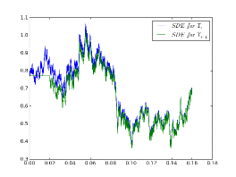
Figure 1: Behaviour of numerical paths of (1) when the appropriate coupling is used

This property implies that the variance of

$$\Delta^{(i,l)}:=g\left(\theta_{\frac{T_{l-1}}{h_{l-1}}}^{(f,l,i)}\right)-g\left(\theta_{\frac{T_{l-1}}{h_{l-1}}}^{(c,l,i)}\right)$$

for suitably chosen $T_{l-1}$ would remain small, thus allowing an application of the MLMC methodology. We will drop $i$ appropriately.

3.1 Multi-level SGLD

As common in MLMC we couple fine and coarse paths through the Brownian increments, with a Brownian increment on a coarse path given as a scaled sum of increments on the fine - $\frac{1}{\sqrt{2}}\left(\xi_{k,1}+\xi_{k,2}\right)$, which can be written in our notation as

$$\left(\theta_{k+1}^{(f)},\theta_{k+1}^{(c)}\right)=\left(S_{h_{i},\tau_{k,2}^{(f)},\xi_{k,2}}\circ S_{h_{i},\tau_{k,1}^{(f)},\xi_{k,1}}(\theta_{k}^{(f)}),S_{h_{l-1},\tau_{k,1}^{(c)},\frac{1}{\sqrt{2}}\left(\xi_{k,1}+\xi_{k,2}\right)}(\theta_{k}^{(c)})\right).$$ (7)

One question that naturally occurs now is that if and how should one choose to couple between the subsampling of the data? In particular, in order for the telescopic sum to be respected, one needs to have that the laws of distribution for subsampling the data is the same, namely

$$\mathcal{L}\left(\tau^{(f,1)}\right)=\mathcal{L}\left(\tau^{(f,2)}\right)=\mathcal{L}\left(\tau^{(c)}\right).$$ (8)

In order for this condition to hold we first take $s$ independent samples $\tau^{(f,1)}$ on the first fine-step and another $s$ independent s-samples $\tau^{(f,2)}$ on the second fine-step. In order to ensure that Equation 8 holds, we create $\tau^{(c)}$ by drawing $s$ samples without replacement from $\left(\tau^{(f,1)},\tau^{(f,2)}\right)$. Other strategies are also possible and we refer the reader to [18].

1. The initial steps are characterised by $\hat{s}_{l}=\frac{T_{l}-T_{l-1}}{h_{l}}$

2. set $\theta_{0}^{(c,l)}=\theta_{0}$ and $\theta_{0}^{(f,l)}=S_{h_{l},\tau_{-\hat{s}_{l}:-1},\xi_{-\hat{s}_{l}:-1}}$, then simulate $(\theta_{\cdot}^{(f,l)},\theta_{\cdot}^{(c,l)})$ jointly according to

   $$\left(\theta_{k+1}^{(f,l)},\theta_{k+1}^{(c,l)}\right)=\left(S_{h_{i},\tau_{k,2}^{(f)},\xi_{k,2}}\circ S_{h_{i},\tau_{k,1}^{(f)},\xi_{k,1}}(\theta_{k}^{(f,l)}),S_{h_{l-1},\tau_{k,1}^{(c)}\frac{1}{\sqrt{2}}\left(\xi_{k,1}+\xi_{k,2}\right)}(\theta_{k}^{(c,l)})\right).$$ (9)

   and set

   $$\Delta^{(i,l)}:=g\left(\theta_{s_{l-1}-k}^{(f,l)}\right)-g\left(\theta_{s_{l-1}-k}^{(c,l)}\right).$$

Algorithm 1 ML-SGLD for $t_{i}\uparrow\infty$

3.2 Antithetic Multi-level SGLD

Here we present the most promising variant of coupling on subsampling: Algorithm 2 for $t_{i}\uparrow\infty$. Building on the ideas developed in [11] (see also [10]) we propose Antithetic Multi-level SGLD which achieves an MSE of order complexity $\mathcal{O}(c^{-\frac{1}{2}})$ for prescribed computational cost (and therefore allows for MLMC with random truncation see [1]).

1. The initial steps are characterised by $\hat{s}_{l}=\frac{T_{l}-T_{l-1}}{h_{l}}$

2. set $\theta_{0}^{(c+,l)}=\theta_{0}^{(c-,l)}=\theta_{0}$ and $\theta_{0}^{(f,l)}=S_{h_{l},\tau_{-\hat{s}_{l}:-1}},\xi_{-\hat{s}_{l}:-1}$, then simulate $(\theta_{\cdot}^{(f,l)},\theta_{\cdot}^{(c,l)})$ jointly according to

   $$\begin{aligned} \theta_{k+1}^{(f,i)}&=S_{h_{l},\tau_{k,2},\xi_{k,2}^{(f)}}\circ S_{h_{i},\tau_{k,1}^{(f)},\xi_{k,1}}(\theta_{k}^{(f,l)})\\ \theta_{k+1}^{(c+,l)}&=,S_{h_{l-1},\tau_{k,1}^{(f,1)}\frac{1}{\sqrt{2}}\left(\xi_{k,1}+\xi_{k,2}\right)}(\theta_{k}^{(c,l)})\\ \theta_{k+1}^{(c-,l)}&=,S_{h_{l-1},\tau_{k,1}^{(f,2)}\frac{1}{\sqrt{2}}\left(\xi_{k,1}+\xi_{k,2}\right)}(\theta_{k}^{(c,l)})\end{aligned}$$ (10)

3. set

   $$\Delta^{(i,l)}:=g\left(\theta_{\frac{t_{l-1}}{h_{l-1}}-k}^{(f,l)}\right)-\frac{1}{2}\left(g\left(\theta_{\frac{t_{l-1}}{h_{l-1}}-k}^{(c+,l)}\right)+g\left(\theta_{\frac{t_{l-1}}{h_{l-1}}-k}^{(c-,l)}\right)\right).$$

Algorithm 2 Antithetic ML-SGLD for $t_{l}\uparrow\infty$

3.3 Averaging the Path

Compared to MCMC these algorithms seem wasteful because only the last step of a long simulation is saved. The numerical performance can be improved by instead averaging of parts of the trajectory as follows

$$\Delta_{\text{averaged}}^{(i,l)}:=\frac{1}{p_{l}}\sum_{k=0}^{p_{l}}g\left(\theta_{\frac{t_{l-1}}{h_{l-1}}-k}^{(f,l)}\right)-\frac{1}{p_{l-1}}\sum_{k=0}^{p_{l-1}}g\left(\theta_{\frac{t_{l-1}}{h_{l-1}}-k}^{(c,l)}\right),$$

and this also applies appropriately to the antithetic version.

3.4 Taylor based Stochastic Gradient

The idea of Taylor based stochastic gradient is to use subampling on the remainder of a Taylor approximation

$$\sum_{i=1}^{N}\nabla\log p\left(x_{i}|\theta\right)$$

$$=\sum_{i=1}^{N}\nabla\log p\left(x_{i}|\theta_{0}\right)+\sum_{i=1}^{N}\nabla^{2}\log p(x_{i}|\theta_{0})\left(\theta-\theta_{0}\right)$$

$$+\sum_{i=1}^{N}\left(\nabla\log p\left(x_{i}|\theta\right)-\left(\nabla\log p\left(x_{i}|\theta_{0}\right)+\nabla^{2}\log p(x_{i}|\theta_{0})\left(\theta-\theta_{0}\right)\right)\right)$$

$$\approx\sum_{i=1}^{N}\nabla\log p\left(x_{i}|\theta_{0}\right)+\left(\sum_{i=1}^{N}\nabla^{2}\log p(x_{i}|\theta_{0})\right)\left(\theta-\theta_{0}\right)$$ (11)

$$+\frac{N}{n}\sum_{i=1}^{n}\left(\nabla\log p\left(x_{\tau_{i}}|\theta\right)-\left(\nabla\log p\left(x_{\tau_{i}}|\theta_{0}\right)+\nabla^{2}\log p(x_{\tau_{i}}|\theta_{0})\left(\theta-\theta_{0}\right)\right)\right).$$

We expect that the Taylor based stochastic gradient to have small variance for $\theta-\theta_{0}$ small. The idea of subsampling the remainder originally was introduced in [2]. By interopolating between the Taylor based stochastic gradient and the standard stochastic gradient we have the best of both worlds.

4 Experiments

We use Bayesian logistic regression as testbed for our newly proposed methodology and perform a simulation study. The data $y_{i}\in\{-1,1\}$ is modelled by

$$p(y_{i}|\iota_{i},x)=f(y_{i}x^{t}\iota_{i})$$ (12)

where $f(z)=\frac{1}{1+\exp(-z)}\in[0,1]$ and $\iota_{i}\in\mathbb{R}^{d}$ are fixed covariates. We put a Gaussian prior $\mathcal{N}(0,C_{0})$ on $x$, for simplicity we use $C_{0}=I$ subsequently. By Bayes’ rule the posterior $\pi$ satisfies

$$\pi(x)\propto\exp\left(-\frac{1}{2}\left\|x\right\|_{C_{0}}^{2}\right)\prod_{i=1}^{N}f(y_{i}x^{T}\iota_{i}).$$

We consider $d=3$ and $N\in\{100,316,1000,3162,10000\}$ data points and choose the covariate to be

$$\iota=\left(\begin{array}[]{ccc}\iota_{1,1}&\iota_{1,2}&1\\ \iota_{2,1}&\iota_{2,2}&1\\ \vdots&\vdots&\vdots\\ \iota_{N,1}&\iota_{N,2}&1\end{array}\right)$$

for a fixed sample of $\iota_{i,j}\overset{\text{i.i.d.}}{\sim}\mathcal{N}\left(0,1\right)$ for $i=1,\dots N$ and we take $n=\left\lceil N^{\frac{1}{3}}\right\rceil$.

It is reasonable to start the path of the individual SGLD trajectories at a mode of the target distribution. This means that we set the $x_{0}$ to be the map estimator

$$x_{0}=\text{argmax}\>\exp\left(-\frac{1}{2}\left\|x\right\|_{C_{0}}^{2}\right)\prod_{i=1}^{N}f(y_{i}x^{T}\iota_{i})$$

which is approximated using the Newton-Raphson method. In the following we disregard the cost for the preliminary computations which could be reduced using state of the art optimisation and evaluating the Hessian in parallel. In the following we use MCMC and the newly developed MLSGLD to estimate the averaged squared distance from the map estimator under the posterior $\int_{\mathbb{R}^{3}}\|\theta-\theta_{0}\|^{2}\pi(x)dx$ i.e. set

$$g(\theta)=\|\theta-\theta_{0}\|^{2}.$$ (13)

Notice that by posterior consistency properties we expect this quantity to be have like $\frac{1}{N}$ which is why we will consider relative MSE.

4.1 Illustration of Coupling standard, antithetic and with Taylor

We choose $T_{l}=m(l+1)h_{0}$, $h_{l}=2^{-l}$ and leave $m\in\mathbb{N}$ as a tuning parameter. The crucial ingredient here is that in expectation the coarse and fine paths get closer exponentially initially and then asymptote, with the asymptote decaying as the step size decays. This illustrated on Figure 2a. As any MLMC algorithm performance is effected by the order $\beta$ of the variance $\mathrm{Var}\Delta^{(i,l)}\preceq h_{l}^{\beta}$, the parameters $m$ and $h_{0}$ should be chosen such that the difference between pathes reaches the asymptote, but preferrably does not spent to much time in it, as this increases the computational cost of sampling those paths. In our experiments we set $m=5$ and $h_{0}=1/N$ and on Figure 2c we see, that Algorithm 2 provides better coupling with variance decay of order $2$, which is significantly better than the first order variance decay, given by Algorithm 1. Combining Algorithm 2 with Taylor based extension from Section 3.4 and path averaging with $p_{l}=s_{l}/2$ from Section 3.3 gives additional decrease for the variance without affecting the rate $2$. The faster variance decay leads to lower overall complexity, as the number of samples at each level is proportional to the variance at that level. The Taylor Mean decay rates are of the same order, which can be seen on Figure 2b, but once again Algorithm 2 combined with Taylor and path averaging is more preferable, as the multiplicative constant is lower, than in Algorithm 1.

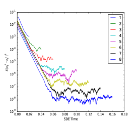
(a) Coupled levels

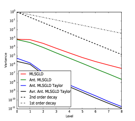
(b) Variance decay

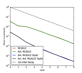
(c) Mean decay

Figure 2: Coupled paths at differen levels, variance and mean decays with respect to the levels.

Numerical evidence, presented here, leads to the conclusion, that Antithetic MLSGLD with Taylor along with Antithetic MLSGLD with Taylor and Averaging are the best competitors to MCMC algorithm, so we proceed to comparison of those algorithms.

4.2 Comparison with MCMC

We choose Metropolis-Adjusted Langevin (MALA, see [17]) as a competitor because it is based on one Euler step of the Langevin SDE, but adds a Metropolis accept-reject step in order to preserve the correct invariant measure (removing the requirement to decrease step size for better accuracy). We take cost as the number of evaluation of data items, which is typically measured in epochs. One epoch corresponds to one effective iteration through the full data set. Heuristically, for this log-concave problem we expect the convergence rate to be independent of $N$, so the only cost increase is due to evaluating posterior density and evaluating $\nabla\log\pi(X|\theta)$. This agrees with the findings in Figure 3a, where the MCMC lines are almost on top of each other thus yielding the same relative MSE for the same number of epochs for different dataset sizes. As $N$ increases the cost per epoch increases proportional to $N$. We run the MALA for $10^{4}$ steps with $10^{3}$ steps of burning and optimal acceptance rate $0.574$ for 50 times and then average. The various MLSGLD algorithms are ran for 50 times to achieve relative accuracies $2^{-k/2},\ k=2,\ldots,10$. This is yet another advantage of MLMC paradigm, which allows us to control numerically the mean increments and variance at all the levels, thus stopping the algorithm, when it has converged numerically.

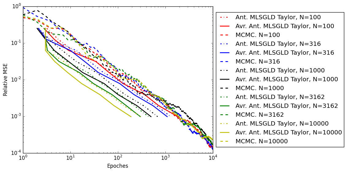
(a) Comparison of Mean Squared Relative Errors

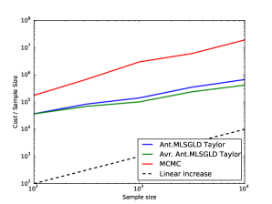
(b) Increase in Complexity

Figure 3: . Scalability of the algorithms and achieved Relative MSE for for differen datasets.

The most important comparison is presented on Figure 3b, where we compare the increase of the complexity to achieve relative accuracy of $2^{-5}$ with respect to the dataset size. We observe the sublinear growth of cost w.r.t dataset size for Antithetic MLSGLD with Taylor and Antithetic MLSGLD with Taylor and averaging, with the later having a slightly better behaviour than the first one.

5 Conclusion

We develop a Multilevel SGLD algorithm with computational complexity of $\mathcal{O}(c^{-\frac{1}{2}})$, hence closing the gap between MCMC and stochastic gradient methods. Moreover, this algorithm scales sublinearly with respect to the dataset size and allows natural parallelization, due to the typical properties of Monte Carlo sampling. The benefits of parallelization are to be studied later along with further numerical investigations for adaptive choices of parameters in the algorithm. In our further studies we also plan to quantify analytically the gains, given by MLSGLD algorithm and extend its applicability to a larger class of models.

References

- [1] S. Agapiou, G. O. Roberts, and S. J. Vollmer. Unbiased Monte Carlo: posterior estimation for intractable/infinite-dimensional models. arXiv preprint, 2014. To appear in Bernoulli.
- [2] C. Andrieu and S. Yildirim. Facilitating the penalty method for mcmc with large data. 2015.
- [3] R. Bardenet, A. Doucet, and C. Holmes. On Markov chain Monte Carlo methods for tall data. ArXiv e-prints, May 2015.
- [4] T. Chen, E. Fox, and C. Guestrin. Stochastic gradient Hamiltonian Monte Carlo. In Proc. International Conference on Machine Learning, June 2014.
- [5] N. Ding, Y. Fang, R. Babbush, C. Chen, R. D. Skeel, and H. Neven. Bayesian sampling using stochastic gradient thermostats. In Z. Ghahramani, M. Welling, C. Cortes, N. Lawrence, and K. Weinberger, editors, Advances in Neural Information Processing Systems 27, pages 3203–3211. Curran Associates, Inc., 2014.
- [6] S. Duane, A. Kennedy, B. J. Pendleton, and D. Roweth. Hybrid monte carlo. Physics Letters B, 195(2):216 – 222, 1987.
- [7] A. Durmus and E. Moulines. Non-asymptotic convergence analysis for the Unadjusted Langevin Algorithm. ArXiv e-prints, July 2015.
- [8] A. Eberle. Reflection coupling and wasserstein contractivity without convexity. Comptes Rendus Mathematique, 2011.
- [9] M. B. Giles. Multilevel Monte Carlo path simulation. Oper. Res., 2008.
- [10] M. B. Giles. Multilevel Monte Carlo methods. Acta Numer., 24:259–328, 2015.
- [11] M. B. Giles and L. Szpruch. Antithetic multilevel Monte Carlo estimation for multi-dimensional SDEs without Lévy area simulation. Ann. Appl. Probab., 24(4):1585–1620, 2014.
- [12] M. Girolami and B. Calderhead. Riemann manifold langevin and hamiltonian monte carlo methods. Journal of the Royal Statistical Society: Series B (Statistical Methodology), 73(2):123–214, 2011.
- [13] P. W. Glynn and C.-H. Rhee. Exact estimation for markov chain equilibrium expectations. J. Appl. Probab., 51A:377–389, 12 2014.
- [14] A. Kebaier. Statistical Romberg extrapolation: a new variance reduction method and applications to option pricing. Ann. Appl. Probab., 15(4):2681–2705, 2005.
- [15] B. Leimkuhler and X. Shang. Adaptive thermostats for noisy gradient systems. SIAM Journal on Scientific Computing, 38(2):A712–A736, 2016.
- [16] R. M. Neal. MCMC using Hamiltonian dynamics. Handbook of Markov Chain Monte Carlo, 54:113–162, 2010.
- [17] G. O. Roberts and R. L. Tweedie. Exponential convergence of langevin distributions and their discrete approximations. Bernoulli, pages 341–363, 1996.
- [18] L. Szpruch, S. Vollmer, K. C. Zygalakis, and M. B. Giles. Multi level monte carlo methods for a class of ergodic stochastic differential equations. arXiv:1605.01384.
- [19] Y. W. Teh, A. H. Thiery, and S. J. Vollmer. Consistency and fluctuations for stochastic gradient langevin dynamics. Journal of Machine Learning Research, 17(7):1–33, 2016.
- [20] Y. W. Teh, S. J. Vollmer, and K. C. Zygalakis. (Non-) asymptotic properties of stochastic gradient langevin dynamics. ArXiv e-prints, 2015.
- [21] M. Welling and Y. W. Teh. Bayesian Learning via Stochastic Gradient Langevin Dynamics. In Proceedings of the 28th ICML, 2011.