Time Derivative of Rotation Matrices: A Tutorial

Abstract

The time derivative of a rotation matrix equals the product of a skew-symmetric matrix and the rotation matrix itself. This article gives a brief tutorial on the well-known result.

I Introduction

The attitude of a ground or aerial robot is often represented by a rotation matrix, whose time derivative is important to characterize the rotational kinematics of the robot. It is a well-known result that the time derivative of a rotation matrix equals the product of a skew-symmetric matrix and the rotation matrix itself. One classic method to derive this result is as follows [1, Sec 4.1], [2, Sec 2.3.1], and [3, Sec 4.2.2] (see [4] for other methods). Let $R(t)\in\mathbb{R}^{3\times 3}$ with $t\geq 0$ be a rotation matrix satisfying $R(t)R^{\mathrm{T}}(t)=I$ for all $t$ where $I$ is the identity matrix. Taking time derivative on both sides of $R(t)R^{\mathrm{T}}(t)=I$ gives

$$\dot{R}(t)R^{\mathrm{T}}(t)+R(t)\dot{R}^{\mathrm{T}}(t)=0,$$

which indicates that $S(t)\triangleq\dot{R}(t)R^{\mathrm{T}}(t)$ is a skew-symmetric matrix satisfying $S(t)+S^{\mathrm{T}}(t)=0$ for all $t$, and consequently

$$\dot{R}(t)=S(t)R(t).$$

The above derivation is simple, but it is not straightforward to see the precise physical meaning of $S(t)$ (though $S(t)$ corresponds to an angular velocity vector, it is unclear which reference frame this vector is expressed in). This article gives another simple derivation, which is essentially a reorganization of the derivation in [1, 2, 3], to clarify the precise physical meanings of the quantities in the expression of the time derivative of a rotation matrix.

Notation: For any vector $w=[w_{1},w_{2},w_{3}]^{\mathrm{T}}\in\mathbb{R}^{3}$, define the skew-symmetric operator $\left[\cdot\right]_{\times}$ as

$$\left[w\right]_{\times}\triangleq\left[\begin{array}[]{ccc}0&-w_{3}&w_{2}\\ w_{3}&0&-w_{1}\\ -w_{2}&w_{1}&0\\ \end{array}\right]\in\mathbb{R}^{3\times 3}.$$ (4)

The skew-symmetric operator is useful because it can convert a cross product of two vectors into a matrix-vector product. More specifically, for any $w,x\in\mathbb{R}^{3}$, it can be easily verified that $w\times x=\left[w\right]_{\times}x$. Another useful property is that for any $w\in\mathbb{R}^{3}$ and any rotation matrix $R\in\mathbb{R}^{3\times 3}$ satisfying $RR^{\mathrm{T}}=I$ and $\det(R)=1$ it holds that $\left[Rw\right]_{\times}=R\left[w\right]_{\times}R^{\mathrm{T}}$ [3, Section 4.2.1].

II Time Derivative of Rotation Matrices

Consider two reference frames $A$ and $B$ in the three-dimensional space (see Figure 1). Assume the origins of the two frames collocate with each other. Suppose frame $A$ is fixed and frame $B$ is rotating. In the area of robotics, frame $A$ usually corresponds to the world frame fixed on the ground, and frame $B$ usually corresponds to the body frame attached to the body of a robot.

Figure 1: Frame $A$ is fixed while frame $B$ is rotating.

In the sequel, the time variables of all the matrices and vectors are omitted for the sake of simplicity. Let the rotation matrix $R_{B}^{A}\in\mathbb{R}^{3\times 3}$, which satisfies $(R_{B}^{A})^{-1}=(R_{B}^{A})^{\mathrm{T}}$ and $\det(R_{B}^{A})=1$, represent the rotational transformation from frame $B$ to frame $A$. For any point in the space, suppose $P_{A}\in\mathbb{R}^{3}$ and $P_{B}\in\mathbb{R}^{3}$ are its coordinates expressed in frames $A$ and $B$, respectively, then

$$P_{A}=R_{B}^{A}P_{B}.$$

Let $R_{A}^{B}=(R_{B}^{A})^{\mathrm{T}}$ be the rotation from frame $A$ to frame $B$.

Suppose $w_{B}\in\mathbb{R}^{3}$ is the angular velocity of frame $B$ (relative to frame $A$) expressed in frame $B$. The vector $w_{B}$ quantifies the rotational movement of frame $B$: $\|w_{B}\|$ equals to the angular rate, which quantifies how fast frame $B$ is rotating, and $w_{B}/\|w_{B}\|$ indicates the axis of the rotational movement. Since the angular velocity is a vector, it can also be expressed in frame $A$ as $w_{A}\in\mathbb{R}^{3}$, which satisfies

$$w_{A}=R_{B}^{A}w_{B}.$$

The following is the main result on the relation between rotational transformations and angular velocities.

Theorem 1 (Time Derivative of Rotation Matrices).

The time derivative of the rotational transformations $R_{B}^{A}$ and $R_{A}^{B}$ are expressed as

$$\dot{R}_{B}^{A} =[w_{A}]_{\times}R_{B}^{A}$$ (5)

$$\dot{R}_{B}^{A} =R_{B}^{A}[w_{B}]_{\times}$$ (6)

$$\dot{R}_{A}^{B} =-R_{A}^{B}[w_{A}]_{\times}$$ (7)

$$\dot{R}_{A}^{B} =-[w_{B}]_{\times}R_{A}^{B}$$ (8)

Proof.

We first prove (5). Consider an arbitrary point fixed in frame $B$. If $P_{A}$ and $P_{B}$ are the coordinates of this point in frames $A$ and $B$, respectively, then $P_{B}$ is constant since the point is fixed in frame $B$, and $P_{A}$ is time-varying since frame $B$ is rotating. As a result, we have $\dot{P}_{B}=0$. Taking time derivative on both sides of $P_{A}=R_{B}^{A}P_{B}$ yields

$$\dot{P}_{A}=\dot{R}_{B}^{A}P_{B}.$$ (9)

On the other hand, by the relation between linear and angular velocities, we have

$$\dot{P}_{A}=w_{A}\times P_{A}=[w_{A}]_{\times}P_{A}.$$ (10)

Substituting (10) into (9) gives

$$\dot{R}_{B}^{A}P_{B}=[w_{A}]_{\times}P_{A}=[w_{A}]_{\times}R_{B}^{A}P_{B}.$$ (11)

Since $P_{B}$ may be arbitrarily chosen, equation (11) holds for arbitrary $P_{B}\in\mathbb{R}^{3}$ and hence implies (5).

Equations (6)–(8) can be derived from (5). In particular, by the property of the skew-symmetric operator, we have

$$\left[w_{A}\right]_{\times}=\left[R_{B}^{A}w_{B}\right]_{\times}=R_{B}^{A}\left[w_{B}\right]_{\times}(R_{B}^{A})^{\mathrm{T}}.$$ (12)

Substituting (12) into (5) yields $\dot{R}_{B}^{A}=\left[w_{A}\right]_{\times}R_{B}^{A}=R_{B}^{A}\left[w_{B}\right]_{\times}(R_{B}^{A})^{\mathrm{T}}R_{B}^{A}=R_{B}^{A}\left[w_{B}\right]_{\times}$, which is (6). Taking transpose on both sides of (5) gives $\dot{R}_{A}^{B}=-R_{A}^{B}\left[w_{A}\right]_{\times}$, which is (7). By substituting (12) into (7) leads to (8). ∎

As indicated by Theorem 1, the expression of the time derivative depends on the definitions of the rotation transformation and angular velocity. One should be clear about their physical meanings before applying (5)–(8).

III Practical Consideration in Robotic Motion

For a robot equipped with an inertial measurement unit (IMU), the value of $w_{B}$, which is the angular velocity of the robot relative to the world frame expressed in its body frame, can be directly measured. As a result, equations (6) and (8), i.e.,

$$\dot{R}_{B}^{A} =R_{B}^{A}[w_{B}]_{\times}$$

$$\dot{R}_{A}^{B} =-[w_{B}]_{\times}R_{A}^{B}$$

are particularly useful in practice.

It must be noted that the origins of frames $A$ and $B$ are assumed to collocate with each other in Theorem 1. This assumption is, however, usually not satisfied for moving robots because the body frame may translate in the space (see Figure 2). Nevertheless, (6) and (8) still holds in this case. To prove that, we may introduce an intermediate frame $A^{\prime}$ whose axes are parallel to those of frame $A$ and origin collocates with the origin of frame $B$. By considering frames $A^{\prime}$ and $B$, we have $\dot{R}_{B}^{A^{\prime}}=R_{B}^{A^{\prime}}[w_{B}]_{\times}$ and $\dot{R}_{A^{\prime}}^{B}=-[w_{B}]_{\times}R_{A^{\prime}}^{B}$. Since the axes of frame $A^{\prime}$ are parallel to those of frame $A$, we always have $R_{B}^{A^{\prime}}=R_{B}^{A}$ and $R_{A^{\prime}}^{B}=R_{A}^{B}$ and consequently (6) and (8) still holds (note $w_{B}$ remain the same). On the other hand, if the origins of frames $A$ and $B$ do not collocate, equations (5) and (7) do not hold any more because $w_{A}^{\prime}\neq w_{A}$ due to the nonzero translation between frames $A^{\prime}$ and $A$. With the above discussion, we know equations (6) and (8) are more useful than equations (5) and (7) in practice.

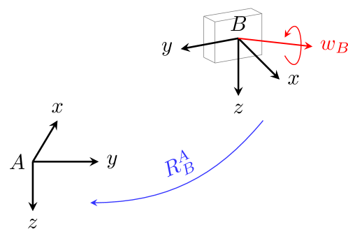
Figure 2: The world frame $A$ and body frame $B$ for a robot moving in the three-dimensional space.

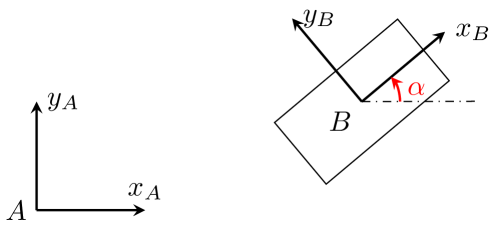
Figure 3: The world frame $A$ and body frame $B$ for a robot moving in the plane.

If a robot is moving in the plane, the rotation (or orientation) of the robot can be represented by a single angle $\alpha$ (see Figure 3). Then, the rotation transformation from frame $B$ to frame $A$ is

$$R_{\alpha}=\left[\begin{array}[]{cc}\cos\alpha&-\sin\alpha\\ \sin\alpha&\cos\alpha\\ \end{array}\right].$$

In order to verify $R_{\alpha}$, one may examine some specific points in frame $B$ such as $e_{1}=[1,0]^{\mathrm{T}}$ and $e_{2}=[0,1]^{\mathrm{T}}$. Taking time derivative on both sides of $R_{\alpha}$ gives

$$\dot{R}_{\alpha}=\left[\begin{array}[]{cc}-\sin\alpha&-\cos\alpha\\ \cos\alpha&-\sin\alpha\\ \end{array}\right]\dot{\alpha}.$$ (15)

Expression (15) may also be obtained as a special case of (6). In particular, we can consider the three-dimensional frame with the $z$-axes pointing out of the paper in Figure 3. Then,

$$R_{B}^{A}=\left[\begin{array}[]{ccc}\cos\alpha&-\sin\alpha&0\\ \sin\alpha&\cos\alpha&0\\ 0&0&1\\ \end{array}\right].$$

The angular velocity of the robot can be expressed as $w_{A}=w_{B}=\dot{\alpha}e_{3}$ where $e_{3}=[0,0,1]^{\mathrm{T}}$. By applying (5) or (6), it is straightforward to obtain (15).

References

• [1] R. M. Murray, Z. Li, and S. S. Sastry, A Mathematical Introduction to Robotic Manipulation. CRC Press, 1994.
• [2] Y. Ma, S. Soatto, J. Kosecka, and S. Sastry, An Invitation to 3D Vision. New York: Springer, 2004.
• [3] M. W. Spong, S. Hutchinson, and M. Vidyasagar, Robot Modeling and Control. John Wiley & Sons, Inc., 2006.
• [4] F. Hamano, “Derivative of rotation matrix - direct matrix derivation of well-known formula,” in Proceedings of Green Energy and Systems Conference, (Long Beach, CA), 2013.