Evidence of asymmetries in the Aldebaran photosphere from multi-wavelength lunar occultations

Abstract

We have recorded three lunar occultations of Aldebaran ($\alpha$ Tau) at different telescopes and using various band-passes, from the ultraviolet to the far red. The data have been analyzed using both model-dependent and model-independent methods. The derived uniform-disc angular diameter values have been converted to limb-darkened values using model atmosphere relations, and are found in broad agreement among themselves and with previous literature values. The limb-darkened diameter is about 20.3 milliarcseconds on average . However, we have found indications that the photospheric brightness profile of Aldebaran may have not been symmetric, a finding already reported by other authors for this and for similar late-type stars. At the sampling scale of our brightness profile, between one and two milliarcsecond, the uniform and limb-darkened disc models may not be a good description for Aldebaran. The asymmetries appear to differ with wavelength and over the 137 days time span of our measurements. Surface spots appear as a likely explanation for the differences between observations and the models.

1 Introduction

Aldebaran ($\alpha$ Tau) is one of the brightest and most distinctive stars in the sky, and as a result it has one of the longest records of observations and publications. Being a K5 giant star and located at just 20 pc from the Sun, it has also one of the largest angular diameters among all stars and it has therefore been the subject of numerous measurements in this sense using a number of techniques. Since Aldebaran is located on the Zodiac, it is regularly occulted by the Moon. We are at present in the middle of one such series of occultations, which will last until early 2018.

Richichi & Roccatagliata (2005, RR05 hereafter) presented accurate lunar occultation (LO) and long-baseline interferometry measurements obtained in the near-infrared, and discussed them in the context of previously available determinations. They concluded that the limb-darkened diameter of $\alpha$ Tau is $20.58\pm 0.03$ milliarcseconds (mas), or 44 $R_{\odot}$. Photometric variability is less than 0.01 mag and the diameter is assumed to be reliably constant. Differences in the angular diameter values available in the literature are indeed present and sometimes significant when taken at face value, however they can often be justified in terms of uniform disc to limb-darkening corrections or by intrinsic limitations in the accuracy.

We have recorded three LO events in the present series, and we present here their detailed analysis. Our aim is not so much to confirm or refine the angular diameter determination, but rather to investigate possible asymmetries or surface structure features in the photosphere of this giant star. Indications in this sense had already been presented by RR05.

2 Observations and Data Analysis

We recorded three LO light curves of $\alpha$ Tau: in October 2015 using the SAO 6-m telescope in Russia, and in March 2016 using the Devasthal 1.3-m telescope in India and the TNT 2.4-m telescope in Thailand. Details of the observations are provided in Table 1.

Table 1: Observations log

Telescope	SAO 6-m	1.3-m	TNT 2.4-m
Site	Nizhny Arkhyz, Russia	Devasthal, India	Doi Inthanon, Thailand
Coordinates	41$\degr$26$\arcmin$E, 43$\degr$39$\arcmin$N, 2100m	79$\degr$41$\arcmin$E, 29$\degr$22$\arcmin$N, 2450m	98$\degr$29$\arcmin$E, 18$\degr$34$\arcmin$N, 2450m
Date, Time (UT)	2015-10-29, 23:32:01	2016-03-14, 14:40:29	2016-03-14, 15:15:32
Event	Reappearance	Disappearance	Disappearance
Predicted PA, Rate	229$\degr$,$-$0.616 m/ms	99$\degr$, 0.732 m/ms	125$\degr$, 0.734 m/ms
Detector	ANDOR	ANDOR	ULTRASPEC
Filter ($\lambda$, $\Delta\lambda$) (nm)	Filterless	R (640, 130)	$u\arcmin$ (356, 60)
$\lambda_{\rm eff}$ (nm)	752	644	371
Sampling (ms)	2.58	1.85	6.29
CAL, DIF Sampling (mas)	0.90	0.76	2.57

At SAO, a commercial 512x512 pixels Andor iXon Ultra DU-897-CS0 detector was used. For this observation we used binning 16x16, readout rate 17 MHz, electron multiplying gain = 100, shift speed = 0.5 $\mu$s, 0.1 ms exposure time, kinetic regime. This resulted in a kinetic cycle time of 2.58 ms. The readout noise at this rate was 93 e^-.The result was a FITS data cube, with 32x32 pixel size and 150,000 frames. At Devasthal, a similar detector was used, namely a 512x512 pixels frame transfer ANDOR iXon EMCCD (DU-897E-CS0-UVB-9DW). For this observation, the central 32x32 pixels were used in 2x2 binning mode. Readout rate 10 MHz, shift speed 0.9 $\mu$s, 1.38 ms exposure time resulted in a kinetic cycle time of 1.85 ms. The final image was a FITS data cube containing 45,000 frames. At TNT, we used the ULTRASPEC frame-transfer EMCCD imager (Dhillon et al., 2014) in the so-called drift mode already used previously for LO (Richichi et al., 2014, 2016). We used a window of 8x8 pixels ($3\aas@@fstack{\prime\prime}6$ x $3\aas@@fstack{\prime\prime}6$ on the sky), and a SDSS $u\arcmin$ filter. The resulting FITS data cube consisted of 9371 frames, with sampling time of 6.288 ms and integration time of 6.123 ms.

In all three cases, we built an effective wavelength response of the instrument by convolving the filter with the CCD quantum efficiency and the optics. The effective (weighted average) wavelengths $\lambda_{\rm eff}$ for each case are listed in Table 1. We also included in our analysis the effects of the finite integration time, and of the primary diameter and obstruction.

The data cubes were trimmed to include only a few seconds around the occultation event, and converted to light curves using a mask extraction tailored to the seeing and image motion, as described in Richichi et al. (2008). The light curves were then analyzed using several methods. Firstly, a least-square model-dependent (LSM) analysis was used, the details of which are given in Richichi et al. (1992). This approach uses a uniform-disc (UD) model of the stellar disc with its angular diameter as a free parameter, and achieves convergence in $\chi^{2}$ based a noise model built from data before and after the occultation. Among other parameters, this method allows to determine in principle also the actual slope of the lunar limb from the comparison between predicted and fitted lunar rate. However, in the specific case of a large angular diameter such as that of $\alpha$ Tau all diffraction fringes except at the most the first one (see below) are almost completely erased, and this benefit of the LSM method cannot be realized (see also Sect. 3.1). Additionally, although our implementation of the LSM method allows in principle to partly account for scintillation by means of interpolation by Legendre polynomials, for the same reason as above this cannot be done in practice for the $\alpha$ Tau LO data.

Secondly, we used a composite algorithm (CAL) which provides a model-independent brightness profile of the source in the maximum-likelihood sense (Richichi, 1989). Finally, we also used a simple differentiation (DIF) to reconstruct the brightness profile in a model-independent fashion. This latter method is applicable when the occultation can be described by simple geometrical optics. This is the case when the source angular diameter $\phi$, the wavelength $\lambda$ and the distance to the Moon D satisfy the relation $\phi>\sqrt{\lambda/{\rm D}}$. With an angular diameter of about 20 mas, Aldebaran satisfies this relationship marginally in the far red, and completely in the ultraviolet. The difference between the CAL and the DIF methods is that the first one modifies an initial brightness profiles with small steps during a large number of iterations (typically thousands), resulting in a relatively smooth profile; the second method, instead, performs a single differentiation operation but is affected by point-to-point noise in the data. This noise can be reduced by rebinning the data before differentiation, at the expense however of the final angular resolution.

With the LSM method, the achieved angular resolution is related to the time sampling but also to the quality of the fit (expressed by the normalized $\chi^{2}$ ) and the signal-to-noise ratio (SNR) of the data. In practice, this is the method which will yield the best resolution and accuracy, at least formally. For CAL and DIF, the resulting brightness profiles have a step in angular resolution which is related to the sampling time, to the apparent speed of motion of the lunar limb, and to the distance to the Moon. The theoretical angular sampling of the brightness profiles for these two methods are listed in Table 1. In case of data rebinning, the angular step of the CAL and DIF profiles will be reduced accordingly.

3 Results

The three data sets are shown in Fig. 1, rescaled and offset by arbitrary amounts to fit in a single, compact figure. Some aspects of the data can be appreciated prior to any quantitative analysis, such as for example the progressive transition from the diffraction to the geometrical regime. The SAO 6-m curve has a redder effective wavelength than the Devasthal 1.3-m curve, and indeed it shows a slightly more pronounced first fringe. It is however surprising that the TNT 2.4-m curve, which should be completely within the geometrical optics regime, appears to show in fact a diffraction fringe. It is also evident how the telescope diameter strongly affects the level of scintillation, as expected: with comparable wavelengths, the SAO 6-m data have indeed significantly lower scintillation than those from the Devasthal 1.3-m. In the remainder of this section, we report and illustrate the results of the quantitative data analysis of these curves, first by the model-dependent and then by the model-independent methods.

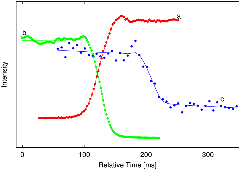
Figure 1: Light curves (points) marked as a, b, c, from the SAO 6-m, the Devasthal 1.3-m and the TNT 2.4-m telescopes, respectively. The data have been shifted in time, scaled and shifted in intensity, to fit in a single figure. The solid lines are the best fit by a uniform-disc (UD) model in each case, as discussed in the text.

3.1 Uniform- and Limb-Darkened Disc Diameter

We report on the data analysis using the LSM method first, the natural outcome of which is the best fitting angular diameter on the basis of a noise model built individually for each light curve and each instrument as detailed above. We assume a stellar model with a uniform disc (UD), since this is easily described by one parameter only, i.e. the angular size. In reality the star is generally better described in terms of a limb-darkened disc (LD). Although it is possible to describe LD brightness profiles analytically, this requires a number of additional parameters and in practice their effect on the fitting process is not sufficient to obtain well-determined values unless the light curve has a very high SNR. We thus follow the customary approach of determining UD diameters first. The results are listed in Table 2. We note that, due to the almost complete suppression of the diffraction fringes in the case of $\alpha$ Tau, the actual rate of the event is not a completely independent parameter as in other LO light curves of sources with smaller angular diameters. In fact, in this particular situation the rate is correlated to the angular size. For this reason, we have decided to keep the rate to its predicted value in the three fits. More comments about this are given in Sect. 4.

Table 2: Uniform and limb-darkened diameter values

Telescope	SAO 6-m	1.3-m	TNT 2.4-m
$\lambda_{\rm eff}$ (nm)	752	644	371
UD (mas)	19.12$\pm$0.02	18.40$\pm$0.04	17.78$\pm$0.38
SNR	165.5	65.3	11.4
Normalized $\chi^{2}$	1.21	1.76	0.94
(LD/UD)eff (see text)	1.07	1.09	1.15
LD (mas)	20.42$\pm$0.02	20.06$\pm$0.04	20.48$\pm$0.44

UD diameters are wavelength dependent, and as expected the three values listed in Table 2 do not agree with each other given the different band-passes. It can be however appreciated how the UD diameter value increases monotonically with $\lambda_{\rm eff}$. It can also be noted that the accuracy of the resulting diameter value is closely related to the SNR, as discussed in Sect. 2. In order to compare results obtained at various wavelengths and to test atmospheric models, it is useful to convert the wavelength-dependent UD values to their limb-darkened (LD) diameter equivalent.

It is customary to generate LD/UD coefficients from model atmospheres. Davis et al. (2000) derived detailed LD/UD coefficients as a function of wavelength for a large grid of stellar atmospheric models, based on the atlas distributed by R.L. Kurucz on CD-ROMs in 1993. The coefficients are tabulated in discrete steps of effective temperature T_eff, of surface gravity log $g$, and of metallicity Z=log [Fe/H]. For the temperature, we adopt the value T_eff=3920$\pm$15 K by Blackwell et al. (1991), which is in excellent agreement with the value of 3934$\pm$41 K derived by RR05. For log $g$, we adopt the value of 1.25$\pm$0.49 by Bonnell & Bell (1993). There are numerous other references for these quantities, but they generally agree within the errors with our adopted values. The metallicity of $\alpha$ Tau is quoted in the literature with a range of values ranging from solar to less than half solar (Cayrel de Strobel et al., 1992). Recently, Jofré et al. (2014) have analyzed the data available on the metallicity of a number of GAIA benchmark stars using several different methods. They find Z=$-0.37\pm 0.02$ for Aldebaran, and this is our adopted value as well.

We thus selected those curves among those provided by Davis et al. (2000) which bracket our adopted T_eff, log $g$ and Z, and proceeded to interpolate between them. The resulting LD/UD correction as a function of wavelength is shown in Fig.2. It can be noted that the Davis et al. (2000) data stop at $\lambda$=400 nm. Since our TNT observation extends to about $\lambda$=325 nm, we took the simple approach of extrapolating the curve, as also shown in Fig.2.

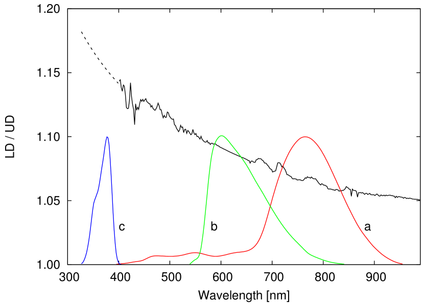
Figure 2: Solid curve: the monochromatic LD/UD coefficients, interpolated from the database of Davis et al (2005) for our assumed Aldebaran atmospheric parameters. Dashed curve: extrapolation below 400 nm. The three curves labeled a, b, c are shown in arbitrary vertical units: they represent the total transmission of the instruments at SAO, Devasthal, and TNT, respectively. They include the effects of CCD, optics and filter.

We note that as long as the LD/UD uncertainty is less than 0.03, which seems a reasonable upper limit also in the case of the ultraviolet extrapolation, the effect on the error in the LD diameter is less than the last digit shown in Table 2.

3.2 Applicability and Discrepancies of Disc Models

It must be remarked that the LD/UD coefficients are strictly applicable only for monochromatic wavelengths, while our data and thus our UD diameter results are for broad-band filters. To account for this, we have computed an effective LD/UD correction for each of the three LO cases, by weighing the LD/UD curve by the effective transmission of filter, CCD and optics, and normalizing. The results are listed in Table 2 as (LD/UD)_eff. Using these corrections, we derive LD diameter values which are also listed in Table 2. It can be seen that the LD values from SAO and TNT are consistent among themselves and in some agreement with the LD diameter of $20.58\pm 0.03$ mas reported by RR05 - although not within the errors in the case of the SAO result. The result from the Devasthal 1.3-m telescope however has to be considered discrepant.

To investigate further this apparent discrepancy, we have plotted in Fig. 3 the fit residuals (normalized in units of the light curve intensity) for the two light curves with the best quality, those from SAO and from Devasthal, in the central part where the intensity goes from unocculted to occulted. It can be noticed that the Devasthal data show a quasi-sinusoidal variation. Scintillation comes first to mind as a possible cause, but it would not be so regular and moreover its amplitude should be proportional to the stellar flux. The flux changes from full unocculted intensity at the left of Fig. 3, to zero at the right. Therefore, scintillation can be convincingly excluded as the cause of this beating in the residuals for the Devasthal curve. We note that in the case of the SAO data scintillation decreases from the right to the left of Fig. 3, and indeed one might see that the right part of the residuals appears slightly noisier.

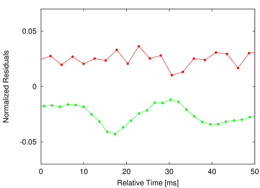
Figure 3: The fit residuals for the central part of the SAO and Devasthal light curves shown in Fig. 1, top and bottom respectively. The residuals have been normalized by the intensity of the unocculted source, and shifted vertically by $\pm 0.025$ units for clarity. They have also been shifted horizontally into a common time window.

We are inclined to conclude that the residuals indicate, at least in the Devasthal case, that the UD is not a good model at the level of the accuracy present in the data. The even higher accuracy data from SAO however do not show this effect with the same magnitude, and we can speculate that the UD (and LD as a consequence) model is a better approximation in the infrared part of the visible range. Another possible reason are time variable changes in the profile, which we discuss in Sect. 4. The case of the TNT data in the ultraviolet is harder to pin down from an analysis of the residuals, since the noise was so much higher in this case due to a combination of poorer combined throughput on one hand, and of much higher background on the other. However, we have already remarked that the TNT light curve shown in Fig. 1 seems to exhibit a first diffraction fringe which is totally unexpected since diffraction effects should have been negligible at this wavelength. One possible cause of such a fringe, if real, could be a compact area (about 20% of the diameter or less) of enhanced emission on the photosphere. The jagged ultraviolet brightness profiles discussed in Sect. 3.3 could point in this direction, although the errors make this far from conclusive.

3.3 Model-independent Brightness Profiles

LD diameters are ultimately the values which are employed in standard stellar atmospheric models, but they are the result of assumed empirical conversions which are not directly measured or confirmed by observations. Moreover, the extension from the monochromatic values to an effective conversion coefficient valid for a broad bandpass is prone to introduce a possible bias. Even more significantly, the whole issue of determining an accurate diameter depends on the chosen model brightness distribution which is assumed to be axisymmetric and constant with time. The discrepancies which we have highlighted in Sect 3.2 all point to cracks in these assumptions. In the case of Aldebaran however we are in the fortunate position to be able to reconstruct the brightness profile directly by model-independent methods.

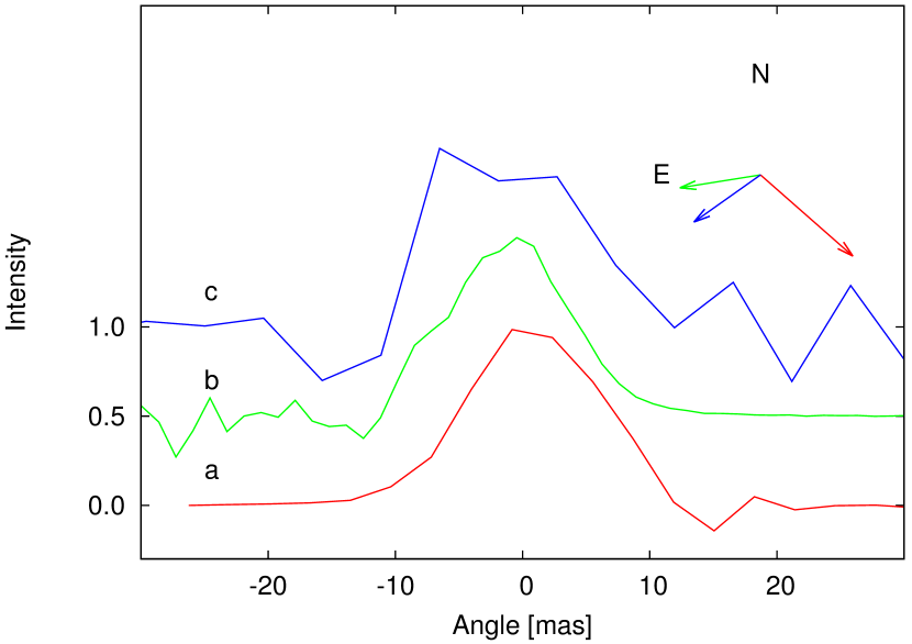
Figure 4: Reconstructed brightness profiles, using differentiation as explained in the text. The curves a, b, c, are for the data sets from SAO 6-m, Devasthal 1.3-m and TNT 2.4-m, respectively, with the effective wavelengths listed in Table 1. The profiles are shifted by arbitrary amounts in intensity, for the sake of clarity. The arrows display the direction of the scan by the lunar limb, projected on the sky and in counter-clockwise direction from the North they are for b, c, a respectively. The length of the arrows is inversely proportional to the speed of the scan.

Profiles reconstructed by the DIF method are shown in Fig. 4. By its design, this method is sensitive to white noise in the data and this explains why the profiles of the curves from SAO and India are noisier on the side where scintillation is affecting the data, the right and left sides of the respective profiles. In the case of TNT, the dominant source of noise is not scintillation but rather the shot-noise from the very intense background around the Moon in the ultraviolet, and it can be seen that the noise in the profile is more evenly distributed. Further, in all three cases a slight dip towards negative values of the profile is due to presence of small residual diffraction fringe in the light curves: this can be seen to the right of the SAO profile, and to the left in the other two cases. It can be appreciated how in all three cases the profile does not appear to be completely symmetric. In the case of the ultraviolet data from TNT, a relatively flat central part of the profile is present. Limb-brightening as observed in far-ultraviolet solar images comes to mind, although our SNR is not sufficient to confirm this hypothesis.

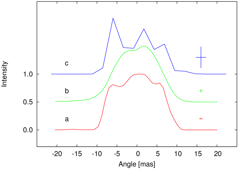
Figure 5: Reconstructed brightness profiles, using the maximum-likelihood CAL method as explained in the text. The curves are shifted in intensity, labeled and with the same sky orientation as in Fig. 4. The crosses on the right reflect the uncertainties for each profile, as explained in the text.

We have computed the profiles also by the CAL method, and they are shown in Fig. 5. The profiles are consistent with an approximate extent of 20 mas, but show structure which is markedly different from the gaussian shape expected for a circularly symmetric uniform disc (Richichi, 1989). In the figure we have added error crosses for each profile: the extent in angle is simply the sampling step from Table 1, while the extent in intensity is derived from the SNR of the CAL fit rescaled by the number of points inside the Aldebaran’s disc. To clarify: the total reconstructed SAO profile extended from $-50$ to $+40$ mas, and included 46 points with a SNR of 177.8, or an error of 0.0056 on the normalized intensity. The points effectively inside the $\pm 10$ mas extent of the disc are 22. Assuming that those outside the disc do not contribute significantly to the noise total, we compute the effective error in normalized intensity as $46/22\times 0.0056=0.012$.

To clarify how these profiles deviate from the expectation, we have analyzed three sources which are presumed from empirical considerations to be unresolved, with each of the three telescopes and instruments used also for $\alpha$ Tau - albeit in different filters. In Fig. 6 we show the CAL profiles obtained for 1 Cnc observed at SAO on February 19, 2016; for SAO 94227 observed at Devasthal on February 16, 2016; and for HR 4418 observed at TNT on April 18, 2016. We have also added a recent LO observation of $\lambda$ Aqr observed from SAO on June 25, 2016: this result will be discussed elsewhere, but it can be seen that the profile is very well resolved and represents a case not too dissimilar from that of $\alpha$ Tau. It can be appreciated that, at the level of the discrete angular sampling of the three data sets, the profiles do not show significant asymmetries, in contrast with those found for $\alpha$ Tau.

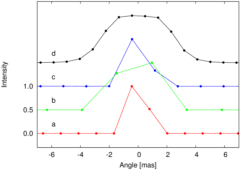
Figure 6: Same as Fig. 5, for three unresolved sources observed at SAO (a), Devasthal (b) and TNT (c). The curve (d) is for a well resolved star observed at SAO. The profiles do not display obvious asymmetries. The points mark the different angular sampling of the data sets. Details in the text.

We emphasize that DIF and CAL profiles should be used to investigate the general appearance of the brightness profiles only. They are not well suited to measure angular diameters since they are not parametric and because the angular scale depends on the adopted limb rate. In our DIF and CAL analysis, we adopted the same limb rates as in the LSM method.

4 Discussion

The main common denominator of the results just presented is that while the data can be fitted in a first approximation by UD models which can in turn be converted to LD values, in reality all three light curves show small deviations which seem to indicate the presence of asymmetries in the brightness profile. RR05 hinted at a similar possibility from their high quality near-IR data, and they also mention an unusual scatter in the VLTI long-baseline interferometry measurements. Similar findings were reported in earlier LO observations of stars with very large angular diameters, e.g. asymmetries were hinted in the case of $\alpha$ Sco (Evans, 1957; Richichi & Lisi, 1990) - although the latter is a supergiant. For the late-type giant R Leo, di Giacomo et al. (1991) found from a LO that the UD fit was unsatisfactory, and that the brightness profile showed significant departures from the UD hypothesis. Studies on other evolved stars with very large angular diameters have also revealed significant departures from simple circularly symmetric models, the best example being $\alpha$ Ori for which many different techniques could be used by several authors ranging from adaptive optics to speckle to long-baseline interferometry.

One important consideration is that the DIF and CAL profiles that we obtain appear to be all significantly different from each other. This is not surprising, when one considers that the data SNR is quite different in the three cases, and so are the effective wavelengths. In particular, the $u\arcmin$ data from TNT represent the shortest wavelength ever used to record a LO of $\alpha$ Tau, and the photospheric appearance in the ultraviolet is expected to be considerably different from that in the red. Other important factors are of course the time variability and the different scan directions. Setting aside for a moment the lower SNR data from TNT, when one considers e.g. the Devasthal and SAO profiles in Fig. 4 it should be noted that the scan directions were almost orthogonal and that the two LO events occurred 137^d apart. For comparison, Hatzes et al. (2015) (who discovered a likely exoplanet around $\alpha$ Tau with a 629^d period) attribute residual variations in their radial velocity data to rotation modulation of stellar surface features with a period of $\approx 520^{\rm d}$. These variations could well be related to the photospheric asymmetries that we have pointed out, but in this case the time lag between our LO measurements would be a significant fraction of the modulation period and hence the comparison of the SAO and Devasthal data would be problematic. Obviously, any comparison between the present sets of data and earlier ones, such as the LO light curve discussed by RR05 where asymmetries were also suggested, is impossible.

In our LSM analysis discussed in Sect. 3.1 we have assumed that the lunar limb rate was equal to the predicted value. We have already stated that the limb rate and the angular diameter are correlated in a quasi-geometrical optics case such as that of $\alpha$ Tau, so we tried to prove that this assumption is reasonable. We have thus fitted the SAO data (the set for which we expect the most marked diffraction effects) leaving the rate as a free parameter. The fitted best rate was 2.6% slower than predicted, corresponding to a limb slope of $2\aas@@fstack{\circ}3$ which would be fully within the norm for LO events. Significantly however, the quality of the fit was slightly inferior than for the case with the predicted rate (normalized $\chi^{2}$=1.247 instead of 1.206), and UD angular diameter would then be 18.50 mas instead of 19.12, also a change in the wrong direction. As expected, in this case the cross-correlation factor between limb rate and angular diameter was 0.91. In summary, we think that our approach of keeping the limb rate fixed to the predicted value was not detrimental, and in any case did not affect at all the conclusion on the presence of photospheric asymmetries.

The most likely physical explanation for such asymmetries in the brightness profiles would be the presence of surface structures such as cold spots. Indeed, such spots are expected on stars like Aldebaran. Indirect detection of starspots has been made possible thanks to Doppler imaging, and among the stars included in the review by Strassmeier (2009), about half were K giants. However, starspots are usually more prominent in fast rotators, and many of the giants for which starspots are well measured are in binary systems in which tidal locking accelerates rotation. An example is the recent extensive study of XX Tri by Künstler et al. (2015).

In single late-type giants, with periods of the order of 1-2 years, starspots could not be detected until recently, but technological improvements are starting to reveal magnetic fields (Korhonen, 2014), which are the basis of starspots. Aurière et al. (2009, 2015) have detected sub-Gauss fields in $\beta$ Gem and $\alpha$ Tau itself, and Sennhauser & Berdyugina (2011) on $\alpha$ Boo. One additional, indirect support of the starspot hypothesis is the fact that they are known to have significantly different contrast in the red and in the blue: this would help justify further the differences observed in the brightness profiles. For example, the DEV and TNT data are taken at the same time and along position angles differing by less than $30\degr$, but the difference in wavelength is dramatic.

As for the magnitude of their effect on the general brightness profile, the range of starpot sizes is quite broad. In extreme cases, spots have been observed to cover about 20% of the stellar surface, or down to just fractions of percent at the other extreme. Their number distribution is also quite varied since they can be present as single spots or in dozens. The direct detection of starspots has recently been demonstrated by long-baseline inteferometry in $\zeta$ And (Roettenbacher et al., 2016). With this work, we show that LO of stars with a large angular diameter (above $\approx 10$ mas) also represent an excellent option presently available to measure starspots directly. We note that the Aldebaran occultation series is ongoing until the end of 2017, and we plan to observe more events from various sites around the northern hemisphere.

As a final remark, Aldebaran is surrounded by a few other stars, at least one of which is suspected of being a physical companion. They are all much fainter and with separations of at least tens of arcseconds, and are thus undetectable in our light curves and with no influence on our findings.

5 Conclusions

We have recorded three lunar occultation light curves obtained first at the Russian 6-m telescope in the far red, and then 137 days later at the Devasthal 1.3-m telescope in the red and at the 2.4-m Thai National Telescope in the ultraviolet. The analysis by conventional uniform disc (UD) and limb-darkened disc (LD) models leads to values which are approximately consistent with the expected LD value of $20.58\pm 0.03$ mas derived by RR05 from the combination of accurate occultation and long-baseline interferometry determinations. However, the measurements do not agree at the level of the formal errors, and a close inspection of the fit residuals showed that the UD (and therefore the LD) approximation may not be accurate for this K5 giant. This is consistent with earlier indications of surface asymmetries for Aldebaran as well as for other late-type giants.

Analyis by model-independent methods has revealed that the brightness profile of Aldebaran has significant departures from spherical symmetry, at least at the milliarcsecond level, or few percents of its diameter. These asymmetries would be well consistent with cool spots, and lunar occultations provide the means of detecting such spots directly, if coordinated observations are performed for the same event from several sites. We plan to observe more occultations of Aldebaran in the present series which will last until the end of 2017.

References

- Aurière et al. (2009) Aurière, M., Wade, G. A., Konstantinova-Antova, R., et al. 2009, A&A, 504, 231
- Aurière et al. (2015) Aurière, M., Konstantinova-Antova, R., Charbonnel, C., et al. 2015, A&A, 574, A90
- Blackwell et al. (1991) Blackwell, D. E., Lynas-Gray, A. E., & Petford, A. D. 1991, A&A, 245, 567
- Bonnell & Bell (1993) Bonnell, J. T., & Bell, R. A. 1993, MNRAS, 264, 319
- Cayrel de Strobel et al. (1992) Cayrel de Strobel, G., Hauck, B., Francois, P., et al. 1992, A&AS, 95, 273
- Davis et al. (2000) Davis, J., Tango, W. J., & Booth, A. J. 2000, MNRAS, 318, 387
- Dhillon et al. (2014) Dhillon, V. S., Marsh, T. R., Atkinson, D. C., et al. 2014, MNRAS, 444, 4009
- di Giacomo et al. (1991) di Giacomo, A., Lisi, F., Calamai, G., & Richichi, A. 1991, A&A, 249, 397
- Evans (1957) Evans, D. S. 1957, AJ, 62, 83
- Hatzes et al. (2015) Hatzes, A. P., Cochran, W. D., Endl, M., et al. 2015, A&A, 580, A31
- Jofré et al. (2014) Jofré, P., Heiter, U., Soubiran, C., et al. 2014, A&A, 564, A133
- Korhonen (2014) Korhonen, H. 2014, Magnetic Fields throughout Stellar Evolution, 302, 350
- Künstler et al. (2015) Künstler, A., Carroll, T. A., & Strassmeier, K. G. 2015, A&A, 578, A101
- Richichi (1989) Richichi, A. 1989, A&A, 226, 366
- Richichi & Lisi (1990) Richichi, A., & Lisi, F. 1990, A&A, 230, 355
- Richichi et al. (1992) Richichi, A., di Giacomo, A., Lisi, F., & Calamai, G. 1992, A&A, 265, 535