Katz Centrality of Markovian Temporal Networks: Analysis and Optimization

Abstract

Identifying important nodes in complex networks is a fundamental problem in network analysis. Although a plethora of measures has been proposed to identify important nodes in static (i.e., time-invariant) networks, there is a lack of tools in the context of temporal networks (i.e., networks whose connectivity dynamically changes over time). The aim of this paper is to propose a system-theoretic approach for identifying important nodes in temporal networks. In this direction, we first propose a generalization of the popular Katz centrality measure to the family of Markovian temporal networks using tools from the theory of Markov jump linear systems. We then show that Katz centrality in Markovian temporal networks can be efficiently computed using linear programming. Finally, we propose a convex program for optimizing the Katz centrality of a given node by tuning the weights of the temporal network in a cost-efficient manner. Numerical simulations illustrate the effectiveness of the obtained results.

I Introduction

Identifying key nodes in complex networks is a fundamental problem in, for example, social network analysis [1], viral marketing [2], and biological networks [3]. In this direction, a variety of centrality measures have been proposed in the literature to assign importance scores to the nodes in the network. For example, the PageRank [4], originally introduced for ranking web pages [5], has found application in a broad range of areas including chemistry, biology, and neuroscience [4]. Alternative centrality measures, such as the Bonacich [6], Katz [7], or HITS [8] centralities are also popular in the analysis of complex networks. In practice, many complex networks of practical interests present a time-varying topology, as frequently observed in human contact networks, online social networks, biological, and ecological networks [9]. In this context, most of the centrality measures proposed for static topologies are not able to faithfully capture the effect of temporal variations on the importance of nodes [10].

Although we find in the literature various generalizations of static centrality measures for temporal networks, such as the path-based [11], betweenness [12], Katz [13], and PageRank [14] centrality measures, most of these generalizations are based on heuristic arguments, without a rigorous mathematical justification. Furthermore, there is also a lack of tools to optimize the centrality measures in the context of temporal networks (see [15, 16, 17] for recent results on the optimization of centrality measures of static networks). In this paper, we extend the concept of Katz centrality [7] for discrete-time temporal networks. Utilizing the theory of Markov jump linear systems, we first show that the Katz centrality measure for Markovian temporal networks is given as the solution of a linear program. Based on this fact, we then propose an optimization framework for increasing the centrality of a given node by tuning the weights of the edges in the temporal network with a minimum cost.

This paper is organized as follows. After introducing necessary mathematical notations, we define the Katz centrality for Markovian temporal networks in Section II and state the problem studied in this paper. In Section III, we present an optimization framework for efficiently computing the Katz centrality. We then give solutions to the problem of optimizing the Katz centrality of Markovian temporal networks in Section IV. We illustrate the effectiveness of the proposed optimization approach in Section V.

I-A Mathematical Preliminaries

For a positive integer $n$, define $[n]=\{1,\dotsc,n\}$. We let $I_{n}$ and $O_{n}$ denote the $n\times n$ identity and the zero matrices, respectively. By $\mathbbold{1}_{p}$, we denote the $p$-dimensional vectors whose entries are all ones. A real matrix $A$ (or a vector as its special case) is said to be nonnegative, denoted by $A\geq 0$, if $A$ is entry-wise nonnegative. The notations $A\leq 0$, $A>0$, and $A<0$ are understood in an obvious manner. For another matrix $B$, we write $A\geq B$ if $A-B\geq 0$. Let $A$ be square. The spectral radius of $A$ is denoted by $\rho(A)$. We say that $A$ is Hurwitz stable if the eigenvalues of $A$ have negative real parts. We also say that $A$ is Metzler if the off-diagonal entries of $A$ are all non-negative. The Kronecker product [18] of two matrices $A$ and $B$ is denoted by $A\otimes B$. Given a collection of $n$ matrices $A_{1},\ldots,A_{n}$, we denote their direct sum by $\bigoplus_{i=1}^{n}A_{i}$. If these matrices have the same number of columns, the matrix obtained by stacking the matrices in vertical ($A_{1}$ on top) is denoted by $\operatorname*{col}(A_{1},\dotsc,A_{n})$.

A (weighted) graph is defined as a triple $\mathscr{G}=(\mathscr{V},\mathscr{E},w)$, where $\mathscr{V}=\{1,\dotsc,n\}$ is the set of nodes, $\mathscr{E}\subset\mathscr{V}\times\mathscr{V}$ is the set of edges consisting of distinct and unordered pairs $\{i,j\}$, and $w\colon\mathscr{E}\to(0,\infty)\colon\{i,j\}\mapsto w_{ij}$ is the weights of edges. We say that a node $i$ is a neighbor of $j$ (or that $i$ and $j$ are adjacent) if $\{i,j\}\in\mathscr{E}$. The adjacency matrix $A\in\mathbb{R}^{n\times n}$ of the graph $\mathscr{G}$ is defined as the matrix whose $(i,j)$-th entry is $w_{ij}$ if and only if nodes $i$ and $j$ are adjacent, $0$ otherwise.

Finally, we recall basic facts about a class of optimization problems called geometric programs [19]. Let $x_{1}$, $\dotsc$, $x_{m}$ denote $m$ real positive variables. We say that a real-valued function $f$ of $x=(x_{1},\dotsc,x_{m})$ is a monomial function if there exist $c>0$ and $a_{1},\dotsc,a_{m}\in\mathbb{R}$ such that $f(x)=c{\mathstrut x}_{1}^{a_{1}}\dotsm{\mathstrut x}_{m}^{a_{m}}$. Also, we say that $f$ is a posynomial function if it is a sum of monomial functions of $x$. Given posynomial functions $f_{0}$, $\dotsc$, $f_{p}$ and monomial functions $g_{1}$, $\dotsc$, $g_{q}$, the optimization problem

$$\operatorname*{minimize}_{x} f_{0}(x)$$ (1)

$$\operatorname*{subject\ to} f_{i}(x)\leq 1,\quad i=1,\dotsc,p,$$

$$g_{j}(x)=1,\quad j=1,\dotsc,q,$$

is called a geometric program. It is known [19] that a geometric program can be easily converted into a convex optimization problem.

II Katz Centrality for Temporal Networks

In this section, we introduce the Katz centrality measure for discrete-time temporal networks. We focus our attention to the tractable case in which the process describing changes in the topology of the network presents Markovian properties. We then state the problem of optimizing the Katz centrality measure of a given node in a Markovian temporal networks by tuning the weights of certain edges. Let us first introduce the class of temporal networks studied in this paper. Let $L$ be a positive integer. For each $\ell\in[L]$, let $\mathscr{G}_{\ell}$ be a weighted graph having nodes $1,\dotsc,n$. We call a discrete-time $\{\mathscr{G}_{1},\dotsc,\mathscr{G}_{L}\}$-valued stochastic process $\mathscr{G}=\{\mathscr{G}(k)\}_{k\geq 0}$ a temporal network. Each $\mathscr{G}_{\ell}$ is called a layer of the temporal network $\mathscr{G}$. We say that $\mathscr{G}$ is Markovian if the stochastic process $\mathscr{G}$ is a time-homogeneous Markov chain. We say that $\mathscr{G}$ is i.i.d. if the random variables $\mathscr{G}(k)$ ($k=0,1,\dotsc$) are independent and identically distributed.

We assume that a temporal network $\mathscr{G}$ is Markovian throughout this paper. It is remarked that the class of Markovian temporal networks includes several mathematical models of temporal networks, including the edge-swapping model [20], the activity-driven model [21], and the aggregated Markovian edge-independent model [22]. We also note that the optimal intervention to the spreading processes over continuous-time Markovian temporal networks is studied in [23]. In order to motivate our definition of Katz centrality for Markovian temporal networks, we here recall the definition of the Katz centrality for static networks [7]:

Definition II.1 ([7])

Let $\mathscr{G}$ be a weighted graph having $n$ nodes and adjacency matrix $A$. Let $\alpha<1/\rho(A)$ be an arbitrary positive parameter. Then, the Katz centrality of $\mathscr{G}$ is defined as

$$v=(I-\alpha A)^{-1}\mathbbold{1}_{n}.$$ (2)

Since this definition of the Katz centrality does not allow networks to be time-varying, in this paper we utilize the following alternative formulation of the Katz centrality. Let us consider the linear time-invariant autonomous system

$$x(k+1)=\alpha Ax(k),\ k\geq 0,$$

with the initial condition $x(0)=\mathbbold{1}_{n}$. Since $x(k)=\alpha^{k}A^{k}\mathbbold{1}_{n}$ for every $k\geq 0$, we can see that

$$v=\sum_{k=0}^{\infty}(\alpha A)^{k}\mathbbold{1}_{n}=\sum_{k=0}^{\infty}x(k)$$

because $\alpha<1/\rho(A)$ guarantees the convergence of the power series. Based on this alternative expression, we can naturally introduce the Katz centrality of Markovian temporal networks as follows:

Definition II.2

Let $\mathscr{G}=\{\mathscr{G}(k)\}_{k\geq 0}$ be a Markovian temporal network. Let $A(k)$ denote the adjacency matrix of the graph $\mathscr{G}(k)$. Let $x$ be the solution of the discrete-time difference equation

$$x(k+1)=\alpha A(k)x(k),\ x(0)=\mathbbold{1}_{n},$$ (3)

where $\alpha$ is a positive constant. We define the Katz centrality of $\mathscr{G}$ as the vector

$$v=\sum_{k=0}^{\infty}E[x(k)].$$ (4)

We remark that the convergence of the power series (4) is not necessarily guaranteed for all values of $\alpha$. We discuss the admissible range of $\alpha$ in Section III, where we also give an efficient method for computing the Katz centrality using convex optimizations.

One of our main objectives in this paper is to optimize the Katz centrality of a given node in a temporal networks by tuning edge weights. As described below, we assume that tuning these weights has an associated cost and our objective is to minimize the total tuning cost. More formally, let $\mathscr{G}$ be a Markovian temporal network. For each $\ell\in[L]$ and $\{i,j\}\in\mathscr{E}_{\ell}$, we let $f_{\ell,ij}:[0,\infty)\to[0,\infty)$ be a function. For a nonnegative scalar $\Delta_{\ell,ij}$, the quantity $f_{\ell,ij}(\Delta_{\ell,ij})$ represents the cost for changing the weight of the edge $\{i,j\}$ in $\mathscr{G}_{\ell}$ from $a_{\ell,ij}$ to $a_{\ell,ij}+\Delta_{\ell,ij}$. If we define the matrix $\Delta_{\ell}=[\Delta_{\ell,ij}]_{i,j}$, then the sum $\sum_{\{i,j\}\in\mathscr{E}_{\ell}}f_{\ell,ij}(\Delta_{\ell,ij})$ represents the cost for changing the adjacency matrix of the $\ell$th layer from $A_{\ell}$ to $A_{\ell}+\Delta_{\ell}$. Let us denote the weighted graphs having the resulting adjacency matrices by $\mathscr{G}^{\prime}_{1}$, $\dotsc$, $\mathscr{G}^{\prime}_{L}$, and denote the resulting Markovian temporal network by $\mathscr{G}^{\prime}$. We notice that we do not consider the design of the transition probabilities of the Markovian temporal networks, which is indeed an important problem. We finally define

$$C(\Delta)=\sum_{\ell=1}^{L}\sum_{\{i.j\}\in\mathscr{E}_{\ell}}f_{\ell,ij}(\Delta_{\ell,ij}),$$ (5)

which represents the total cost for changing the temporal networks from $\mathscr{G}$ to $\mathscr{G}^{\prime}$.

Under the above notations, we consider the following optimization problem in Section IV:

Problem II.3

Let $v^{\prime}$ be the Katz centrality of the Markovian temporal network $\mathscr{G}^{\prime}$. For each $\ell\in[L]$, let $\bar{\Delta}_{\ell}$ be an $n\times n$, symmetric, nonnegative matrix, representing the maximum allowable change of the weights of the $\ell$th layer. Let $i\in\{1,\dotsc,n\}$ and $\epsilon\geq 0$ be arbitrary. Find symmetric and nonnegative matrices $\Delta_{1}$, $\dotsc$, $\Delta_{\ell}\in\mathbb{R}^{n}\times n$ such that

$$\Delta_{\ell}\leq\bar{\Delta}_{\ell}$$ (6)

for every $\ell\in[L]$,

$$v^{\prime}_{i}\geq(1+\epsilon)v^{\prime}_{j}$$ (7)

for every $j\neq i$, and $C(\Delta)$ is minimized.

III Analysis

The aim of this section is to present efficient methods for computing the Katz centrality of Markovian temporal networks. Throughout this paper, we let $P\in\mathbb{R}^{L\times L}$ denote the transition probability matrix of the Markovian temporal network $\mathscr{G}$. We first prove the following proposition, which gives a closed-form expression of the Katz centrality similar to (2) for the static case:

Proposition III.1

Define the $(nL)\times(nL)$ matrix

$$\mathscr{A}=(P^{\top}\otimes I_{n})\bigoplus_{\ell=1}^{L}A_{\ell},$$ (8)

where $A_{\ell}$ is the adjacency matrix of the graph $\mathscr{G}_{\ell}$ for all $\ell\in[L]$. Then, the Katz centrality of $\mathscr{G}$ exists if and only if $\alpha<1/\rho(\mathscr{A})$, under which we have

$$v=(\mathbbold{1}_{L}^{\top}\otimes I_{n})(I_{nL}-\alpha\mathscr{A})^{-1}(\zeta_{0}\otimes\mathbbold{1}_{n}),$$

where the vector $\zeta_{0}\in\mathbb{R}^{L}$ is defined by

$$(\zeta_{0})_{\ell}=P(\mathscr{G}(0)=G_{\ell})$$

for each $\ell\in[L]$.

For the proof of this theorem, we recall the following fact from the theory of Markov jump linear systems:

Lemma III.2 ([24, Proposition 3.8])

For each $\ell\in[L]$ and $k\geq 0$, define the $\{0,1\}$-valued random variable $\zeta(k)_{\ell}$ by

$$\zeta(k)_{\ell}=\begin{cases}1,&\text{if }\mathscr{G}(k)=\mathscr{G}_{\ell},\\ 0,&\text{otherwise}.\end{cases}$$

Let $\zeta(k)=\operatorname*{col}(\zeta(k)_{1},\dotsc,\zeta(k)_{L})$, and $x(k)$ be the solution of the difference equation (3). Then, it holds that

$$E[\zeta(k+1)\otimes x(k+1)]=\alpha\mathscr{A}E[\zeta(k)\otimes x(k)]$$ (9)

for every $k\geq 0$.

Let us prove Proposition III.1:

Proof of Proposition III.1: From (9), we see that

$$\sum_{k=0}^{\infty}E[\zeta(k)\otimes x(k)] =\sum_{k=0}^{\infty}(\alpha\mathscr{A})^{k}(\zeta_{0}\otimes\mathbbold{1}_{n})$$

$$=(I_{nL}-\alpha\mathscr{A})^{-1}(\zeta_{0}\otimes\mathbbold{1}_{n}),$$

where the convergence of the power series is guaranteed by the assumption on $\alpha$ in Proposition III.1. Since $\mathbbold{1}_{L}^{\top}\zeta(k)=1$ for every $k\geq 0$ with probability one, multiplying the matrix $\mathbbold{1}_{L}^{\top}\otimes I_{n}$ from the left to this equation completes the proof of the theorem.

Based on Proposition III.1, we can further show that the Katz centrality of Markovian temporal networks is given by the optimal solution of a linear program, which allows an efficient computation of the centrality for large-scale networks. For this purpose, we need to show the following preliminary result:

Proposition III.3

Assume that $\alpha<1/\rho(\mathscr{A})$. Let $\bar{v}\in\mathbb{R}^{n}$ be a positive vector. Then, we have $v<\bar{v}$ if and only if there exist positive vectors $\lambda_{1},\dotsc,\lambda_{L}\in\mathbb{R}^{n}$ satisfying the following inequalities:

$$\zeta_{k}\mathbbold{1}_{n}+\alpha\sum_{\ell=1}^{L}p_{\ell k}A_{\ell}\lambda_{\ell} <\lambda_{k},\ \ell\in[L],$$ (10)

$$\sum_{\ell=1}^{L}\lambda_{\ell} <\bar{v}.$$ (11)

Proof:

Assume that $v<\bar{v}$. Notice that the matrix $\alpha\mathscr{A}-I_{nL}$ is Metzler and, furthermore, Hurwitz stable because $\alpha\in[0,1/\lambda_{\max}(\mathscr{A}))$. We can, therefore, take [25] a positive vector $z\in\mathbb{R}^{nL}$ such that $(\alpha\mathscr{A}-I_{nL})z<0$. Since $v<\bar{v}$, we can take $\epsilon>0$ such that

$$v+\epsilon(\mathbbold{1}^{\top}_{L}\otimes I_{n})z<\bar{v}.$$ (12)

Define

$$\lambda=(I_{nL}-\alpha\mathscr{A})^{-1}(\zeta_{0}\otimes\mathbbold{1}_{n})+\epsilon z.$$ (13)

We can then show that $(I_{nL}-\alpha\mathscr{A})\lambda=(\zeta_{0}\otimes\mathbbold{1}_{n})+\epsilon(I_{nL}-\alpha\mathscr{A})z>\zeta_{0}\otimes\mathbbold{1}_{n}$ and, therefore

$$\zeta_{0}\otimes\mathbbold{1}_{n}+\alpha\mathscr{A}\lambda<\lambda.$$ (14)

Also, from the definition (13) of $\lambda$, we see that

$$(\mathbbold{1}_{L}^{\top}\otimes I_{n})\lambda=v+\epsilon(\mathbbold{1}_{L}^{\top}\otimes I_{n})z<\bar{v}$$ (15)

by (12). Now, define positive vectors $\lambda_{1}$, $\dotsc$, $\lambda_{L}\in\mathbb{R}^{n}$ by

$$\lambda=\operatorname*{col}(\lambda_{1},\dotsc,\lambda_{L})$$ (16)

Then, it is straightforward to see that the inequalities (14) and (15) imply the inequalities (10) and (11), respectively.

On the other hand, assume that there exist positive vectors $\lambda_{1}$, $\dotsc$, $\lambda_{L}\in\mathbb{R}^{n}$ satisfying (10) and (11). Define $\lambda$ by (16). We can see that $\lambda$ satisfies (14) and (15). From (14), we have

$$\zeta_{0}\otimes\mathbbold{1}_{n}<(I_{nL}-\alpha\mathscr{A})\lambda.$$ (17)

Since $\alpha\mathscr{A}-I_{nL}$ is Hurwitz stable, we have $(\alpha\mathscr{A}-I_{nL})^{-1}\leq 0$ (see [25]). Therefore, multiplying $(\alpha\mathscr{A}-I)^{-1}$ to the both hand sides of (17), we obtain $(I_{nL}-\alpha\mathscr{A})^{-1}(\zeta_{0}\otimes\mathbbold{1}_{n})\leq\lambda$. In fact, since $(\alpha\mathscr{A}-I_{nL})^{-1}$ does not have a zero-row and both $\zeta_{0}\otimes\mathbbold{1}_{n}$ and $\lambda$ are positive, the strict inequality $(I_{nL}-\alpha\mathscr{A})^{-1}(\zeta_{0}\otimes\mathbbold{1}_{n})<\lambda$ holds. This inequality and (15) shows $v=(\mathbbold{1}_{L}^{\top}\otimes I_{n})(I_{nL}-\alpha\mathscr{A})^{-1}(\zeta_{0}\otimes\mathbbold{1}_{n})\leq(\mathbbold{1}_{L}^{\top}\otimes I_{n})\lambda<\bar{v}$, as desired. This completes the proof of the proposition. ∎

We now provide a theorem that enables us to find the Katz centrality of Markovian temporal networks by solving a linear program:

Theorem III.4

Assume that $\alpha<1/\rho(\mathscr{A})$. Then, the following linear program

$$\operatorname*{minimize}_{\lambda_{\ell},\bar{v}} \sum_{\ell=1}^{L}\bar{v}_{\ell}$$

$$\operatorname*{subject\ to} \eqref{eq:smallInequ1}\text{ and }\eqref{eq:smallInequ2}$$

is solvable. Moreover, the optimal solution $\bar{v}^{\star}$ equals the Katz centrality of $\mathscr{G}$.

The proof of this theorem is omitted because it is a direct consequence of Proposition III.3.

III-A I.I.D. Temporal Networks

One of the drawbacks of the results presented so far is in the size of the matrix $\mathscr{A}$ (defined in (8)), whose size grows linearly with respect to both the number $n$ of the nodes and the number $L$ of the layers in temporal networks. The latter dependence is not desirable because $L$ can be significantly large when the networks exhibit rather complicated dynamics. This subsection shows that, in the case of i.i.d. temporal networks, we can avoid the possible computational complexity and rely on using a matrix whose size equals always $n$, independent of $L$.

Let $\mathscr{G}$ be an i.i.d. temporal network taking values in the set of weighted graphs $\{\mathscr{G}_{1},\dotsc,\mathscr{G}_{L}\}$ having nodes $1$, $\dotsc$, $n$. Let $p_{\ell}=P(\mathscr{G}(k)=\mathscr{G}_{\ell})$ for every $\ell\in[L]$. The next proposition summarizes the computation of the Katz centrality of i.i.d. temporal networks:

Proposition III.5

Define the $n\times n$ matrix

$$\mathscr{A}_{\text{iid}}=\sum_{\ell=1}^{L}p_{\ell}A_{\ell},$$

where $A_{\ell}$ is the adjacency matrix of $\mathscr{G}_{\ell}$ for each $\ell\in[L]$. Then, the Katz centrality of $\mathscr{G}$ exists if and only if $\alpha<1/\rho(\mathscr{A}_{\text{iid}})$, under which we have

$$v=(I_{n}-\alpha\mathscr{A}_{\text{iid}})^{-1}\mathbbold{1}_{n}.$$

Furthermore, the Katz centrality is given as the solution of the linear program

$$\operatorname*{minimize}_{\bar{v}} \sum_{i=1}^{N}\bar{v}_{i}$$

$$\operatorname*{subject\ to} \mathbbold{1}_{n}+\alpha\mathscr{A}_{\text{iid}}\bar{v}<\bar{v}.$$

Proof:

Since $\mathscr{G}$ is i.i.d., we can easily see that $E[x(k+1)]=\mathscr{A}_{\text{iid}}E[x(k)]$ for every $k\geq 0$. We therefore have the formal power series $\bar{v}=\left(\sum_{k=0}^{\infty}\alpha^{k}\mathscr{A}_{\text{iid}}^{k}\right)\mathbbold{1}_{n}$, which converges to $(I_{n}-\alpha\mathscr{A}_{\text{iid}})^{-1}\mathbbold{1}_{n}$ if and only if $\alpha<1/\rho(\mathscr{A}_{\text{iid}})$. We can prove the latter claim of the proposition in the same way as the proofs of Proposition III.3 and Theorem III.4. ∎

IV Optimization

Using the analytical framework presented in the last section, this section presents a convex optimization-based approach to the problem of raising the Katz centrality of a given node, as stated in Problem II.3. In this paper, we place the following reasonable assumption on the cost functions $f_{\ell,ij}$, stated as follows:

Assumption IV.1

The functions $f_{\ell,ij}$ are strictly increasing, continuous, and satisfies $f_{\ell,ij}(0)=0$ for all $\ell\in[L]$ and $\{i,j\}\in\mathscr{E}_{\ell}$.

Then, instead of solving Problem II.3 directly, we consider the following slightly modified problem, where we find the optimal resource allocation, with a fixed budget, for demoting all the nodes except the target node $i$:

Problem IV.2

Let $i\in\{1,\dotsc,n\}$, $\bar{C}>0$, and $\delta>0$ be arbitrary. Find nonnegative, and symmetric matrices $\Delta_{1}$, $\dotsc$, $\Delta_{L}\in\mathbb{R}^{n\times n}$ that minimizes

$$(\max_{j\neq i}v^{\prime}_{j})+\delta\sum_{j=1}^{n}v^{\prime}_{j}$$

while satisfying (6) and $C(\Delta)\leq\bar{C}$.

We remark that the second term in the objective function is introduced for the purpose of regularization. We can therefore take the parameter $\delta$ to be very small so that the main part of the objective function effectively equals $\max_{j\neq i}v^{\prime}_{j}$.

The next proposition shows that Problem IV.2 can be reduced to a geometric program under a certain assumption on the cost functions:

Theorem IV.3

If $C(\bar{\Delta})\geq\bar{C}$, then the solution of Problem IV.2 is given by the solution of the optimization problem

$$\operatorname*{minimize}_{\lambda_{\ell},\,\bar{v},\,\Delta_{\ell}}\ \ (\max_{j\neq i}\bar{v}_{j})+\delta\sum_{j=1}^{n}\bar{v}_{j}$$ (18a)

$$\operatorname*{subject\ to}\ \ \eqref{eq:Deltaell.leq...}\text{ and }\eqref{eq:smallInequ2},$$ (18b)

$$\zeta_{k}\mathbbold{1}_{n}+\alpha\sum_{\ell=1}^{L}p_{\ell k}(A_{\ell}+\Delta_{\ell})\lambda_{\ell}<\lambda_{k},$$ (18c)

$$C(\Delta)\geq\bar{C}.$$ (18d)

Moreover, if there exists a nonnegative and symmetric matrix $\underaccent{\bar}{A}_{\ell}\leq A_{\ell}$ for each $\ell\in[L]$ such that $-C(\Delta)$ is posynomial in the entries of the matrices $\underaccent{\bar}{A}_{\ell}+\Delta_{\ell}$ ($\ell=1,\dotsc,L$), then the optimization problem (18) is a geometric program.

Before giving the proof for Theorem IV.3, we remark that the following straightforward formulation is not appropriate in the current problem setting:

$$\operatorname*{minimize}_{\bar{v},\,\lambda_{\ell},\,\Delta_{\ell}} (\max_{j\neq i}\bar{v}_{j})+\delta\sum_{j=1}^{n}\bar{v}_{j}$$ (19)

$$\operatorname*{subject\ to} \text{\eqref{eq:Deltaell.leq...}, \eqref{eq:smallInequ2}, and \eqref{eq:mainConstraint}},$$

$$C(\Delta)\leq\bar{C}.$$

The only difference between this optimization problem and (18) is in the constraints for the cost function. We can trivially see that the optimization problem (19) yields the solutions $\Delta^{\star}_{1}=\cdots=\Delta^{\star}_{L}=0$, which are meaningless for solving Problem IV.2.

We now give the proof of Theorem IV.3

Proof of Theorem IV.3: It is easy to see that the optimization problem (18) is a geometric program under the assumptions stated in the proposition. We shall prove the former claim of the theorem. We remark that the existence of the optimal solution is guaranteed by the assumption $C(\bar{\Delta})\geq\bar{C}$. Therefore, we need to show that the optimal solution, denoted by $\Delta^{\star}$, satisfies $C(\Delta^{\star})\leq\bar{C}$, as required in Problem IV.2.

Assume the contrary, i.e., $C(\Delta^{\star})>\bar{C}$. Since $C(\Delta^{\star})>0$ and $C$ is strictly increasing by Assumption IV.1, there exists $\ell_{0}\in[L]$ such that $\Delta_{\ell_{0}}\neq O_{n}$. Define $\Delta^{\prime}_{\ell}=\Delta_{\ell}^{\star}$ for every $\ell\neq\ell_{0}$ and $\Delta^{\prime}_{\ell_{0}}=(1-\epsilon)\Delta_{\ell_{0}}^{\star}$ for a constant $\epsilon>0$. By the continuity of $C$, there exists $\epsilon_{0}>0$ such that $C(\Delta^{\prime})\geq\bar{C}$. Define $\lambda^{\prime}_{\ell}=\lambda^{\star}_{\ell}-\epsilon_{0}\alpha p_{\ell_{0}\ell}\Delta_{\ell_{0}}^{\star}\lambda^{\star}_{\ell}$ for each $\ell\in[L]$ and $\bar{v}^{\prime}=\bar{v}^{\star}-\epsilon_{0}\alpha\sum_{k=1}^{L}p_{\ell k}\Delta^{\star}_{\ell_{0}}\lambda^{\star}_{\ell_{0}}$. Notice that, by taking a sufficiently small $\epsilon_{0}$, we can guarantee that the vectors $\lambda^{\prime}_{\ell}$ and $\bar{v}^{\prime}$ are positive. Then, we can easily see that the triple $(\bar{v}^{\prime},\lambda_{\ell}^{\prime},\Delta^{\prime}_{\ell})_{\ell\in[L]}$ satisfies the constraints in the optimization problem (18). Moreover, $\bar{v}^{\prime}$ achieves a smaller value of the objective function than $\bar{v}^{\star}$ does. This however contradicts to the optimality of $\bar{v}^{\star}$.

Although Theorem IV.3 allows us to find the optimal investment for suppressing the Katz centralities of all the nodes except the target node $i$ with a prescribed budget $\bar{C}$, the theorem does not directly allow us to find the minimum cost $\bar{C}$ for solving Problem II.3. We therefore propose Algorithm 1 where we use a binary search for finding the minimum $\bar{C}$ achieving the constraint (7). The effectiveness of Algorithm 1 is illustrated in Section V with numerical simulations.

Algorithm 1 A procedure for solving Problem II.3

0:  $C_{\min}=0$, $C_{\max}=C(\bar{\Delta})$, and $\delta C>0$

  while $C_{\max}-C_{\min}>\delta C$ do

     $\bar{C}\leftarrow(C_{\max}+C_{\min})/2$

     Solve the optimization problem (18)

     $v\leftarrow v(\mathscr{G}^{\prime})$

     if (7) holds then

        $C_{\max}=\bar{C}$

     else

        $C_{\min}=\bar{C}$

     end if

  end while

IV-A Decreasing Weights

This subsection briefly discusses the case where we can decrease the weights of edges by paying costs. We specifically consider the following situation. Let $\mathscr{G}$ be a Markovian temporal network. For each $\ell\in[L]$ and $\{i,j\}\in\mathscr{E}_{\ell}$, we let $f_{\ell,ij}:[0,\infty)\to[0,\infty)$ be a function satisfying Assumption IV.1. For a nonnegative number $\Delta_{\ell,ij}$, the quantity $f_{\ell,ij}(\Delta_{\ell,ij})$ now represents the cost for decreasing the weight of the edge $\{i,j\}$ in the layer $\mathscr{G}_{\ell}$ from $a_{\ell,ij}$ to $a_{\ell,ij}-\Delta_{\ell,ij}$. As is already done, we denote the modified layers by $\mathscr{G}^{\prime}_{1}$, $\dotsc$, $\mathscr{G}^{\prime}_{L}$, and denote the resulting Markovian temporal network by $\mathscr{G}^{\prime}$. We then define the total cost $C$ by (5).

In this dual problem setting, we can still prove the following theorem that is an analogue of Theorem IV.3:

Theorem IV.4

If $C(\bar{\Delta})\geq\bar{C}$, then the solution of Problem IV.2 is given by the solution of the optimization problem (19). Moreover, if there exists a nonnegative and symmetric matrix $\underaccent{\bar}{A}_{\ell}\leq A_{\ell}$ for each $\ell\in[L]$ such that $C(\Delta)$ is a posynomial in the entries of $\Delta_{\ell}-\underaccent{\bar}{A}_{\ell}$ ($\ell=1,\dotsc,L$), then the optimization problem (19) is a geometric program.

The proof of this theorem is almost the same as the proof of Theorem IV.3 and hence is omitted. Using Theorem IV.4, we can construct an algorithm, similar to Algorithm 1, for solving Problem II.3 in the case where we can decrease the weights of edges. We omit the details due to limitations of the space.

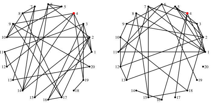
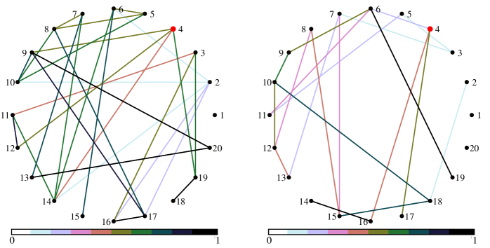
Figure 1: Original graphs: $\mathscr{G}_{1}$ (left) and $\mathscr{G}_{2}$ (right)

Figure 2: The optimal additional weights: $\Delta_{1}^{\star}$ (left) and $\Delta_{2}^{\star}$ (right)

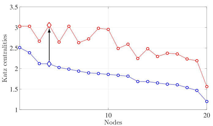
Figure 3: Katz centralities: Blue: before optimization. Red: after optimization. Diamonds indicate the target node $i=4$.

V Numerical Simulations

We illustrate the results obtained in this paper with numerical simulations. Let $\mathscr{G}_{1}$ and $\mathscr{G}_{2}$ be two independent realizations of Erdös-Rényi graphs with $n=20$ nodes and edge probability $p=0.15$ (shown in Fig. 2). We assume that the weights of the edges in both the graphs are all one. We consider the Markovian temporal network $\mathscr{G}$ taking values in the set $\{\mathscr{G}_{1},\mathscr{G}_{2}\}$ and having the transition probability matrix

$$P=\begin{bmatrix}0.5419&0.4581\\ 0.1914&0.8086\end{bmatrix}.$$

We fix $\alpha=0.1321=1/(2\rho(\mathscr{A}))$ and $\zeta_{0}=\mathbbold{1}_{2}/2$. We sort the nodes in $\mathscr{G}$ in the decreasing order of its Katz centrality.

For all $\ell\in\{1,2\}$ and $\{i,j\}\in\mathscr{E}_{\ell}$, we use the increasing cost function $f_{\ell,ij}(\Delta_{\ell,ij})=2(1-(\Delta_{ell,ij}+1)^{-1})$ defined over $[0,1]$. Let $\bar{\Delta}_{\ell}=A_{\ell}$ and $\underaccent{\bar}{A}_{\ell}=A_{\ell}$ for all $\ell$. Notice that the function $-f_{\ell,ij}$ is a posynomial in $\Delta_{\ell,ij}+1=\Delta_{\ell,ij}+\bar{A}_{\ell,ij}$ and therefore satisfies the assumption of Theorem IV.3. We let $i$ be the 4th important node, in terms of the Katz centrality of the original temporal network $\mathscr{G}$. We apply Algorithm 1 and obtain the optimal additional weights $\Delta_{1}^{\star}$ and $\Delta_{2}^{\star}$ with the cost $C=31.2$. We show the weighted graphs having the adjacency matrices $\Delta_{1}$ and $\Delta_{2}$ in Fig. 2. The Katz centralities of the original and optimized temporal networks are shown in Fig. 3.

For another but a larger-scale example, we again consider the Markovian temporal network whose layers are realizations of the Erdös-Rényi graphs. Here we choose the parameters $n=50$, $p=0.05$, and

$$P=\begin{bmatrix}0.1503&0.8497\\ 0.4381&0.5619\end{bmatrix}.$$

We fix $\alpha=0.1908=1/(2\rho(\mathscr{A}))$ and $\zeta_{0}=\mathbbold{1}_{2}/2$. We again sort the nodes in $\mathscr{G}$ in the decreasing order of its Katz centrality. We set the target node to be $i=8$, and use Algorithm 1 to obtain the optimal additional weights $\Delta_{1}^{\star}$ and $\Delta_{2}^{\star}$ (illustrated in Fig. 4) with the cost $C=43.05$. The Katz centralities of the original and optimized temporal networks are shown in Fig. 5.

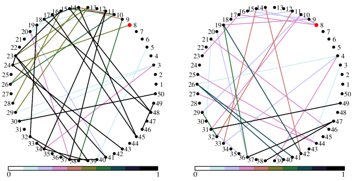
Figure 4: The optimal additional weights: $\Delta_{1}^{\star}$ (left) and $\Delta_{2}^{\star}$ (right)

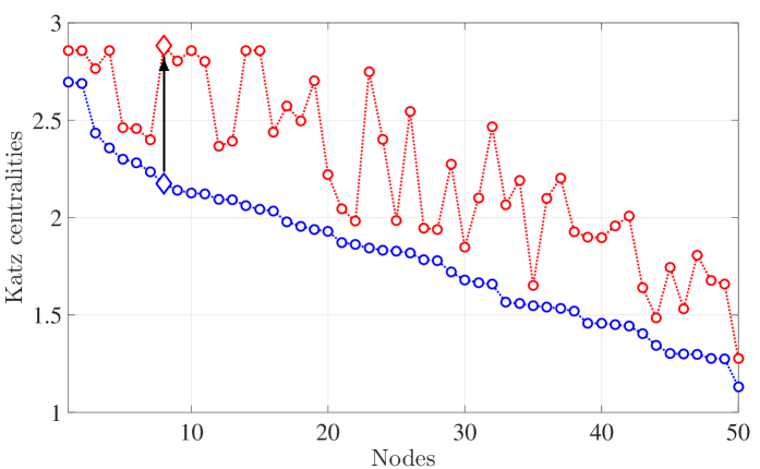
Figure 5: Katz centralities: Blue: before optimization. Red: after optimization. Diamonds indicate the target node $i=8$.

VI Conclusion

In this paper, we have introduced an extension of Katz centrality for Markovian temporal networks. The definition is based on the solution of a Markov jump linear system, which is consistent with the standard definition of Katz centrality for static networks. We have first shown that the Katz centrality of a Markovian temporal network is the solution of a linear program, which enables us to efficiently find the centrality in the case of large network sizes. We have then presented a convex optimization-based approach for controlling the Katz centrality by tuning the weights of the temporal network in the most cost-efficient manner. Numerical simulations have been given to illustrate the effectiveness of the obtained results.

References

- [1] P. V. Marsden, “Egocentric and sociocentric measures of network centrality,” Social Networks, vol. 24, pp. 407–422, 2002.
- [2] O. Hinz, B. Skiera, C. Barrot, and J. U. Becker, “Seeding strategies for viral marketing: an empirical comparison,” Journal of Marketing, vol. 75, pp. 55–71, 2011.
- [3] M. Girvan, and M. E. J. Newman, “Community structure in social and biological networks,” Proceedings of the National Academy of Sciences of the United States of America, vol. 99, pp. 7821–7826, 2002.
- [4] D. F. Gleich, “PageRank beyond the Web,” SIAM Review, vol. 57, pp. 321–363, 2014.
- [5] L. Page, S. Brin, R. Motwani, and T. Winograd, “The PageRank citation ranking: bringing order to the web,” Stanford University, Tech. Rep., 1998.
- [6] P. Bonacich, “Power and centrality: a family of measures,” American Journal of Sociology, vol. 92, pp. 1170–1182, 1987.
- [7] L. Katz, “A new status index derived from sociometric analysis,” Psychometrika, vol. 18, pp. 39–43, 1953.
- [8] J. Kleinberg, “Authoritative sources in a hyperlinked environment,” Journal of the ACM, vol. 46, no. 5, pp. 604–632, 1999.
- [9] P. Holme, “Modern temporal network theory: a colloquium,” The European Physical Journal B, vol. 88, p. 234, 2015.
- [10] D. Braha and Y. Bar-Yam, “From centrality to temporary fame: Dynamic centrality in complex networks,” Complexity, vol. 12, pp. 59–63, 2006.
- [11] K. Lerman, R. Ghosh, and J. H. Kang, “Centrality metric for dynamic networks,” Information Sciences, vol. 354, pp. 70–77, 2010.
- [12] J. Tang, M. Musolesi, C. Mascolo, V. Latora, and V. Nicosia, “Analysing information flows and key mediators through temporal centrality metrics categories and subject descriptors,” in 3rd Workshop on Social Network Systems, 2010.
- [13] P. Grindrod and D. J. Higham, “A dynamical systems view of network centrality,” Proceedings of the Royal Society A: Mathematical, Physical and Engineering Sciences, vol. 470:201308, 2014.
- [14] R. A. Rossi and D. F. Gleich, “Dynamic PageRank using evolving teleportation,” in Algorithms and Models for the Web Graph, 2012, pp. 126–137.
- [15] O. Fercoq, M. Akian, M. Bouhtou, and S. Gaubert, “Ergodic control and polyhedral approaches to pagerank optimization,” IEEE Transactions on Automatic Control, vol. 58, pp. 134–148, 2013.
- [16] B. C. Csáji, R. M. Jungers, and V. D. Blondel, “PageRank optimization by edge selection,” Discrete Applied Mathematics, vol. 169, pp. 73–87, 2014.
- [17] A. R. Masson, E. Altman, and Y. Hayel, “Controlling the Katz-Bonacich centrality in social network: application to gossip in online social networks,” in 2015 IEEE/ACM 8th International Conference on Utility and Cloud Computing, 2015, pp. 442–447.
- [18] R. Horn and C. Johnson, Matrix Analysis. Cambridge University Press, 1990.
- [19] S. Boyd, S.-J. Kim, L. Vandenberghe, and A. Hassibi, “A tutorial on geometric programming,” Optimization and Engineering, vol. 8, pp. 67–127, 2007.
- [20] E. Volz and L. A. Meyers, “Epidemic thresholds in dynamic contact networks.” Journal of the Royal Society, Interface / the Royal Society, vol. 6, pp. 233–241, 2009.
- [21] N. Perra, B. Gonçalves, R. Pastor-Satorras, and A. Vespignani, “Activity driven modeling of time varying networks.” Scientific Reports, vol. 2:469, 2012.
- [22] M. Ogura and V. M. Preciado, “Stability of spreading processes over time-varying large-scale networks,” IEEE Transactions on Network Science and Engineering, vol. 3, pp. 44–57, 2016.
- [23] ——, “Optimal design of switched networks of positive linear systems via geometric programming,” IEEE Transactions on Control of Network Systems (accepted), 2015.
- [24] M. Ogura and C. F. Martin, “Stability analysis of positive semi-Markovian jump linear systems with state resets,” SIAM Journal on Control and Optimization, vol. 52, pp. 1809–1831, 2014.
- [25] L. Farina and S. Rinaldi, Positive Linear Systems: Theory and Applications. Wiley-Interscience, 2000.