Conformalized Kernel Ridge Regression

Abstract

General predictive models do not provide a measure of confidence in predictions without Bayesian assumptions. A way to circumvent potential restrictions is to use conformal methods for constructing non-parametric confidence regions, that offer guarantees regarding validity. In this paper we provide a detailed description of a computationally efficient conformal procedure for Kernel Ridge Regression (KRR), and conduct a comparative numerical study to see how well conformal regions perform against the Bayesian confidence sets. The results suggest that conformalized KRR can yield predictive confidence regions with specified coverage rate, which is essential in constructing anomaly detection systems based on predictive models.
Keywords: kernel ridge regression, gaussian process regression, conformal prediction, confidence region.

I Introduction

In many applied situations, like anomaly detection in telemetry of some equipment, online filtering and monitoring of potentially interesting events, or power grid load balancing, it is necessary not only to make optimal predictions with respect to some loss, but also to be able to quantify the degree of confidence in the obtained forecasts. At the same time it is necessary to take into consideration exogenous variables, that in certain ways affect the object of study.

Practical importance and difficulty of anomaly detection in general spurred a great deal of research, which resulted in a large volume of heterogeneous approaches and methods to its solution ([1, 2, 3]). There are many approaches: probabilistic, which rely on approximating the generative distribution of the observed data ([4, 5]), metric-based anomaly detection, that measure similarity between normal and abnormal observations ([6, 7, 8]), predictive modelling approaches, which use the forecast error to measure abnormality ([9, 10, 11, 12]).

Predictive modelling is concerned with recovering an unobserved relation $x\mapsto f(x)$ from a sample $(x_{i},y_{i})_{i=1}^{n}$ of noisy observations

$$y_{i}=f(x_{i})+\epsilon_{i}\,,$$ (1)

where $\epsilon_{i}$ is iid with mean zero. One way of assigning a confidence measure to a prediction $\hat{f}$ is by using assumptions on the geometric structure of the manifold approximating the sample data which provide estimates of the likelihood of the prediction error for the test data, [13, 14]. Another approach is to quantify estimate’s, model’s and observational uncertainty, by imposing Bayesian assumptions (eq. 1).

Consider Kernel Ridge Regression – a model that combines ridge regression with the kernel trick. It learns a function $\hat{f}$ which, given training sample $X=(x_{i})_{i=1}^{n}$, $X\in\mathcal{X}^{n\times 1}$, solves

$$\|y-f(X)\|^{2}+\lambda\|f\|^{2}\to\min_{f\in\mathcal{H}}\,,$$

with $f(X)=(f(x_{i}))_{i=1}^{n}\in\mathbb{R}^{n\times 1}$, and $y=(y_{i})_{i=1}^{n}\in\mathbb{R}^{n\times 1}$. Here $\mathcal{H}$ is the canonical Reproducing Kernel Hilbert Space associated with a Mercer-type kernel $\mathcal{K}:\mathcal{X}\times\mathcal{X}\mapsto\mathbb{R}$. The Representer theorem, [15], states that the solution $\hat{f}:\mathcal{X}\mapsto\mathbb{R}$ is of the form $f(x)=k_{x}^{\prime}\beta$, for $k_{x}:x\mapsto\Phi(x)$ and $\Phi=(\phi(x_{i}))_{i=1}^{n}\in\mathcal{H}^{n\times 1}$. If $e_{j}$ is the $j$-th unit vector in $\mathbb{R}^{n\times 1}$, and $K_{XX}$ is the Gram matrix of $\mathcal{K}$ over $(x_{i})_{i=1}^{n}$, then $f(x_{j})=k_{x_{j}}^{\prime}\beta=e_{j}^{\prime}K_{XX}\beta$ and $\|f\|^{2}=\beta^{\prime}K_{XX}\beta$. Thus the kernel ridge regression problem is equivalent to this finite-dimensional convex minimization problem:

$$\|y-K_{XX}\beta\|^{2}+\lambda\beta^{\prime}K_{XX}\beta\to\min_{\beta\in\mathbb{R}^{n\times 1}}\,,$$

which yields the optimal weight vector $\hat{\beta}$ and prediction at $x^{*}\in\mathcal{X}$ given by $\hat{\beta}=(\lambda I_{n}+K_{XX})^{-1}y$ and $\hat{y}(x^{*})=k_{x^{*}}^{\prime}\hat{\beta}$, respectively.

Bayesian Kernel Ridge Regression views the model eq. 1 as a sample path of the underlying Gaussian Process, [16], which makes predictive confidence intervals readily available. A Gaussian Process $(y_{x})_{x\in\mathcal{X}}$, with mean $m:\mathcal{X}\mapsto\mathbb{R}$ and covariance kernel $\mathcal{K}:\mathcal{X}\times\mathcal{X}\mapsto\mathbb{R}$ is a random process such that for any $n\geq 1$ and any $X=(x_{i})_{i=1}^{n}\in\mathcal{X}$ the $n\times 1$ vector $y_{X}=(y(x_{i}))_{i=1}^{n}$ is Gaussian, $y_{X}\sim\mathcal{N}_{n}(m_{X},K_{XX})$, where $m_{X}=(m(x_{i}))_{i=1}^{n}$. The conditional distribution of targets in a test sample $y_{X^{*}}=(y_{x^{*}_{j}})_{j=1}^{l}$ with respect to the train sample $y_{X}=(y_{x_{i}})_{i=1}^{n}$ is given by

$$y_{X^{*}}|_{y_{X}}\sim\mathcal{N}_{l}\bigl{(}m_{X^{*}}+K_{X^{*}X}Q_{X}(y_{X}-m_{X}),\Sigma_{K}(X^{*})\bigr{)}\,,$$ (2)

where $\Sigma_{K}(X^{*})=K_{X^{*}X^{*}}-K_{X^{*}X}Q_{X}K_{XX^{*}}$, $Q_{X}=\bigl{(}K_{XX}\bigr{)}^{-1}$, and $K_{XX^{*}}=(\mathcal{K}(x_{i},x^{*}_{j}))\in\mathbb{R}^{n\times l}$. Gaussian Process Regression, or Kriging, generalizes both linear and kernel regression and assumes linearity of the mean function with respect to $x$ and external factors $h$.

Bayesian KRR assumes a prior on functions $f\sim GP(0,\sigma^{2}\mathcal{K})$ and independent Gaussian white noise $\epsilon_{x}\sim\mathcal{N}(0,\sigma^{2}\lambda)$ in model 1, for $\sigma^{2}>0$. In this setting, eq. 2 implies that the distribution of a yet unobserved target $y_{x^{*}}$ at $x^{*}\in\mathcal{X}$, conditional on the train data $(X,y_{X})$, is

$${y_{x^{*}}}_{|y_{X}}\sim\mathcal{N}\bigl{(}\hat{y}_{y_{X}}(x^{*}),\sigma^{2}\sigma_{K}^{2}(x^{*})\bigr{)}\,,$$ (3)

with $\hat{y}_{y_{X}}(x^{*})=K_{X}(x^{*})^{\prime}Q_{X}y_{X}$, and

$$\sigma_{K}^{2}(x^{*})=\lambda+K(x^{*},x^{*})-K_{X}(x^{*})^{\prime}Q_{X}K_{X}(x^{*})\,,$$

where $Q_{X}=\bigl{(}\lambda I_{n}+K_{XX}\bigr{)}^{-1}$, $K_{XX}=(K(x_{i},x_{j}))_{ij}$, and $K_{X}=(K(x_{i},\cdot))_{i=1}^{n}:\mathcal{X}\mapsto\mathbb{R}^{n\times 1}$. Thus, the $1-\alpha$ confidence interval is thus given by

$$\Gamma^{\alpha}_{y_{X}}(x^{*})=\hat{y}_{y_{X}}(x^{*})+\sigma\sqrt{\sigma_{K}^{2}(x^{*})}\times[z_{\frac{\alpha}{2}},z_{1-\frac{\alpha}{2}}]\,,$$ (4)

where $z_{\gamma}$ is the $\gamma$ quantile of $\mathcal{N}(0,1)$. Additionally, this version naturally permits estimation of parameters of the underlying kernel $\mathcal{K}$ through maximization of the joint likelihood of the train data $(X,y_{X})$:

$$\mathcal{L}=-\frac{n}{2}\log 2\pi-\frac{n}{2}\log\sigma^{2}-\frac{1}{2}\log\lvert R_{X}\rvert-\frac{1}{2\sigma^{2}}y^{\prime}R_{X}^{-1}y\,,$$ (5)

where $R_{X}=\lambda I_{n}+K_{XX}$, and $K_{XX}$ depends on the hyper-parameters of $\mathcal{K}$ (shape, precision et c.). Other approaches to estimating the covariance function’s hyper-parameters are reported in [17], properties of posterior parameter distribution in Bayesian KRR are studied in [18], methods of estimating Gaussian Process Regression on large structured datasets are considered in [19, 20], and the problem of estimating in non-stationary case with regularization is considered in [21].

It is desirable to have distribution-free method that measures confidence of predictions of a machine learning algorithm. One such method is ‘‘Conformal prediction’’ – an approach developed in [22], which under standard independence assumptions yields a set in the space of targets, that contains yet unobserved data with a pre-specified probability. In this study, we provide empirical evidence supporting the claim that when model assumptions do hold, the conformal confidence sets, constructed over the Kernel Ridge Regression with isotropic Gaussian kernel do not perform worse than the prediction confidence intervals of a Bayesian version of the KRR. The paper is structured as follows: in section II a concise overview of what conformal prediction is and what is required to construct such kind of confidence predictor is given. Section III describes the particular steps needed to build a conformal predictor atop the kernel ridge regression. The main empirical study is reported in section IV, where we study the properties of the predictor in a batch learning setting for a KRR with specific kernel.

II Conformal prediction

Conformal prediction is a distribution-free technique designed to yield a statistically valid confidence sets for predictions made by machine learning algorithms. The key advantage of the method is that it offers coverage probability guarantees under standard IID assumptions, even in cases when assumptions of the underlying prediction algorithm fail to be satisfied. The method was introduced in [22] for online supervised and unsupervised learning.

Let $\mathcal{Z}$ denote the object-target space $\mathcal{X}\times\mathcal{Y}$. At the core of a conformal predictor is a measurable map $A:\mathcal{Z}^{*}\times\mathcal{Z}\mapsto\mathbb{R}$, a Non-Conformity Measure (NCM), which quantifies how much different $z_{n+1}\in\mathcal{Z}$ is relative to a sample $Z_{:n}=(z_{i})_{i=1}^{n}\in\mathcal{Z}$. A conformal predictor over $A$ is a procedure, which for every sample $Z_{:n}$, a test object $x_{n+1}\in\mathcal{X}$, and a level $\alpha\in(0,1)$, gives a confidence set $\Gamma_{Z_{:n}}^{\alpha}(x^{*})$ for the target value $y_{n+1}$:

$$\Gamma_{Z_{:n}}^{\alpha}(x_{n+1})=\bigl{\{}y\in\mathcal{Y}\,:\,p_{Z_{:n}}(\tilde{z}^{y}_{n+1})\geq\alpha\bigr{\}}\,,$$ (6)

where $\tilde{z}^{y}_{n+1}=(x_{n+1},y)$ a synthetic test observation with target label $y$. The function $p:\mathcal{Z}^{*}\times(\mathcal{X}\times\mathcal{Y})\mapsto[0,1]$ measures the likelihood of $\tilde{z}$ based on its non-conformity with $Z_{:n}$, and is

$$p_{Z_{:n}}(\tilde{z})=(n+1)^{-1}\bigl{\lvert}\{i\,:\,\eta_{i}^{\tilde{z}}\geq\eta_{n+1}^{\tilde{z}}\}\bigr{\rvert}\,,$$ (7)

where $i=1,\ldots,n+1$, and $\eta_{i}^{\tilde{z}}=A(S^{\tilde{z}}_{-i},S^{\tilde{z}}_{i})$ – the non-conformity of the $i$-th observation with respect to the augmented sample $S^{\tilde{z}}=(Z_{:n},{\tilde{z}}^{y}_{n+1})\in\mathcal{Z}^{n+1}$. For any $i$, $S^{\tilde{z}}_{i}$ is the $i$-th element of the sample, and $S^{\tilde{z}}_{-i}$ is the sample with the $i$-th observation omitted.

For every possible value $z$ of an object $Z_{n+1}$ the conformal procedure tests $H_{0}:Z_{n+1}=z$, and then inverts the test to get a confidence region. The hypothesis tests are designed to have a fixed empirical type-I error rate $\alpha$ based on the observed sample $Z_{:n}$ and hypothesized $z$.

In [22], chapter 2, is has been shown, that for sequences of iid examples $(z_{n})_{n\geq 1}\sim P$, the coverage probability of the prediction set $\Gamma^{\alpha}$, 6, is at least $1-\alpha$ and successive errors are independent in online learning and prediction setting. The procedure guarantees unconditional validity: for any $\alpha\in(0,1)$

$$\mathop{\mathbb{P}}\nolimits_{Z_{:n}\sim P}\bigl{(}y_{n}\notin\Gamma^{\alpha}_{Z_{:(n-1)}}(x_{n})\bigr{)}\leq\alpha\,,$$ (8)

where $(x_{n},y_{n})=z_{n}$. Intuitively, the event $y_{n}\notin\Gamma^{\alpha}_{Z_{:(n-1)}}(x_{n})$ is equivalent to $\eta_{n}=A(Z_{-n},Z_{n})$ being among the largest $\lfloor n\alpha\rfloor$ values of $\eta_{i}=A(Z_{-i},Z_{i})$, which is equal to $\frac{\lfloor n\alpha\rfloor}{n}$, due to independence of $Z_{:n}$ (for a rigorous proof see [22], ch. 8).

The choice of NCM affects the size of the confidence sets and the computational burden of the conformal procedure. In the general case computing eq. 6 requires exhaustive search through the target space $\mathcal{Y}$, which is infeasible in general regression setting. However, for specific non-conformity measures it is possible to come up with efficient procedures for computing the confidence region as demonstrated in [22] and sec. III of this work.

III Conformalized kernel ridge regression

In this section we describe the construction of confidence regions of the conformal procedure eq. 6 for the case of the non-conformity measures based on kernel ridge regression. We consider two NCMs defined in terms of regression residuals: the one used in constructing a ‘‘Ridge Regression Confidence Machine’’, proposed in [22], chapter 2, and ‘‘two-sided’’ NCM, proposed in [23].

III-A Residuals

In each NCM it is possible to use any kind of prediction error, but we focus on two: the in-sample and leave-one-out (or deleted) residuals. Consider a sample $(X,y)=(x_{i},y_{x_{i}})_{i=1}^{n}$, and for any $i=1\ldots,n$ put $X=(X_{-i},x_{i})$, and $y=(y_{-i},y_{i})$. In-sample residuals, $\hat{r}_{\text{in}}(X,y)$, are defined for each $i$ as

$$e_{i}^{\prime}\hat{r}_{\text{in}}(X,y)=y_{i}-\hat{y}_{|(X,y)}(x_{i})\,,$$ (9)

and LOO $\hat{r}_{\text{loo}}(X,y)$ are given by

$$e_{i}^{\prime}\hat{r}_{\text{loo}}(X,y)=y_{i}-\hat{y}_{|(X_{-i},y_{-i})}(x_{i})\,,$$ (10)

where $\hat{y}_{|(X,y)}$ and $\hat{y}_{|(X_{-i},y_{-i})}$ denote predictions of a KRR fit on the whole sample $(X,y)$, and a sample $(X_{-i},y_{-i})$ with the $i$-th observation knocked-out, respectively. For any $i$ the residuals are related by

$$e_{i}^{\prime}\hat{r}_{\text{in}}(X,y)=\lambda m_{i}^{-1}e_{i}^{\prime}\hat{r}_{\text{loo}}(X,y)\,,$$ (11)

where $\lambda m_{i}^{-1}=\lambda e_{i}^{\prime}Q_{X}e_{i}$ is the KRR ‘‘leverage’’ score of the $i$-th observation, and

$$m_{i}=\lambda+\mathcal{K}(x_{i},x_{i})-k_{-i}(x_{i})^{\prime}Q_{-i}k_{-i}(x_{i})\,,$$ (12)

with $k_{-i}(x_{i})$ – the $n-1\times 1$ vector of $(\mathcal{K}(x_{j},x_{i}))_{i\neq j}$, $Q_{-i}=(K_{-i}+\lambda I_{n-1})^{-1}$, and $K_{-i}$ is the Gram matrix of the kernel $\mathcal{K}$ over subsample $X_{-i}$.

III-B Ridge Regression Confidence Machine

In this section we describe a conformal procedure for the NMC proposed in [22], chapter 2, and focus on its ‘‘in-sample’’ version, bearing in mind that residuals (10) and (9) are interchangeable.

The Ridge Regression Confidence Machine (RRCM) constructs an non-conformity measure from the absolute value of the regression residual: the ‘‘in-sample’’ NCM, $A_{\text{in}}$, is given by

$$A_{\text{in}}\bigl{(}(X_{-i},y_{-i}),(x_{i},y_{i})\bigr{)}=|e_{i}^{\prime}\hat{r}_{\text{in}}(X,y)|\,,$$ (13)

and the ‘‘LOO’’ NCM, $A_{\text{loo}}$ is defined similarly using eq. 10. For the NCM $A$ the $1-\alpha$ conformal confidence interval for the $n$-th observation is given by

$$\Gamma_{X_{-n},y_{-n}}^{\alpha}(x_{n})=\bigl{\{}z\in\mathbb{R}\,:\,p_{n}\bigl{(}(X,\tilde{y}_{n}^{z})\bigr{)}\geq\alpha\bigr{\}}\,,$$ (14)

where $\tilde{y}_{i}^{z}=(y_{-i},z)$ – the augmented target sample $y$ with the $i$-th value replaced by $z$. The ‘‘conformal likelihood’’ of the $i$-th observation in some sample $(X,y)$ is given by

$$p_{j}\bigl{(}(X,y)\bigr{)}=n^{-1}\bigl{\lvert}\bigl{\{}j=1,\ldots,n\,:\,\eta_{j}\geq\eta_{i}\bigr{\}}\bigr{\rvert}\,,$$

for $\eta_{i}=A\bigl{(}(X_{-i},y_{-i}),(x_{i},y_{i})\bigr{)}$.

Efficient construction of the confidence set for the NCM (13) for in-sample (and deleted) residuals relies on linear dependence on the target of the $n$-th observation:

$$\hat{r}_{i}^{z}=e_{i}^{\prime}\hat{r}_{\text{in}}(X,\tilde{y}_{n}^{z})=\lambda c_{i}+\lambda b_{i}z\,,$$ (15)

with $c_{i}=e_{i}^{\prime}C_{-n}\bigl{(}(X,y),x_{n}\bigr{)}$ and $C_{-n}\bigl{(}(X,y),x_{n}\bigr{)}$ given by

$$\begin{pmatrix}Q_{-n}y_{-n}\\ 0\end{pmatrix}-B_{-n}(x_{n})K_{-n}(x_{n})^{\prime}Q_{-n}y_{-n}\,,$$

where $0$ is scalar and the vector $B_{-n}(x_{n})\in\mathbb{R}^{n\times 1}$ is

$$B_{-n}(x_{n})=\begin{pmatrix}-Q_{-n}K_{-n}(x_{n})\\ 1\end{pmatrix}m_{n}^{-1}\,.$$ (16)

Since absolute values of the residuals are compared, it is possible to consistently change the signs of each element of $C$ and $B$ to ensure that $e_{i}^{\prime}B\geq 0$ for all $i$.

The conformal p-value for $(x_{n},y)$, eq. , is can be re-defined in terms of regions $S_{i}=\{z\in\mathbb{R}\,:\,|\hat{r}_{i}^{z}|\geq|\hat{r}_{n}^{z}|\}$, for $i=1,\ldots,n$:

$$p_{X_{-n},y_{-n}}(x_{n},y)=n^{-1}\bigl{\lvert}\{i\,:\,y\in S_{i}\}\bigr{\rvert}\,.$$ (17)

These regions are either closed intervals, complements of open intervals, one-side closed half-rays in $\mathbb{R}$, depending on the values of $C$ and $B$. In particular, with $p_{i}$ and $q_{i}$ denoting $-\frac{c_{i}+c_{n}}{b_{i}+b_{n}}$ and $\frac{c_{i}-c_{n}}{b_{n}-b_{i}}$, respectively (whenever each is defined), each region $S_{i}$ has one of the following representations:

1. $b_{i}=b_{n}=0$: $S_{i}=\mathbb{R}$ if $|c_{i}|\geq|c_{n}|$, or $S_{i}=\emptyset$ otherwise;

2. $b_{n}=b_{i}>0$: $S_{i}$ is either $(-\infty,p_{i}]$ if $c_{i}<c_{n}$, $[p_{i},+\infty)$ if $c_{i}>c_{n}$, or $\mathbb{R}$ otherwise;

3. $b_{n}>b_{i}\geq 0$: $S_{i}$ is either $[p_{i},q_{i}]$ if $c_{i}b_{n}\geq c_{n}b_{i}$, or $[q_{i},p_{i}]$ otherwise;

4. $b_{i}>b_{n}\geq 0$: $S_{i}$ is $\mathbb{R}\setminus(q_{i},p_{i})$ when $c_{i}b_{n}\geq c_{n}b_{i}$, or $\mathbb{R}\setminus(p_{i},q_{i})$ otherwise.

Let $P$ and $Q$ be the sets of all well-defined $p_{i}$ and $q_{i}$ respectively, and let $(g_{j})_{j=0}^{J+1}$ enumerate distinct values of $\{\pm\infty\}\cup P\cup Q$, so that $g_{j}<g_{j+1}$ for all $j$. Then the confidence region is a closed subset of $\mathbb{R}$ constructed from sets $G^{m}_{j}=[g_{j},g_{j+m}]\cap\mathbb{R}$ for $m=0,1$:

$$\Gamma_{X_{-n},y_{-n}}^{\alpha}(x_{n})=\bigcup_{m\in\{0,1\}}\bigcup_{j\,:\,N^{m}_{j}\geq n\alpha}G^{m}_{j}\,,$$ (18)

where $N^{m}_{j}=|\{i\,:\,G^{m}_{j}\subseteq S_{i}\}|$ is the coverage frequency of $G^{m}_{j}$, eq. 17. In general, the resulting confidence set might contain isolated singletons $G^{0}_{j}$.

This set, can be constructed efficiently in $\mathcal{O}(n\log{}n)$ time with $\mathcal{O}(n)$ memory footprint. Indeed, it is necessary to sort at most $J\leq 2n$ distinct endpoints of $G_{j}$, then locate the values $p_{i}$ and $q_{i}$ associated with each region $S_{i}$ ($\mathcal{O}(n\log{}n)$). Then, since the building blocks $G^{m}_{j}$ of $\Gamma^{\alpha}$ are either singletons ($m=0$), or intervals made up from adjacent singletons ($m=1$), coverage numbers $N^{m}_{j}$ can be computed in at most $\mathcal{O}(n)$ time.

III-C Kernel two-sided confidence predictor

Another possibility is to use the two-sided conformal procedure, proposed in [23]. The main result of that paper is that under relaxed Bayesian Ridge Regression assumptions if a sequence $(x_{n})_{n\geq 1}\in\mathcal{X}$ is i.i.d. with an non-singular second moment matrix $\mathop{\mathbb{E}}\nolimits x_{1}x_{1}^{\prime}\succeq 0$, then for all sufficiently large $n$ the conformal confidence regions that lose little efficiency (the upper endpoints of the Bayesian and conformal prediction intervals deviate as much as $\mathcal{O}_{p}\bigl{(}n^{-\frac{1}{2}}\bigr{)}$).

The ‘‘two-sided’’ procedure of [23], denoted by CRR for short, uses a conformity measure

$$A(Z_{-i},Z_{i})=\bigl{\lvert}\{j\,:\,\hat{r}_{j}\geq\hat{r}_{i}\}\bigr{\rvert}\wedge\bigl{\lvert}\{j\,:\,\hat{r}_{j}\leq\hat{r}_{i}\}\bigr{\rvert}\,,$$ (19)

where $(\hat{r}_{i})_{i=1}^{n}$ are the in-sample ridge regression residuals. In that paper it was also shown that for any $\alpha\in(0,1)$ the confidence region $\Gamma^{\alpha}$ produced by CRR procedure for the conformity measure in eq. 19 is equivalent to the intersection of confidence sets yielded by conformal procedures with non-conformity measures given by $\eta_{i}=\hat{r}_{i}$ and $\eta_{i}=-\hat{r}_{i}$ at significance levels $\frac{\alpha}{2}$. Individually, these NCMs define a upper and lower CRR sets respectively, and together constitute a ‘‘two-sided’’ conformal procedure. Confidence regions based on this NCM, much like RRCM, can use any kind of residual: leave-one-out, or in-sample.

For the upper CRR the regions $U_{i}=\{z\in\mathbb{R}\,:\,\hat{r}_{i}^{z}\geq\hat{r}_{n}^{z}\}$, $i=1,\ldots,n$, are either empty, full $\mathbb{R}$ or one-side closed half-rays. Since $\hat{r}_{i}^{z}=\lambda c_{i}+\lambda b_{i}z$, $U_{i}$ takes one of the following forms:

1. $b_{i}=b_{n}$: $U_{i}=\mathbb{R}$ if $c_{i}\geq c_{n}$, and $\emptyset$ otherwise;

2. $b_{i}\neq b_{n}$: $U_{i}=[q_{i},+\infty)$ if $b_{i}>b_{n}$, or $U_{i}=(-\infty,q_{i}]$ otherwise;

with $q_{i}=\frac{c_{i}-c_{n}}{b_{n}-b_{i}}$. The forms of regions $L_{i}$ for the lower CRR are computed similarly, but with the signs of $c_{i}$ and $b_{i}$ flipped for each $i=1,\ldots,n$.

Both upper and lower confidence regions are built similarly to the kernel RRCM region eq. 18 in sec. III-B. The final Kernel CRR confidence set is given by

$$\Gamma_{X_{-n},y_{-n}}^{\alpha}(x_{n})=\Gamma_{X_{-n},y_{-n}}^{\alpha,\text{u}}(x_{n})\cap\Gamma_{X_{-n},y_{-n}}^{\alpha,\text{l}}(x_{n})\,.$$ (20)

This intersection can be computed efficiently in $\mathcal{O}(n\log{}n)$, since the regions are built form sets anchored at a finite set $Q$ with at most $n+2$ values. Therefore, the CRR confidence set for a fixed significance level $\alpha$ has $\mathcal{O}(n\log{}n)$ complexity.

IV Numerical study

Validity of conformal predictors in the online learning setting has been shown in [22], chapter 2, however, no result of this kind is known in the batch learning setting. Our experiments aim to evaluate the empirical performance of the conformal prediction in this setting: with dedicated train and test datasets. In this section we conduct a set of experiments to examine the validity of the regions, produced by the conformal Kernel Ridge Regression and compare its efficiency to the Bayesian confidence intervals. We use the isotropic Gaussian kernel with the precision parameter $\theta>0$, $\mathcal{K}(x,x^{\prime})=\mathop{\text{exp}}\bigl{\{}-\theta\|x-x^{\prime}\|^{2}\bigr{\}}$, for both the Conformal Kernel ridge regression and the Gaussian Process Regression. We experiment on a compact set $\mathcal{X}\subset\mathbb{R}^{d\times 1}$, since the validity of conformal region is by design unaffected by the NCM $A$, which can be an arbitrary computable function and is oblivious to the structure of the domain. The dimensionality of the input data, however, may impact the width of the constructed confidence region.

The off-line validity and efficiency of Bayesian and Conformal confidence regions is studied in two settings: the fully Gaussian case, and the non-Gaussian cases. In the first case the Bayesian assumptions hold and experiments are run on a sample path of $GP(0,\mathcal{K}+\delta_{x,x^{\prime}}\gamma)$. In the second the assumptions of Gaussian Process Regression are partially valid: a deliberately non-Gaussian $f$ in eq. 1 is contaminated by moderate Gaussian white noise with variance $\gamma$.

The following hyper-parameters are controlled: the true noise-to-signal ratio $\gamma\in\{10^{-6},10^{-1}\}$, the covariance kernel precision $\theta\in\{10,10^{2},10^{3}\}$, the train sample size $n$ (from $25$ up to $1600$), the NCM (eq. 13 RRCM, or eq. 19 CRR), the residual eq. 9, or eq. 10, the regularization parameter $\lambda\in\{10^{-1},10^{-6}\}$, and either fixed $\theta$ or $\theta$ that minimizes eq. 5.

For a given test function $f:\mathcal{X}\mapsto\mathbb{R}$ and a set of hyper-parameters each experiment consists of the following steps:

1. The test inputs, $X^{*}$, are given by a regular grid in $\mathcal{X}$ with constant spacing;

2. Train inputs, $X$, are sampled from a uniform distribution over $\mathcal{X}$;

3. For all $x\in X_{\text{pool}}=X\cup X^{*}$, target values $y_{x}=f(x)$ are generated;

4. For $l=1,\ldots,L$ independently

   1. draw a random subsample of size $n$ from train dataset;

   2. fit a Gaussian Process Regression with zero mean and Gaussian kernel $\mathcal{K}$ with the specified precision $\theta$ and $\lambda$;

   3. for each $x^{*}\in X^{*}$ construct the Bayesian (eq. 4) and conformal (eq. 6) confidence regions using the NCM $A$ and residuals $\hat{r}$ with MLE estimated $\sigma^{2}$;

   4. estimate the coverage rate and the width of the convex hull of the region over the test sample $X^{*}$: $p_{l}(R)=|X^{*}|^{-1}\sum_{x\in X^{*}}1_{y_{x}\in R_{x}}$, and $w_{l}(R)=\inf\{b-a\,:\,R\subseteq[a,b]\}$, where $R$ is a confidence region;

With the experimental procedure properly outlined, we proceed to summarizing the results.

IV-A Results: $1$-d

We begin with the examination of the fully-Gaussian setup with $\mathcal{X}=[0,1]$. To illustrate the constructed confidence regions, we generated a sample path of the $1$-d Gaussian process with isotropic Gaussian kernel on a regular grid of $501$ knots, and use a subset of $51$ knots in $[0.05,0.95]$ for constructing the Bayesian (GPR) and conformal (RRCM) confidence regions. The confidence regions are depicted in fig. 1: conformal regions closely track the Bayesian confidence bands (‘‘GPR-f’’, eq. 4), but the latter are too wide in the low noise case. Near the endpoints the confidence regions dramatically increase in width, reflecting increased uncertainty. In general, the conformal regions necessarily cover the KRR prediction $\hat{y}^{*}_{|(X,y)}(x^{*})$ but are not necessarily symmetric around it, where as GPR regions are (eq. 4).

In can be argued, that confidence regions for any observation $x_{n}$ sufficiently far away from the bulk of the training dataset have constant size, determined only by the train sample (fig. 2). Indeed, as $\|x_{n}\|^{2}\to\infty$ ($n$-fixed) the vector $B_{-n}$ in (eq. 16) approaches the $n$-th unit vector $e_{n}$, since for the Gaussian kernel the vector $\|K_{-n}(x_{n})\|^{2}\to 0$. Since the kernel is bounded, the value $m_{n}$ (eq. 12) is a bounded function of $x_{n}$, which, in turn, implies that eventually all RRCM (similarly, CRR) regions $S_{i}$ assume the form of closed intervals $[-|q_{i}|,|q_{i}|]$, where $q_{i}=m_{n}(e_{i}^{\prime}Q_{-n}y_{-n})+o(\|x_{n}\|^{2})$, $i\neq n$. Therefore, the conformal procedure essentially reverts to a constant-size confidence region, determined by the $n^{-1}\lfloor n(1-\alpha)\rfloor$-th order statistic of $(|q_{i}|)_{i=1}^{n}$. Analogous effects can be observed for the Gaussian Process confidence interval (eq. 4).

By construction, conformal confidence region (eq. 6) allows for some uncertainty. Indeed, the residuals (eq. 15) and hence the vector of non-conformity scores $(\eta^{z}_{i})_{i=1}^{n}$ are continuous functions of targets $y=(y_{i})_{i=1}^{n}$. Thus for small perturbations of $y$ the relative ordering of $\eta^{z}_{i}$ is kept, and the interval remains unchanged. Therefore, eq. 6 tends to capture more points $y$ for the same fixed significance level.

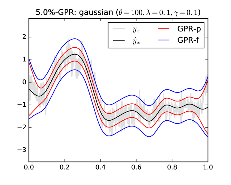
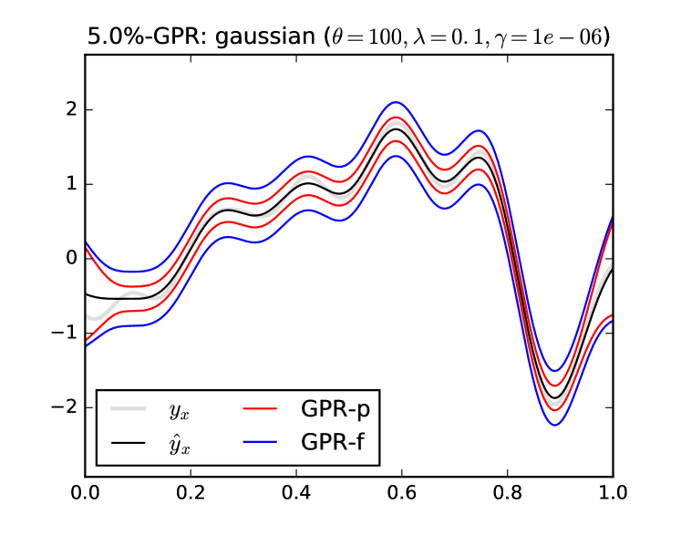
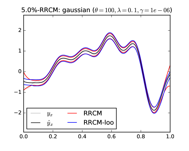
Figure 1: A sample path of a $1$-d Gaussian Process with $\gamma=10^{-1}$ (top), and $\gamma=10^{-6}$ (bottom) constructed confidence intervals: the forecast ‘‘GPR-f’’ and prediction ‘‘GPR-p’’ (left), and the ‘‘RRCM’’ confidence bands (right).

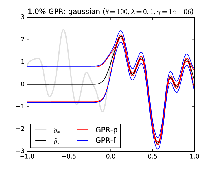
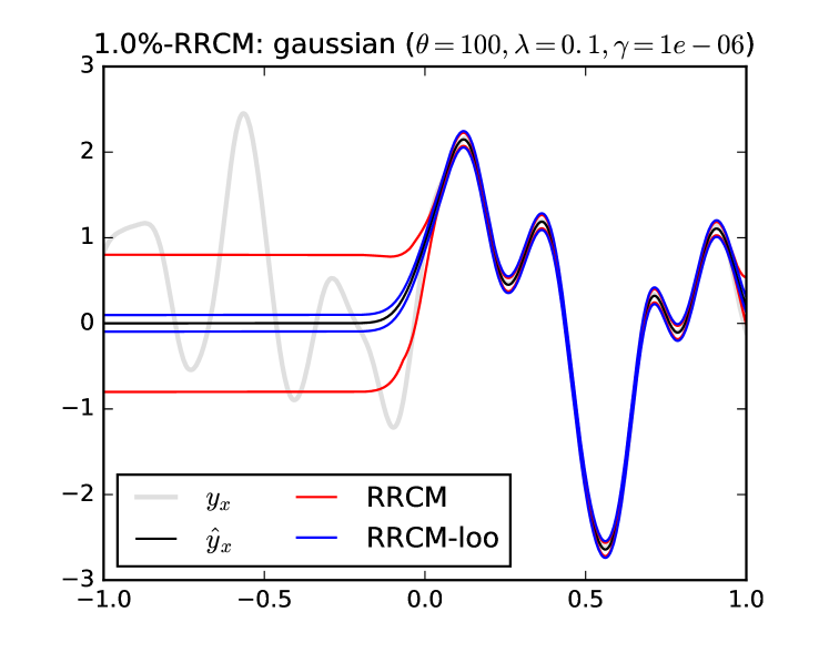
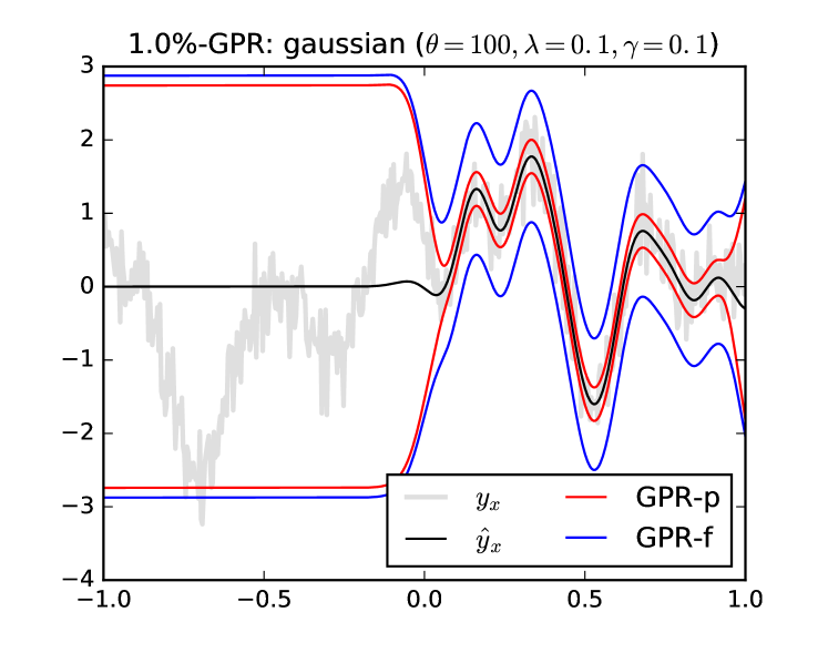
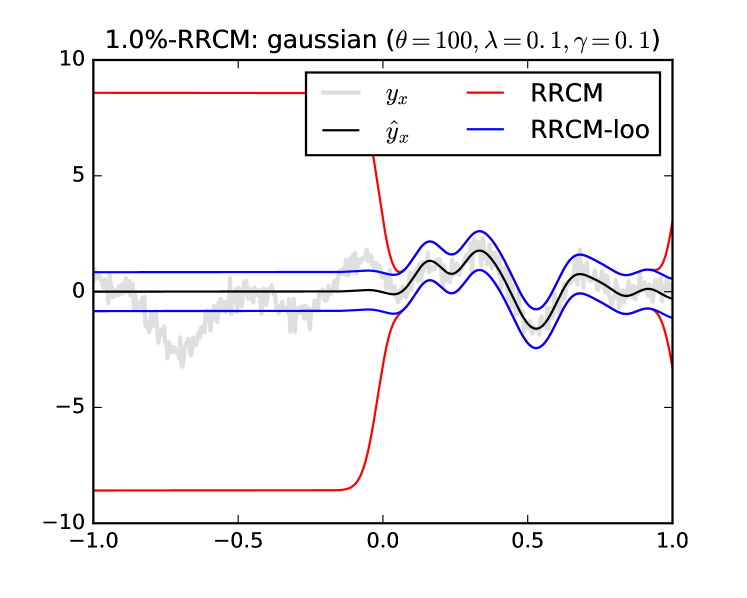
Figure 2: Limiting out-of-sample behaviour of GPR (left) and RRCM (right) confidence regions for a sample path of a Gaussian process with negligible (top, $\gamma=10^{-6}$) and high (bottom, $\gamma=10^{-1}$) noise-to-signal level.

Experimental results in the perfectly noiseless case show that both confidence regions are conservative (see fig. 3). In this picture we consider the ML estimate of $\theta$, but the results for other fixed choices are qualitatively similar. By construction, the procedure (eq. 6) adapts to the noise level in observations through the distribution of the non-conformity scores, rather than the regularization parameter $\lambda$, which makes Bayesian confidence intervals usually wider than conformal regions (fig. 3(b)). Nevertheless for higher $\lambda$ the coverage rate of conformal regions gets closer to the specified confidence level.

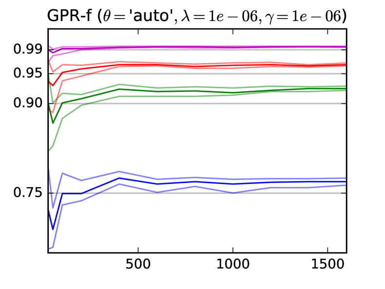
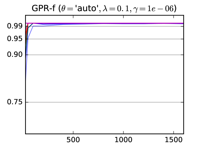
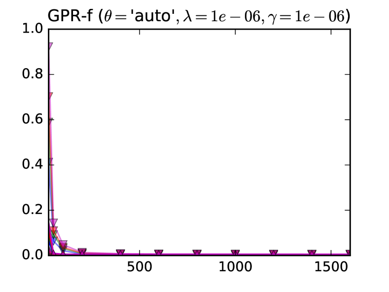
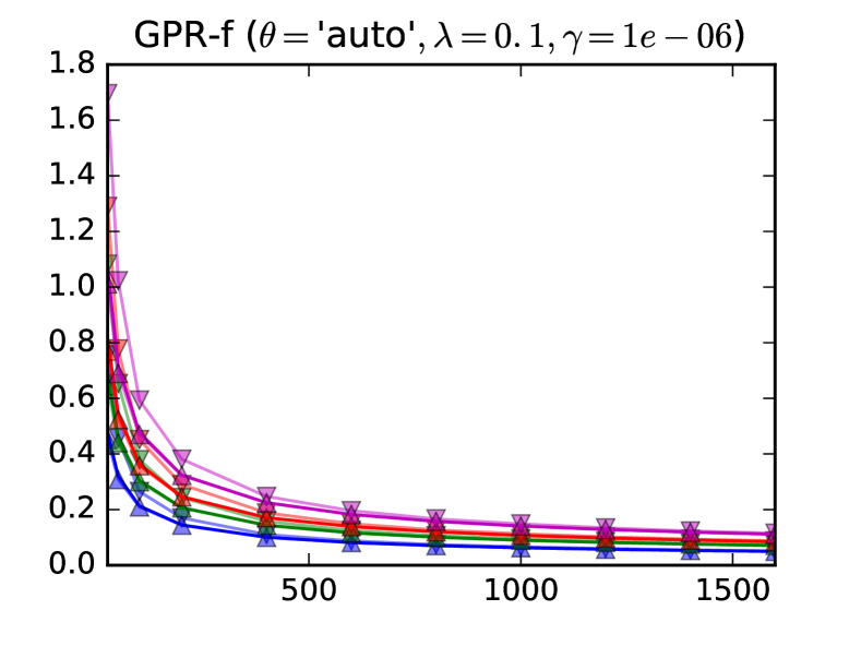
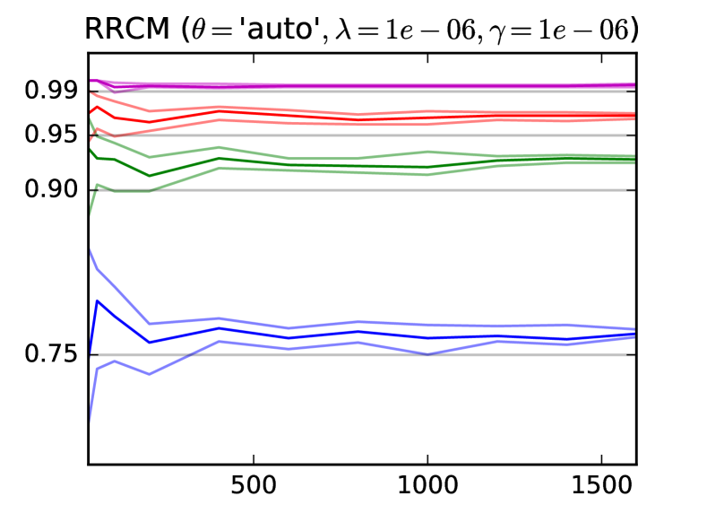
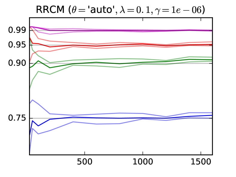
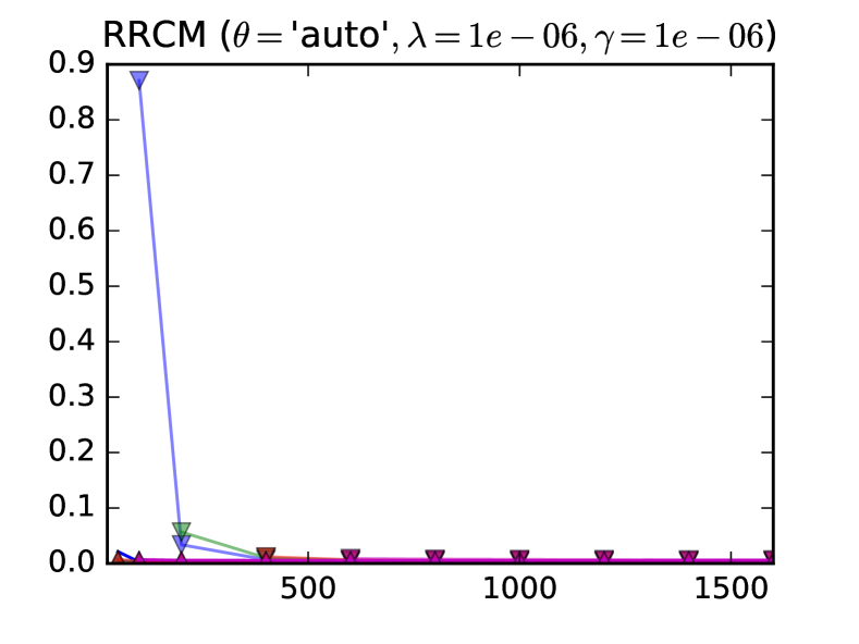
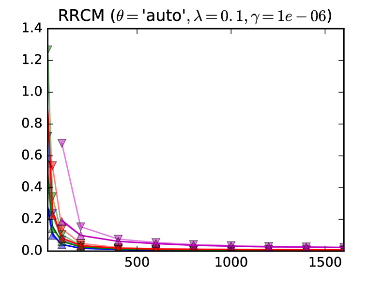
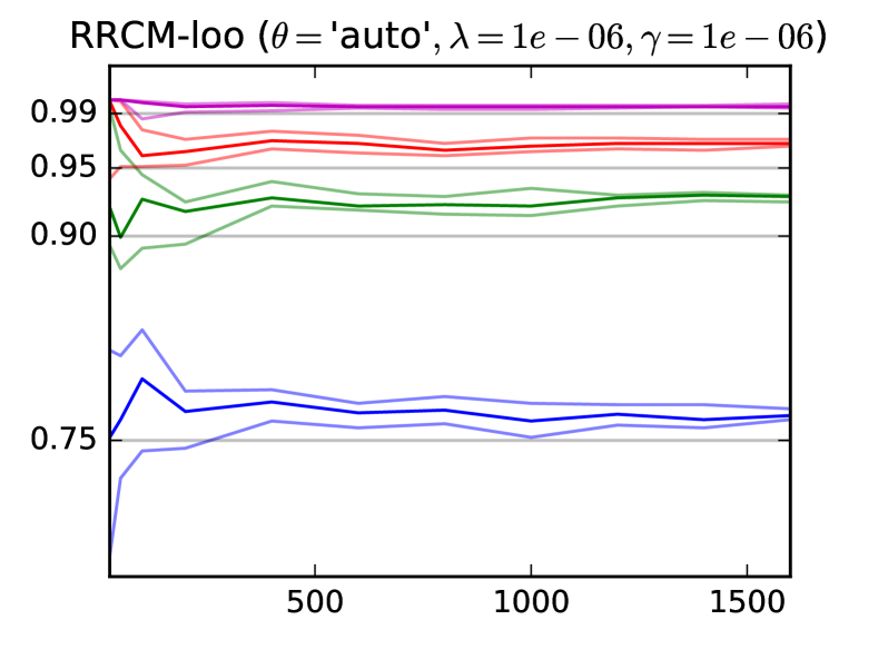
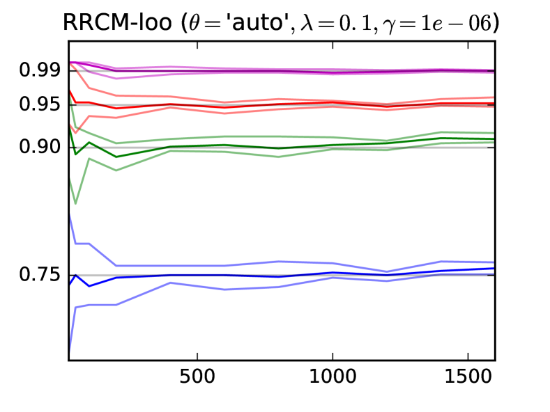
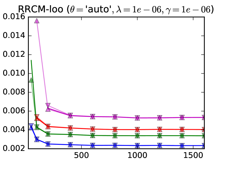
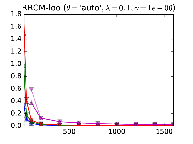
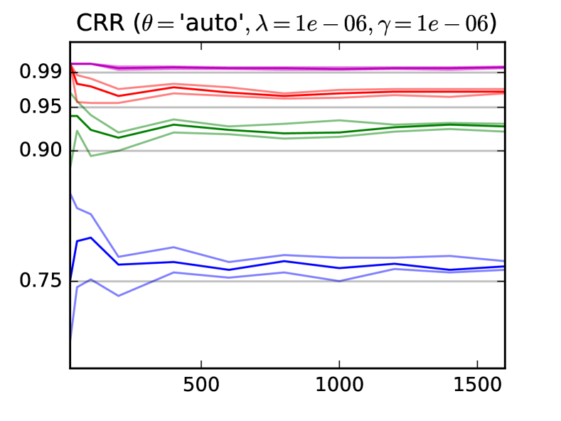
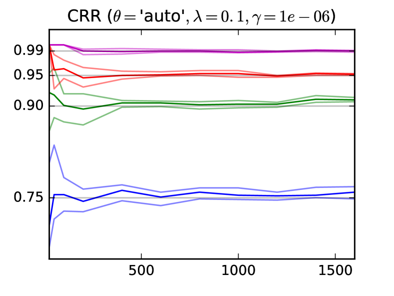
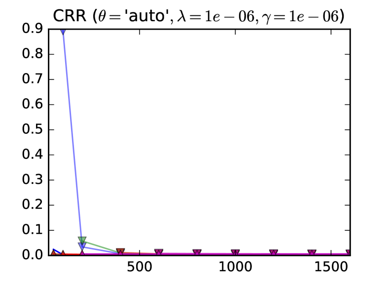
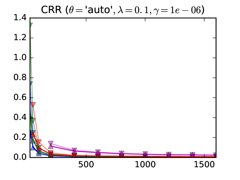
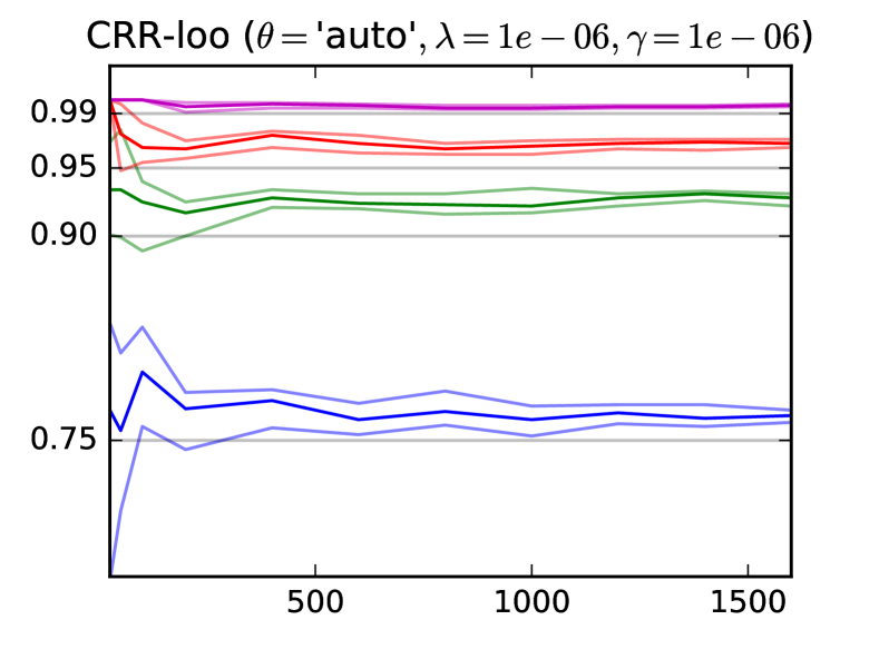
(a)

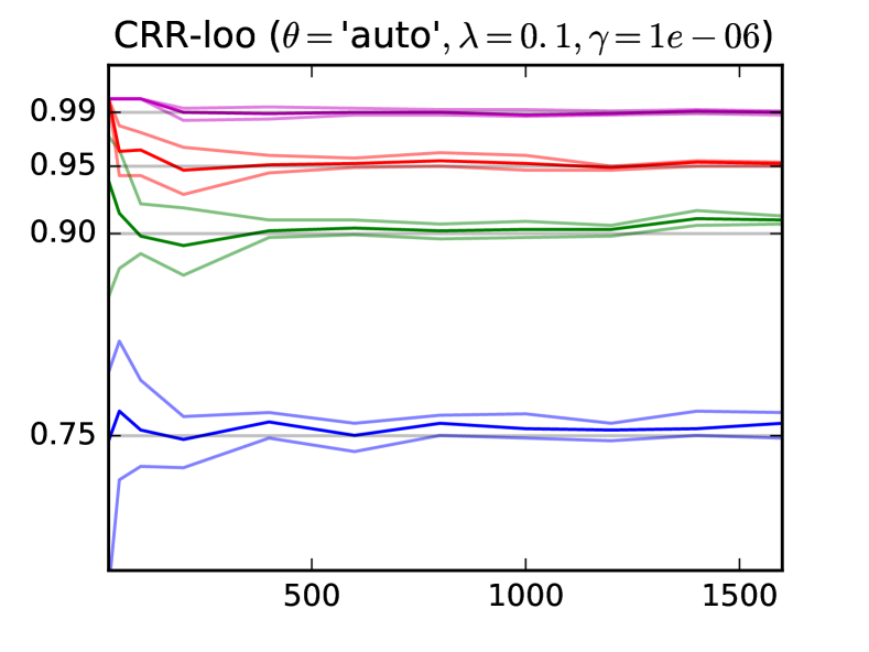
(b)

(c)

(d)

Figure 3: Coverage rate dynamics (3(a), 3(b)) and asymptotic width (3(c), 3(d)) of the confidence regions in the fully Gaussian low-noise case $\gamma=10^{-6}$ for $\theta=\hat{\theta}_{\text{ML}}$ and $\lambda=10^{-6}$ (3(a), 3(c)), and $\lambda=10^{-1}$ (3(b), 3(d)). Rows from top to bottom: ‘‘GPR-f’’, ‘‘RRCM’’, ‘‘RRCM-loo’’, ‘‘CRR’’, ‘‘CRR-loo’’. In columns 3(c) and 3(d) upward triangles indicate the $5\%$ sample quantile across the whole test sample, downward triangles indicate the maximal width, the median width is drawn with a slightly thicker line.

In the non-Gaussian noiseless experiments the coverage rate of conformal confidence intervals maintains approaches the specified confidence levels and all conformal procedures demonstrate very similar asymptotic validity. For the ‘‘Heaviside’’ step function typical confidence bands are shown in fig. 4, and the asymptotic coverage rate of various confidence bands are presented in fig. 5.

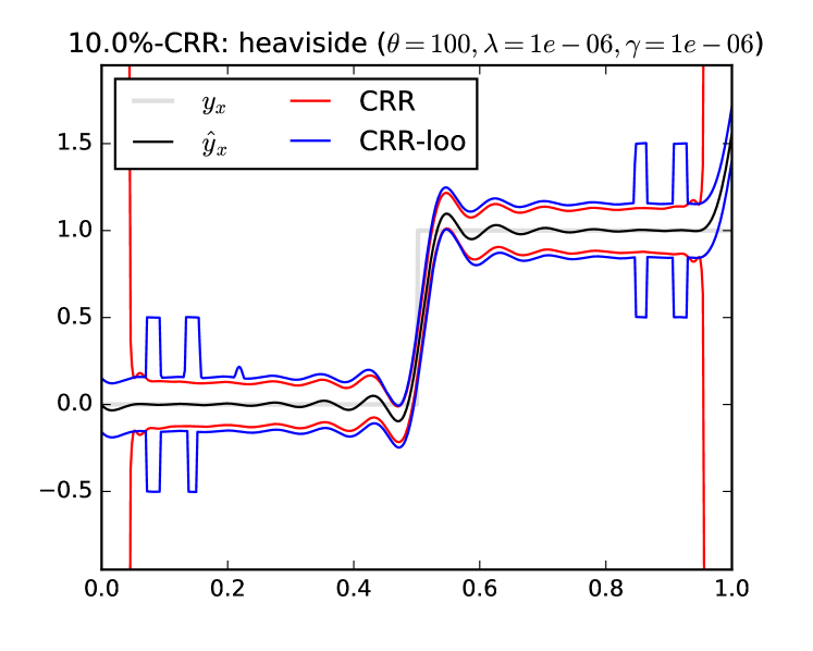
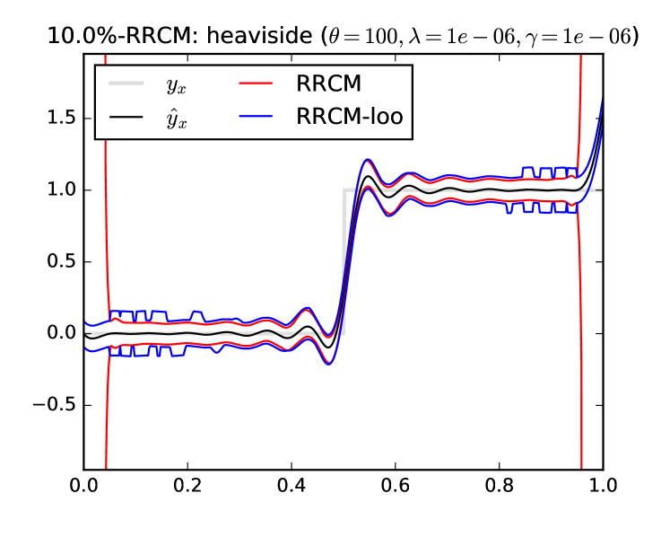
Figure 4: Typical conformal confidence bands for the ‘‘Heaviside’’ step function (train sample size $n=50$): left – CRR, and right – RRCM.

In the non-Gaussian setting the GPR confidence intervals are not consistently valid, as is evident from coverage rate dynamics for $\lambda=10^{-1}$. At the same time conformal procedures show no significant departures from claimed validity (results for other measures and residuals were qualitatively similar). The main conclusion is that in the negligible noise case the conformal confidence intervals for the KRR with the Gaussian kernel perform reasonably well both in terms of validity in a non-Gaussian setting and efficiency in fully Gaussian setting.

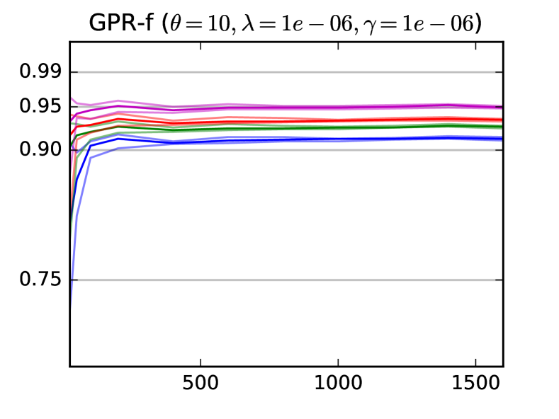
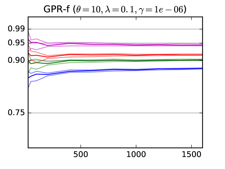
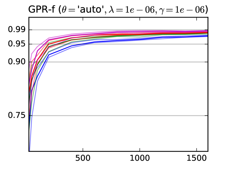
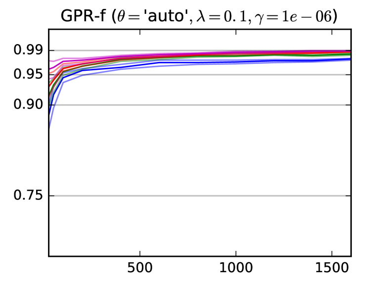
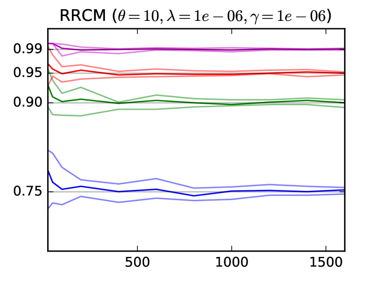
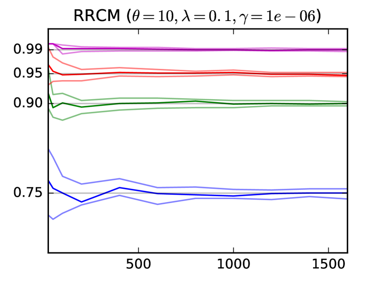
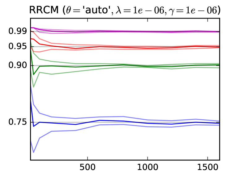
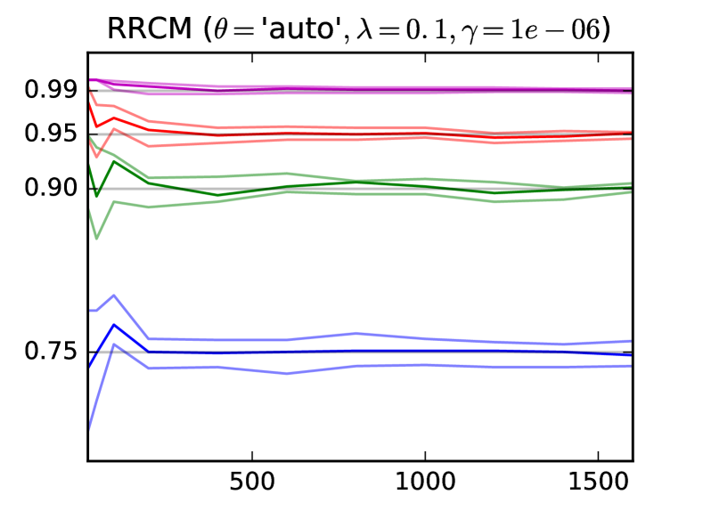
Figure 5: Coverage dynamics for the ‘‘Heaviside’’ ($\lambda=10^{-6}$).

The performance of conformal confidence regions in noisy setting ($\gamma=10^{-1}$) is qualitatively similar to the negligible nose case, except that the bands are wider due to higher observation noise. We report the findings for the MLE of $\theta$ only, but the results for conformal regions with fixed $\theta$ are qualitatively similar. In fig. 6 the conformal confidence regions provide the specified level of validity regardless of the parameter $\lambda$ of the non-conformity measure. As expected, the Bayesian confidence predictions uphold their theoretical guarantees.

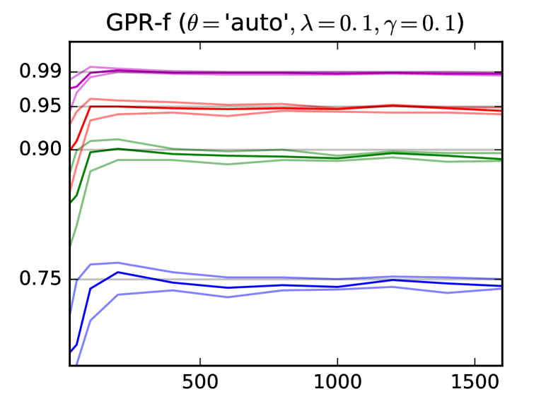
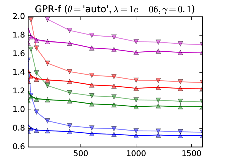
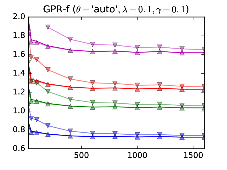
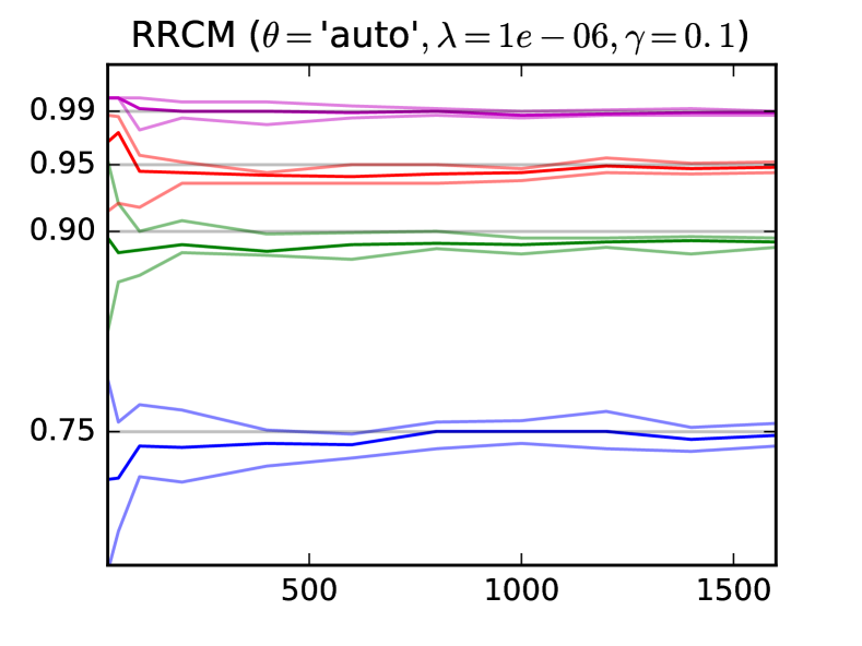
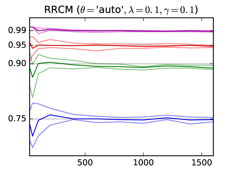
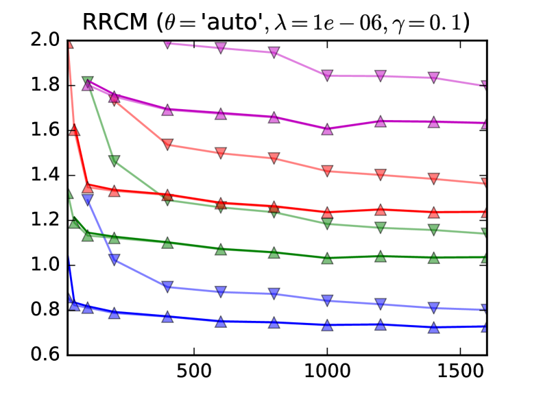
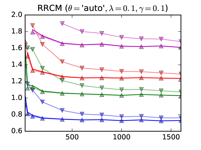
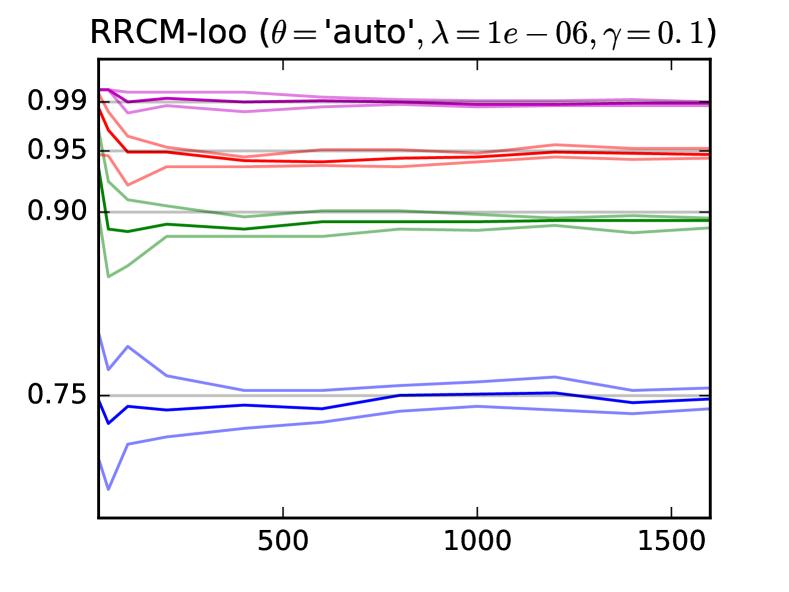
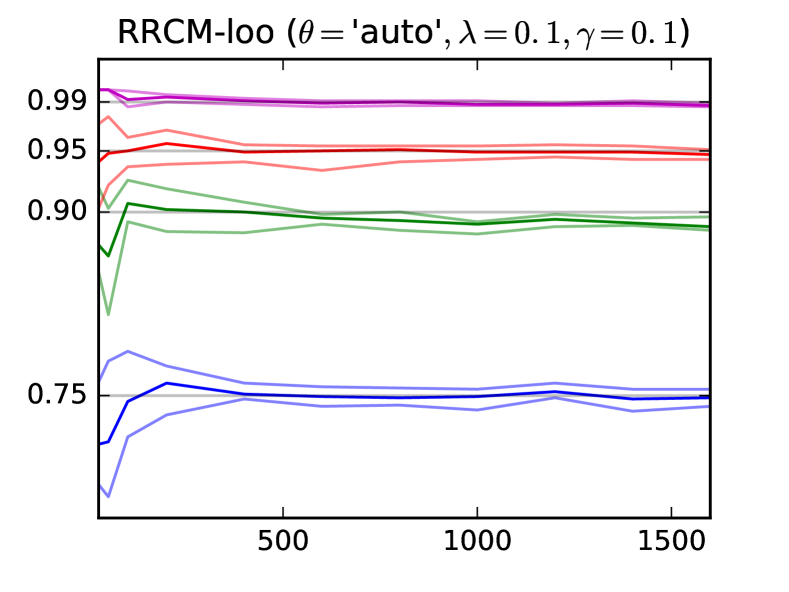
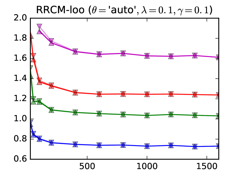
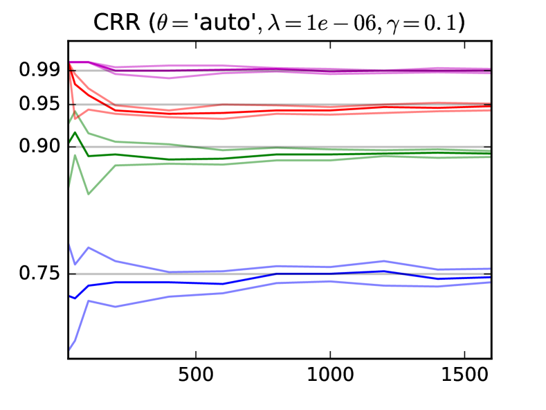
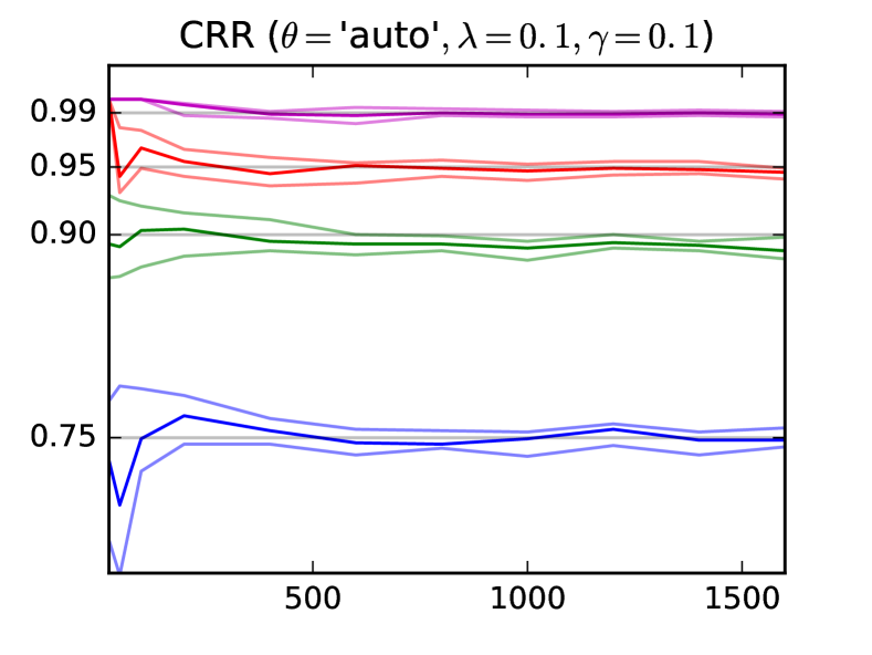
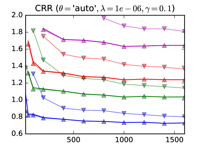
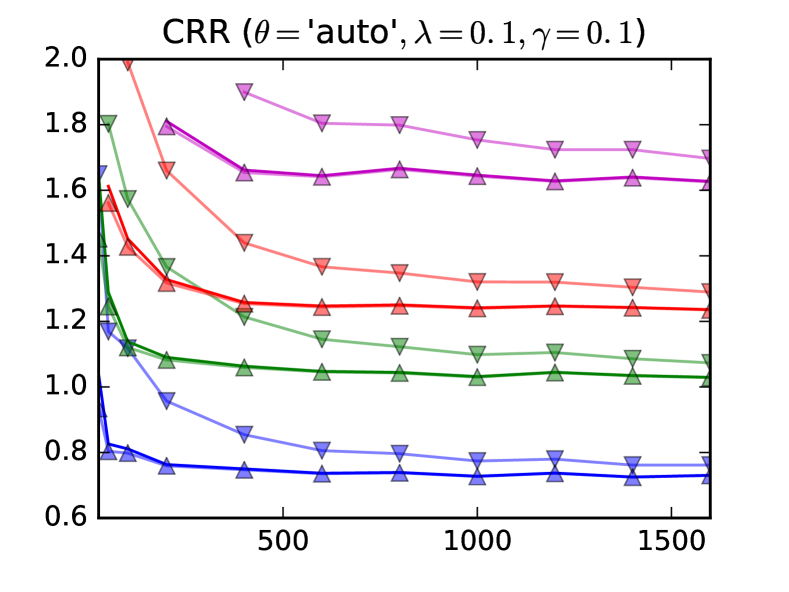
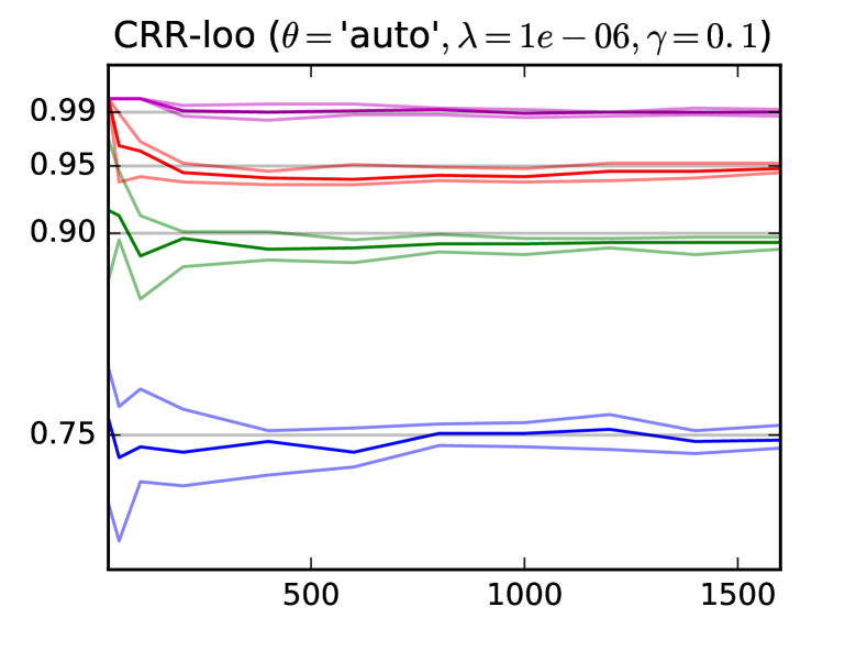
(a)

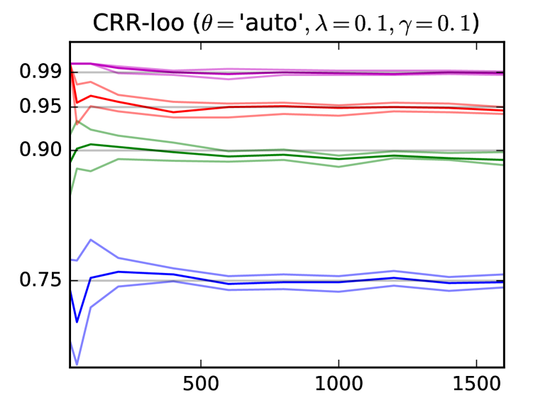
(b)

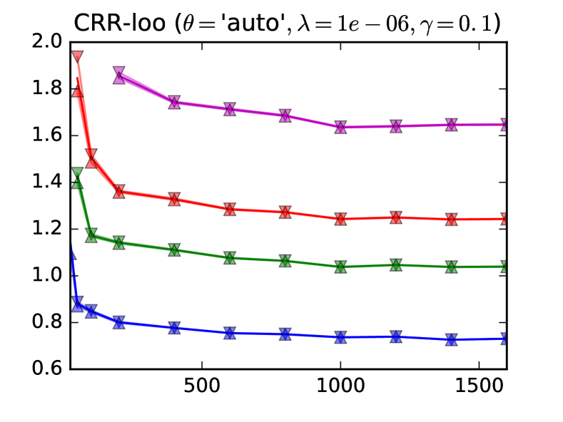
(c)

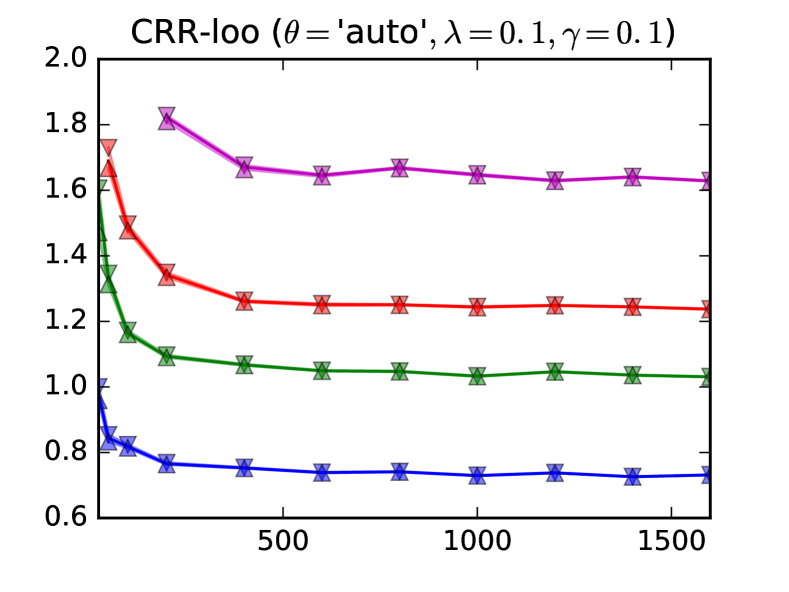
(d)

Figure 6: Coverage rate and region size dynamics in the noisy fully Gaussian case with $\gamma=10^{-1}$ for different $\theta=\hat{\theta}_{\text{ML}}$ and $\lambda=10^{-6}$ (6(a)), and $\lambda=10^{-1}$ (6(b)). Rows from top to bottom: ‘‘GPR-f’’, ‘‘RRCM’’, ‘‘RRCM-loo’’, ‘‘CRR’’, and ‘‘CRR-loo’’.

In the non-Gaussian setting with noise-to-signal ratio $\gamma=10^{-1}$, all experiments yielded results similar to the negligible noise case: the conformal confidence sets are asymptotically valid, whereas the Bayesian intervals are not, fig. 7.

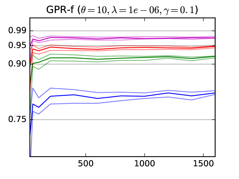
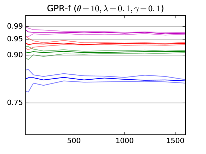
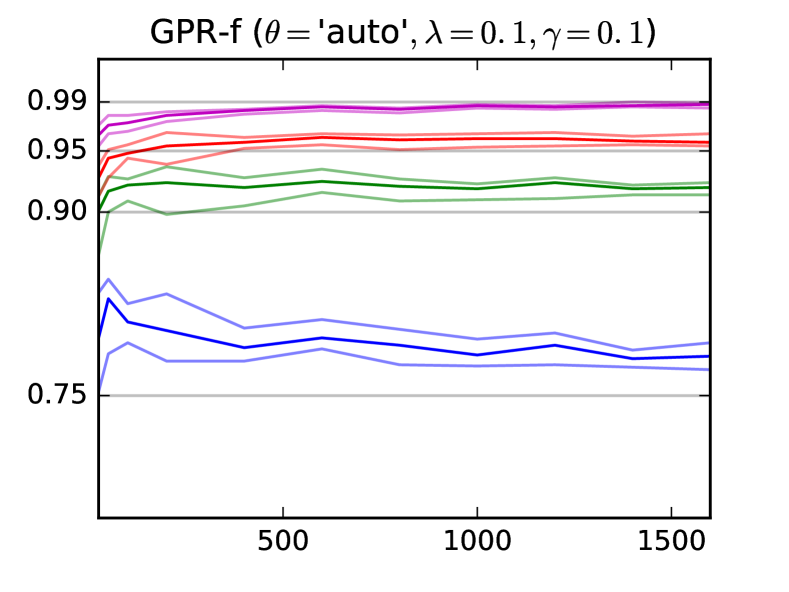
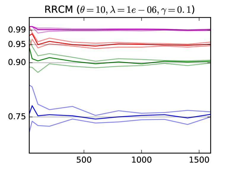
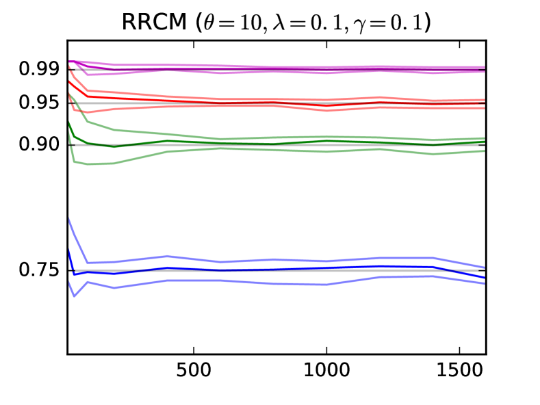
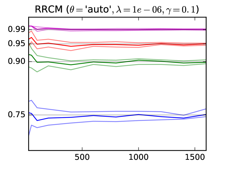
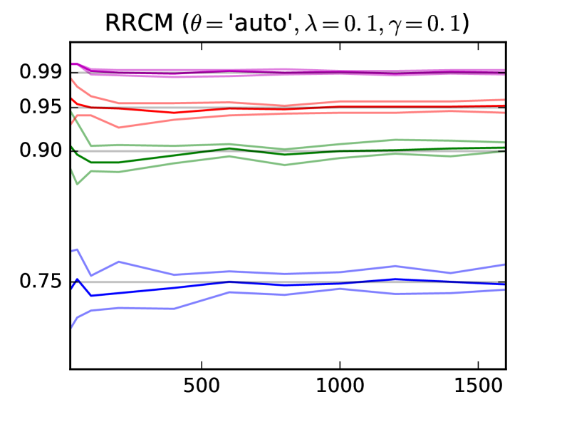
Figure 7: Coverage dynamics for the ‘‘Heaviside’’ ($\lambda=10^{-1}$).

IV-B Results: $2$-d

In this section we conduct experiments in the $2$-d setting $\mathcal{X}=[-1,1]^{2}$, and the experimental steps are similar to IV-A The typical sample realisations of the studied $2-d$ functions $f$ are depicted in fig. 8.

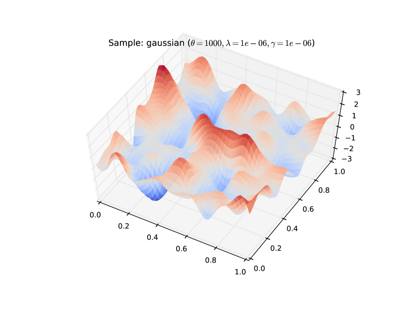
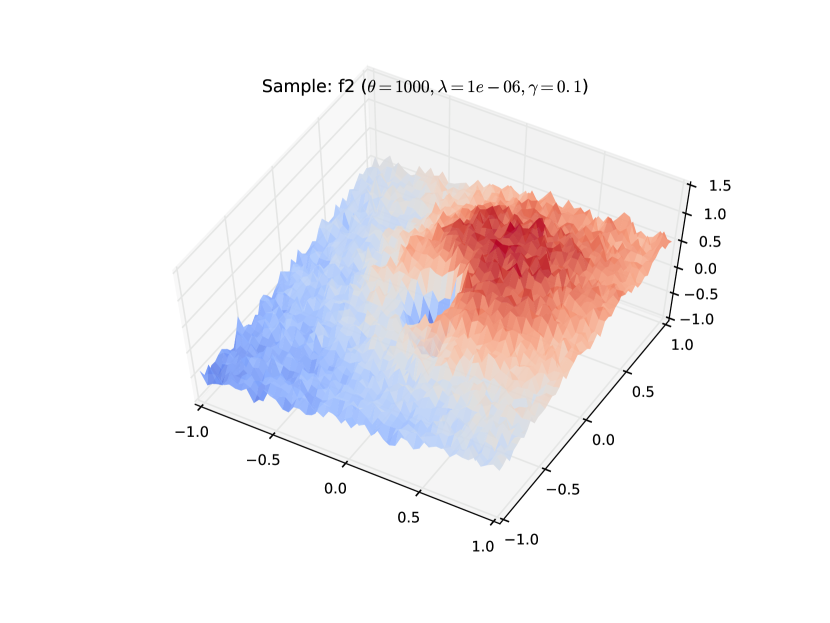
Figure 8: A sample path of a $2$-d Gaussian process(left $\gamma=10^{-6}$) and a non-Gaussian function ‘‘f2’’ (right $\gamma=10^{-1}$).

Table I shows the error rates ($y^{*}\notin\mathcal{B}(x^{*})$) of the Bayesian confidence intervals on the fixed test sample. Columns 1 and 4 show that the regions are approximately valid when the kernel and noise hyper-parameters are known. The Bayesian intervals are more conservative for the case of low noise ($\gamma=10^{-6}$) and high regularization $\lambda=10^{-1}$. However, the validity of the GPR confidence intervals is sensitive to misspecification of kernel precision $\theta$.

TABLE I: The empirical error rate ($\%$) of the GPR confidence interval for simulated $2$-d Gaussian process with train size $n=1500$.

	$\gamma$	$10^{-6}$		$10^{-1}$
	$\lambda$	$10^{-6}$	$10^{-1}$	$10^{-6}$	$10^{-1}$
$\theta$	$\alpha(\%)$
$10^{2}$	$1$	0.9	0.1	4.1	0.7
	$5$	4.5	0.5	12.0	4.4
	$10$	9.2	1.0	19.2	9.3
	$25$	23.8	3.3	36.1	24.5
$\hat{\theta}_{\text{ML}}$	$1$	0.8	0.1	2.3	0.8
	$5$	4.4	0.5	4.9	4.5
	$10$	9.0	0.9	8.0	9.4
	$25$	23.6	2.3	18.9	24.7
$10^{1}$	$1$	1.6	0.6	1.0	0.6
	$5$	5.3	4.2	5.2	3.7
	$10$	9.6	8.6	10.4	8.2
	$25$	22.5	23.4	26.3	22.6
$10^{3}$	$1$	0.4	0.4	9.1	1.1
	$5$	1.2	1.2	13.1	4.9
	$10$	2.0	2.0	16.1	9.6
	$25$	4.7	4.5	24.0	24.0

In contrast to the GPR confidence intervals, the conformal regions are insensitive to misspecification as demonstrated in table. II, where we show the maximal absolute deviation of the interval error rate from the specified rate $\alpha$ across all studied significance levels (eq. 21).

$$\mathtt{MAD}(\Gamma,A;\Theta)=\max_{\alpha\in A}\Bigl{\lvert}m^{-1}\#\{j\,:\,y^{*}_{j}\notin\Gamma^{\alpha}_{n}(X^{*}_{j};\Theta)\}-\alpha\Bigr{\rvert}\,,$$ (21)

where $\Theta$ is the vector of hyper-parameters of the experiment revealed to the conformal procedure, $A=\{1\%,5\%,10\%,25\%\}$, $(X^{*}_{j},y^{*}_{j})_{j=1}^{|X^{*}|}$ is the test sample.

TABLE II: The maximal absolute deviation $\mathtt{MAD}(\Gamma,A;\Theta)$ ($\%$) of the empirical error rate from the theoretical significance level of conformal confidence regions for simulated $2$-d Gaussian process for $n=1500$.

	$\gamma$	$10^{-6}$		$10^{-1}$
	$\lambda$	$10^{-6}$	$10^{-1}$	$10^{-6}$	$10^{-1}$
type	$\theta$
RRCM	$10^{1}$	0.3	0.2	0.8	0.4
	$10^{2}$	1.7	1.3	1.1	0.7
	$10^{3}$	1.1	2.6	1.2	0.5
	$\hat{\theta}_{\text{ML}}$	1.7	2.2	0.1	0.5
RRCM-loo	$10^{1}$	1.3	0.3	2.0	0.4
	$10^{2}$	2.4	1.7	2.0	0.4
	$10^{3}$	2.9	2.6	0.1	0.6
	$\hat{\theta}_{\text{ML}}$	2.6	2.6	0.8	0.6
CRR	$10^{1}$	0.3	0.1	0.8	0.3
	$10^{2}$	1.6	1.2	1.2	0.8
	$10^{3}$	0.8	2.2	1.3	0.5
	$\hat{\theta}_{\text{ML}}$	1.8	2.1	0.1	0.4
CRR-loo	$10^{1}$	1.2	0.3	2.0	0.2
	$10^{2}$	2.4	1.7	2.1	0.5
	$10^{3}$	2.6	2.4	0.3	0.5
	$\hat{\theta}_{\text{ML}}$	2.6	2.4	0.8	0.6

Typical profile of the test function used in non-Gaussian experiment is plotted in fig. 8 (p. 8). The performance of the conformal regions in the non-Gaussian experiments are summarized in tab. III. Overall, the error rates do not stray too far from the stated levels, and conformal regions are weakly sensitive to the KRR hyper-parameters. In contrast, tab. IV shows that the empirical error rate of Bayesian confidence intervals depends on the values of the precision parameter. The MLE $\theta$ produces conservatively valid confidence intervals, and for $\gamma=10^{-1}$ the error rate becomes closer to the specified significance level.

TABLE III: The maximal absolute deviation $\mathtt{MAD}(\Gamma,A;\Theta)$ ($\%$) of the empirical error rate from the theoretical significance level of conformal confidence regions for the ‘‘f2’’ test function ($n=1500$).

	$\gamma$	$10^{-6}$		$10^{-1}$
	$\lambda$	$10^{-6}$	$10^{-1}$	$10^{-6}$	$10^{-1}$
type	$\theta$
CRR	$10^{1}$	1.0	1.3	1.2	0.2
	$10^{2}$	0.7	2.7	1.4	0.6
	$10^{3}$	0.3	1.1	1.0	0.1
	$\hat{\theta}_{\text{ML}}$	1.4	2.2	0.6	0.5
CRR-loo	$10^{1}$	0.8	1.4	1.3	0.2
	$10^{2}$	3.0	3.2	1.9	0.5
	$10^{3}$	1.0	1.0	0.2	0.2
	$\hat{\theta}_{\text{ML}}$	2.6	2.6	0.5	0.2
RRCM	$10^{1}$	0.9	1.4	1.2	0.2
	$10^{2}$	0.7	2.6	1.3	0.6
	$10^{3}$	0.4	0.5	0.9	0.3
	$\hat{\theta}_{\text{ML}}$	1.3	2.3	0.8	0.4
RRCM-loo	$10^{1}$	0.8	1.6	1.2	0.3
	$10^{2}$	3.0	3.2	2.0	0.6
	$10^{3}$	0.9	0.6	0.2	0.2
	$\hat{\theta}_{\text{ML}}$	2.6	2.6	0.7	0.1

TABLE IV: The empirical error rate ($\%$) of the GPR confidence interval for the ‘‘f2’’ test function ($n=1500$).

	$\gamma$	$10^{-6}$		$10^{-1}$
	$\lambda$	$10^{-6}$	$10^{-1}$	$10^{-6}$	$10^{-1}$
$\theta$	$\alpha(\%)$
$10^{1}$	$1\%$	2.3	1.9	2.2	1.1
	$5\%$	3.2	3.0	7.9	4.9
	$10\%$	4.0	3.7	13.8	9.7
	$25\%$	5.8	5.6	29.9	24.3
$10^{2}$	$1\%$	0.3	0.0	19.1	1.3
	$5\%$	0.6	0.1	28.6	5.9
	$10\%$	0.9	0.2	35.0	11.1
	$25\%$	2.6	1.2	48.3	26.5
$10^{3}$	$1\%$	0.1	0.1	2.4	0.1
	$5\%$	1.9	2.1	4.0	1.9
	$10\%$	4.1	4.5	6.0	5.0
	$25\%$	12.9	13.4	13.9	16.4
$\hat{\theta}_{\text{ML}}$	$1\%$	3.4	0.6	2.0	1.1
	$5\%$	4.4	1.1	3.9	5.1
	$10\%$	5.2	1.4	6.9	10.0
	$25\%$	7.1	2.4	18.1	24.9

V Conclusion

Experiments in sec. IV provide evidence suggesting that conformal procedures are insensitive to the choice of the core NCM and are asymptotically equivalent in terms of coverage and efficiency, despite being applied in the off-line batch learning setting. Furthermore, the results indicate that both Bayesian and conformal confidence intervals possess the asymptotic validity guarantees, when the Gaussian assumptions hold, and the conformal procedure yields asymptotically efficient regions.

Further research shall focus on establishing theoretical foundations for the obtained experimental results for the KRR with Gaussian kernel, or isolating special cases when it holds, and studying the cases when it fails, and generalizing the efficiency result in [23].

References

- [1] S. Alestra, E. Burnaev, C. Bordry, C. Brand, P. Erofeev, A. Papanov, and C. Silveira-Freixo, ‘‘Application of rare event anticipation techniques to aircraft health management,’’ in Mechanical and Aerospace Engineering V, ser. Advanced Materials Research, vol. 1016. Trans Tech Publications, 11 2014, pp. 413–417.
- [2] E. Burnaev, P. Erofeev, and D. Smolyakov, ‘‘Model selection for anomaly detection,’’ pp. 987 525–987 525–6, 2015. [Online]. Available: http://dx.doi.org/10.1117/12.2228794
- [3] A. Artemov, E. Burnaev, and A. Lokot, ‘‘Nonparametric decomposition of quasi-periodic time series for change-point detection,’’ pp. 987 520–987 520–5, 2015. [Online]. Available: http://dx.doi.org/10.1117/12.2228370
- [4] C. C. Aggarwal and S. Y. Philip, ‘‘Outlier detection with uncertain data.’’ in Proceedings of the SIAM International Conference on Data Mining. SIAM, 2008, pp. 483–493.
- [5] D. W. Scott, ‘‘Kernel density estimators,’’ Multivariate Density Estimation: Theory, Practice, and Visualization, pp. 125–193, 2008.
- [6] V. Hautamaki, I. Karkkainen, and P. Franti, ‘‘Outlier detection using k-nearest neighbour graph,’’ in Proceedings of the Pattern Recognition, 17th International Conference on (ICPR’04) Volume 3 - Volume 03, ser. ICPR ’04. Washington, DC, USA: IEEE Computer Society, 2004, pp. 430–433. [Online]. Available: http://dx.doi.org/10.1109/ICPR.2004.671
- [7] M. M. Breunig, H.-P. Kriegel, R. T. Ng, and J. Sander, ‘‘Lof: Identifying density-based local outliers,’’ SIGMOD Rec., vol. 29, no. 2, pp. 93–104, May 2000. [Online]. Available: http://doi.acm.org/10.1145/335191.335388
- [8] H.-P. Kriegel, P. Kröger, E. Schubert, and A. Zimek, ‘‘Loop: Local outlier probabilities,’’ in Proceedings of the 18th ACM Conference on Information and Knowledge Management, ser. CIKM ’09. New York, NY, USA: ACM, 2009, pp. 1649–1652. [Online]. Available: http://doi.acm.org/10.1145/1645953.1646195
- [9] M. F. Augusteijn and B. A. Folkert, ‘‘Neural network classification and novelty detection,’’ International Journal of Remote Sensing, vol. 23, no. 14, pp. 2891–2902, 2002. [Online]. Available: http://www.tandfonline.com/doi/abs/10.1080/01431160110055804
- [10] S. Hawkins, H. He, G. J. Williams, and R. A. Baxter, ‘‘Outlier detection using replicator neural networks,’’ in Data Warehousing and Knowledge Discovery: 4th International Conference, DaWaK 2002 Aix-en-Provence, France, September 4–6, 2002 Proceedings, ser. DaWaK 2000, Y. Kambayashi, W. Winiwarter, and M. Arikawa, Eds. Berlin, Heidelberg: Springer Berlin Heidelberg, 2002, pp. 170–180. [Online]. Available: http://dx.doi.org/10.1007/3-540-46145-0_17
- [11] H. Hoffmann, ‘‘Kernel pca for novelty detection,’’ Pattern Recogn., vol. 40, no. 3, pp. 863–874, Mar. 2007. [Online]. Available: http://dx.doi.org/10.1016/j.patcog.2006.07.009
- [12] B. Schölkopf, A. Smola, and K.-R. Müller, ‘‘Nonlinear component analysis as a kernel eigenvalue problem,’’ Neural Comput., vol. 10, no. 5, pp. 1299–1319, Jul. 1998. [Online]. Available: http://dx.doi.org/10.1162/089976698300017467
- [13] A. Bernstein, A. Kuleshov, and Y. Yanovich, Manifold Learning in Regression Tasks. Cham: Springer International Publishing, 2015, pp. 414–423. [Online]. Available: http://dx.doi.org/10.1007/978-3-319-17091-6_36
- [14] A. Kuleshov and A. Bernstein, Extended Regression on Manifolds Estimation. Cham: Springer International Publishing, 2016, pp. 208–228. [Online]. Available: http://dx.doi.org/10.1007/978-3-319-33395-3_15
- [15] B. Schölkopf and A. Smola, Learning with Kernels: Support Vector Machines, Regularization, Optimization, and Beyond, ser. Adaptive computation and machine learning. MIT Press, 2002.
- [16] C. Rasmussen and C. Williams, Gaussian Processes for Machine Learning, ser. Adaptative computation and machine learning series. University Press Group Limited, 2006.
- [17] E. V. Burnaev, A. A. Zaytsev, and V. G. Spokoiny, ‘‘The bernstein-von mises theorem for regression based on gaussian processes,’’ Russian Mathematical Surveys, vol. 68, no. 5, p. 954, 2013. [Online]. Available: http://dx.doi.org/10.1070/RM2013v068n05ABEH004863
- [18] A. A. Zaitsev, E. V. Burnaev, and V. G. Spokoiny, ‘‘Properties of the posterior distribution of a regression model based on gaussian random fields,’’ Automation and Remote Control, vol. 74, no. 10, pp. 1645–1655, 2013. [Online]. Available: http://dx.doi.org/10.1134/S0005117913100056
- [19] M. Belyaev, E. Burnaev, and Y. Kapushev, Gaussian Process Regression for Structured Data Sets. Cham: Springer International Publishing, 2015, pp. 106–115. [Online]. Available: http://dx.doi.org/10.1007/978-3-319-17091-6_6
- [20] ——, ‘‘Computationally efficient algorithm for gaussian process regression in case of structured samples,’’ Computational Mathematics and Mathematical Physics, vol. 56, no. 4, pp. 499–513, 2016. [Online]. Available: http://dx.doi.org/10.1134/S0965542516040163
- [21] E. V. Burnaev, M. E. Panov, and A. A. Zaytsev, ‘‘Regression on the basis of nonstationary gaussian processes with bayesian regularization,’’ Journal of Communications Technology and Electronics, vol. 61, no. 6, pp. 661–671, 2016. [Online]. Available: http://dx.doi.org/10.1134/S1064226916060061
- [22] V. Vovk, A. Gammerman, and G. Shafer, Algorithmic Learning in a Random World. Springer, 2005.
- [23] E. Burnaev and V. Vovk, ‘‘Efficiency of conformalized ridge regression,’’ in Proceedings of The 27th Conference on Learning Theory, COLT 2014, Barcelona, Spain, June 13-15, 2014, 2014, pp. 605–622. [Online]. Available: http://jmlr.org/proceedings/papers/v35/burnaev14.html