Weak solution of a continuum model for vicinal surface in the attachment-detachment-limited regime

Abstract.

We study in this work a continuum model derived from 1D attachment-detachment-limited (ADL) type step flow on vicinal surface,

$$u_{t}=-u^{2}(u^{3})_{hhhh},$$

where $u$, considered as a function of step height $h$, is the step slope of the surface. We formulate a notion of weak solution to this continuum model and prove the existence of a global weak solution, which is positive almost everywhere. We also study the long time behavior of weak solution and prove it converges to a constant solution as time goes to infinity. The space-time Hölder continuity of the weak solution is also discussed as a byproduct.

1. Introduction

During the heteroepitaxial growth of thin films, the evolution of the crystal surfaces involves various structures. Below the roughening transition temperature, the crystal surface can be well characterized as steps and terraces, together with adatoms on the terraces. Adatoms detach from steps, diffuse on the terraces until they meet one of the steps and reattach again, which lead to a step flow on the crystal surface. The evolution of individual steps is described mathematically by the Burton-Cabrera-Frank (BCF) type models [3]; see [5, 6] for extensions to include elastic effects. Denote the step locations at time $t$ by $x_{i}(t),i\in\mathbb{Z}$, where $i$ is the index of the steps. Denote the height of each step as $a$. For one dimensional vicinal surface (i.e., monotone surface), if we do not consider the deposition flux, the original BCF type model, after non-dimensionalization, can be written as (we set some physical constants to be $1$ for simplicity):

(1.1) $$\dot{x}_{i}=\frac{D}{ka^{2}}\bigg{(}\frac{\mu_{i+1}-\mu_{i}}{x_{i+1}-x_{i}+\frac{D}{k}}-\frac{\mu_{i}-\mu_{i-1}}{x_{i}-x_{i-1}+\frac{D}{k}}\bigg{)},\text{ for }1\leq i\leq N.$$

where $D$ is the terrace diffusion constant, $k$ is the hopping rate of an adatom to the upward or downward step, and $\mu$ is the chemical potential whose expression ranges under different assumption. Often two limiting cases of the classical BCF type model (1.1) were considered. See [26, 16] for diffusion-limited (DL) case and see [13, 1] for attachment-detachment-limited (ADL) case.

In DL regime, the dominated dynamics is diffusion across the terraces, i.e. $\frac{D}{k}<<x_{i+1}-x_{i}$, so the step-flow ODE becomes

(1.2) $$\dot{x}_{i}=\frac{D}{ka^{2}}\bigg{(}\frac{\mu_{i+1}-\mu_{i}}{x_{i+1}-x_{i}}-\frac{\mu_{i}-\mu_{i-1}}{x_{i}-x_{i-1}}\bigg{)},\text{ for }1\leq i\leq N.$$

In ADL regime, the diffusion across the terraces is fast, i.e. $\frac{D}{k}>>x_{i+1}-x_{i}$, so the dominated processes are the exchange of atoms at steps edges, i.e., attachment and detachment. The step-flow ODE in ADL regime becomes

(1.3) $$\dot{x_{i}}=\frac{1}{a^{2}}\big{(}\mu_{i+1}-2\mu_{i}+\mu_{i-1}\big{)},\text{ for }1\leq i\leq N.$$

Those models are widely used for crystal growth of thin films on substrates; see many scientific and engineering applications in the books [23, 28, 32]. As many of the film’s properties and performances originate in their growth processes, understanding and mastering thin film growth is one of the major challenges of materials science.

Although these mesoscopic models provide details of discrete nature, continuum approximation for the discrete models is also used to analyze the step motion. They involve fewer variables than discrete models so they can reveal the leading physics structure and are easier for numerical simulation. Many interesting continuum models can be found in the literature on surface morphological evolution; see [22, 25, 7, 29, 30, 24, 20, 4, 10] for one dimensional models and [19, 31] for two dimensional models. The study of relation between the discrete ODE models and the corresponding continuum PDE has raised lots of interest. Driven by this goal, it is important to understand the well-posedness and properties of the solutions to those continuum models.

For a general surface with peaks and valleys, the analysis of step motion on the level of continuous PDE is complicated so we focus on a simpler situation in this work: a monotone one-dimensional step train, known as the vicial surface in physics literature. In this case, Ozdemir, Zangwill [22] and Al Hajj Shehadeh, Kohn and Weare [1] realized using the step slope as a new variable is a convenient way to derive the continuum PDE model

(1.4) $$u_{t}=-u^{2}(u^{3})_{hhhh},$$

where $u$, considered as a function of step height $h$, is the step slope of the surface. We validate this continuum model by formulating a notion of weak solution. Then we prove the existence of such a weak solution. The weak solution is also persistent, i.e., it is positive (or negative) almost everywhere if non-negative (or non-positive) initial data are assumed.

The starting point of this PDE is the 1D attachment-detachment-limited (ADL) type models (1.3). To simplify the analysis, we will consider a periodic train of steps in this work, i.e., we assume that

(1.5) $$x_{i+N}(t)-x_{i}(t)=L,\qquad\forall\,i\in\mathbb{Z},\,\forall\,t\geq 0,$$

where $L$ is a fixed length of the period. Thus, only the step locations in one period $\{x_{i}(t),\,i=1,\ldots,N\}$ are considered as degrees of freedom. Since the vicinal surface is very large in practice from the microscopic point of view, this is a good approximation. We set the height of each step as $a=\frac{1}{N}$, and thus the total height changes across the $N$ steps in one period is given by $1$. This choice is suitable for the continuum limit $N\rightarrow\infty$. See Figure 1 for an example of step train in one period.

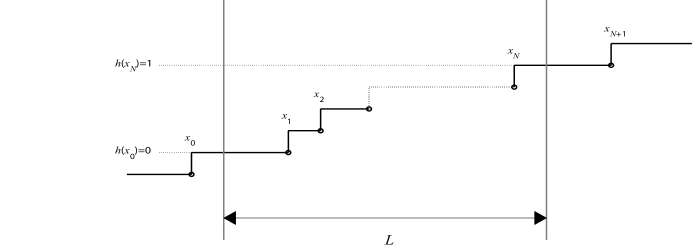
Figure 1. An example of step configurations with periodic boundary condition.

The general form of the (free) energy functional due to step interaction is

(1.6) $$F_{N}=a\sum_{i=0}^{N-1}f\big{(}\frac{x_{i+1}-x_{i}}{a}\big{)},$$

where $f$ reflects the physics of step interaction. Following the convention in focusing on entropic and elastic-dipoles interaction [21, 14], we choose $f(r)=\frac{1}{2r^{2}}$. Hence each step evolves by (1.3) with chemical potential $\mu_{i}$ defined as the first variation of the step interaction energy

(1.7) $$F_{N}=\frac{1}{2}\sum_{i=0}^{N-1}\frac{a^{3}}{(x_{i+1}-x_{i})^{2}},$$

with respect to $x_{i}.$ That is

(1.8) $$\mu_{i}=\frac{1}{a}\frac{\partial F_{N}}{\partial x_{i}}=\frac{a^{2}}{(x_{i+1}-x_{i})^{3}}-\frac{a^{2}}{(x_{i}-x_{i-1})^{3}},\text{ for }1\leq i\leq N.$$

From the periodicity of $x_{i}$ in (1.5), it is easy to see the periodicity of $\mu$ such that $\mu_{i}=\mu_{i+N}.$

When the step height $a\to 0$ or equivalently, the number of steps in one period $N\to\infty$, from the viewpoint of surface slope, Al Hajj Shehadeh, Kohn and Weare [1] and Margetis, Nakamura [20] studied the continuum model (1.4); see also [22] for physical derivation in general case. We recall their ideas in our periodic setup. Denote the step slopes as

$$u_{i}(t)=\frac{a}{x_{i+1}(t)-x_{i}(t)},\text{ for }1\leq i\leq N.$$

The periodicity of $x_{i}$ in (1.5) directly implies the periodicity of $u_{i}$, i.e. $u_{i}=u_{i+N}.$ Then by straight-forward calculation, we have the ODE for slopes

(1.9) $$\dot{u}_{i}=-\frac{1}{a^{4}}u_{i}^{2}\Big{[}(u_{i+2}^{3}-2u_{i+1}^{3}+u_{i}^{3})-2(u_{i+1}^{3}-2u_{i}^{3}+u_{i-1}^{3})+(u_{i}^{3}-2u_{i-1}^{3}+u_{i-2}^{3})\Big{]}.$$

Under the periodic setup, when considering step slope $u$ as a function of $h$ in continuum model, $u$ has period $1$. Keep in mind the height of each step $x_{i}$ is $h_{i}=ia.$ It is natural to anticipate that as $N\rightarrow\infty,$ the solution of the slope ODE (1.9) should converge to the solution $u(h,t)$ of continuum model (1.4), which is 1-periodic with respect to step height $h$.

By different methods, [1] and [20] separately studied the self-similar solution of ODE (1.9) and PDE (1.4). For monotone initial data, i.e. $x_{1}(0)<x_{2}(0)<\cdots<x_{N}(0)$, [1] proved the steps do not collide and the global-in-time solution to ODE (1.9) (as well as ODE (1.3)) was obtained in their paper. By introducing a similarity variable, [1] first discovered that the self-similar solution is a critical point of a “similarity energy”, for both discrete and continuum systems. Then they rigorously prove the continuum limit of self-similar solution and obtained the convergence rate for self-similar solution.

However, as far as we know, the global-in-time validation of the time-dependent continuum limit model (1.4) is still an open question as stated in [15]. In fact, it is not even known whether (1.4) has a well-defined, unique solution. Although the positivity of solution to continuum model (1.4) corresponds to the non-collision of steps in discrete model, which was proved in [1]; even a “formal proof” of positive global weak solution in the time-dependent continuous setting has not been established.

Our goal is to formulate a notion of weak solution and prove the existence of global weak solution. We also prove the almost everywhere positivity of the solution, which might help the study of global convergence of discrete model (1.3) to its continuum limit (1.4) in the future. Moreover, we study the long time behavior of weak solutions and prove that all weak solutions converge to a constant as time goes to infinity. The space-time Hölder continuity of the solution is also obtained.

One of the key structures of the model is that it possesses the following two Lyapunov functions,

(1.10) $$F{(u)}:=\frac{1}{2}\int_{0}^{1}u^{2}\,\mathrm{d}h,$$

and

(1.11) $$E{(u)}:=\int_{0}^{1}\frac{1}{6}[(u^{3})_{hh}]^{2}\,\mathrm{d}h.$$

Then we have

$$\frac{\delta F{(u)}}{\delta u}=u,\quad\frac{\delta E{(u)}}{\delta u}=u^{2}(u^{3})_{hhhh},$$

and (1.4) can be recast as

(1.12) $$u_{t}=-\frac{\delta E{(u)}}{\delta u}=-u^{2}\partial_{hhhh}\Big{(}u^{2}\frac{\delta F{(u)}}{\delta u}\Big{)}.$$

Since the homogeneous degree of $E(u)$ is $6$, one has

$$6E(u)=\int_{0}^{1}u\frac{\delta E(u)}{\delta u}\,\mathrm{d}h.$$

Then by (1.12),we obtain

(1.13) $$\frac{\,\mathrm{d}F(u)}{\,\mathrm{d}t}+6E(u)=\int_{0}^{1}u\big{(}u_{t}+\frac{\delta E(u)}{\delta u}\big{)}\,\mathrm{d}h=0.$$

Notice that

(1.14) $$\frac{\,\mathrm{d}E{(u)}}{\,\mathrm{d}t}=\int_{0}^{1}\frac{\delta E{(u)}}{\delta u}u_{t}\,\mathrm{d}h=-\int_{0}^{1}u_{t}^{2}\,\mathrm{d}h\leq 0.$$

Therefore, we also have the following dissipation structures:

(1.15) $$\frac{\,\mathrm{d}E(u)}{\,\mathrm{d}t}+D(u)=0,$$

where $D:=\int_{0}^{1}[u^{2}(u^{3})_{hhhh}]^{2}\,\mathrm{d}h$. From (1.15) and (1.13), for any $T>0$, we obtain

$$6TE(u(T,\cdot))\leq 6\int_{0}^{T}E(u(t,\cdot))\,\mathrm{d}t\leq F(u(0,\cdot))-F(u(T,\cdot)),$$

which leads to the algebraic decay

(1.16) $$E(u(T,\cdot))\leq\frac{F(u(0,\cdot))}{6T},\text{ for any }T>0.$$

The free energy $F$ is consistent with the discrete energy $F_{N}$ defined in (1.7) and $E$ was first introduced in the work [1]. We call it energy dissipation rate $E$ due to its physical meaning (1.13), i.e., $E$ gives the rate at which the step free energy $F$ is dissipated up to a constant. This relation between $E$ and $F$ is important for proving the positivity, existence and long time behavior of weak solution to (1.4).

On the contrary, if we also had $E(u)\leq cD(u)$ (which does not hold here), then (1.15) would imply $\frac{\,\mathrm{d}E(u)}{\,\mathrm{d}t}\leq-cE(u)$, i.e., $E$ is bounded by the dissipation rate of itself. This kind of structure would lead to an exponential decay rate, which is widely used for convergence of weak solution to its steady state, see e.g., [27]. While we do not have such a classical exponential decay structure, the two related dissipation structures (1.15), (1.13) are good enough to get an algebraic decay (1.16) and obtain the long time behavior of weak solution; see Section 3.

We also give a formal observation for the conservation law of $\frac{1}{u}$ below. It gives the intuition to prove the positivity of weak solution to regularized problem, which leads to the almost everywhere positivity of weak solution to original problem; see Theorem 2.1. Multiplying (1.4) by $\frac{1}{u^{2}}$ gives

(1.17) $$\frac{\,\mathrm{d}}{\,\mathrm{d}t}\int_{0}^{1}\frac{1}{u}\,\mathrm{d}h=\int_{0}^{1}(u^{3})_{hhhh}\,\mathrm{d}h=0.$$

Hence we know $\int_{0}^{1}\frac{1}{u}\,\mathrm{d}h$ is a constant of motion for classical solution.

One of the main difficulties for PDE (1.4) is that it becomes degenerate-parabolic whenever $u$ approaches $0$. As it is not known if solutions have singularities on the set $\{u=0\}$ or not, we adopt a regularization method, $\varepsilon$-system, from the work of Bernis and Friedman [2]. First, we define weak solution in the spirit of [2]. Then we study the $\varepsilon$-system and obtain an unique global weak solution to $\varepsilon$-system. The positive lower bound of solution to $\varepsilon$-system is important in the proof of existence of almost everywhere positive weak solution to PDE (1.4). Observing the energy dissipation rate $E$ defined in (1.11) and the corresponding variational structure, we will make the natural choice of using $u^{3}$ as the variable. Yet another difficulty arises since we do not have lower order estimate for $u^{3}$ after regularization. Therefore we need to adopt the a-priori assumption method and verify the a-priori assumption by calculating the positive lower bound of solutions to $\varepsilon$-system. Finally, we prove the limit of solution to $\varepsilon$-system is the weak solution to (1.4). When it comes to establish two energy-dissipation inequalities for the weak solution $u$, singularities on set $\{u=0\}$ cause problem too. Hence we also need to take the advantage of the $\varepsilon$-system, which allows us avoiding the difficulty due to singularities, to obtain the two energy-dissipation inequalities.

While we prove the existence, the uniqueness of the weak solution is still an open question. Since we consider a degenerate problem not in divergence form, we have not been able to show the uniqueness after the solution touches zero, nor can we obtain any kind of conservation laws rigorously.

One of the closely related models is the continuum model in DL regime (we set some physical constants to be $1$ for simplicity)

(1.18) $$h_{t}=\Bigl{(}-aH(h_{x})-\big{(}\frac{a^{2}}{h_{x}}+3h_{x}\big{)}h_{xx}\Bigr{)}_{xx},$$

which was first proposed by Xiang [29], who considered DL type model (1.2) with a different chemical potential $\mu_{i}$. More specifically, an additional contribution from global step interaction is included besides the local terms in the free energy (1.6),

(1.19) $$F_{N}=a\sum_{i=0}^{N-1}f_{1}\big{(}\frac{x_{i+1}-x_{i}}{a}\big{)}+a^{2}\sum_{i=0}^{N-1}\sum_{j=0,j\neq i}^{N-1}f_{2}\big{(}\frac{x_{j}-x_{i}}{a}\big{)},$$

with $f_{1}(r)=\frac{1}{2r^{2}}$ and $f_{2}(r)=a^{2}\ln|r|$. While the free energy $F_{N}$ is slightly different from that of [29], where the first term $f_{1}$ is also treated as a global interaction, the formal continuum limit PDE are the same. As argued in [30], the second term $f_{2}$ comes from the misfit elastic interaction between steps, and is hence higher-order in $a$ compared with the broken bond elastic interaction between steps which contributes to the first term. Note that (1.18) is a PDE for the height of the surface as a function of the position and the first two terms involve the small parameter $a$. We include in the appendix some alternative forms of the PDE (1.4). In particular, when formally ignoring these terms with small $a$-dependent amplitude, (1.18) becomes

(1.20) $$h_{t}=-\frac{3}{2}\bigl{(}(h_{x})^{2}\bigr{)}_{xxx},$$

which is parallel to (A.12) in our case. For the DL type PDE (1.20), a fully rigorous understanding is available in [15, 11]. Kohn [15] pointed out that a rigorous understanding for the evolution of global solution to ADL type model (A.12) (as well as PDE (1.4)) is still open because the mobility $\frac{1}{h_{x}}$ in (A.12) (which equals $1$ in DL model) brings more difficulties.

Recently, Dal Maso, Fonseca and Leoni [4] studied the global weak solution to (1.18) by setting $a=1$ in the equation, i.e.,

(1.21) $$h_{t}=\Bigl{(}-H(h_{x})-\big{(}3h_{x}+\frac{1}{h_{x}}\big{)}h_{xx}\Bigr{)}_{xx}.$$

The work [4] validated (1.21) analytically by verifying the almost everywhere positivity of $h_{x}$. Moreover, Fonseca, Leoni and Lu [9] obtained the existence and uniqueness of the weak solution to (1.21). However, also because the mobility $\frac{1}{h_{x}}$ (which equals $1$ in DL model) appears when the PDE is rewritten as $h$-equation (A.12), there is little chance to recast it into an abstract evolution equation with maximal monotone operator in reflexive Banach space by choosing other variables, which is the key to the method in [9]. It is very challenged to apply the classical maximal monotone method to a non-reflexive Banach space, so we use different techniques following Bernis and Friedman [2] and the uniqueness is still open.

The remainder of this paper is arranged as follows. After defining the weak solution, Section 2 is devoted to prove the main Theorem 2.1. In Section 2.1, we establish the well-posedness of the regularized $\varepsilon$-system and study its properties. In Section 2.2, we study the existence of global weak solution to PDE (1.4) and prove it is positive almost everywhere. In Section 2.3, we obtain the space-time Hölder continuity of the weak solution. Section 3 considers the long time behavior of weak solution. The paper ends with Appendix which include a few alternative formulations of the PDEs based on other physical variables than the slope.

2. Global weak solution

In this section, we start to prove the global existence and almost everywhere positivity of weak solutions to PDE (1.4). In the following, with standard notations for Sobolev spaces, denote

(2.1) $$H^{m}_{\text{per}}([0,1]):=\{u(h)\in H^{m}(\mathbb{R});{\,u(h+1)=u(h)\,\,a.e.\,h\in\mathbb{R}}\},$$

and when $m=0$, we denote as $L^{2}_{\text{per}}([0,1])$. We will study the continuum problem (1.4) in periodic setup.

Although we can prove the measure of $\{(t,x);u(t,x)=0\}$ is zero, we still have no information for it. To avoid the difficulty when $u=0$, we use a regularized method introduced by Bernis and Friedman [2]. Since we do not know the situation in set $\{(t,x);u(t,x)=0\}$, we need to define a set

(2.2) $$P_{T}:=(0,T)\times(0,1)\backslash\{(t,h);u(t,h)=0\}.$$

As a consequence of (2.8) and time-space Hölder regularity estimates for $u^{3}$ in Proposition 2.6, we know that $P_{T}$ is an open set and we can define a distribution on $P_{T}$. Recall the definition $E$ in (1.11). First we give the definition of weak solution to PDE (1.4).

Definition 1.

For any $T>0$, we call a non-negative function $u(t,h)$ with regularities

(2.3) $$u^{3}\in L^{\infty}([0,T];H_{\text{per}}^{2}([0,1])),\quad u^{2}(u^{3})_{hhhh}\in L^{2}(P_{T}),$$

(2.4) $$u_{t}\in L^{2}([0,T];L_{\text{per}}^{2}([0,1])),\quad u^{3}\in C([0,T];H_{\text{per}}^{1}([0,1])),$$

a weak solution to PDE (1.4) with initial data $u_{0}$ if

1. for any function $\phi\in C^{\infty}([0,T]\times\mathbb{R})$, which is $1$-periodic with respect to $h$, $u$ satisfies

   (2.5) $$\int_{0}^{T}\int_{0}^{1}\phi u_{t}\,\mathrm{d}h\,\mathrm{d}t+\int\int_{P_{T}}\phi{u^{2}}{(u^{3})_{hhhh}}\,\mathrm{d}h\,\mathrm{d}t=0;$$

2. the following first energy-dissipation inequality holds

   (2.6) $$E(u(T,\cdot))+\int\int_{P_{T}}(u^{2}(u^{3})_{hhhh})^{2}\,\mathrm{d}h\,\mathrm{d}t\leq E(u(0,\cdot)).$$

3. the following second energy-dissipation inequality holds

   (2.7) $$F(u(T,\cdot))+6\int_{0}^{T}E(u(t,\cdot))\,\mathrm{d}t\leq F(u(0,\cdot)).$$

We now state the main result the global existence of weak solution to (1.4) as follows.

Theorem 2.1.

For any $T>0$, assume initial data $u^{3}_{0}\in H_{\text{per}}^{2}([0,1])$, $\int_{0}^{1}\frac{1}{u_{0}}\,\mathrm{d}h=m_{0}<+\infty$ and $u_{0}\geq 0$. Then there exists a global non-negative weak solution to PDE (1.4) with initial data $u_{0}$. Besides, we have

(2.8) $$u(t,h)>0,\text{ for }a.e.\,\,(t,h)\in[0,T]\times[0,1].$$

We will use an approximation method to obtain the global existence Theorem 2.1. This method is proposed by [2] to study a nonlinear degenerate parabolic equation.

2.1. Global existence for a regularized problem and some properties

Consider the following regularized problem in one period $h\in[0,1]$:

(2.9) $$\left\{\begin{array}[]{ll}\displaystyle{u_{\varepsilon t}=-\frac{u_{\varepsilon}^{4}}{\varepsilon+u_{\varepsilon}^{2}}(u_{\varepsilon}^{3})_{hhhh},}&\text{ for }t\in[0,T],\,h\in[0,1];\\ \displaystyle{u_{\varepsilon}(0,h)=u_{0}+\varepsilon^{\frac{1}{3}},}&\text{ for }h\in[0,1].\end{array}\right.$$

We point out that the added perturbation term is important to the positivity of the global weak solution.

First we give the definition of weak solution to regularized problem (2.9).

Definition 2.

For any fixed $\varepsilon>0,\,T>0$, we call a non-negative function $u_{\varepsilon}(t,h)$ with regularities

(2.10) $$u_{\varepsilon}^{3}\in L^{\infty}([0,T];{H_{\text{per}}^{2}}([0,1])),\quad\frac{u_{\varepsilon}^{3}}{\sqrt{\varepsilon+u_{\varepsilon}^{2}}}(u_{\varepsilon}^{3})_{hhhh}\in L^{2}(0,T;{L_{\text{per}}^{2}}([0,1])),$$

(2.11) $$u_{\varepsilon t}\in L^{2}([0,T];{L_{\text{per}}^{2}}([0,1])),\quad u_{\varepsilon}^{3}\in C([0,T];H_{\text{per}}^{1}([0,1])),$$

weak solution to regularized problem (2.9) if

1. for any function $\phi\in C^{\infty}([0,T]\times[0,1])$, $u_{\varepsilon}$ satisfies

   (2.12) $$\int_{0}^{T}\int_{0}^{1}\phi u_{\varepsilon t}\,\mathrm{d}h\,\mathrm{d}t+\int_{0}^{T}\int_{0}^{1}\phi\frac{u_{\varepsilon}^{4}}{\varepsilon+u_{\varepsilon}^{2}}(u_{\varepsilon}^{3})_{hhhh}\,\mathrm{d}h\,\mathrm{d}t=0;$$

2. the following first energy-dissipation equality holds

   (2.13) $$E(u_{\varepsilon}(T,\cdot))+\int_{0}^{T}\int_{0}^{1}\Big{[}\frac{u_{\varepsilon}^{3}}{\sqrt{\varepsilon+u_{\varepsilon}^{2}}}(u_{\varepsilon}^{3})_{hhhh}\Big{]}^{2}\,\mathrm{d}h\,\mathrm{d}t=E(u_{\varepsilon}(0,\cdot)).$$

3. the following second energy-dissipation equality holds

   (2.14) $$F_{\varepsilon}(u_{\varepsilon}(T,\cdot))+6\int_{0}^{T}E(u_{\varepsilon}(t,\cdot))\,\mathrm{d}t=F_{\varepsilon}(u_{\varepsilon}(0,\cdot)),$$

   where $F_{\varepsilon}(u_{\varepsilon}):=\int_{0}^{1}\varepsilon\ln|u_{\varepsilon}|\,\mathrm{d}h+F(u_{\varepsilon})$ is a perturbed version of $F$.

Now we introduce two lemmas which will be used later.

Lemma 2.2.

For any $1$-periodic function $u$, we have the following relation

(2.15) $$\int_{0}^{1}((u^{3})_{hh})^{2}\,\mathrm{d}h=9\int_{0}^{1}u^{4}(u_{hh})^{2}\,\mathrm{d}h.$$

Proof.

Notice that

$$((u^{3})_{hh})^{2} =[(3u^{2}u_{h})_{h}]^{2}=[6uu_{h}^{2}+3u^{2}u_{hh}]^{2}$$

$$=9u^{4}u_{hh}^{2}+36u^{2}u_{h}^{4}+36u^{3}u_{h}^{2}u_{hh}$$

$$=9u^{4}u_{hh}^{2}+36u^{2}u_{h}^{4}+12u^{3}(u_{h}^{3})_{h}$$

$$=9u^{4}u_{hh}^{2}+12(u^{3}u_{h}^{3})_{h}.$$

Integrating from $0$ to $1$, we obtain (2.15). ∎

Lemma 2.3.

For any function $u(h)$ such that $u_{hh}\in L^{2}([0,1]),$ assume $u$ achieves its minimal value $u_{min}$ at $h^{\star}$, i.e. $u_{min}=u(h^{\star})$. Then we have

(2.16) $$u(h)-u_{min}\leq\frac{2}{3}\|u_{hh}\|_{L^{2}([0,1])}|h-h^{\star}|^{\frac{3}{2}},{\text{ for any }h\in[0,1]}.$$

Proof.

Since $u_{hh}\in L^{2}([0,1]),$ $u_{h}$ is continuous. Hence by $u_{min}=u(h^{\star})$, we have $u_{h}(h^{\star})=0$ and

(2.17) $$|u_{h}(h)|=|\int_{h^{\star}}^{h}u_{hh}(s)\,\mathrm{d}s|\leq|h-h^{\star}|^{\frac{1}{2}}\|u_{hh}\|_{L^{2}([0,1])},\text{ for any }h\in[0,1].$$

Hence we have

$$|u(h)-u_{min}| \leq\int_{h^{\star}}^{h}|s-h^{\star}|^{\frac{1}{2}}\|u_{hh}\|_{L^{2}([0,1])}\,\mathrm{d}s$$

$$\leq\frac{2}{3}|h-h^{\star}|^{\frac{3}{2}}\|u_{hh}\|_{L^{2}([0,1])}.$$

∎

Next, we study the properties of the regularized problem. From now on, we denote $C(\|u_{0}^{3}\|_{H^{2}})$ as a constant that only depends on $\|u_{0}^{3}\|_{H^{2}([0,1])}$. The existence and uniqueness of solution to the regularized problem (2.9) is stated below.

Proposition 2.4.

Assume $u^{3}_{0}\in H_{\text{per}}^{2}([0,1])$, $\int_{0}^{1}\frac{1}{u_{0}}\,\mathrm{d}h=m_{0}<+\infty$ and $u_{0}\geq 0$. Then for any $T>0$, there exists $u_{\varepsilon}$ being the unique positive weak solution to the regularized system (2.9) and

$$u_{\varepsilon}^{3}\in L^{\infty}([0,T];{H_{\text{per}}^{2}}([0,1]))\cap C([0,T];{H_{\text{per}}^{1}}([0,1]))$$

satisfies the following estimates uniformly in $\varepsilon$

(2.18) $$\|u_{\varepsilon}^{3}\|_{L^{\infty}([0,T];H^{2}([0,1]))}\leq C(\|u_{0}^{3}\|_{H^{2}}),$$

$$\|\frac{u_{\varepsilon}^{3}}{\sqrt{\varepsilon+u_{\varepsilon}^{2}}}(u_{\varepsilon}^{3})_{hhhh}\|_{L^{2}([0,T];L^{2}([0,1]))}\leq C(\|u_{0}^{3}\|_{H^{2}}),$$

(2.19) $$\|u_{\varepsilon t}\|_{L^{2}([0,T];L_{\text{per}}^{2}([0,1]))}\leq C(\|u_{0}^{3}\|_{H^{2}}).$$

Moreover, $u_{\varepsilon}$ has the following properties:

1. $u_{\varepsilon}$ has a positive lower bound

   (2.20) $$u_{\varepsilon}(t,h)\geq\frac{1}{18^{\frac{1}{3}}E_{0}^{\frac{1}{3}}C_{m_{0}}}\varepsilon,{\text{ for any }t\in[0,T],\,h\in[0,1],}$$

   where $C_{m_{0}}=\int_{0}^{1}\frac{1}{u_{0}}\,\mathrm{d}h+1$ and $E_{0}=\int_{0}^{1}\frac{1}{6}[(u_{0}^{3})_{hh}]^{2}\,\mathrm{d}h$ is the initial energy.

2. $u_{\varepsilon}$ satisfies the Hölder continuity properties, i.e.,

   (2.21) $${u_{\varepsilon}^{3}(t,\cdot)\in C^{\frac{1}{2}}([0,1]),\text{ for any }t\in[0,T].}$$

3. For any $\delta>0,$

   (2.22) $${\mu\{(t,h);u_{\varepsilon}(t,h)<\delta\}\leq{C_{m_{0}}}T\delta,}$$

   where $\mu\{A\}$ is the Lebesgue measure of set $A$.

Proof.

For a fixed $\varepsilon>0$, in order to get the solution to regularized problem (2.9), first we need some a-priori estimates for $u_{\varepsilon}$, the existence of which will discussed later. Denote $C_{m_{0}}:=\int_{0}^{1}\frac{1}{u_{0}}\,\mathrm{d}h+1$, and $u_{min}$ is the minimal value of $u_{\varepsilon}$ in $[0,T]\times[0,1]$. For any $t\in[0,T]$, denote $u_{m}(t)$ as the minimal value of $u_{\varepsilon}(t,h)$ for $h\in[0,1]$. Assume $u_{\varepsilon}$ achieves its minimal value at $t^{\star},\,h^{\star}$, i.e. $u_{min}=u_{\varepsilon}(t^{\star},h^{\star}).$ Denote

$$E_{0}:=\int_{0}^{1}\frac{1}{6}[(u_{0}^{3})_{hh}]^{2}\,\mathrm{d}h\leq C(\|u_{0}^{3}\|_{H^{2}}).$$

In Step 1, we first introduce some a-priori estimates under the a-priori assumption

(2.23) $$u_{\varepsilon}(t,h)\geq u_{min}\geq\varepsilon^{\frac{4}{3}},\text{ for any }t\in[0,T],\,h\in[0,1].$$

In Step 2, we prove the lower bound of $u_{\varepsilon}$ depending on $\varepsilon$, which is the property (i), and verify the a-priori assumption (2.23). After that, the proof for existence of $u_{\varepsilon}$ is standard. Here, let us sketch the modified method from [18]. We can first modify (2.9) properly using the standard mollifier $J_{\delta}$ such that the right hand side is locally Lipschitz continuous in Banach space $L^{\infty}([0,1])$, so that we can apply the Picard Theorem in abstract Banach space. Hence by [18, Theorem 3.1], it has a unique local solution $u_{\varepsilon\delta}.$ Then by the a-priori estimates in Step 1 and Step 2, we can get uniform regularity estimates, extend the maximal existence time for $u_{\varepsilon\delta}$ and finally obtain the limit of $u_{\varepsilon\delta}$, $u_{\varepsilon}$, is a weak solution to the regularized problem (2.9). In Step 3, we prove that the solution obtained above is unique. In Step 4, we study the properties (ii) and (iii).

Remark 1.

For the a-priori assumption method, to be more transparent, we claim $u_{\varepsilon}\geq C_{\star}\varepsilon$ for any $t\in[0,T]$, where $C_{\star}=\frac{1}{18^{\frac{1}{3}}E_{0}^{\frac{1}{3}}C_{m_{0}}}.$ If not, there exists $t_{\star}\in(0,T)$ such that

$$u_{\varepsilon}(t,h)\geq C_{\star}\varepsilon,\text{ for any }t\in[0,t_{\star}],\,h\in[0,1].$$

Due to the continuity of $u_{\varepsilon},$ there exists $t_{\star\star}\in(t_{\star},T)$ such that

$$u_{\varepsilon}(t,h)\geq\varepsilon^{\frac{4}{3}},\text{ for any }t\in(t_{\star},t_{\star\star}),\,h\in[0,1],$$

and there exists $\tilde{h}\in[0,1],\,\tilde{t}\in(t_{\star},t_{\star\star})$ such that

$$u_{\varepsilon}(\tilde{t},\tilde{h})<C_{\star}\varepsilon.$$

This is in contradiction with

$$u_{\varepsilon}(t,h)\geq C_{\star}\varepsilon,\text{ for any }t\in[0,t_{\star\star}),\,h\in[0,1],$$

which is verified in Step 2.

Step 1. a-priori estimates.

First, multiplying (2.9) by $u_{\varepsilon}^{2}$ gives

$$\frac{1}{3}(u_{\varepsilon}^{3})_{t}=-\frac{u_{\varepsilon}^{6}}{\varepsilon+u_{\varepsilon}^{2}}(u_{\varepsilon}^{3})_{hhhh}.$$

Then multiply it by $(u_{\varepsilon}^{3})_{hhhh}$ and integrate by parts. We have

(2.24) $$\frac{1}{6}\frac{\,\mathrm{d}}{\,\mathrm{d}t}\int_{0}^{1}((u_{\varepsilon}^{3})_{hh})^{2}\,\mathrm{d}h=-\int_{0}^{1}\frac{u_{\varepsilon}^{6}}{\varepsilon+u_{\varepsilon}^{2}}\big{[}(u_{\varepsilon}^{3})_{hhhh}\big{]}^{2}\,\mathrm{d}h\leq 0.$$

Thus we obtain, for any $T>0$,

(2.25) $$\|(u_{\varepsilon}^{3})_{hh}\|_{L^{\infty}([0,T];L^{2}[0,1])}\leq\sqrt{6}E_{0}^{\frac{1}{2}}.$$

Moreover, from (2.24), we also have

(2.26) $$\|\frac{u_{\varepsilon}^{3}}{\sqrt{\varepsilon+u_{\varepsilon}^{2}}}(u_{\varepsilon}^{3})_{hhhh}\|_{L^{2}([0,T];L^{2}([0,1]))}\leq E_{0}^{\frac{1}{2}}.$$

Second, to get the lower order estimate, we need the a-priori assumption (2.23). Multiplying (2.9) by $\frac{\varepsilon+u_{\varepsilon}^{2}}{u_{\varepsilon}}$, we have

(2.27) $$\frac{\,\mathrm{d}}{\,\mathrm{d}t}\int_{0}^{1}\varepsilon\ln|u_{\varepsilon}|+\frac{u_{\varepsilon}^{2}}{2}\,\mathrm{d}h=\int_{0}^{1}\big{(}\frac{\varepsilon}{u_{\varepsilon}}+u_{\varepsilon}\big{)}u_{\varepsilon t}\,\mathrm{d}h=\int_{0}^{1}-((u_{\varepsilon}^{3})_{hh})^{2}\,\mathrm{d}h\leq 0,$$

which implies

$$\int_{0}^{1}\varepsilon\ln|u_{\varepsilon}(t,\cdot)|+\frac{u_{\varepsilon}(t,\cdot)^{2}}{2}\,\mathrm{d}h$$

$$\leq \int_{0}^{1}\varepsilon\ln u_{\varepsilon}(0)+\frac{u_{\varepsilon}(0)^{2}}{2}\,\mathrm{d}h$$

$$\leq \int_{0}^{1}u_{\varepsilon}(0)^{2}\,\mathrm{d}h\leq C(\|u_{0}^{3}\|_{H^{2}}),\text{ for any }t\in[0,T].$$

Hence we have

$$\int_{0}^{1}\frac{u_{\varepsilon}{(t,h)}^{2}}{2}\,\mathrm{d}h \leq-\int_{0,|u_{\varepsilon}|<1}^{1}\varepsilon\ln|u_{\varepsilon}{(t,h)}|\,\mathrm{d}h+C(\|u_{0}^{3}\|_{H^{2}})$$

$$\leq-\frac{4}{3}\varepsilon\ln\varepsilon+C(\|u_{0}^{3}\|_{H^{2}})$$

$$\leq C(\|u_{0}^{3}\|_{H^{2}}),{\text{ for any }t\in[0,T]}$$

where we used the a-priori estimate (2.23). Thus we have, for any $T>0$,

(2.28) $$\|u_{\varepsilon}\|_{L^{\infty}([0,T];L^{2}[0,1])}\leq C(\|u_{0}^{3}\|_{H^{2}}).$$

Third, from Lemma 2.3, we have

(2.29) $$u_{\varepsilon}{(t,h)}^{3}-{u_{m}(t)^{3}}\leq\frac{2}{3}\|(u_{\varepsilon}^{3})_{hh}{(t,\cdot)}\|_{L^{2}([0,1])}|h-h^{\star}|^{\frac{3}{2}},\text{ for any }t\in[0,T]\,h\in[0,1].$$

Since (2.28) gives

$${u_{m}(t)^{3}}\leq(\int_{0}^{1}u_{\varepsilon}{(t,h)^{2}}\,\mathrm{d}h)^{\frac{3}{2}}\leq C(\|u_{0}^{3}\|_{H^{2}}),\text{for any }t\in[0,T],$$

we know

(2.30) $$u_{\varepsilon}{(t,h)}^{3}\leq C(\|u_{0}^{3}\|_{H^{2}})+\frac{2\sqrt{6}}{3}E_{0}^{\frac{1}{2}}\leq C(\|u_{0}^{3}\|_{H^{2}}),\text{ for any }t\in[0,T],\,h\in[0,1],$$

where we used (2.25) and (2.29). Hence we have

(2.31) $$\|u_{\varepsilon}\|_{L^{\infty}([0,T];L^{\infty}([0,1]))}\leq C(\|u_{0}^{3}\|_{H^{2}}).$$

This, together with (2.25), shows that, for any $T>0$,

(2.32) $$\|u_{\varepsilon}^{3}\|_{L^{\infty}([0,T];H^{2}([0,1]))}\leq C(\|u_{0}^{3}\|_{H^{2}}).$$

Therefore, (2.26) and (2.32) yield (2.18).

On the other hand, from (2.24) and (2.9), we have

$$\frac{1}{6}\frac{\,\mathrm{d}}{\,\mathrm{d}t}\int_{0}^{1}((u_{\varepsilon}^{3})_{hh})^{2}\,\mathrm{d}h=-\int_{0}^{1}\frac{u_{\varepsilon}^{2}+\varepsilon}{u_{\varepsilon}^{2}}u_{\varepsilon t}^{2}\,\mathrm{d}h.$$

Hence

$$\int_{0}^{T}\int_{0}^{1}u_{\varepsilon t}^{2}\,\mathrm{d}h\,\mathrm{d}t\leq\int_{0}^{T}\int_{0}^{1}\frac{u_{\varepsilon}^{2}+\varepsilon}{u_{\varepsilon}^{2}}u_{\varepsilon t}^{2}\,\mathrm{d}h\,\mathrm{d}t\leq C(\|u_{0}^{3}\|_{H^{2}}),$$

which gives

(2.33) $$\|u_{\varepsilon t}\|_{L^{2}([0,T];L^{2}([0,1]))}\leq C(\|u_{0}^{3}\|_{H^{2}}).$$

This, together with (2.31), gives that

(2.34) $$\|{(u_{\varepsilon}^{3})_{t}}\|_{L^{2}([0,T];L^{2}([0,1]))}\leq C(\|u_{0}^{3}\|_{H^{2}}).$$

In fact, from (2.32) and (2.34), by [8, Theorem 4, p. 288], we also know

$$u_{\varepsilon}^{3}\in C([0,T];H^{1}([0,1]))\hookrightarrow C([0,T]\times[0,1]).$$

Moreover, the two dissipation equalities (2.13) and (2.14) in Definition 2 can be easily obtained from (2.24) and (2.27) separately.

Step 2. Verify the a-priori assumption.

First from (2.9), we have

(2.35) $$\frac{\,\mathrm{d}}{\,\mathrm{d}t}\int_{0}^{1}\frac{\varepsilon}{3u_{\varepsilon}^{3}}+\frac{1}{u_{\varepsilon}}\,\mathrm{d}h=0.$$

Hence

(2.36) $$\int_{0}^{1}\frac{\varepsilon}{3u_{\varepsilon}(t,h)^{3}}+\frac{1}{u_{\varepsilon}(t,h)}\,\mathrm{d}h\equiv\int_{0}^{1}\frac{\varepsilon}{3(u_{0}+\varepsilon^{\frac{1}{3}})^{3}}+\frac{1}{u_{0}+\varepsilon^{\frac{1}{3}}}\,\mathrm{d}h\leq C_{m_{0}},\text{ for any }t\in[0,T].$$

Then from (2.29), for any $0<\alpha\leq\frac{1}{2\varepsilon^{2}}$, $t\in[0,T]$, we have

$$\frac{\alpha\varepsilon^{3}}{{u_{m}(t)}^{3}+\frac{2\sqrt{6}E_{0}^{\frac{1}{2}}}{3}\alpha^{\frac{3}{2}}\varepsilon^{3}}=\int_{h^{\star}}^{h^{\star}+\alpha\varepsilon^{2}}\frac{\varepsilon}{{u_{m}(t)}^{3}+\frac{2\sqrt{6}E_{0}^{\frac{1}{2}}}{3}\alpha^{\frac{3}{2}}\varepsilon^{3}}\,\mathrm{d}h$$

$$\leq \int_{0}^{1}\frac{\varepsilon}{{u_{m}(t)}^{3}+\frac{2\sqrt{6}E_{0}^{\frac{1}{2}}}{3}|h-h^{\star}|^{\frac{3}{2}}}\,\mathrm{d}h\leq\int_{0}^{1}\frac{\varepsilon}{u_{\varepsilon}(t,h)^{3}}\,\mathrm{d}h\leq C_{m_{0}}.$$

Thus for any $t\in[0,T]$, we can directly calculate that, for $\alpha_{0}=\frac{1}{6E_{0}C_{m_{0}}^{2}},$

(2.37) $${u_{m}(t)}\geq\Big{(}\frac{\alpha_{0}}{C_{m_{0}}}-\frac{2\sqrt{6}}{3}E_{0}^{\frac{1}{2}}\alpha_{0}^{\frac{3}{2}}\Big{)}\varepsilon^{3}=\frac{1}{18E_{0}C^{3}_{m_{0}}}\varepsilon^{3}>>\varepsilon^{4},$$

and that

(2.38) $$u_{min}^{3}\geq\min_{t\in[0,T]}u_{m}(t)\geq\frac{1}{18E_{0}C^{3}_{m_{0}}}\varepsilon^{3}>>\varepsilon^{4},$$

for $\varepsilon$ small enough. Note that for $\varepsilon$ small enough, such $\alpha_{0}$ can be achieved. This verifies the a-priori assumption and shows that $u_{\varepsilon}$ has a positive lower bound depending on $\varepsilon$, i.e.,

$$u_{\varepsilon}{(t,h)}\geq\frac{1}{18^{\frac{1}{3}}E_{0}^{\frac{1}{3}}C_{m_{0}}}\varepsilon,\text{ for any }t\in[0,T],\,h\in[0,1]$$

which concludes Property (i).

Step 3. Uniqueness of solution to (2.9).

Assume $u,v$ are two solutions of (2.9). Then for any fixed $\varepsilon$, from (2.20), we know $u,v\geq c_{\varepsilon}>0$, and we have

(2.39) $$\frac{1}{3}(u^{3}-v^{3})_{t}=-\frac{u^{6}}{u^{2}+\varepsilon}(u^{3})_{hhhh}+\frac{v^{6}}{v^{2}+\varepsilon}(v^{3})_{hhhh},$$

(2.40) $$(u-v)_{t}=-\frac{u^{4}}{u^{2}+\varepsilon}(u^{3})_{hhhh}+\frac{v^{4}}{v^{2}+\varepsilon}(v^{3})_{hhhh}.$$

Let us keep in mind, for any $p\geq 0$, $\frac{u^{2}}{\varepsilon+u^{2}}u^{p}$ is increasing with respect to $u$, so there exist constants $m,\,M>0$, whose values depend only on $\varepsilon,\,\|u_{0}^{3}\|_{H^{2}([0,1])}$, $p$ and ${m_{0}}$, such that

(2.41) $$m\leq\frac{u^{2}}{\varepsilon+u^{2}}u^{p}\leq M,$$

and

(2.42) $$m\leq\frac{v^{2}}{\varepsilon+v^{2}}v^{p}\leq M.$$

First, multiply (2.39) by $(u^{3}-v^{3})_{hhhh}$ and integrate by parts. We have

$$\frac{\,\mathrm{d}}{\,\mathrm{d}t}\int_{0}^{1}\frac{1}{6}(u^{3}-v^{3})_{hh}^{2}\,\mathrm{d}h$$

$$= \int_{0}^{1}\Big{[}-\frac{u^{6}}{u^{2}+\varepsilon}(u^{3})_{hhhh}+\frac{v^{6}}{v^{2}+\varepsilon}(u^{3})_{hhhh}-\frac{v^{6}}{v^{2}+\varepsilon}(u^{3})_{hhhh}$$

$$\qquad+\frac{v^{6}}{v^{2}+\varepsilon}(v^{3})_{hhhh}\Big{]}(u^{3}-v^{3})_{hhhh}\,\mathrm{d}h$$

$$= -\int_{0}^{1}\frac{v^{6}}{v^{2}+\varepsilon}((u^{3}-v^{3})_{hhhh})^{2}\,\mathrm{d}h+\int_{0}^{1}\Big{(}\frac{v^{6}}{v^{2}+\varepsilon}-\frac{u^{6}}{u^{2}+\varepsilon}\Big{)}(u^{3})_{hhhh}(u^{3}-v^{3})_{hhhh}\,\mathrm{d}h$$

$$= :R_{1}+R_{2}.$$

For the first term $R_{1}$, from (2.42), we have

(2.43) $$R_{1}\leq-m\int_{0}^{1}((u^{3}-v^{3})_{hhhh})^{2}\,\mathrm{d}h,$$

which will be used to control other terms.

For the second term $R_{2}$, notice that

(2.44) $$\Big{\|}\frac{v^{6}}{v^{2}+\varepsilon}-\frac{u^{6}}{u^{2}+\varepsilon}\Big{\|}_{L^{\infty}([0,1])}$$

$$= \Big{\|}\frac{(u^{2}+\varepsilon)v^{6}-(v^{2}+\varepsilon)u^{6}}{(v^{2}+\varepsilon)(u^{2}+\varepsilon)}\Big{\|}_{L^{\infty}([0,1])}$$

$$= \Big{\|}\frac{u^{2}v^{2}(v^{4}-u^{4})}{(v^{2}+\varepsilon)(u^{2}+\varepsilon)}+\frac{\varepsilon(v^{6}-u^{6})}{(v^{2}+\varepsilon)(u^{2}+\varepsilon)}\Big{\|}_{L^{\infty}([0,1])}$$

$$\leq C(\|u_{0}^{3}\|_{H^{2}([0,1])},\varepsilon,{m_{0}})\|v-u\|_{L^{\infty}([0,1])},$$

where we used the upper bound and lower bound of $u,v$. Then by Young’s inequality and Hölder’s inequality, we know

(2.45) $$R_{2} \leq\frac{m}{4}\int_{0}^{1}((u^{3}-v^{3})_{hhhh})^{2}\,\mathrm{d}h+C\Big{\|}\frac{v^{6}}{v^{2}+\varepsilon}-\frac{u^{6}}{u^{2}+\varepsilon}\Big{\|}_{L^{\infty}([0,1])}^{2}\int_{0}^{1}((u^{3})_{hhhh})^{2}\,\mathrm{d}h$$

$$\leq\frac{m}{4}\int_{0}^{1}((u^{3}-v^{3})_{hhhh})^{2}\,\mathrm{d}h+C(\|u_{0}^{3}\|_{H^{2}([0,1])},\varepsilon,{m_{0}})\|v-u\|_{L^{\infty}([0,1])}^{2},$$

where we used (2.18) and (2.44). Combining (2.43) and (2.45), we obtain

(2.46) $$\frac{\,\mathrm{d}}{\,\mathrm{d}t}\int_{0}^{1}\frac{1}{6}(u^{3}-v^{3})_{hh}^{2}\,\mathrm{d}h$$

$$\leq -\frac{3m}{4}\int_{0}^{1}((u^{3}-v^{3})_{hhhh})^{2}\,\mathrm{d}h+C(\|u_{0}^{3}\|_{H^{2}([0,1])},\varepsilon,{m_{0}})\|v-u\|_{L^{\infty}([0,1])}^{2}.$$

Second, multiply (2.40) by $u-v$ and integrate by parts. We have

$$\frac{1}{2}\frac{\,\mathrm{d}}{\,\mathrm{d}t}\int_{0}^{1}(u-v)^{2}\,\mathrm{d}h$$

$$= \int_{0}^{1}\Big{[}-\frac{u^{4}}{u^{2}+\varepsilon}(u^{3})_{hhhh}+\frac{v^{4}}{v^{2}+\varepsilon}(u^{3})_{hhhh}-\frac{v^{4}}{v^{2}+\varepsilon}(u^{3})_{hhhh}$$

$$\qquad+\frac{v^{4}}{v^{2}+\varepsilon}(v^{3})_{hhhh}\Big{]}(u-v)\,\mathrm{d}h$$

$$= -\int_{0}^{1}\frac{v^{4}}{v^{2}+\varepsilon}(u^{3}-v^{3})_{hhhh}(u-v)\,\mathrm{d}h+\int_{0}^{1}\Big{(}\frac{v^{4}}{v^{2}+\varepsilon}-\frac{u^{4}}{u^{2}+\varepsilon}\Big{)}(u^{3})_{hhhh}(u-v)\,\mathrm{d}h$$

$$= :R_{3}+R_{4}.$$

For $R_{3}$, by Hölder’s inequality, we have

(2.47) $$R_{3}\leq\frac{m}{4}\int_{0}^{1}((u^{3}-v^{3})_{hhhh})^{2}\,\mathrm{d}h+C(\|u_{0}^{3}\|_{H^{2}([0,1])},{m_{0}})\|v-u\|_{L^{2}([0,1])}^{2},$$

where we used (2.42). To estimate $R_{4}$, notice that

(2.48) $$\Big{\|}\frac{v^{4}}{v^{2}+\varepsilon}-\frac{u^{4}}{u^{2}+\varepsilon}\Big{\|}_{L^{\infty}([0,1])}$$

$$= \Big{\|}\frac{(u^{2}+\varepsilon)v^{4}-(v^{2}+\varepsilon)u^{4}}{(v^{2}+\varepsilon)(u^{2}+\varepsilon)}\Big{\|}_{L^{\infty}([0,1])}$$

$$= \Big{\|}\frac{u^{2}v^{2}(v^{2}-u^{2})}{(v^{2}+\varepsilon)(u^{2}+\varepsilon)}+\frac{\varepsilon(v^{4}-u^{4})}{(v^{2}+\varepsilon)(u^{2}+\varepsilon)}\Big{\|}_{L^{\infty}([0,1])}$$

$$\leq C(\|u_{0}^{3}\|_{H^{2}([0,1])},\varepsilon,{m_{0}})\|v-u\|_{L^{\infty}([0,1])}.$$

Hence, we have

(2.49) $$R_{4} \leq C\int_{0}^{1}(u-v)^{2}\,\mathrm{d}h+C\Big{\|}\frac{v^{4}}{v^{2}+\varepsilon}-\frac{u^{4}}{u^{2}+\varepsilon}\Big{\|}_{L^{\infty}([0,1])}^{2}\int_{0}^{1}((u^{3})_{hhhh})^{2}\,\mathrm{d}h$$

$$\leq C\int_{0}^{1}(u-v)^{2}\,\mathrm{d}h+C(\|u_{0}^{3}\|_{H^{2}([0,1])},\varepsilon,{m_{0}})\|v-u\|_{L^{\infty}([0,1])}^{2}.$$

Therefore, combining (2.47) and (2.49), we obtain

(2.50) $$\frac{1}{2}\frac{\,\mathrm{d}}{\,\mathrm{d}t}\int_{0}^{1}(u-v)^{2}\,\mathrm{d}h$$

$$\leq \frac{m}{4}\int_{0}^{1}((u^{3}-v^{3})_{hhhh})^{2}\,\mathrm{d}h+C(\|u_{0}^{3}\|_{H^{2}([0,1])},{m_{0}},\varepsilon)\|v-u\|_{L^{\infty}([0,1])}^{2}.$$

Finally, (2.46) and (2.50) show that

(2.51) $$\frac{\,\mathrm{d}}{\,\mathrm{d}t}\Big{[}\int_{0}^{1}(u-v)^{2}\,\mathrm{d}h+\int_{0}^{1}(u^{3}-v^{3})_{hh}^{2}\,\mathrm{d}h\Big{]}$$

$$\leq C(\|u_{0}^{3}\|_{H^{2}([0,1])},\varepsilon,{m_{0}})\|v-u\|_{L^{\infty}([0,1])}^{2}.$$

In remains to show the right-hand-side of (2.51) is controlled by $\int_{0}^{1}(u-v)^{2}\,\mathrm{d}h+\int_{0}^{1}(u^{3}-v^{3})_{hh}^{2}\,\mathrm{d}h.$ From (2.20), we have

$$c_{\varepsilon}|u-v|\leq|u-v|(u^{2}+v^{2}+uv)=|u^{3}-v^{3}|.$$

Thus

$$\|v-u\|_{L^{\infty}([0,1])}^{2} \leq c_{\varepsilon}\|v^{3}-u^{3}\|_{L^{\infty}([0,1])}^{2}$$

$$\leq c_{\varepsilon}\|v^{3}-u^{3}\|_{H^{2}([0,1])}^{2}$$

$$\leq c_{\varepsilon}\big{(}\|v^{3}-u^{3}\|_{L^{2}([0,1])}^{2}+\|(v^{3}-u^{3})_{hh}\|_{L^{2}([0,1])}^{2}\big{)}$$

$$\leq c_{\varepsilon}\big{(}\|v-u\|_{L^{2}([0,1])}^{2}+\|(v^{3}-u^{3})_{hh}\|_{L^{2}([0,1])}^{2}\big{)}.$$

This, together with (2.51), gives

(2.52) $$\frac{\,\mathrm{d}}{\,\mathrm{d}t}\Big{[}\int_{0}^{1}(u-v)^{2}\,\mathrm{d}h+\int_{0}^{1}(u^{3}-v^{3})_{hh}^{2}\,\mathrm{d}h\Big{]}$$

$$\leq C(\|u_{0}^{3}\|_{H^{2}([0,1])},m_{0},\varepsilon)\Big{[}\int_{0}^{1}(u-v)^{2}\,\mathrm{d}h+\int_{0}^{1}(u^{3}-v^{3})_{hh}^{2}\,\mathrm{d}h\Big{]}.$$

Hence if $u(0)=v(0)$, Grönwall’s inequality implies $u=v$.

Step 4. The properties (ii) and (iii).

To obtain (ii), denote $w=u_{\varepsilon}^{3}$. From (2.18), we know $w\in L^{\infty}(0,T;H^{2}([0,1]))$. Since $H^{2}([0,1])\hookrightarrow C^{1,\frac{1}{2}}([0,1])$, we can get (2.21) directly.

To obtain (iii), for any $\delta>0$, (2.36) also gives that

$$\mu\{(t,h);u_{\varepsilon}<\delta\}\frac{1}{\delta}\leq\int_{0}^{T}\int_{0}^{1}\frac{\varepsilon}{3u_{\varepsilon}^{3}}+\frac{1}{u_{\varepsilon}}\,\mathrm{d}h{\,\mathrm{d}t}{\leq C_{m_{0}}}T,$$

which concludes (2.22).

This completes the proof of Proposition 2.4. ∎

2.2. Global existence of weak solution to PDE (1.4)

After those preparations for regularized system, we can start to prove the global weak solution of (1.4).

Proof of Theorem 2.1.

In Step 1 and Step 2, we will first prove the regularized solution $u_{\varepsilon}$ obtained in Proposition 2.4 converge to $u$, and $u$ is positive almost everywhere. Then in Step 3 and Step 4, we prove this $u$ is the weak solution to PDE (1.4) by verifying condition (2.5) and (2.6).

Step 1. Convergence of $u_{\varepsilon}$.

Assume $u_{\varepsilon}$ is the weak solution to (2.9). From (2.18) and (2.19), we have

$$\|(u_{\varepsilon}^{3})_{t}\|_{L^{2}([0,T];L_{\text{per}}^{2}([0,1]))}\leq C(\|u_{0}^{3}\|_{H^{2}}).$$

Therefore, as $\varepsilon\rightarrow 0,$ we can use Lions-Aubin’s compactness lemma for $u_{\varepsilon}^{3}$ to show that there exist a subsequence of $u_{\varepsilon}$ (still denoted by $u_{\varepsilon}$) and $u$ such that

(2.53) $$u_{\varepsilon}^{3}\rightarrow u^{3},\text{ in }L^{\infty}([0,T];H_{\text{per}}^{1}([0,1])),$$

which gives

(2.54) $$u_{\varepsilon}\rightarrow u,\quad a.e.\,\,t\in[0,T],\,h\in[0,1].$$

Again from (2.18) and (2.19), we have

(2.55) $$u_{\varepsilon}^{3}{\stackrel{{\scriptstyle\star}}{{\rightharpoonup}}}u^{3}\quad\text{in }L^{\infty}([0,T];H_{\text{per}}^{2}([0,1])),$$

and

(2.56) $$u_{\varepsilon t}\rightharpoonup u_{t}\quad\text{in }L^{2}([0,T];L_{\text{per}}^{2}([0,1])),$$

which imply that

(2.57) $$u^{3}\in L^{\infty}([0,T];H_{\text{per}}^{2}([0,1])),\quad u_{t}\in L^{2}([0,T];L_{\text{per}}^{2}([0,1])).$$

In fact, by [8, Theorem 4, p. 288], we also know

$$u^{3}\in C([0,T];H_{\text{per}}^{1}([0,1]))\hookrightarrow C([0,T]\times[0,1]).$$

Step 2. Positivity of $u$.

From (2.54), we know, up to a set of measure zero,

$$\{(t,h);u(t,h)=0\}\subset\bigcap_{n=1}^{\infty}\{(t,h);u_{\varepsilon}<\frac{1}{n}\}.$$

Hence by (2.22) in Proposition 2.4, we have

$$\mu\{(t,h);u(t,h)=0\}=\lim_{n\rightarrow 0}\mu\{(t,h);u_{\varepsilon}<\frac{1}{n}\}=0,$$

which concludes $u$ is positive almost everywhere.

Step 3. $u$ is a weak solution of (1.4) satisfying (2.5).

Recall $u_{\varepsilon}$ is the weak solution of (2.9) satisfying (2.12). We want to pass the limit for $u_{\varepsilon}$ in (2.12) as $\varepsilon\rightarrow 0.$ From (2.56), the first term in (2.12) becomes

(2.58) $$\int_{0}^{T}\int_{0}^{1}\phi u_{\varepsilon t}\,\mathrm{d}h\,\mathrm{d}t\rightarrow\int_{0}^{T}\int_{0}^{1}\phi u_{t}\,\mathrm{d}h\,\mathrm{d}t.$$

The limit of the second term in (2.12) is given by the following claim:

Claim 2.5.

For $P_{T}$ defined in (2.2), for any function $\phi\in C^{\infty}([0,T]\times[0,1]),$ we have

(2.59) $$\int_{0}^{T}\int_{0}^{1}\phi\frac{u_{\varepsilon}^{4}}{\varepsilon+u_{\varepsilon}^{2}}(u_{\varepsilon}^{3})_{hhhh}\,\mathrm{d}h\,\mathrm{d}t\rightarrow\int\int_{P_{T}}\phi u^{2}(u^{3})_{hhhh}\,\mathrm{d}h\,\mathrm{d}t,$$

as $\varepsilon\rightarrow 0.$

Proof of claim.

First, for any fixed $\delta>0$, from (2.53), we know there exist a constant $K_{1}>0$ large enough and a subsequence $u_{\varepsilon_{k}}$ such that

(2.60) $$\|u_{\varepsilon_{k}}-u\|_{L^{\infty}([0,T]\times[0,1])}\leq\frac{\delta}{2},\text{ for }k>K_{1}.$$

Denote

$$D_{1\delta}(t):=\{h\in[0,1];\,0\leq u(t,h)\leq\delta\},$$

$$D_{2\delta}(t):=\{h\in[0,1];\,u(t,h)>\delta\}.$$

The left-hand-side of (2.59) becomes

$$\int_{0}^{T}\int_{0}^{1}\phi\frac{u_{\varepsilon_{k}}^{4}}{\varepsilon_{k}+u_{\varepsilon_{k}}^{2}}(u_{\varepsilon_{k}}^{3})_{hhhh}\,\mathrm{d}h\,\mathrm{d}t$$

$$= \int_{0}^{T}\int_{D_{1\delta}(t)}\phi\frac{u_{\varepsilon_{k}}^{4}}{\varepsilon_{k}+u_{\varepsilon_{k}}^{2}}(u_{\varepsilon_{k}}^{3})_{hhhh}\,\mathrm{d}h\,\mathrm{d}t+\int_{0}^{T}\int_{D_{2\delta}(t)}\phi\frac{u_{\varepsilon_{k}}^{4}}{\varepsilon_{k}+u_{\varepsilon_{k}}^{2}}(u_{\varepsilon_{k}}^{3})_{hhhh}\,\mathrm{d}h\,\mathrm{d}t$$

$$=: I_{1}+I_{2}.$$

Then we estimate $I_{1}$ and $I_{2}$ separately.

For $I_{1}$, from (2.60), we have

(2.61) $$|u_{\varepsilon_{k}}(t,h)|\leq\frac{3\delta}{2},\text{ for }t\in[0,T],\,h\in D_{1\delta}(t).$$

Hence by Hölder’s inequality, we know

(2.62) $$I_{1}\leq \Big{[}\int_{0}^{T}\int_{D_{1\delta}(t)}\Big{(}\phi\frac{u_{\varepsilon_{k}}}{\sqrt{\varepsilon_{k}+u_{\varepsilon_{k}}^{2}}}\Big{)}^{2}\,\mathrm{d}h\,\mathrm{d}t\Big{]}^{\frac{1}{2}}$$

$$\cdot\Big{[}\int_{0}^{T}\int_{D_{1\delta}(t)}\Big{(}\frac{u_{\varepsilon_{k}}^{3}}{\sqrt{\varepsilon_{k}+u_{\varepsilon_{k}}^{2}}}(u_{\varepsilon_{k}}^{3})_{hhhh}\Big{)}^{2}\,\mathrm{d}h\,\mathrm{d}t\Big{]}^{\frac{1}{2}}$$

$$\leq {C(\|u_{0}^{3}\|_{H^{2}})\|\phi\|_{L^{\infty}([0,T]\times[0,1])}\Big{(}\mu\big{\{}(t,h);\,|u_{\varepsilon_{k}}|\leq\frac{3\delta}{2}\big{\}}\Big{)}^{\frac{1}{2}}}$$

$$\leq {C(\|u_{0}^{3}\|_{H^{2}})T^{\frac{1}{2}}\delta^{\frac{1}{2}}}.$$

Here we used (2.18) in the second inequality and (2.22) in the last inequality.

Now we turn to estimate $I_{2}$. Denote

$$B_{\delta}:=\bigcup_{t\in[0,T]}\{t\}\times D_{2\delta}(t).$$

From (2.60), we know

(2.63) $$u_{\varepsilon_{k}}{(t,h)}>\frac{\delta}{2},{\text{ for }(t,h)\in B_{\delta}.}$$

This, combined with (2.18), shows that

(2.64) $$\frac{\big{(}\frac{\delta}{2}\big{)}^{6}}{\varepsilon_{k}+\big{(}\frac{\delta}{2}\big{)}^{2}}\int\int_{B_{\delta}}((u_{\varepsilon_{k}}^{3})_{hhhh})^{2}\,\mathrm{d}h\,\mathrm{d}t$$

$$\leq \int_{0}^{T}\int_{0}^{1}\frac{u_{\varepsilon_{k}}^{6}}{\varepsilon_{k}+u_{\varepsilon_{k}}^{2}}((u_{\varepsilon_{k}}^{3})_{hhhh})^{2}\,\mathrm{d}h\,\mathrm{d}t\leq C(\|u_{0}^{3}\|_{H_{\text{per}}^{2}([0,1])}).$$

From (2.64) and (2.54), there exists a subsequence of $u_{\varepsilon_{k}}$ (still denote as $u_{\varepsilon_{k}}$) such that

$$(u_{\varepsilon_{k}}^{3})_{hhhh}\rightharpoonup(u^{3})_{hhhh},\text{ in }L^{2}(B_{\delta}).$$

Hence, together with (2.54), we have

(2.65) $$I_{2}=\int\int_{B_{\delta}}\phi\frac{u_{\varepsilon_{k}}^{4}}{\varepsilon_{k}+u_{\varepsilon_{k}}^{2}}(u_{\varepsilon_{k}}^{3})_{hhhh}\,\mathrm{d}h\,\mathrm{d}t\rightarrow\int\int_{B_{\delta}}\phi u^{2}(u^{3})_{hhhh}\,\mathrm{d}h\,\mathrm{d}t.$$

Combining (2.62) and (2.65), we know there exists $K>K_{1}$ large enough such that for $k>K,$

$$\Big{|}\int_{0}^{T}\int_{0}^{1}\phi\frac{u_{\varepsilon_{k}}^{4}}{\varepsilon_{k}+u_{\varepsilon_{k}}^{2}}(u_{\varepsilon_{k}}^{3})_{hhhh}\,\mathrm{d}h\,\mathrm{d}t-\int\int_{B_{\delta}}\phi u^{2}(u^{3})_{hhhh}\,\mathrm{d}h\,\mathrm{d}t\Big{|}\leq{C(\|u_{0}^{3}\|_{H^{2}})T^{\frac{1}{2}}\delta^{\frac{1}{2}}},$$

which implies that

$$\lim_{\delta\rightarrow 0^{+}}\lim_{k\rightarrow\infty}\Big{[}\int_{0}^{T}\int_{0}^{1}\phi\frac{u_{\varepsilon_{k}}^{4}}{\varepsilon_{k}+u_{\varepsilon_{k}}^{2}}(u_{\varepsilon_{k}}^{3})_{hhhh}\,\mathrm{d}h\,\mathrm{d}t-\int\int_{B_{\delta}}\phi u^{2}(u^{3})_{hhhh}\,\mathrm{d}h\,\mathrm{d}t\Big{]}=0.$$

For any $\ell\geq 1$, assume the sequence $\delta_{\ell}\rightarrow 0$. Thus we can choose a sequence $\varepsilon_{\ell k}\rightarrow+\infty.$ Then by the diagonal rule, we have

$$\delta_{\ell}\rightarrow 0,\quad\varepsilon_{\ell\ell}\rightarrow+\infty,$$

as $\ell$ tends to $+\infty$. Notice

$$P_{T}=\bigcup_{\delta>0}B_{\delta}.$$

We have

$$\lim_{\ell\rightarrow\infty}\int_{0}^{T}\int_{0}^{1}\phi\frac{u_{\varepsilon_{\ell\ell}}^{4}}{\varepsilon_{\ell\ell}+u_{\varepsilon_{\ell\ell}}^{2}}(u_{\varepsilon_{\ell\ell}}^{3})_{hhhh}\,\mathrm{d}h\,\mathrm{d}t$$

$$= \lim_{\ell\rightarrow\infty}\int\int_{B_{\delta_{\ell}}}\phi u^{2}(u^{3})_{hhhh}\,\mathrm{d}h\,\mathrm{d}t$$

$$= \int\int_{P_{T}}\phi u^{2}(u^{3})_{hhhh}\,\mathrm{d}h\,\mathrm{d}t.$$

This completes the proof of the claim. ∎

Hence the function $u$ obtained in Step 1 satisfies weak solution form (2.5). It remains to verify (2.6) in Step 4.

Step 4. Energy-dissipation inequality (2.6) and (2.7).

First recall the regularized solution $u_{\varepsilon}$ satisfies the Energy-dissipation equality (2.13), i.e.,

$$E(u_{\varepsilon}(\cdot,T))+\int_{0}^{T}\int_{0}^{1}\Big{[}\frac{u_{\varepsilon}^{3}}{\sqrt{\varepsilon+u_{\varepsilon}^{2}}}(u_{\varepsilon}^{3})_{hhhh}\Big{]}^{2}\,\mathrm{d}h\,\mathrm{d}t=E(u_{\varepsilon}(\cdot,0)).$$

From the Claim 2.5, we have

$$\frac{u_{\varepsilon}^{4}}{\varepsilon+u_{\varepsilon}^{2}}(u_{\varepsilon}^{3})_{hhhh}\rightharpoonup u^{2}(u^{3})_{hhhh},\text{ in }P_{T}.$$

Then by the lower semi-continuity of norm, we know

(2.66) $$\int\int_{P_{T}}(u^{2}(u^{3})_{hhhh})^{2}\,\mathrm{d}h\,\mathrm{d}t\leq \liminf_{\varepsilon\rightarrow 0}\int\int_{P_{T}}\Big{[}\frac{u_{\varepsilon}^{4}}{\varepsilon+u_{\varepsilon}^{2}}(u_{\varepsilon}^{3})_{hhhh}\Big{]}^{2}\,\mathrm{d}h\,\mathrm{d}t$$

$$\leq \liminf_{\varepsilon\rightarrow 0}\int\int_{P_{T}}\Big{[}\frac{u_{\varepsilon}^{3}}{\sqrt{\varepsilon+u_{\varepsilon}^{2}}}(u_{\varepsilon}^{3})_{hhhh}\Big{]}^{2}\,\mathrm{d}h\,\mathrm{d}t.$$

Also from (2.18), we have

(2.67) $$E(u(t,\cdot))\leq\liminf_{\varepsilon\rightarrow 0}E(u_{\varepsilon}(t,\cdot)),\text{ for }t\in[0,T].$$

Combining (2.13), (2.66) and (2.67), we obtain

$$E(u(T,\cdot))+\int\int_{P_{T}}(u^{2}(u^{3})_{hhhh})^{2}\,\mathrm{d}h\,\mathrm{d}t\leq E(u(0,\cdot)).$$

Second, recall the regularized solution $u_{\varepsilon}$ satisfies the Energy-dissipation equality (2.14), i.e.,

$$F_{\varepsilon}(u_{\varepsilon}(T,\cdot))+6\int_{0}^{T}E(u_{\varepsilon}(t,\cdot))\,\mathrm{d}t=F_{\varepsilon}(u_{\varepsilon}(0,\cdot)).$$

From (2.18) and the lower semi-continuity of norm, we know

(2.68) $$\int_{0}^{T}E(u(t,\cdot))\,\mathrm{d}t\leq\liminf_{\varepsilon\rightarrow 0}\int_{0}^{T}E(u_{\varepsilon}(t,\cdot))\,\mathrm{d}t,$$

$$F(u(t,\cdot))\leq\liminf_{\varepsilon\rightarrow 0}F(u_{\varepsilon}(t,\cdot)),\text{ for any }t\in[0,T].$$

For the first term in $F_{\varepsilon}$, for any $t\in[0,T]$, from (2.18) and (2.20), we have

$$\varepsilon\int_{0}^{1}|\ln u_{\varepsilon}|\,\mathrm{d}h\leq C(|\ln\varepsilon|+1)\varepsilon\rightarrow 0,$$

as $\varepsilon$ tends to $0$. This, together with (2.68), implies

$$F(u(T,\cdot))+6\int_{0}^{T}E(u(t,\cdot))\,\mathrm{d}t\leq F(u(0,\cdot)).$$

Hence we complete the proof of Theorem 2.1. ∎

2.3. Time Hölder regularity of weak solution

In the following, we study the time-space Hölder regularity of weak solution to PDE (1.4).

Proposition 2.6.

Assume the initial data $u_{0}$ satisfies the same assumption as in Theorem 2.1. Let $u$ be a non-negative weak solution to PDE (1.4) with initial data $u_{0}$. Then $u^{3}$ has time-space Hölder continuity in the following sense: for any $t_{1},t_{2}\in[0,T],$ $u^{3}$ satisfies

(2.69) $$|u^{3}(t_{1},h)-u^{3}(t_{2},h)|\leq C(\|u_{0}^{3}\|_{H^{2}})\big{|}t_{2}-t_{1}\big{|}^{\frac{1}{4}},\text{ for any }h\in[0,1];$$

and

(2.70) $${u_{\varepsilon}^{3}(t,\cdot)\in C^{\frac{1}{2}}([0,1]),\text{ for any }t\in[0,T].}$$

Proof.

First, (2.70) is a direct consequence of $u^{3}\in L^{\infty}([0,T];H^{2}([0,1]))$ and the embedding $H^{2}([0,1])\hookrightarrow C^{1,\frac{1}{2}}([0,1])$.

Second, define two cut-off functions as [17, Lemma B.1]. For any $t_{1},t_{2}\in[0,T]$, $t_{1}<t_{2},$ we construct $b_{\delta}(t)=\int_{-\infty}^{t}b_{\delta}^{\prime}(t)dt,$ with $b_{\delta}^{\prime}(t)$ satisfying

(2.71) $$b_{\delta}^{\prime}(t)=\left\{\begin{array}[]{ll}\frac{1}{\delta},&|t-t_{2}|<\delta,\\ -\frac{1}{\delta},&|t-t_{1}|<\delta,\\ 0,&\hbox{otherwise,}\end{array}\right.$$

where the constant $\delta$ satisfies $0<\delta<\frac{|t_{2}-t_{1}|}{2}.$ Then it is obvious that $b_{\delta}(t)$ is Lipschitz continuous and satisfies $|b_{\delta}(t)|\leq 2.$

For any $h_{0}\in(0,1),$ we construct an auxiliary function

(2.72) $$a(h)=a_{0}\Big{(}\frac{K(h-h_{0})}{|t_{2}-t_{1}|^{\alpha}}\Big{)},$$

where $0<\alpha<1,\,K>0$ are constants determined later and $a_{0}(h)\in C_{0}^{\infty}(\mathbb{R})$ is defined by

$$a_{0}(h)=\left\{\begin{array}[]{ll}1,&-\frac{1}{2}\leq h\leq\frac{1}{2},\\ 0,&|{h}|\geq 1.\end{array}\right.$$

Hence we have

$$a(h)=\left\{\begin{array}[]{ll}1,&|h-h_{0}|\leq\frac{1}{2K}|t_{2}-t_{1}|^{\alpha},\\ 0,&|h-h_{0}|\geq\frac{1}{K}|t_{2}-t_{1}|^{\alpha}.\end{array}\right.$$

In the following, $C$ is a general constant depending only on $\|u_{0}^{3}\|_{H^{2}([0,1])}$.

Third, since (2.3) implies $u^{3}\in L^{\infty}([0,T];H^{2}([0,1]))\hookrightarrow L^{\infty}([0,T];W^{1,\infty}([0,1]))$, we know for any $y\in\mathbb{R}$, $t\in[0,T]$,

(2.73) $$|u^{3}(t,h_{0}+y)-u^{3}(t,h_{0})|\leq C|y|.$$

Then we have

Lemma 2.7.

Let function $u^{3}\in L^{\infty}([0,T];H^{2}([0,1])).$ Then for almost everywhere $h_{0}\in[0,1],$ $t_{1},t_{2}\in[0,T],\,t_{1}<t_{2}$, it holds

(2.74) $$|u^{3}(t_{2},h_{0})-u^{3}(t_{1},h_{0})|$$

$$\leq C(\|u_{0}^{3}\|_{H^{2}([0,1])},T)\Big{(}\int_{0}^{T}\int_{0}^{1}u^{3}(t,h)a(h)b_{\delta}^{\prime}(t)\,\mathrm{d}h\,\mathrm{d}t|t_{2}-t_{1}|^{-\alpha}+|t_{2}-t_{1}|^{\alpha}\Big{)}.$$

Proof.

The proof of Lemma 2.7 is the same as Lemma B.2 in [17] except we proceed on $u^{3}$ instead of $u(t,\cdot)\in C^{\frac{1}{2}}([0,1])$ in [17, Lemma B.2]. We just sketch the idea here. First calculate the inner product of $u^{3}(t,h)$ and $a(h)b_{\delta}^{\prime}(t).$ Then by the definition of $b_{\delta}^{\prime}(t)$ and (2.73), we have

$$\int_{0}^{T}\int_{0}^{1}u^{3}(t,h)a(h)b_{\delta}^{\prime}(t)\,\mathrm{d}h\,\mathrm{d}t\\ \geq\frac{1}{\delta}\int_{-\delta}^{\delta}\int_{-\frac{1}{K}|t_{2}-t_{1}|^{\alpha}}^{\frac{1}{K}|t_{2}-t_{1}|^{\alpha}}a(h_{0}+y)\big{(}u^{3}(t_{2}+\tau,h_{0})-u^{3}(t_{1}+\tau,h_{0})\big{)}\,\mathrm{d}y\,\mathrm{d}\tau-C(t_{2}-t_{1})^{\frac{3\alpha}{2}}.$$

Notice the definition of $a(h)$ and the Lebesgue differentiation theorem. Let $\delta$ tend to $0$, and thus we obtain (2.74). ∎

Finally, since the solution $u$ satisfies (2.5), for any $\phi_{i}\in C^{\infty}([0,T]\times[0,1])$, $u$ satisfies

(2.75) $$\int_{0}^{T}\int_{0}^{1}\phi_{i}u_{t}\,\mathrm{d}h\,\mathrm{d}t+\int\int_{P_{T}}\phi_{i}{u^{2}}{(u^{3})_{hhhh}}\,\mathrm{d}h\,\mathrm{d}t=0.$$

We can take $\phi_{i}$ such that $\phi_{i}\rightarrow u^{2}a(h)b_{\delta}(t)$ in $L^{2}([0,T];L^{2}([0,1]))$ as $i\rightarrow\infty.$ Hence from (2.3) and (2.4), we can take a limit in (2.75) to obtain

$$\int_{0}^{T}\int_{0}^{1}\big{(}\frac{1}{3}u^{3}\big{)}_{t}a(h)b_{\delta}(t)\,\mathrm{d}h\,\mathrm{d}t+\int\int_{P_{T}}{u^{4}}{(u^{3})_{hhhh}}a(h)b_{\delta}(t)\,\mathrm{d}h\,\mathrm{d}t=0.$$

Therefore, using (2.3), we have

$$\Big{|}\int_{0}^{T}\int_{0}^{1}\big{(}\frac{1}{3}u^{3}\big{)}_{t}a(h)b_{\delta}(t)\,\mathrm{d}h\,\mathrm{d}t\Big{|}$$

$$\leq \|{u^{4}}{(u^{3})_{hhhh}}\|_{L^{2}(P_{T})}\|a(h)b_{\delta}(t)\|_{L^{2}([0,T];L^{2}([0,1]))}$$

$$\leq C\|a(h)b_{\delta}(t)\|_{L^{2}([0,T];L^{2}([0,1]))}.$$

Noticing the denifitions of $a(h)$ and $b_{\delta}(t)$, we can calculate that

(2.76) $$\Big{|}\int_{0}^{T}\int_{0}^{1}\frac{1}{3}u^{3}a(h)b_{\delta}^{\prime}(t)\,\mathrm{d}h\,\mathrm{d}t\Big{|}=\Big{|}\int_{0}^{T}\int_{0}^{1}\big{(}\frac{1}{3}u^{3}\big{)}_{t}a(h)b_{\delta}(t)\,\mathrm{d}h\,\mathrm{d}t\Big{|}$$

$$\leq C\|a(h)b_{\delta}(t)\|_{L^{2}([0,T];L^{2}([0,1]))}=\Big{(}\int_{h_{0}-\frac{1}{K}|t_{2}-t_{1}|^{\alpha}}^{h_{0}+\frac{1}{K}|t_{2}-t_{1}|^{\alpha}}a(h)^{2}\,\mathrm{d}h\Big{)}^{\frac{1}{2}}\Big{(}\int_{0}^{T}b_{\delta}^{2}(t)\,\mathrm{d}t\Big{)}^{\frac{1}{2}}$$

$$\leq C|t_{2}-t_{1}+2\delta|^{\frac{1}{2}}\leq C|t_{2}-t_{1}|^{\frac{1}{2}},$$

where we used $\delta<\frac{|t_{2}-t_{1}|}{2}.$

Therefore, (2.76) and Lemma 2.7 show that

$$|u^{3}(t_{2},h_{0})-u^{3}(t_{1},h_{0})|$$

$$\leq C(\|u_{0}^{3}\|_{H^{2}([0,1])},T)\Big{(}\int_{0}^{T}\int_{0}^{1}u^{3}(t,h)a(h)b_{\delta}^{\prime}(t)\,\mathrm{d}h\,\mathrm{d}t|t_{2}-t_{1}|^{-\alpha}+|t_{2}-t_{1}|^{\alpha}\Big{)}$$

$$\leq C(\|u_{0}^{3}\|_{H^{2}([0,1])},T)\Big{(}|t_{2}-t_{1}|^{\frac{1}{2}-\alpha}+|t_{2}-t_{1}|^{\alpha}\Big{)},$$

for almost everywhere $h_{0}\in[0,1],$ $t_{1},t_{2}\in[0,T],\,t_{1}<t_{2}$. Taking $\alpha=\frac{1}{4},$ we conclude (2.69) and complete the proof of Proposition 2.6. ∎

3. Long time behavior of weak solution

After establishing the global-in-time weak solution, we want to study how the solution will behavior as time goes to infinity. In our periodic setup, it turns out to be a constant solution of PDE (1.4).

Theorem 3.1.

Under the same assumptions of Theorem 2.1, for every weak solution $u$ obtained in Theorem 2.1, there exists a constant $u^{\star}$ such that, as time $t\rightarrow+\infty,$ $u$ converges to $u^{\star}$ in the sense

(3.1) $$\|u^{3}-(u^{\star})^{3}\|_{H^{1}([0,1])}\rightarrow 0,\text{ as }t\rightarrow+\infty,$$

and

(3.2) $$\|u-u^{\star}\|_{L^{\infty}([0,1])}\rightarrow 0,\text{ as }t\rightarrow+\infty.$$

Proof.

Step 1. Limit of free energy $E(u(t))$.

For any $T>0$, from the second energy-dissipation inequality (2.7), we have

(3.3) $$\int_{0}^{1}u(T)^{2}\,\mathrm{d}h+12\int_{0}^{T}E(u(t,\cdot))\,\mathrm{d}t\leq\int_{0}^{1}u_{0}^{2}\,\mathrm{d}h.$$

By (2.6), we know $E(u(t))$ is decreasing with respect to $t$. Then (3.3) implies

(3.4) $$12TE(u(T))\leq 12\int_{0}^{T}E(u(t,\cdot))\,\mathrm{d}t\leq\int_{0}^{1}u_{0}^{2}\,\mathrm{d}h-\int_{0}^{1}u(T)^{2}\,\mathrm{d}h\leq\int_{0}^{1}u_{0}^{2}\,\mathrm{d}h.$$

Hence we have

(3.5) $$E(u(t,\cdot))\leq\frac{c}{t}\rightarrow 0,\text{ for any }t\geq 0,$$

which shows that $E(u(t))$ converges to its minimum $0$ as $t\rightarrow+\infty$.

On the other hand, denote $w:=u^{3}$, and

$$E(w)=\int_{0}^{1}((u^{3})_{hh})^{2}\,\mathrm{d}h=\int_{0}^{1}(w_{hh})^{2}\,\mathrm{d}h.$$

Since $E(w)$ is strictly convex in $\dot{H}^{2}$ and $E(w)\rightarrow+\infty$ when $\|w\|_{\dot{H}^{2}}\rightarrow+\infty$, hence $E(w)$ achieves its minimum $0$ at unique critical point $w^{\star}$ in $\dot{H}^{2}$. Notice $w$ is periodic so $w^{\star}\equiv constant$.

Step 2. Convergence of solution to its unique stationary solution.

Assume $u^{3}\in L^{\infty}([0,\infty);H^{2}([0,1]))$ is a solution of (1.4). Notice $H^{2}([0,1])\hookrightarrow H^{1}([0,1])$ compactly. Then for any sequence $t_{n}\rightarrow+\infty,$ there exists a subsequence $t_{n_{k}}$ and $f^{\star}(h)\text{ in }H^{1}([0,1])$ such that

(3.6) $$u^{3}(t_{n_{k}},{\cdot})\rightarrow f^{\star}({\cdot}),\text{ in }H^{1}([0,1])\text{ as }t_{n_{k}}\rightarrow+\infty.$$

From (3.5) and the uniqueness of critical point, we have

$$\int_{0}^{1}((u({t,\cdot})^{3})_{hh})^{2}\,\mathrm{d}h\rightarrow\int_{0}^{1}((w^{\star})_{hh})^{2}\,\mathrm{d}h=0,\text{ as }t\rightarrow+\infty.$$

Hence

(3.7) $$u^{3}(t,{\cdot})\rightarrow w^{\star}\text{ in }\dot{H}^{2}([0,1]),\text{ as }t\rightarrow+\infty.$$

Since $u$ is periodic, we have poincare inequality for $(u^{3})_{h}$ and

(3.8) $$u^{3}(t,\cdot)\rightarrow w^{\star}\text{ in }\dot{H}^{1}([0,1]),\text{ as }t\rightarrow+\infty.$$

This, together with (3.6), gives

$$f^{\star}_{h}\equiv 0,$$

which implies $f^{\star}$ is also a constant.

Next we state the constant is unique. Denote $u^{\star}=(f^{\star})^{\frac{1}{3}}$. From (3.6) we know

(3.9) $$\|u({t_{n_{k}},\cdot})^{3}-(u^{\star})^{3}\|_{L^{\infty}([0,1])}\rightarrow 0,\text{ as }t_{n_{k}}\rightarrow+\infty.$$

Since

$$(1-x)^{3}\leq 1-x^{3},\text{ for }0\leq x\leq 1,$$

we have

(3.10) $$|u-u^{\star}|^{3}\leq|u^{3}-(u^{\star})^{3}|,$$

which, together with (3.9), implies

(3.11) $$\|u-u^{\star}\|_{L^{\infty}([0,1])}\rightarrow 0,\text{ as }t_{n_{k}}\rightarrow+\infty.$$

Hence $u$ converges to $u^{\star}$ in $L^{2}([0,1])$. Besides, from the second energy-dissipation inequality (2.7), we know $\int_{0}^{1}u^{2}\,\mathrm{d}h$ is decreasing with respect to $t$ so it has a unique limit $\int_{0}^{1}(u^{\star})^{2}\,\mathrm{d}h$. Combining this with the uniqueness of critical point in $\dot{H}^{2}$, we know the stationary constant solution is unique and $f^{\star}\equiv w^{\star}\equiv(u^{\star})^{3}$. Therefore, as $t_{n_{k}}\rightarrow+\infty$, the solution $u^{3}(t_{n_{k}})$ converges to the unique constant $(u^{\star})^{3}$ in $H^{1}([0,1])$. From the arbitrariness of $t_{n}$, we know, as $t\rightarrow+\infty$, the solution $u^{3}$ to PDE (1.4) converges to $(u^{\star})^{3}$ in $H^{1}([0,1])$. Besides, by (3.11) we obtain (3.2). ∎

Remark 2.

Given the initial data $u_{0},$ we can not obtain a unique value of the constant solution for all weak solutions to PDE (1.4) so far. From PDE (1.4), the conservation law for classical solution is obvious

(3.12) $$\frac{\,\mathrm{d}}{\,\mathrm{d}t}\int_{0}^{1}\frac{1}{u}\,\mathrm{d}h=0,\text{ for any }t\geq 0.$$

Hence for any $u_{0}$, we can calculate the value of the stationary constant solution $u^{\star}$. In fact, for $m_{0}=\int_{0}^{1}\frac{1}{u_{0}}\,\mathrm{d}h$, we have

$$(u^{\star})^{3}=\frac{1}{\Big{(}\int_{0}^{1}\frac{1}{u_{0}}\,\mathrm{d}h\Big{)}^{3}}=\frac{1}{m_{0}^{3}}.$$

However, the conservation law for weak solution is still an open question although in physics it is true: $u$ is the slope as a function of height and time satisfying

$$\int_{0}^{1}\frac{1}{u}\,\mathrm{d}h=\int_{0}^{1}x_{h}\,\mathrm{d}h=x|_{h=1}-x|_{h=0}\equiv L.$$

Appendix A Formulations using other physical variables

For completeness, in this appendix, we include some alternative forms of PDE (1.4) using other physical variables to describe the surface dynamics. To avoid confusion brought by different variables, we replace $h$ by $\alpha$ when the height variable is considered as an independent variable. Let us introduce the following variables:

• $u(\alpha,t)$, step slope when considered as a function of surface height $\alpha$;

• $\rho(x,t)$, step slope when considered as a function of step location $x$;

• $h(x,t)$, surface height profile when considered as a function of step location $x$;

• $\phi(\alpha,t)$, step location when considered as a function of surface height $\alpha$.

Several straightforward relations between the four profiles are listed as follows. First, since $\phi$ is the inverse function of $h$ such that

(A.1) $$\alpha=h(\phi(\alpha,t),t),\quad\forall\alpha,$$

we have

(A.2) $$\phi_{t}=-\frac{h_{t}}{h_{x}},\quad\phi_{\alpha}=\frac{1}{h_{x}}.$$

Second, from the definitions above, we know

(A.3) $$u(\alpha,t)=\rho(\phi(\alpha,t),t)=h_{x}(\phi(\alpha,t),t)=\frac{1}{\phi_{\alpha}}.$$

We formally derive the equations for $h,\,\rho,\,\phi$ from the $u$-equation, which consist with the widely-used $h,\rho$-equation in the previous literature. The four forms of PDEs are rigorously equivalent for local strong solution. Now under the assumption $u\geq 0$, we want to formally derive the other three equations from the $u$-equation (1.4) (i.e. $u_{t}=-u^{2}(u^{3})_{\alpha\alpha\alpha\alpha}$ if using variable $\alpha$).

First, from (A.3), we can rewrite (1.4) as

(A.4) $$\phi_{\alpha t}=\Big{(}\frac{1}{\phi_{\alpha}^{3}}\Big{)}_{\alpha\alpha\alpha\alpha}.$$

Integrating respect to $\alpha$, (A.4) becomes

(A.5) $$\phi_{t}=\Big{(}\frac{1}{\phi_{\alpha}^{3}}\Big{)}_{\alpha\alpha\alpha}+c(t),$$

where $c(t)$ is a function independent of $\alpha$ and will be determined later.

Second, let us derive $h$-equation and $\rho$-equation. On one hand, from (A.2) and (A.3), we have

(A.6) $$u_{t}=\rho_{x}\phi_{t}+\rho_{t}=-\rho\frac{h_{t}}{h_{x}}+\rho_{t}=-\frac{\rho_{x}}{\rho}h_{t}+\rho_{t}.$$

On the other hand, due to the chain rule $u_{\alpha}=\rho_{x}\phi_{\alpha}$, we have

(A.7) $$(u^{3})_{\alpha}=3u^{2}u_{\alpha}=3\rho\rho_{x}=\frac{3}{2}(\rho^{2})_{x}.$$

Hence

(A.8) $$u_{t} =-u^{2}(u^{3})_{\alpha\alpha\alpha\alpha}$$

$$=-u^{2}\Big{[}\big{(}((u^{3})_{\alpha x}\phi_{\alpha})_{x}\phi_{\alpha}\big{)}_{x}\phi_{\alpha}\Big{]}$$

$$=-\frac{3}{2}\rho\Big{(}\frac{1}{\rho}\big{(}\frac{(\rho^{2})_{xx}}{\rho}\big{)}_{x}\Big{)}_{x}$$

$$=\frac{3}{2}\frac{\rho_{x}}{\rho}\Big{(}\frac{(\rho^{2})_{xx}}{\rho}\Big{)}_{x}-\frac{3}{2}\Big{(}\frac{(\rho^{2})_{xx}}{\rho}\Big{)}_{xx}.$$

Now denote $A:=-\frac{3}{2}\Big{(}\frac{(\rho^{2})_{xx}}{\rho}\Big{)}_{x}$. Comparing (A.6) with (A.8), we have

$$(h_{t}-A)\frac{\rho_{x}}{\rho}=(h_{t}-A)_{x},$$

which implies

$$h_{t}-A=\lambda(t)h_{x},\quad\rho_{t}-A_{x}=\lambda(t)\rho_{x},$$

where $\lambda(t)$ is a function independent of $x$ and will be determined later.

Therefore, we know $h$ satisfies

(A.9) $$h_{t}=-\frac{3}{2}\Big{(}\frac{(h_{x}^{2})_{xx}}{h_{x}}\Big{)}_{x}+\lambda(t)h_{x},$$

and $\rho$ satisfies

(A.10) $$\rho_{t}=-\frac{3}{2}\Big{(}\frac{(\rho^{2})_{xx}}{\rho}\Big{)}_{x}+\lambda(t)\rho_{x}.$$

From (A.9), we immediately know $\frac{\,\mathrm{d}}{\,\mathrm{d}t}\int_{0}^{L}h(x)\,\mathrm{d}x=0$. Hence we have

$$\int_{0}^{1}\phi\,\mathrm{d}\alpha=L-\int_{0}^{L}h(x)dx,$$

due to (A.2). Thus we know $\frac{\,\mathrm{d}}{\,\mathrm{d}t}\int_{0}^{1}\phi\,\mathrm{d}\alpha=0.$ This, together with (A.5), gives $c(t)=0,$ and we obtain $\phi$-equation

(A.11) $$\phi_{t}=\Big{(}\frac{1}{\phi_{\alpha}^{3}}\Big{)}_{\alpha\alpha\alpha}.$$

Now keep in mind the chain rule $\partial_{\alpha}=\frac{1}{h_{x}}\partial_{x}$ and (A.2). Changing variable in (A.11) shows that

$$-\frac{h_{t}}{h_{x}}=\Big{(}(h_{x}^{3})_{x}\frac{1}{h_{x}}\Big{)}_{\alpha\alpha}=\Big{(}\frac{3}{2}(h_{x}^{2})_{x}\Big{)}_{\alpha\alpha}=\frac{3}{2}\frac{1}{h_{x}}\Big{(}\frac{(h_{x}^{2})_{xx}}{h_{x}}\Big{)}_{x},$$

and $\lambda(t)=0.$ Hence we obtain $h$-equation

(A.12) $$h_{t}=-\frac{3}{2}\Big{(}\frac{(h_{x}^{2})_{xx}}{h_{x}}\Big{)}_{x},$$

and $\rho$-equation

(A.13) $$\rho_{t}=-\frac{3}{2}\Big{(}\frac{(\rho^{2})_{xx}}{\rho}\Big{)}_{xx}.$$

From (A.11), (A.12) and (A.13), we can immediately see that $\int_{0}^{1}\phi\,\mathrm{d}\alpha,$ $\int_{0}^{L}h\,\mathrm{d}x$ and $\int_{0}^{L}\rho\,\mathrm{d}x$ are all constants of motion. The equation (20) in [15, p213] is exactly (A.12) for vicinal (monotone) surfaces, which is consistent with our equations.

Now we state the uniqueness and existence result for local strong solution to (1.4) with positive initial value. The proof for Theorem A.1 is standard so we omit it here.

Theorem A.1.

Assume $u^{0}\in H_{\text{per}}^{m}([0,1]),$ $u^{0}\geq\beta$, for some constant $\beta>0$, $m\in\mathbb{Z},\,m\geq 5$. Then there exists time $T_{m}>0$ depending on $\beta,\,\|u^{0}\|_{H_{\text{per}}^{m}([0,1])},$ such that

$$u\in L^{\infty}([0,T_{m}];H_{\text{per}}^{m}([0,1]))\cap L^{2}([0,T_{m}];H_{\text{per}}^{m+2}([0,1])),$$

$$u_{t}\in L^{\infty}([0,T_{m}];H_{\text{per}}^{m-4}([0,1])).$$

is the unique strong solution of (1.4) with initial data $u^{0}$, and $u$ satisfies

(A.14) $$u\geq\frac{\beta}{2},\quad a.e.\,\,t\in[0,T_{m}],\,\alpha\in[0,1].$$

From (A.14) in Theorem A.1, we know

$$u(\alpha,t)=\rho(\phi(\alpha,t),t)=h_{x}(\phi(\alpha,t),t)=\frac{1}{\phi_{\alpha}}\geq\frac{\beta}{2}>0,\quad a.e.\,\,t\in[0,T_{m}],\,\alpha\in[0,1].$$

Hence the formal derivation is mathematically rigorous and we have the equivalence for local strong solution to (1.4), (A.12), (A.13) and (A.11). However, as far as we know, the rigorous equivalence for global weak solution to (1.4), (A.12), (A.13) and (A.11) is still open. It is probably more difficult than the uniqueness of weak solution.

References

• [1] H. Al Hajj Shehadeh, R. V. Kohn and J. Weare, The evolution of a crystal surface: Analysis of a one-dimensional step train connecting two facets in the adl regime, Physica D: Nonlinear Phenomena 240 (2011), no. 21, 1771–1784.
• [2] F. Bernis and A. Friedman, Higher order nonlinear degenerate parabolic equations, Journal of Differential Equations 83 (1990), no. 1, 179-206.
• [3] W. K. Burton, N. Cabrera and F. C. Frank, The growth of crystals and the equilibrium structure of their surfaces, Philosophical Transactions of the Royal Society of London A: Mathematical, Physical and Engineering Sciences 243 (1951), no. 866, 299–358.
• [4] G. Dal Maso, I. Fonseca and G. Leoni, Analytical validation of a continuum model for epitaxial growth with elasticity on vicinal surfaces, Archive for Rational Mechanics and Analysis 212 (2014), no. 3, 1037–1064.
• [5] C. Duport, P. Nozieres, and J. Villain, New instability in molecular beam epitaxy, Phys. Rev. Lett., 74 (1995), pp. 134–137.
• [6] C. Duport, P. Politi, and J. Villain, Growth instabilities induced by elasticity in a vicinal surface, J. Phys. I France, 5 (1995), pp. 1317–1350.
• [7] W. E and N. K. Yip, Continuum theory of epitaxial crystal growth. I, Journal Statistical Physics 104 (2001), no. 1-2, 221–253.
• [8] L. C. Evans, Partial Differential Equations (Graduate Studies in Mathematics vol 19), Providence, RI: American Mathematical Society, 1998.
• [9] I. Fonseca, G. Leoni and X. Y. Lu, Regularity in time for weak solutions of a continuum model for epitaxial growth with elasticity on vicinal surfaces, Communications in Partial Differential Equations 40 (2015), no. 10, 1942–1957.
• [10] Y. Gao, J.-G. Liu and J. Lu, Continuum limit of a mesoscopic model of step motion on vicinal surfaces, submitted.
• [11] Y. Giga and R. V. Kohn, Scale-invariant extinction time estimates for some singular diffusion equations, Hokkaido University Preprint Series in Mathematics (2010), no. 963.
• [12] M. Z. Guo, G. C. Papanicolaou, and S. R. S. Varadhan, Nonlinear diffusion limit for a system with nearest neighbor interactions, Communications in Mathematical Physics, 118 (1988) 31–59.
• [13] N. Israeli and D. Kandel, Decay of one-dimensional surface modulations, Physical review B 62 (2000), no. 20, 13707.
• [14] H.-C. Jeong and E. D. Williams, Steps on surfaces: Experiment and theory, Surface Science Reports 34 (1999), no. 6, 171-294.
• [15] R. V. Kohn, “Surface relaxation below the roughening temperature: Some recent progress and open questions,” Nonlinear partial differential equations: The abel symposium 2010, H. Holden and H. K. Karlsen (Editors), Springer Berlin Heidelberg, Berlin, Heidelberg, 2012, pp. 207-221.
• [16] F. Liu, J. Tersoff and M. Lagally, Self-organization of steps in growth of strained films on vicinal substrates, Physical Review Letters 80 (1998), no. 6, 1268.
• [17] J.-G. Liu and J. Wang, Global existence for a thin film equation with subcritical mass, submitted.
• [18] A. J. Majda and A. L. Bertozzi, Vorticity and incompressible flow, vol. 27, Cambridge University Press, 2002.
• [19] D. Margetis and R. V. Kohn, Continuum relaxation of interacting steps on crystal surfaces in $2+1$ dimensions, Multiscale Modeling & Simulation 5 (2006), no. 3, 729–758.
• [20] D. Margetis, K. Nakamura, From crystal steps to continuum laws: Behavior near large facets in one dimension, Physica D, 240 (2011), 1100–1110.
• [21] R. Najafabadi and D. J. Srolovitz, Elastic step interactions on vicinal surfaces of fcc metals, Surface Science 317 (1994), no. 1, 221-234.
• [22] M. Ozdemir and A. Zangwill, Morphological equilibration of a corrugated crystalline surface, Physical Review B 42 (1990), no. 8, 5013-5024.
• [23] A. Pimpinelli and J. Villain, Physics of Crystal Growth, Cambridge University Press, New York, 1998.
• [24] V. Shenoy and L. Freund, A continuum description of the energetics and evolution of stepped surfaces in strained nanostructures, Journal of the Mechanics and Physics of Solids 50 (2002), no. 9, 1817–1841.
• [25] L.-H. Tang, Flattening of grooves: From step dynamics to continuum theory, Dynamics of crystal surfaces and interfaces (1997), 169.
• [26] J. Tersoff, Y. Phang, Z. Zhang and M. Lagally, Step-bunching instability of vicinal surfaces under stress, Physical Review Letters 75 (1995), no. 14, 2730.
• [27] B. C. Villani, Topics in optimal transportation., volume 58 of graduate studies in mathematics, (2010).
• [28] J. D. Weeks and G. H. Gilmer, Dynamics of Crystal Growth, in Advances in Chemical Physics, Vol. 40, edited by I. Prigogine and S. A. Rice (John Wiley, New York, 1979), pp. 157–228.
• [29] Y. Xiang, Derivation of a continuum model for epitaxial growth with elasticity on vicinal surface, SIAM Journal on Applied Mathematics 63 (2002), no. 1, 241–258.
• [30] Y. Xiang and W. E, Misfit elastic energy and a continuum model for epitaxial growth with elasticity on vicinal surfaces, Physical Review B 69 (2004), no. 3, 035409.
• [31] H. Xu and Y. Xiang, Derivation of a continuum model for the long-range elastic interaction on stepped epitaxial surfaces in $2+1$ dimensions, SIAM Journal on Applied Mathematics 69 (2009), no. 5, 1393–1414.
• [32] A. Zangwill, Physics at Surfaces, Cambridge University Press, New York, 1988.